Inverse Probability Weighting: from Survey Sampling to Evidence Estimation

Abstract

We consider the class of inverse probability weight (IPW) estimators, including the popular Horvitz–Thompson and Hájek estimators used routinely in survey sampling, causal inference and evidence estimation for Bayesian computation. We focus on the ‘weak paradoxes’ for these estimators due to two counterexamples by Basu [1988] and Wasserman [2004] and investigate the two natural Bayesian answers to this problem: one based on binning and smoothing : a ‘Bayesian sieve’ and the other based on a conjugate hierarchical model that allows borrowing information via exchangeability. We compare the mean squared errors for the two Bayesian estimators with the IPW estimators for Wasserman’s example via simulation studies on a broad range of parameter configurations. We also prove posterior consistency for the Bayes estimators under missing-completely-at-random assumption and show that it requires fewer assumptions on the inclusion probabilities. We also revisit the connection between the different problems where improved or adaptive IPW estimators will be useful, including survey sampling, evidence estimation strategies such as Conditional Monte Carlo, Riemannian sum, Trapezoidal rules and vertical likelihood, as well as average treatment effect estimation in causal inference.

Keywords: Inverse probability weighting, Horvitz–Thompson, Hájek, Importance sampling, Evidence Estimation.

1 Introduction

Inverse probability weight (IPW) estimators have been used across statistical literature in diverse forms: in survey sampling, in designing importance sampling in Monte Carlo techniques and in the context of average treatment effect estimation in causal inference. In survey sampling, the goal is often to estimate population mean $\psi$ from a finite sample ($y_{1},\ldots,y_{n})$, and a common approach is to weigh each observation $y_{i}$ by a weight $w_{i}$ inversely related to their probability of inclusion (probability proportional to selection, or PPS). For example, common PPS estimators admit the form $\hat{\psi}=\sum_{i\in S}w_{i}y_{i}/n$ or a ‘ratio’ estimator: $\hat{\psi}=\sum_{i\in S}w_{i}y_{i}/\sum_{i\in S}w_{i}$, where $S$ denotes the sample, and $w_{i}$’s denote sampling weights. These weights or probabilities of inclusion might be known, or unknown depending on whether their source is sampling design or non-response.

Similarly, in importance sampling, the goal is to estimate the evidence $\psi=\mathbb{E}_{F}\{l(X)\}=\int l(x)dF(x)$ where $F$ might be difficult to sample from and a common technique is to estimate $\psi$ by drawing samples from a candidate distribution $G$ (with density $g$) and calculate:

$$\hat{\psi}=n^{-1}\sum_{i=1}^{n}l(x_{i})f(x_{i})/g(x_{i})\doteq n^{-1}\sum_{i=1}^{n}l(x_{i})w(x_{i}).$$

The candidate density $g(\cdot)$ is chosen such that the ‘weights’ $w(x_{i})$ is nearly constant [Firth, 2011]. The ‘ratio’ estimator analog in importance sampling would correspond to $\sum_{i=1}^{n}l(x_{i})w(x_{i})/\sum_{i=1}^{n}w(x_{i})$ as developed by Hesterberg [1988, 1995], and further developed in [Firth, 2011]. The unattainable ‘optimal’ choice of $w(\cdot)$ is of course $f(\cdot)$ itself, and a key insight in producing more accurate estimation is that self-normalization or biasing the sampler towards low probability regions help. Methods such as nested sampling or vertical likelihood use a Lorenz curve re-ordering of summation to achieve this goal [Polson and Scott, 2014, Chopin and Robert, 2010, Skilling, 2006].

Another alternative, and largely overlooked, approach for Monte Carlo estimation based on Riemann sums or trapezoidal rule was proposed by Yakowitz et al. [1978] and generalized by Philippe [1997], Philippe and Robert [2001] that drastically improves the convergence rate by reducing the variance. These methods achieve convergence rates of $O(n^{-4})$ for Yakowitz et al. [1978] and $O(n^{-2})$ for Philippe [1997] improving on the usual $O(n^{-1})$ rate of Monte Carlo estimation by standard averaging.

In this paper, we first contrast and compare the popular inverse probability weight estimators and discuss two popular examples: Basu’s circus example and the Robins-Ritov-Wasserman [Robins and Ritov, 1997, Wasserman, 2004] example. We then build connections between IPW estimators and evidence estimation techniques and argue that these innovative ideas from Monte Carlo methods can be exploited in designing IPW estimators to achieve a lower variance and higher stability. We argue that the issue of choice of weights – an optimal proposal $g(\cdot)$ in Monte Carlo or sampling weights – provides new insights on a long-standing controversy about an ‘weakness’ in Bayesian paradigm [Wasserman, 2004, Sims, 2010, Ghosh, 2015, Li, 2010, e.g.] and can lead to a possible resolution.

The structure of this article is as follows. In §2, we define the popular IPW estimators and recent developments, and discuss a popular example due to Robins-Ritov-Wasserman and propose improved estimators. We derive asymptotic properties of a Bayes estimator due to Li [2010] for the Wasserman problem in §2.3. We compare different survey sampling estimators via a range of simulation studies in §3, to illustrate their relative merits and demerits. We review different evidence estimation strategies in §4 in light of their connections with IPW estimators. Finally, in §5, we discuss other areas of connection such as average treatment effect estimation in potential outcomes framework and suggest a few possible future directions.

2 Inverse Probability Weight Estimators

We begin by defining two popular estimators from survey sampling: the Horvitz–Thompson (HT) estimator [Horvitz and Thompson, 1952] and the Hájek estimator briefly. Suppose our goal is to estimate the population mean $\psi$ from a sample $Y_{1},\ldots,Y_{n}$ but the observations are missing at random, where the Bernoulli indicators $R_{k},k=1,\ldots,n$ indicate whether $Y_{k},k=1,\ldots,n$ were observed or not. We assume $R_{k}\stackrel{{\scriptstyle\mathrm{ind}}}{{\sim}}\text{Bernoulli}(p_{k})$ for $k=1,\ldots,n$, which reflects non-response bias in sample surveys. Following the notations of Khan and Ugander [2021], we can write the Horvitz–Thompson and Hájek estimator and as follows:

$$\hat{S}=\sum_{k=1}^{n}\frac{Y_{k}R_{k}}{p_{k}} ,\quad\hat{n}=\sum_{k=1}^{n}\frac{R_{k}}{p_{k}}$$ (2.1)

$$\hat{\psi}_{HT} =\frac{\hat{S}}{n},\quad\text{(Horvitz--Thompson)}$$ (2.2)

$$\hat{\psi}_{\text{H\'{a}jek}} =\frac{\hat{S}}{\hat{n}}.\quad\text{(H\'{a}jek)}$$ (2.3)

Horvitz–Thompson estimators possess many desirable properties: they are unbiased, admissible and consistent. Ramakrishnan [1973] provides a simple proof that HT estimator is admissible in a class of all unbiased estimator of a finite population total, and Delevoye and Sävje [2020] prove that they achieve consistency under suitable conditions such as boundedness of moments for the outcome and inclusion probabilities and weak design dependence. Delevoye and Sävje [2020] also point out that these conditions might be violated in ill-behaved setting with heavy-tailed outcomes or skewed sampling designs, common in natural experiments, where the practitioner has little control over the design.

It is worth noting here that Little [2008] argues that the IPW estimators, in particular, the HT estimator can be looked at as an weighted estimator, where the weights are not model-based but design-based. For example, in HT estimator (2.2), the $k^{th}$ unit is assigned weight proportional to the inverse of selection probability as it ‘represents’ $1/p_{k}$ units of the population. We return to this point in §4 to point out a semiparametric model due to Kong et al. [2003] yielding HT estimator as a special case of a fully exponential model.

Adaptive normalization A notable generalization of the aforementioned estimators is the Trotter–Tukey estimator [Trotter and Tukey, 1956], rediscovered as the adaptive normalization (AN) idea by Khan and Ugander [2021] that improves on the Trotter–Tukey estimate by letting data choose the tuning parameter $\lambda$.

$$\hat{\psi}_{TT} =\frac{\hat{S}}{(1-\lambda)n+\lambda\hat{n}},\;\lambda\in\mathbb{R}\quad\text{(Trotter--Tukey)}$$ (2.4)

$$\hat{\psi}_{AN} =\frac{\hat{S}}{(1-\hat{\lambda})n+\hat{\lambda}\hat{n}}.\;\quad\text{(Adaptive Normalization)}$$ (2.5)

Furthermore, Khan and Ugander [2021] show that the ‘adaptive normalization’ idea dating back to [Trotter and Tukey, 1956] leads to a lower asymptotic variance than both while generalizing these estimators, in particular, $\mathbb{V}(\hat{\psi}_{AN})$ is lower than both $\mathbb{V}(\hat{\psi}_{HT})$ as $\mathbb{V}(\hat{\psi}_{Hajek})$. Khan and Ugander [2021] also provide empirical evidence that their adaptive normalization scheme leads to a lower mean squared error of IPW estimators in different application areas in average treatment effect estimation and policy learning.

For the ratio estimation problem, Särndal et al. [2003, p.13] asserts that the Hájek estimator “is usually the better estimator, despite estimation of an a priori known quantity $n$” by pointing out three situations where the weighted mean estimator (Hájek) is better than the simple unbiased estimator (HT). Consider the problem of estimating the population mean $\psi=1/n\sum_{k}y_{k}$, without the non-response bias $R_{k}$ present. The HT estimator $\hat{\psi}_{HT}=1/n\sum_{s}y_{k}/\pi_{k}$ is unbiased and the Hájek estimator $\hat{\psi}_{\text{H\'{a}jek}}=\sum_{s}y_{k}/\sum_{s}\pi_{k}$ is approximately unbiased estimator that forgoes the knowledge of population size $n$. Särndal et al. [2003, p.13] shows that the $\hat{\psi}_{\text{H\'{a}jek}}$ estimator achieves a lower variance compared to $\hat{\psi}_{HT}$ in three different situations:

1. When the values of $y_{k}$ are closer to the population mean $\psi$, a special case being fixed $y_{k}=c$ for $k=1,\ldots,n$.

2. When the sample size $n_{s}$ is variable with equal inclusion probabilities, e.g. the case where $y_{k}=c$ and $\pi_{k}=\pi$ or $k=1,\ldots,n$, but the sample sizes vary.

3. Finally, when the inclusion probabilities $\pi_{k}$ are negatively correlated with the $y_{k}$ values, with large $y_{k}$ values corresponding to small $\pi_{k}$ values and vice versa. It is easy to see that the Hájek estimator is adaptable to high fluctuations in $y_{k}/\pi_{k}$ values that HT will suffer from, leading to high variability. This was pointed out by Basu [1988] in his famous circus example, recounted in §2.1.

The Horvitz–Thompson (HT) estimator (2.2) [Horvitz and Thompson, 1952] has been a popular choice and generated debates and controversies in the recent past. For example, the Horvitz–Thompson estimator where we encounter randomly missing observations and a very high-dimensional parameter space is presented as evidence of weakness of Bayesian method in this problem, in an example due to Wasserman [2004], based on Robins and Ritov [1997]. In response, a few authors [Sims, 2010, Ghosh, 2015, Li, 2010, Harmeling and Touissant, 2007] have tried to provide a Bayesian answer by constructing Bayesian estimators that achieve a lower variance than the HT estimator at the cost of admitting a small (and in some cases, vanishing) bias: another example of the bias-variance trade-off.

Here, we argue that this phenomenon is another example of Stein’s paradox [James and Stein, 1961, Efron and Morris, 1977, Stigler, 1990] observed in a different context. The original Stein’s paradox showed the inadmissibility of the ordinary maximum likelihood estimator which is both unbiased and minimax for normal means in dimensions more than $3$ by shrinking each component towards the origin (or a pre-fixed value), thereby borrowing strength from each other. The Stein’s paradox and the James–Stein shrinkage estimator has been truly transformative in Statistics in both establishing Empirical Bayes’ success in high-dimensional inference and inspiring both frequentist shrinkage estimators and Bayesian shrinkage priors in such problems. We argue that the simple HT estimator can be improved upon by borrowing strength by moving from an independence framework to an exchangeable one, exhibiting Stein’s shrinkage phenomenon and effects of regularization.

We then discuss how this connects to ideas in Monte Carlo sampling, in particular importance sampling, and various improvements such as Riemann sums [Philippe, 1997, Philippe and Robert, 2001] or vertical likelihood integration that applies ‘binning and smoothing’ using a score-function heurism to choose the weight function [Polson and Scott, 2014, Madrid-Padilla et al., 2018]. We then show how the idea of binning and smoothing also improves the HT estimator [Ghosh, 2015] in the apparent weakness example due to Wasserman [2004].

2.1 Horvitz-Thompson vs. Hájek Estimator

Example 1.

Basu’s circus example: The famous circus example, due to [Basu, 1988], shows that the HT estimator (2.2) could lead to absurd estimates in some situations. Here, we imagine a circus owner, trying to estimate the total weight of his $50$ elephants (say $Y$), picks a representative elephant from his herd (Sambo) and multiply his weight by $50$. But, then a circus statistician, appalled by this estimate, devices a plan where Sambo is picked with probability $99/100$ and each of the remaining with $1/100$. Unfortunately, now the HT estimate is $\text{Sambo's weight}\times 100/99$, a serious underestimate, and moreover, if the owner picks Jumbo, the biggest in the herd, the HT estimate is $\text{Jumbo's weight}\times 4900$, an absurdity.

Discussing Basu [1988], Hájek points out that the HT estimator’s “usefulness is increased in connection with ratio estimation” and proposed an estimator in presence of auxiliary information $A_{k}$, related to $Y_{k}$ and with known total:

$$\hat{Y}_{\text{H\'{a}jek}}=\sum_{k=1}^{n}A_{k}\times\frac{\sum_{k=1}^{n}\frac{Y_{k}}{p_{k}}}{\sum_{k=1}^{n}\frac{A_{k}}{p_{k}}},\;\text{where }Y_{k}\propto A_{k},k=1,\ldots,n,\\$$

which would not be affected in this example like the standard HT estimator. The Hájek IPW estimate in (2.1) corresponds to a special case $A_{k}\equiv 1,\forall k$.

Although the circus example was intended to be a pathological example, it provides at least two useful insights. First, weighted estimators can lead to nonsensical answers despite having nice large sample properties [Little, 2008]. Second, problems of similar nature occur in importance sampling or Monte Carlo estimation of the marginal likelihood where empirical averages or unbiased estimator could have high or infinite variance [Li, 2010, Raftery et al., 2006] and strategies like Riemann sum [Philippe, 1997, Philippe and Robert, 2001], or careful choice of weight functions like vertical likelihood [Polson and Scott, 2014] or nested sampling [Skilling, 2006], or using ratio estimators [Firth, 2011], or adaptive normalization [Khan and Ugander, 2021] can resolve these issues. In particular, the same trick of ordering the draws and applying a Riemann-sum type approach is the key to avoid falling into examples like Basu’s circus. We discuss these connections in details in §4 and point out the similarities between estimators employed in survey sampling and Monte Carlo integration and their connections with statistical mechanics.

Wasserman [2004]’s example: We first re-state the example which is itself a simplification of an example from [Robins and Ritov, 1997], in a similar spirit. We consider IID samples $(Y_{i},X_{i},R_{i})$, $i=1,\ldots,B$ such that $Y_{i}$’s are generated as a mixture of of Bernoulli distributions with individual parameters indexed by the component label $X_{i}$, and the ‘missingness’ indicator $R_{i}$ denoting whether $Y_{i}$ was observed or not. Let the ‘success’ probabilities associated to $R_{i}$ be known constants $p_{X_{i}}$ satisfying:

$$0<\delta\leq p_{j}\leq 1-\delta<1,\;j=1,\ldots,B.$$ (2.6)

Note that this strong condition on $p_{j}$’s in (2.6) ensures that the HT estimator will not lead to absurd answers like Basu’s paradox stated earlier. The hierarchical model for each draw $(Y_{i},X_{i},R_{i})$, $i=1,\ldots,n$, is:

$$X_{i} \sim\mathcal{U}(1,\ldots,B)$$ (2.7)

$$[R_{i} \mid X_{i}=x_{i}]\sim\text{Bernoulli}(p_{x_{i}})$$ (2.8)

$$[Y_{i} \mid R_{i},X_{i}=x_{i}]\sim\begin{cases}0\;\text{if}\;R_{i}=0\\ \text{Bernoulli}(\theta_{x_{i}})\;\text{if}\;R_{i}=1.\end{cases}$$ (2.9)

The parameter of interest is the average $\psi=(1/B)\sum_{b=1}^{B}\theta_{b}$. Wasserman [2004] argues that since the likelihood has little information on most $\theta_{j}$’s and the known constants $B$ and $p_{j}$’s drop from the likelihood, Bayes’ estimates for $\psi$ are going to be poor. On the other hand, the HT estimate:

$$\hat{\psi}_{HT}=\frac{1}{n}\sum_{i=1}^{n}\frac{R_{i}Y_{i}}{p_{X_{i}}}$$ (2.10)

is easily seen to be unbiased, given $\mathbb{E}(R_{i}Y_{i}/p_{X_{i}})=\mathbb{E}\{\mathbb{E}(R_{i}\mid Y_{i},X_{i})\cdot\mathbb{E}(Y_{i}\mid X_{i})/p_{X_{i}}\}=\mathbb{E}(\mathbb{E}(Y_{i}\mid X_{i}))=\psi$ since $\mathbb{E}(R_{i}\mid Y_{i},X_{i})=p_{X_{i}}$ by construction. The HT estimate will also satisfy $\mathbb{V}(\hat{\psi}_{HT})\leq 1/n\delta^{2}$, using Hoeffding’s inequality. We would like to note here that the assumption (2.6) that the selection probabilities are between $\delta$ and $1-\delta$ is exploited explicitly in this asymptotic result, i.e. the HT estimator has infinite variance as $\delta$ goes to zero, so classical asymptotic optimality for HT estimator is not robust to assumptions.

This example of apparent weakness in Bayesian paradigm and the concluding remarks by Wasserman [2004] has since been a source of debate and elicited response from Bayesian community [Li, 2010, Sims, 2010, Harmeling and Touissant, 2007, Ghosh, 2015] which we review briefly below.

2.2 Bayesian solutions for Wasserman [2004]’s problem

We review the existing Bayesian resolutions for the Robins-Ritov-Wasserman problem using Bayesian ideas and argue that, in some special cases, the improvement in accuracy of Bayes’ estimate is attained via exploiting the ‘borrowing stength’ phenomenon in Stein’s shrinkage.

Li [2010] provides a simple Bayes estimator by assuming that $\theta_{1},\ldots,\theta_{B}$ are exchangeable, not independent (see Fig. 1). Li [2010] estimates $\psi$ by augmenting (2.9) by with Beta priors for $\theta_{1},\ldots,\theta_{B}$ and a further hyperprior on the mean of these Beta priors, as follows:

$$\theta_{b}\mid\alpha_{T},\psi \stackrel{{\scriptstyle\mathrm{ind}}}{{\sim}}\text{Beta}(\alpha_{T}\psi,\alpha_{T}(1-\psi_{0}))$$ (2.11)

$$(\psi,\alpha_{T}\mid\alpha_{F}) \sim\text{Beta}(\alpha_{F},\alpha_{F})\times\pi(\alpha_{T}),$$ (2.12)

where, $\psi$ is the mean of $\theta$, and the shape parameters $\alpha_{T}$ and $\alpha_{F}$ control the width of range of $\boldsymbol{\theta}$ and the concentration of $\psi$.

Figure 1: Hierarchical model for the Robins-Ritov-Wasserman problem

Using this model, Li [2010] derives a posterior mean estimate of $\psi$ as:

$$\hat{\psi}_{Li}=\frac{\sum_{i=1}^{n}R_{i}Y_{i}+\alpha_{F}}{\sum_{i=1}^{n}R_{i}+2\alpha_{F}}$$ (2.13)

Through extensive numerical simulation, Li [2010] shows that this estimator achieves a smaller mean squared error compared to the HT estimator in Wasserman [2004]. Li [2010] also argue that the variance of HT estimator, given by:

$$\mathbb{V}(\hat{\psi}_{HT})=\frac{1}{n}\left\{\frac{1}{B}\sum_{b=1}^{B}\frac{\theta_{b}}{p_{b}}-\psi^{2}\right\},$$ (2.14)

will lead to inflated variance for small $p_{b}$ values, necessitating the bounds $\delta\leq p_{j}\leq 1-\delta$ in (2.6), but the variance for Li’s Bayes estimator remains unaffected and does not need this extra restriction. On the other hand, Li’s estimator (2.13) is prone to bias if the missingness mechanism $p_{X}$ and the parameter for observed outcomes $\theta_{X}$ are correlated, i.e., if the missingness is missing-at-random (MAR) and not missing-completely-at-random (MCAR). We shall formalize this via the derived approximation for the mean squared error of the Bayes estimator in our theoretical properties section. Linero [2021] argues that the ‘seemingly innocuous’ priors like the one used by Li [2010] encode what is effectively a-priori knowledge that the amount of selection bias is minimal.

Ghosh [2015] provides another estimator by reducing the dimension of $(p_{1},\ldots,p_{B})$ by clubbing them into $k$ ($k\ll B$) groups by utilizing the boundedness assumption (2.6). Based on this idea, we define the general binned-smoothed estimator as follows.

Definition 2.

Given a fixed $\delta\in(0,1)$ satisfying (2.6), we divide the whole range $(\delta,1-\delta)\ni p_{b},b=1,\ldots,B$ into $k$ sub-intervals $\{\delta_{0}=\delta,\delta_{1},\ldots,\delta_{k}=1-\delta\}$ such that $\delta_{i+1}-\delta_{i}=(1-2\delta)/(k-1)$. We order the observed $p_{X_{i}}$’s into increasing order and define $\tilde{p}_{j}$ to be the mean of $p_{X_{i}}$ values in the $j^{th}$ partition consisting of $n_{j}$ points, i.e.

$$\tilde{p}_{j}=\begin{cases}&\frac{1}{n_{j}}\sum_{i:p_{X_{i}}\in(\delta_{j},\delta_{j+1})}p_{X_{i}},\;\text{if}\;n_{j}>0\\ &(\delta_{j}+\delta_{j+1})/2\;\text{otherwise}\end{cases}$$

Then, the binned-smoothed estimator, based on [Ghosh, 2015] is:

$$\hat{\psi}_{BS:HT}=\sum_{j=1}^{k}\frac{n_{j}}{n}\frac{1}{n_{j}}\frac{(\sum_{i=1}^{n_{j}}R_{i}Y_{i})}{\tilde{p}_{j}}.\;$$ (2.15)

where $n_{j}$ is the number of $p_{X_{i}}$’s falling into the $j^{th}$ class. Note that, if the sample size $n\gg k$, the number of partitions, the number of $p_{X_{i}}$’s in any interval, i.e. $n_{j}$ values would typically be non-zero, and in the unlikely case $n_{j}=0$ for any $j=1,\ldots,k$, the corresponding term will not contribute to the numerator in (2.15).

Ghosh [2015]’s estimator performs at least as well as the HT estimator in small simulation studies. The idea of ‘binning and smoothing’ can be applied to other inverse probability weighted estimators such as Hájek (2.3). The binned-smoothed Hájek estimator would take the form:

$$\hat{\psi}_{BS:Hajek}=\frac{\sum_{j=1}^{k}\{(\sum_{i=1}^{n_{j}}R_{i}Y_{i})/\tilde{p}_{j}\}}{\sum_{j=1}^{k}\{(\sum_{i=1}^{n_{j}}R_{i})/\tilde{p}_{j}\}},\;$$ (2.16)

where $n_{j}$ and $\tilde{p}_{j}$’s are as used in (2.15) before.

The idea of grouping the probabilities attached to the missingness indicators $R_{i}$’s, i.e. clubbing $p_{X_{i}}$’s into $p_{j}$’s were also proposed in [Sims, 2012]. Sims [2012] argues that estimators better than the HT estimator (2.10) can be constructed using Bayesian approach if one acknowledges the existence of infinite dimensional unknown parameter in the model, e.g. assuming $p():1,\ldots,B\mapsto(0,1)$ is known but not the conditional distribution of $[\theta\mid p]$. Sims suggested to break up the range of the known $p(\cdot)$ into $k$ segments, such that $\theta()$ and $p()$ are independent in each segment, and estimate the unknown $\theta()$ via a step function, with a constant for each segment. To complete Sim’s Bayesian sieve, one needs to estimate the probability distribution on $p_{j}$’s induced by the partition , which will converge to a Dirichlet distribution for a large sample, making analytical calculation for the the posterior mean of $\psi$ feasible.

We also note that the idea of binning and smoothing $p_{j}$’s is also connected to the evidence estimation idea, in particular, the Trapezoid rule (also called weighted Monte Carlo) by Yakowitz et al. [1978], or its generalizations, called the Riemann summation approach Philippe [1997], Philippe and Robert [2001]. These trapezoidal rules based on ordered samples reduces the variance drastically and achieves faster convergence and better stability. Along these lines, a later development, called the nested sampling approach by Skilling [2006] also relies on “dividing the unit prior mass into tiny elements, and sorting them by likelihood.” We defer the discussion of the different strategies for variance reduction for the evidence estimation problem in §4.

Harmeling and Touissant [2007] consider a slightly modified version of the Wasserman’s model (2.9) by considering $Y_{i}\sim\mathcal{N}(\theta_{X_{i}},1)$ instead of a Bernoulli, and $\mathcal{N}(\mu,1)$ prior for each $\theta_{b}$ with a $\mathcal{N}_{\mu}(0,\sigma)$ hyper-prior on $\mu$. The maximum likelihood estimate and the posterior mean Bayes’ estimates for $B\to\infty$ are given by $\hat{\psi}_{MLE}=(\sum_{i=1}^{n}R_{i})^{-1}(\sum_{i=1}^{n}R_{i}Y_{i})$ and $\hat{\psi}_{Bayes}=(2/\sigma+\sum_{i=1}^{n}R_{i})^{-1}(\sum_{i=1}^{n}R_{i}Y_{i})$, respectively. Although they are not directly comparable to $\eqref{eq:li}$, Harmeling and Touissant [2007]’s likelihood-based estimators also achieve a lower MSE compared to the HT estimator, as expected.

2.3 Properties of Li’s Bayesian estimator

While a closed form analytical expression for the variance of the Li’s estimator (2.13) is difficult, we can use the linearization strategy aka the delta theorem to derive approximation for the mean and variance of the Bayes estimator (2.13). Doing so, we provide a proof and a closer look at an assertion in Ritov et al. [2014] that the Li’s estimator is consistent only if $\mathbb{E}(Y\mid R=1)=\mathbb{E}(Y)$, and illustrate this phenomenon via simulation studies.

Recall that for a pair of random variables $X,Y$ with mean $\mu_{X}$ and $\mu_{Y}$ and variances $\mathbb{V}(X),\mathbb{V}(Y)$ and covariance $\mathrm{Cov}(X,Y)$, we have the following approximations:

$$\mathbb{E}(X/Y) \approx\mu_{X}/\mu_{Y}$$ (2.17)

$$\mathbb{V}(X/Y) \approx(\frac{\mu_{X}}{\mu_{Y}})\left(\frac{\mathbb{V}(X)}{\mu_{X}^{2}}+\frac{\mathbb{V}(Y)}{\mu_{Y}^{2}}-2\frac{\mathrm{Cov}(X,Y)}{\mu_{X}\mu_{Y}}\right)$$ (2.18)

To calculate the approximate mean and variance for the Li’s posterior mean estimator (2.13), we first calculate the mean and variances for the numerator and denominator separately as follows. Recall once again that the posterior mean estimator is given by $\hat{\psi}_{Li}=(\sum_{i}R_{i}Y_{i}+1)/(\sum_{i}R_{i}+2)$ assuming a $\text{Beta}(1,1)$ or Uniform prior on $\psi$ but the exact choice of shape parameter $\alpha_{F}$ does not influence the asymptotic nature of the variance. For notational convenience, we define the following quantities:

$$\bar{p}=\frac{1}{B}\sum_{b=1}^{B}p_{b},\quad\bar{\theta.p}=\frac{1}{B}\sum_{b=1}^{B}\theta_{b}p_{b},\quad\sigma_{\theta,p}=\bar{\theta.p}-\bar{p}\psi.$$

First, the expectation for the numerator and denominator follows from applying iterated expectations as:

$$\mathbb{E}(\sum_{i}R_{i}Y_{i}+1) =\mathbb{E}_{X}\{\sum_{i=1}^{n}\mathbb{E}(R_{i}\mid X_{i})\mathbb{E}(Y_{i}\mid X_{i})\}+1$$

$$=\mathbb{E}_{X}\{\sum_{i=1}^{n}\theta_{X_{i}}p_{X_{i}}\}+1$$

$$=n\psi\bar{p}+n\sigma_{\theta,p}+1\;$$ (2.19)

$$\mathbb{E}(\sum_{i}R_{i} +2)=n\bar{p}+2.$$ (2.20)

Hence, the expectation for the Bayes’ estimator can be approximated by taking the ratio of right hand sides from (2.19) and (2.20) as:

$$\mathbb{E}(\hat{\psi}_{Li})\approx\frac{n\psi\bar{p}+n\sigma_{\theta,p}+1}{n\bar{p}+2}\to\psi+\sigma_{\theta,p}/\bar{p},\;\text{as}\;n\to\infty,$$

showing the $\hat{\psi}_{Li}$ is asymptotically unbiased if $\theta_{X}\perp p_{X}\mid X$, or equivalently if $\mathbb{E}(Y\mid R=1)=\mathbb{E}(Y)$, as claimed by [Ritov et al., 2014]. Now, the variances for the numerator and denominator can be calculated using the conditional variance identity. The expressions are given below.

$$\mathbb{V}(\sum_{i}R_{i}+2) =\sum_{i}\mathbb{V}(R_{i})$$

$$=\sum_{i}\mathbb{E}[\mathbb{V}(R_{i}\mid X_{i}))]+\mathbb{V}[\mathbb{E}(R_{i}\mid X_{i})]$$

$$=\sum_{i}[\mathbb{E}(p_{x_{i}}(1-p_{X_{i}})+\mathbb{V}(p_{X_{i}})]=n(\bar{p}-\bar{p}^{2}).$$ (2.21)

Similarly,

$$\mathbb{V}(\sum_{i}R_{i}Y_{i}+1) =\sum_{i}\mathbb{V}(R_{i}Y_{i})=n(\bar{\theta.p}-\bar{\theta.p}^{2}),$$

$$\quad\text{where}\;\bar{\theta.p} =\frac{1}{B}\sum_{b=1}^{B}\theta_{b}p_{b}.$$ (2.22)

Finally, the covariance term is:

$$\mathrm{Cov}(\sum_{i}R_{i}Y_{i}+1 ,\sum_{i}R_{i}+2)=\mathrm{Cov}(\sum_{i}R_{i}Y_{i},\sum_{i}R_{i})$$

$$=\mathbb{E}(\sum_{i}R_{i}^{2}Y_{i})-n\bar{p}\times(\psi n\bar{p}+n\sigma_{\theta,p})$$ (2.23)

$$=(\psi n\bar{p}+n\sigma_{\theta,p})(1-n\bar{p}).\;(R_{i}^{2}\stackrel{{\scriptstyle\mathrm{D}}}{{=}}R_{i})$$ (2.24)

Putting everything together from (2.19), (2.20), (2.22), (2.21) and (2.24), we get the following formula for approximate variance for the Bayes estimator as:

$$\mathbb{V}(\hat{\psi}_{Li})\approx\left(\frac{n\psi\bar{p}+n\sigma_{\theta,p}+1}{n\bar{p}+2}\right)^{2}\times\\ \left[\frac{n(\bar{\theta.p}-\bar{\theta.p}^{2})}{(n\psi\bar{p}+1)^{2}}+\frac{n(\bar{p}-\bar{p}^{2})}{(n\bar{p}+2)^{2}}-\frac{2n(\psi\bar{p}+\sigma_{\theta,p})(1-n\bar{p})}{(n\bar{p}+2)\times(n\psi\bar{p}+1)}\right].$$ (2.25)

A couple of immediate implications of the formula in (2.25) are as follows.

1. Li’s Bayesian estimator is consistent if $\theta_{X_{i}}$ and $p_{X_{i}}$ are uncorrelated, as $\mathbb{E}(\hat{\psi}_{Li})\to\psi$ and $\mathbb{V}(\hat{\psi}_{Li})=O(1/n)\to 0$ as the sample size $n\to\infty$.

2. Unlike the variance of the HT estimator, given in (2.14), the variance of the Li’s Bayes estimator does not have the individual $p_{b}$ terms in the denominator and will not inflate for very small $p_{b}$ values. In other words, the restriction (2.6) is not needed for the Bayesian solution.

3 Simulation Examples

3.1 Comparing IPW estimators for Wasserman’s example

3.1.1 Missing completely at random

We compare the estimation performance for four different candidate estimators for the Robins-Ritov-Wasserman’s problem. The candidates are: the original Horvitz–Thompson (2.2), Hájek (2.3), the Li’s estimator, i.e. the Bayes posterior mean under a Beta hyperprior (2.13) and Ghosh [2015]’s binning and smoothing idea applied to the Hájek estimator. We choose the bounds for $p_{i}$’s $\delta=0.01$, and parameter space dimension $B=1000$, i.e. the $p_{j}$’s in our experiment are $B$ equidistant grid-points in $[\delta,1-\delta]$. We vary the support of generative distribution for $\theta\in\mathcal{U}[a,b]$ to four different values, viz. $[a,b]\in\{[0.1,0.9],[0.1,0.4],[0.35,0.65],[0.6,0.9]\}$. Finally, we take sample size $n=100$, as was originally intended in the RRW example to make it analogous to a high-dimensional problem with $B\gg n$.

Table 1 and Fig. 2 shows the mean squared errors calculated over $100$ replicates, and shows the following: (1) the Li’s estimator leads to the lowest mean squared error over replicates, (2) the Horvitz–Thompson estimator performs the worst across all situations considered and finally, (3) the Hájek estimator and the Binning-Smoothing estimator [Ghosh, 2015] achieves very similar performance and generally occupies a middle ground between the Bayes’ and the Horvitz–Thompson in terms of achieved mean-squared error.

Table 1: Mean squared error comparison between the four candiate estimators: Horvitz–Thompson (2.2), Hájek (2.3), the Li’s Bayesian estimator (2.13) and Ghosh [2015]’s estimator for different values of $[a,b]$, where $\theta\in[a,b]$ . The numbers on the table are reported after multiplying the MSE by $10^{2}$ for better comparison and the column winner are denoted by boldfaced entries.

	[0.6, 0.9]		[0.1, 0.9]
method	mean	sd	mean	sd
Bayes’ (Li’s)	0.37198	0.05093	0.47541	0.05980
Binning-smoothing	0.63991	0.08583	0.85225	0.10204
Hájek	0.71787	0.11643	0.95824	0.12818
HT	3.09007	0.83348	2.27093	0.72187
	[0.1, 0.4]		[0.35, 0.65]
method	mean	sd	mean	sd
Bayes’ (Li’s)	0.35743	0.04758	0.47329	0.06272
Binning-smoothing	0.64379	0.08114	0.86459	0.10523
Hájek	0.73526	0.13494	0.96710	0.13523
HT	1.17543	0.51219	2.22213	0.69317

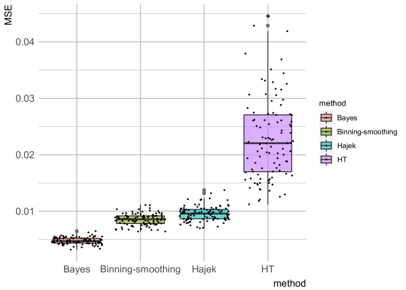
(a) $\theta_{b}\sim\mathcal{U}(0.1,0.9)$

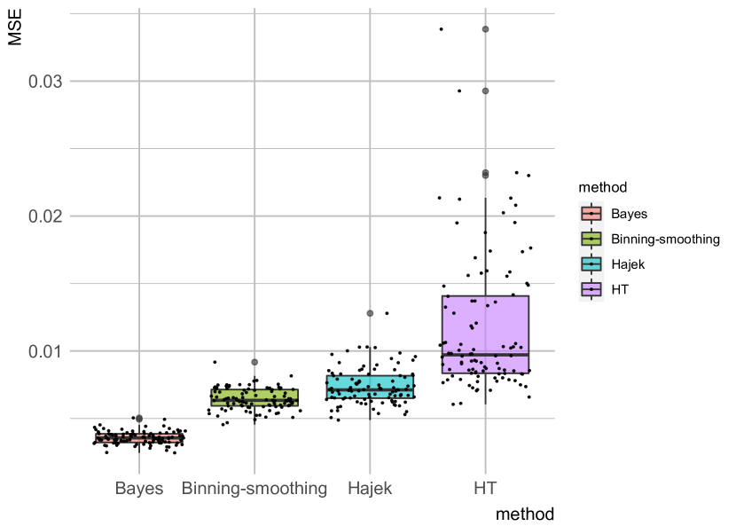
(b) $\theta_{b}\sim\mathcal{U}(0.1,0.4)$

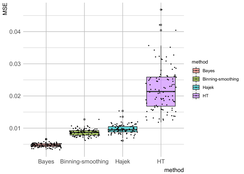
(c) $\theta_{b}\sim\mathcal{U}(0.35,0.65)$

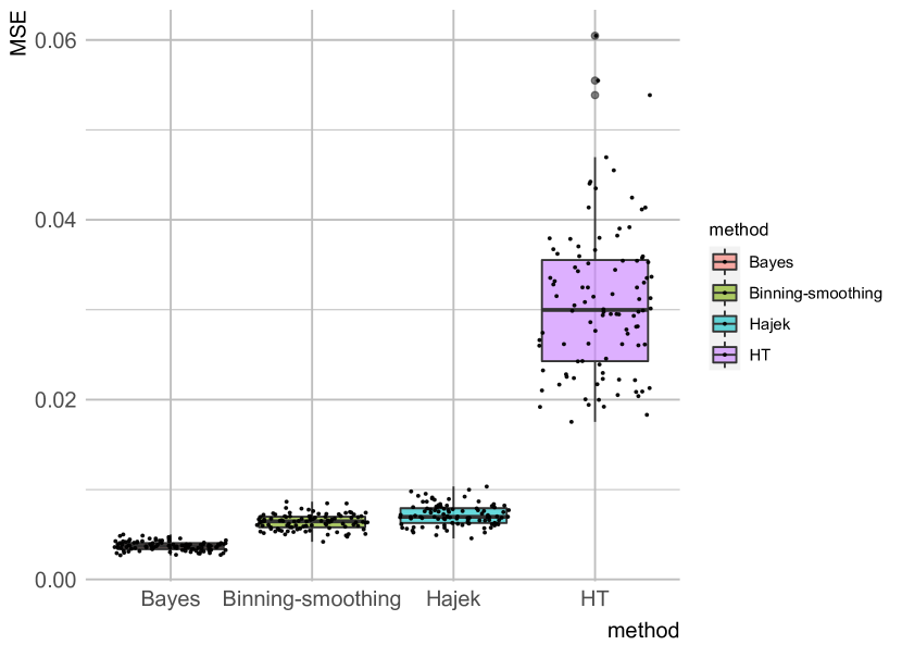
(d) $\theta_{b}\sim\mathcal{U}(0.6,0.49)$

Figure 2: Mean square error comparison for Horvitz-Thompson, Hájek and the Li’s estimator (2.13) for different generative distributions of $\theta_{1},\ldots,\theta_{B}$, and fixed values of $n,B$ and $\delta$. In each case, Bayes’ estimator has the lowest MSE, followed by Hájek, and HT has the largest MSE.

For a single replication with $1,000$ evaluations, Fig. 3 shows the bias and variance for the four candidate estimators. Fig. 3 demonstrates the nature of variance reduction by Bayes’ estimator and the Binning-smoothing idea in estimating $\psi=\mathbb{E}(\boldsymbol{\theta})$ for different ranges of $\theta$, without any significant increase in bias.

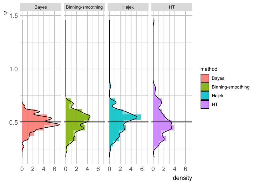
(a) $\theta_{b}\sim\mathcal{U}(0.1,0.9)$

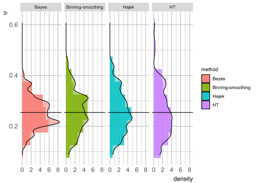
(b) $\theta_{b}\sim\mathcal{U}(0.1,0.4)$

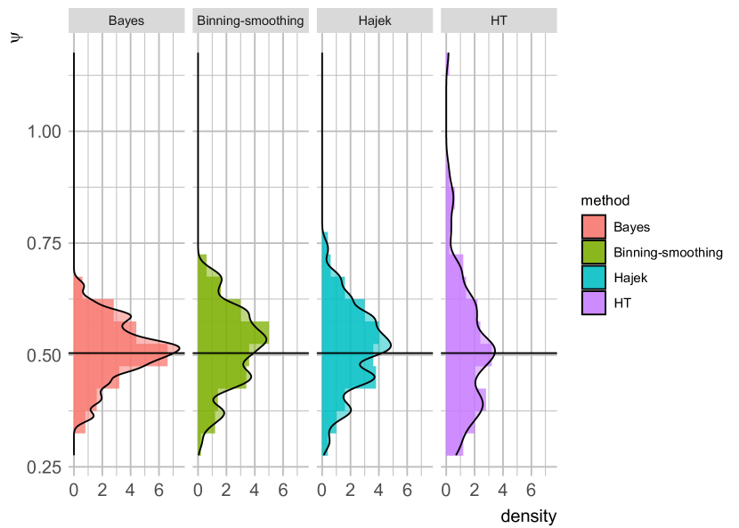
(c) $\theta_{b}\sim\mathcal{U}(0.35,0.65)$

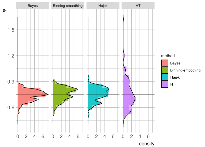
(d) $\theta_{b}\sim\mathcal{U}(0.6,0.49)$

Figure 3: Histogram and Kernel Density plots showing the distribution of Horvitz–Thompson, Hájek and the Bayes estimators for different generative distributions of $\theta_{1},\ldots,\theta_{B}$, and fixed values of $n,B$ and $\delta$.

3.1.2 Missing at random

As discussed earlier, Li’s estimator can be biased when there is a non-zero correlation between $\theta_{X}$ and $p_{X}$, e.g. when the missingness might arise due to confounding. We show an example here to illustrate the effect of this situation, and compare the four candidates. We take $\delta=0.1$, i.e. $p_{b}$’s to be equidistant points in $[0.1,0.9]$, and instead of $\theta_{b}$’s to be uniformly distributed in $[a,b]$, we take:

$$\theta_{b}=\gamma\times p_{b}+(1-\gamma)\times U_{b},\;\text{where}\;U_{b}\sim\mathcal{U}(a,b),\;\gamma=0.5,b=1,\ldots,B.$$

The remaining set-up is same as before. Clearly, in this case the true value of $\psi=\mathbb{E}(\theta)=0.5$. Figure 4(a) shows that the Li’s estimator has an upward bias, as expected, because of the positive correlation between $\theta$ and $p$, but the Hájek and Binned-Smoothed estimators are unaffected. On the other hand, the Binned-Smoothed is significantly better than all the other candidates (HT, Hájek and Li’s) in terms of MSE (Fig. 4(b)). This shows that the Li’s posterior mean estimator can be biased when there is confounding and one needs to be careful when using it. The binned-smoothed method, on the other hand, performs well irrespective of the correlation between $\theta_{X}$ and $p_{X}$, i.e. for both MAR and MCAR-type missingness.

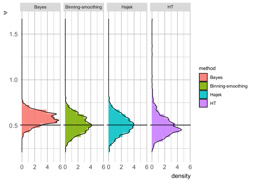
(a) $\theta_{b}=\gamma\times p_{b}+(1-\gamma)\times\mathcal{U}(0,1)$

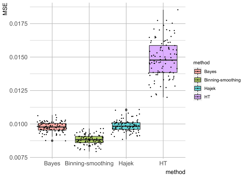
(b) $\theta_{b}=\gamma\times p_{b}+(1-\gamma)\times\mathcal{U}(0,1)$

Figure 4: Histogram, Kernel density plots and MSE comparison for Horvitz–Thompson, Hájek and the Bayes estimators for the missing-at-random scenario.

4 Monte Carlo

A key problem in Bayesian inference is approximating integrals of the form $\psi=\mathbb{E}_{F}\{l(X)\}=\int_{\chi}l({\bf x})dF({\bf x})$ where $l({\bf x})$ is an integrable function of interest and $F(\cdot)$ is finite (e.g. a probability) measure. Integrals of this form are useful for evidence estimation, i.e. approximating $\int_{\Theta}l({\bf y}\mid\boldsymbol{\theta})\pi(\boldsymbol{\theta})d\boldsymbol{\theta}$ where $\theta\in\mathbb{R}^{p}$ is the parameter of interest and $\pi(\boldsymbol{\theta})$ is the prior on $\boldsymbol{\theta}$. Calculating the marginal likelihood is useful for calculating Bayes factor for model selection and other related quantities and also important in statistical mechanics as well as numerical analysis [Liu and Liu, 2001, Robert et al., 1999, Chopin and Robert, 2010]. Evidence estimation or marginal likelihood computation has been one of the most active areas of probabilistic inference spanning a diverse set of applications and we point the interested readers to [Llorente et al., 2020] for a comprehensive review of the advances in evidence estimation. Llorente et al. [2020] categorizes the extant strategies for evidence estimation into four families, viz. methods based on (1) deterministic approximation, (2) density estimation, (3) importance sampling and (4) vertical representation which includes the popular nested sampling [Skilling, 2006]. In this section, we restrict our attention to the third and fourth members in the above taxonomy, viz. importance sampling and vertical likelihood and discuss their connections with the inverse probability weight estimators in survey sampling. Our goal is not to attempt reviewing the huge literature on probabilistic numerical integration or evidence estimation but to emphasize an oft-overlooked point that borrowing ideas from one to the other might lead to improved and more robust estimators for both evidence estimation and survey sampling.

4.1 Importance sampling and vertical likelihood

Given a sample $(y_{1},\ldots,y_{n})$, from either the density $f$ corresponding to $F$ itself or a suitable proposal density $g$, the usual importance sampling estimates $\psi$ by the empirical average:

$$\hat{\psi}_{IS}=\frac{1}{n}\sum_{i=1}^{n}\frac{l(y_{i})f(y_{i})}{g(y_{i})}.$$ (4.1)

If the underlying probability measure is easy to sample from, i.e. if we can afford $f=g$, the above will reduce to the empirical average $\hat{\psi}=n^{-1}\sum_{i=1}^{n}l(y_{i})$, which by the Law of Large Numbers, converge to the true value of $\psi$ at $O(n^{-1})$ rate.

The central idea behind vertical likelihood Monte Carlo [Polson and Scott, 2014, Llorente et al., 2020] is to represent a $p$-dimensional integral $\psi=\int_{\chi}l({\bf x})dF({\bf x})=\int_{\chi}l({\bf x})f({\bf x})d{\bf x}$ as an one-dimensional integral using a latent variable parameter expansion idea. Towards this, first write the integral $\psi$ using the upper cumulant or the survival function of the prior ($f(\boldsymbol{\theta})$) as:

$$\psi=\int_{\chi}l({\bf x})f({\bf x})d{\bf x} =\int_{0}^{\infty}Z(\lambda)d\lambda\;$$

$$\text{where}\;Z(\lambda) =P(\lambda<l({\bf x}))\text{ where }{\bf x}\sim f({\bf x}).$$

Now, consider the inverse function $\Lambda(u)=Z^{-1}(u)=\sup\{\lambda:Z(\lambda)>a\}$. Then it follows from another latent parameter expansion trick that:

$$\int_{0}^{\infty}Z(\lambda)d\lambda =\int_{0}^{1}da\int_{0}^{\infty}\mathbb{I}\{u<Z(\lambda)\}d\lambda$$

$$=\int_{0}^{1}da\int_{0}^{\infty}\mathbb{I}\{\lambda<\Lambda(a)\}d\lambda=\int_{0}^{1}\Psi(a)da.$$ (4.2)

Nested sampling [Skilling, 2006, Chopin and Robert, 2010] uses the identity (4.2) with a quadrature rule: choose a grid of ordered values $a_{n}<a_{n-1}<\ldots<a_{1}<a_{0}\equiv 1$ in $[0,1]$, and use the quadrature formula: $\hat{\psi}=\sum_{i=1}^{m}(a_{i-1}-a_{i})\Lambda(a_{i})$. The deterministic scheme of nested sampling chooses the grid points $a_{i}=\exp(-i/K)$ based on the fact that if $X\sim F$, $Z(L(X))\sim\mathcal{U}(0,1)$ and $Z(\Lambda(a_{i+1}))/Z(\Lambda(a_{i})=a_{i}/a_{i+1}$ follows independent ${\rm Beta}(n,1)$ distribution. This choice of grid points is a judicious one as it chooses the ordinates close to the $\sup l({\bf x})$ region or, in the context of Bayesian evidence, towards higher likelihood $\sup\{l(\theta)\}$ values.

One way to look at this connection between sampling strategies and integral approximation is to represent the former as a missing data problem. Suppose, our goal is to estimate $\psi=\int_{0}^{1}y(x)dx$, which can be thought of as a limiting value of $\psi_{n}=n^{-1}\sum_{i=1}^{n}y_{i}$ as $n\to\infty$, and can be approximated up to any degree of accuracy by $\psi_{N}=N^{-1}\sum_{i=1}^{N}y_{i}$ for a large enough $N$. Given a random sample of size $n\ll N$, with sample probabilities $\pi$ attached to $y_{i}$, we can view estimating $\theta$ as a problem of estimating the population quantity $\psi_{N}$ by $\psi_{n}$. The usual importance sampling estimator in this case is akin to using $\mathbb{E}_{\pi}[\sum_{i=1}^{n}y_{i}/\pi_{i}]=\psi$, the usual HT estimator. Just like the HT estimator, the variance of importance sampling could blow up for poor choices of $g(\cdot)$, while the bias may shrink to zero. As we show below, these connections have been exploited by several authors to propose alternative importance sampling strategies.

The link between evidence estimation and inverse probability weight estimators such as Hájek or Horvitz–Thompson has been studied in literature [see e.g. Barabesi et al., 2003, Barabesi and Marcheselli, 2005, Hesterberg, 1988, 1995, Firth, 2011]. For example, Hesterberg [1988] notes that the weights $f/g$ in (4.1) do not sum to 1, i.e. they are not self-normalized, which is a problem in certain applications, and proposes alternatives based on the sampling strategy such as ratio or regression based weights and a new strategy ‘defensive mixture distributions’. Denoting the weights $W(y)=f(y)/g(y)$, Hesterberg [1988]’s ratio estimator is simply $\hat{\psi}_{\text{ratio}}=\hat{\psi}_{IS}/n^{-1}\sum_{i=1}^{n}f(y_{i})/g(y_{i})$, also known as the self-normalized importance sampling. [Llorente et al., 2020] shows that the infamous harmonic mean estimator [Raftery et al., 2006] as well as the reverse importance sampling scheme [Gelfand and Dey, 1994] are both special cases of self-normalized importance sampling schemes. On the other hand, the regression based estimator using importance weights $f/g$ as potential control variates is given by:

$$\hat{\psi}_{reg}=\sum_{i=1}^{n}V_{reg,i}~{}l(y_{i}),\text{ where, }V_{reg,i}=W_{i}\frac{1+b(W_{i}-\bar{W})}{n},$$

where $b=(1-\bar{W})/\{n^{-1}\sum_{i=1}^{n}(W_{i}-\bar{W})^{2}\}$. Firth [2011] further supports this idea to show that the regression based estimator is asymptotically optimal using the well-known survey sampling fact that the difference estimator $\hat{\psi}_{\gamma}=\hat{\psi}_{IS}+\gamma(1-\bar{W})$ achieves minimum variance with $\gamma=\mathrm{Cov}(\psi f/g,f/g)/\mathbb{V}_{g}(f/g)$.

As discussed in §2, an interesting estimator proposed originally by Trotter and Tukey [1956] as a passing remark and re-discovered by Khan and Ugander [2021] is the adaptive inverse probability weighted (AIPW) estimator. In the context of importance sampling, the estimator will take the form:

$$\hat{\psi}_{AN}=\frac{\sum_{i=1}^{n}l(y_{i})W_{i}}{\lambda n+(1-\lambda)\sum_{i=1}^{n}W_{i}},\;\lambda\in\mathbb{R},\;W_{i}\equiv f(y_{i})/g(y_{i}).$$

Khan and Ugander [2021] shows that the AIPW estimator for the optimal choice of $\lambda$ is algebraically identical to the difference estimators using importance weights as control variates [Owen, 2013, Hesterberg, 1995], although largely ignored in survey sampling and causal inference context [Khan and Ugander, 2021].

4.2 Semiparametric model for Monte Carlo integration

Kong et al. [2003] offer a rigorous theoretical framework for Monte Carlo integration using a semiparametric model where the parameter space is a set of measures on the sample space, possibly infinite-dimensional, and the baseline measure can be approximated by maximum likelihood leading to simple formulae. We reproduce the framework here for sake of clarity and emphasize the connections. As before, consider estimating $\psi(\theta)=\int_{\Gamma}l_{\theta}(x)dF$ where $F$ is a measure on a set $\Gamma$ and $l(\theta)$ is a family of functions $\{l_{\theta}\}$, and the objective is to estimate $\psi(\theta)/\psi(\theta^{\prime})$ for any pair $\theta,\theta^{\prime}$ in this family. The semiparametric model formulation starts with real-valued functions $l_{1},\ldots,l_{k}$ on $\Gamma$ and a non-negative measure $\mu$ on $\Gamma$, with $\psi_{r}\doteq\psi(\theta_{r})$ as before, and the goal is simultaneous estimation of $\psi_{1},\ldots,\psi_{k}$. Now, suppose (simulated) data $(y_{1},x_{1}),\ldots,(y_{n},x_{n})$ are available where $y_{i}\in\{1,\ldots,k\}$ is design-based and $x_{i}\sim P_{y_{i}}$, $i=1,\ldots,n$. Assume that for some $1\leq r\leq k$, $\psi_{r}\in(0,\infty)$ and $n_{r}$ observations are available from $P_{r}(dx)=\psi_{r}^{-1}l_{r}(x)F(dx)$. The likelihood can be written as:

$$\mathcal{L}(F)=\prod_{i=1}^{n}\psi_{y_{i}}^{-1}l_{y_{i}}(x_{i})F(dx_{i}).$$

With the canonical parameter $\theta(x)=\log(F(x))$, we can write the log-likelihood in a fully exponential family form as follows:

$$\ell(F)=\sum_{i=1}^{n}\theta(x_{i})-\sum_{r=1}^{k}n_{r}\log(\psi_{r}(\theta))=n\int_{\Gamma}\theta(x)d\hat{P}_{n}-\sum_{r=1}^{k}n_{r}\log(\psi_{r}(\theta)),$$ (4.3)

where $\hat{P}_{n}$ is the empirical distribution of the values $x_{1},\ldots,x_{n}$, i.e. $\hat{P}_{n}(x)$ $=n^{-1}\sum_{i=1}^{n}\delta_{\{x_{i}\}}(x)$, which can be identified as the canonical sufficient statistics for the canonical parameter $\theta\equiv\theta(x)\in\mathbb{R}^{\Gamma}$. The maximum likelihood estimates follows directly from this exponential family representation and can be written as:

$$\hat{\psi}_{s}=\int_{\Gamma}l_{r}(x)dF=\sum_{i=1}^{n}\frac{l_{r}(x_{i})}{\sum_{r=1}^{k}n_{s}\hat{\psi}_{r}^{-1}l_{r}(x_{i})}$$ (4.4)

where $\hat{\psi}_{r}$ is the MLE of $\psi_{r}$. The algorithm resulting from (4.4) is identified by Kong et al. [2003] as the iterative proportional scaling algorithm of Deming and Stephan [1940] where $n_{r}l_{r}(x_{i})$ is rescaled to $n_{r}l_{r}(x_{i})\hat{F}(x_{i})/\hat{\psi}_{r}$, to form an $n\times k$ array: $\{n_{r}l_{r}(x_{i})\hat{F}(x_{i})/\hat{\psi}_{r}\}_{r=1}^{k}$, with row totals $n_{r}$ and column totals $1$. Kong et al. [2003] points out that the naïve importance sampling (4.1) or the Horvitz–Thompson estimator (2.2) corresponds to the special case $k=1$.

4.3 Quadrature methods

It is worth pointing out that replacing the empirical average for the naïve importance sampling estimator in (4.1) by a Riemann sum estimator provides remarkable improvement in stability and convergence as demonstrated in [Philippe, 1997, Philippe and Robert, 2001] or [Yakowitz et al., 1978]. For example, the Riemann estimator given by:

$$\hat{\psi}_{R}=\sum_{i=1}^{n}(u_{[i+1]}-u_{[i]})l(u_{[i]})f(u_{[i]}),$$ (4.5)

where, $u_{[1]}\leq u_{[2]}\leq\cdots\leq u_{[n]}$ is the order statistics corresponding to points $u_{1},\ldots,u_{n}\in[a,b]$ where $u_{[1]}=a,u_{[n]}=b$. Yakowitz et al. [1978] showed that in the specific case of $a=0,b=1$, taking $u_{1},u_{2},\ldots,u_{n}\sim\mathcal{U}(0,1)$ instead of fixed points in (4.5) will lead to a convergence rate of $O(n^{-4})$ for the variance. Philippe [1997] proved that taking IID samples from any density $f$ will work and lead to the rate $O(n^{-2})$. When the density $f$ is known up to a normalizing constant (say $\tilde{f}$ s.t. $f\propto\tilde{f}$), an alternative form of the Riemann estimator is used with self-normalizing weights [Philippe and Robert, 2001], or a ratio estimator:

$$\tilde{\psi}_{R}=\frac{\sum_{i=1}^{n}(u_{[i+1]}-u_{[i]})l(u_{[i]})\tilde{f}(u_{[i]})}{\sum_{i=1}^{n}(u_{[i+1]}-u_{[i]})\tilde{f}(u_{[i]})}.$$ (4.6)

Philippe and Robert [2001] proposes an extension of the Riemann estimator by replacing $f$ by a Rao–Blackwellized estimate of $f$ provided the conditional densities are analytically tractable.

The quadrature ideas share some commonalities with the binning and smoothing ideas in [Ghosh, 2015] and [Sims, 2010]. These similarities have been utilized in Barabesi et al. [2003], Barabesi and Marcheselli [2005] to construct Riemann estimators for population totals. It is worth noting here that the the environmental studies considered in Barabesi and Marcheselli [2005] fall into a ‘continuous population paradigm’, where sample points are uniformly distributed over a planar region, and continuity of $y(p)$ in $p(\cdot)$ is an underlying assumption for the binned-smoothed estimators. The estimator proposed by Barabesi and Marcheselli [2005] is easily derived from (4.5) by substituting $l(u_{[i]})f(u_{[i]})$ with $y(u_{[i]})$ where $y(u)$ is the intensity of the target variable at location $u$.

4.4 A Bayesian perspective

We conclude the discussion of evidence estimation with a pertinent and profound point raised by Diaconis [1988] in support of Bayesian approaches for probabilistic numerical integration. Diaconis [1988] starts with a algebraic function $f(x)=\exp\{\cosh(\nicefrac{{(x+2x^{2}+\cos x)}}{{(3+\sin x^{3})}}\}$ from $[0,1]\mapsto\mathbb{R}$, for which we want $\int_{0}^{1}f(x)dx$ and asks “What does it mean to ‘know’ a function?.” In such a situation, where we might know a few properties of $f$ and not others, a Bayesian approach seems natural, where one starts with a prior on $\mathcal{C}[0,1]$, the space of continuous functions, and estimate the integral using Bayes’ rule. Diaconis [1988] shows that Brownian motion, the ‘easiest’ prior on $\mathcal{C}[0,1]$, yields a linear interpolation leading to the Trapezoid rule. Diaconis [1988] then shows that a host of well-known methods can be recovered as Bayesian estimates. This key question is revisited in [Owen, 2019] where he asks what does it mean to know the error $\Delta=\lvert\hat{\psi}-\psi\rvert$ and discusses advantages of Bayesian approaches over classical methods. Owen [2019] argues in favour of Bayes methods in difficult problems where extreme cost of function evaluation or skewness or heavy-tailed properties of $l(x)$ or unavailability of central limit theorem exposes the weakness of classical methods.

5 Discussion

Our main goal in this paper was to shed light on various aspects of the family of inverse probability weight estimators, discuss its weakness and strengths and highlight the connections between survey sampling and Monte Carlo integration via these popular tool pervasive in Statistical literature. For survey sampling, we consider some of the ‘weak paradoxes’ [Ghosh, 2015] that arise from using inverse probability estimators using the well-known examples from Wasserman [2004] and Basu [1988], and review the merits and demerits of popular IPW estimators. In particular, we show that the hierarchical Bayes’ estimator due to [Li, 2010] leads to robustness against pathological situations but admits bias in presence of confounding. We provide sufficient conditions for consistency of the Li’s posterior mean estimate in Wasserman’s example and show that, under certain conditions, both the Li’s estimator and the binning-smoothing idea [Ghosh, 2015] achieves lower variation in mean squared errors. We then highlight the analogous tools in Monte Carlo integration, revisiting a few earlier works [e.g. Hesterberg, 1988], where the Horvitz–Thompson estimator is likened to the naïve importance sampling, and much like survey sampling, self-normalized weights or using control variates lead to better estimators. We conclude with a brief discussion of applications in the context of causal inference, a key use of IPW estimators, and a few possible directions for future work.

A possible future direction, borrowing from [Kong et al., 2003] is to use the general semiparametric models and the associated estimators or computational algorithm for $k>1$ in the context of survey sampling that would allow one to combine data from one or more surveys that use different but known inclusion probabilities. We conjecture that this might lead to improved estimators for average treatment effect estimation, which we briefly describe next.

Average Treatment Effect Estimation: A natural application of IPW estimator is average treatment effect (ATE) estimation in potential outcomes causal inference framework as pointed out in [Delevoye and Sävje, 2020, Khan and Ugander, 2021]. We refer the readers to the excellent references in [Cunningham, 2021, Rubin, 1974, Imbens, 2004] for in-depth coverage and historical backgrounds. Here we measure the difference in potential outcomes observed over time points $t_{2}>t_{1}$, where only one of the two potential outcomes are observed for any unit. Using Khan and Ugander [2021]’s notation: we have the triplets $(Y_{k}(0),Y_{k}(1),p_{k})$ for $k=1,\ldots,n$, where we observe $Y_{k}(I_{k})$ for $I_{k}\sim\text{Bernoulli}(p_{k})$. and the parameter of interest is $ATE=\tau=\mathbb{E}[Y_{k}(1)-Y_{k}(0)]$ from the observations available to us. The IPW estimators are employed here to estimate the two population means $\psi_{1}=\mathbb{E}[Y_{k}(1)]$ and $\psi_{0}=\mathbb{E}[Y_{k}(0)]$ separately and estimating $\tau$ by $\hat{\tau}=\hat{\psi_{1}}-\hat{\psi_{0}}$. Estimating the population means $\psi_{j}$, $j=1,2$ turns ATE into a survey sampling problem and one can use all the estimators: HT, Hájek or the various improvements such as the adaptive IPW estimator by Khan and Ugander [2021] based on the Trotter–Tukey idea [Trotter and Tukey, 1956] here. Khan and Ugander [2021] further develop an adaptive estimator by minimizing the variance of between-group differences and show that both the separate AIPW and the joint AIPW estimators achieve lower mean squared errors compared to the usual HT and Hájek.

Thus, a second possible direction for future research is comparing a suitable modification of the Bayes estimator in (2.13) for the ATE problem with that of the adaptive estimators developed by Khan and Ugander [2021] and both empirically and theoretically to investigate consistency properties. It will be also worthwhile to consider the semiparametric model in [Kong et al., 2003] for ATE and compare the results of simultaneous estimation using MLE with these candidates.

Finally, the problems presented in [Wasserman, 2004] and discussed in [Sims, 2010, 2007] are inherently high-dimensional in nature, where sparsity is pervasive. There is a large and growing literature on promoting sparsity in causal inference, e.g. in presence of a large number of confounders or baseline variables while estimating the effect of an exposure on an outcome. We refer the readers to Shortreed and Ertefaie [2017], Wang et al. [2012, 2015], Kim et al. [2022] for recent advances in this area. In our simple focal example, the high-dimensional parameter $\boldsymbol{\theta}=(\theta_{1},\ldots,\theta_{B})$ or ${\bf p}=(p_{1},\ldots,p_{B})$ could exhibit sparsity with a small $\ell_{0}$ norm or other notions of sparsity. To handle sparsity in higher dimensions while maintaining tail-robustness and accuracy, the state-of-the-art Bayesian solution would be augmenting (2.9) with global-local shrinkage priors [Polson and Scott, 2010a, b, 2012, Bhadra et al., 2019], i.e.

$$\theta_{b}\mid\alpha_{T},\psi \stackrel{{\scriptstyle\mathrm{ind}}}{{\sim}}f_{\text{HS}}(\theta;\alpha_{T}\psi,\;\alpha_{T}(1-\psi_{0}),\;\tau)$$

$$f_{\text{HS}}(\theta;a,b,\tau) =\theta^{a-1}(1-\theta)^{b-1}\{1-(1-\theta)\tau^{2}\}^{-(a+b)},$$

$$(\psi,\alpha_{T}\mid\alpha_{F}) \sim\text{Beta}(\alpha_{F},\alpha_{F})\times\pi(\alpha_{T}),$$

$$\;\theta,\psi\in[0,1].$$

Here, as before, $\psi$ is the mean of $\theta$, $\alpha_{T}$ and $\alpha_{F}$ are the and the shape parameters for $\boldsymbol{\theta}$ and $\psi$ respectively and $\tau$ is a global shrinkage parameter adjusting to sparsity. Such Bayesian regularization priors have been used successfully for treatment effect estimation with more control variates than observations [Hahn et al., 2018]. Designing built-in sparsity priors that can also incorporate selection mechanism for confounder selection is an interesting problem that we plan to address in a future endeavor.

Funding

Dr. Datta acknowledges support from the National Science Foundation (DMS-2015460).

References

- Barabesi and Marcheselli [2005] Barabesi, L. and Marcheselli, M. (2005). “Riemann Estimation for Replicated Environmental Sampling Designs.” Journal of Mathematics and Statistics, 1(4): 291–295.
- Barabesi et al. [2003] Barabesi, L. et al. (2003). “A Monte Carlo integration approach to Horvitz-Thompson estimation in replicated environmental designs.” Metron-International Journal of Statistics, 61(3): 355–374.
- Basu [1988] Basu, D. (1988). Statistical information and likelihood: a collection of critical essays by Dr. D. Basu (J. K. Ghosh, Ed.), volume 45. Lecture Notes in Statistics, Springer Science & Business Media.
- Bhadra et al. [2019] Bhadra, A., Datta, J., Polson, N. G., and Willard, B. T. (2019). “Lasso Meets Horseshoe: A Survey.” Statistical Science. Forthcoming.
- Chauvet [2014] Chauvet, G. (2014). “A note on the consistency of the Narain-Horvitz-Thompson estimator.” arXiv preprint arXiv:1412.2887.
- Chopin and Robert [2010] Chopin, N. and Robert, C. P. (2010). “Properties of nested sampling.” Biometrika, 97(3): 741–755.
- Cunningham [2021] Cunningham, S. (2021). “Causal inference.” In Causal Inference. Yale University Press.
- Delevoye and Sävje [2020] Delevoye, A. and Sävje, F. (2020). “Consistency of the Horvitz–Thompson estimator under general sampling and experimental designs.” Journal of Statistical Planning and Inference, 207: 190–197.
- Deming and Stephan [1940] Deming, W. E. and Stephan, F. F. (1940). “On a least squares adjustment of a sampled frequency table when the expected marginal totals are known.” The Annals of Mathematical Statistics, 11(4): 427–444.
- Diaconis [1988] Diaconis, P. (1988). “Bayesian numerical analysis.” Statistical decision theory and related topics IV, 1: 163–175.
- Efron and Morris [1977] Efron, B. and Morris, C. (1977). “Stein’s paradox in statistics.” Scientific American, 236(5): 119–127.
- Firth [2011] Firth, D. (2011). “On improved estimation for importance sampling.” Brazilian Journal of Probability and Statistics, 25(3): 437–443.
- Gelfand and Dey [1994] Gelfand, A. E. and Dey, D. K. (1994). “Bayesian model choice: asymptotics and exact calculations.” Journal of the Royal Statistical Society: Series B (Methodological), 56(3): 501–514.
- Ghosh [2015] Ghosh, J. K. (2015). “Weak Paradoxes and Paradigms.” In Statistical Paradigms: Recent Advances and Reconciliations, 3–12. World Scientific.
- Hahn et al. [2018] Hahn, P. R., Carvalho, C. M., Puelz, D., and He, J. (2018). “Regularization and confounding in linear regression for treatment effect estimation.” Bayesian Analysis, 13(1): 163–182.