Conditional average treatment effect estimation with marginally constrained models

Abstract

Treatment effect estimates are often available from randomized controlled trials as a single average treatment effect for a certain patient population. Estimates of the conditional average treatment effect (CATE) are more useful for individualized treatment decision making, but randomized trials are often too small to estimate the CATE. Examples in medical literature make use of the relative treatment effect (e.g. an odds-ratio) reported by randomized trials to estimate the CATE using large observational datasets. One approach to estimating these CATE models is by using the relative treatment effect as an offset, while estimating the covariate-specific untreated risk. We observe that the odds-ratios reported in randomized controlled trials are not the odds-ratios that are needed in offset models because trials often report the marginal odds-ratio. We introduce a constraint or regularizer to better use marginal odds-ratios from randomized controlled trials and find that under the standard observational causal inference assumptions this approach provides a consistent estimate of the CATE. Next, we show that the offset approach is not valid for CATE estimation in the presence of unobserved confounding. We study if the offset assumption and the marginal constraint lead to better approximations of the CATE relative to the alternative of using the average treatment effect estimate from the randomized trial. We empirically show that when the underlying CATE has sufficient variation, the constraint and offset approaches lead to closer approximations to the CATE.

1 Introduction

Weighing potential benefits and harms of treatment requires knowing the treatment effect, which is the change in probability of an outcome between different treatments. The gold standard for estimating treatment effects are randomized controlled trials (RCTs). RCTs are designed to provide estimates of the average treatment effect (ATE), which reveals if a treatment has an effect on an outcome. The ATE does not reveal which patients would benefit from a treatment. Tailoring the effect to a patient requires knowing how treatment effects change given characteristics of that patient; this is the conditional average treatment effect (CATE). The CATE is a measure of absolute risk, which patients prefer when making decisions [1]. Estimating CATEs directly from RCT data is often infeasible because trials are generally only powered to estimate population average effects.

Under the standard assumptions like ignorability and positivity, observational data provides an avenue for estimating CATEs [2]. However, techniques for observational causal inference often do not make use of knowing the effect provided by an RCT, which are typically reported on a relative scale as an odds-ratio or hazard-ratio (e.g. [3, 4]). To make use of population-level relative effects reported by RCTs in CATE estimation, several previous studies on breast cancer and cardiovascular disease used the assumption of a constant relative treatment effect to develop CATE models from observational data [5, 6, 7, 8]. We call this assumption the constant-relative ATE (CR-ATE) assumption and models that use this assumption CR-ATE models.

The assumption of a constant relative treatment effect does not imply the CATE must be constant because even with a constant relative treatment effect, the treatment can have a varying effect on an absolute risk scale depending on the untreated risk of a patient. For instance, assume that a new cholesterol lowering drug reduces the risk of cardiovascular death within the next 10 years with an odds-ratio of 0.5. A 60-year-old male smoker with hypertension and raised cholesterol has an untreated risk of cardiovascular death of 40% and should expect a reduction in risk of 15% points. A 50-year-old female without hypertension has an untreated risk of under 1% and will have a less than 0.5% points reduction in risk. Given these widely different effects on an absolute probability scale, one may recommend the new cholesterol lowering drug to the 60-year-old male but not the 50-year-old female.

One approach to use the CR-ATE assumption with observational data is to use the constant relative treatment effect as an offset term in a model. Some models built with an offset term were found to be accurate in observational validation studies, on the basis of which treatment guidelines acknowledged a place for them in clinical decision making [9, 10]. Because CR-ATE models target interventional distributions, the use of such model implicitly assumes that the RCT’s relative effect provides the correct offset and that its use controls for unobserved confounding. However, whether the assumption is correct has not been discussed or verified.

In this work we evaluate the validity of the assumption that a known constant odds-ratio for treatment allows for CATE estimation when using the known odds-ratio as an offset term. Under the standard requirements for observational causal inference, we show there is a mismatch in that the odds-ratios reported in RCTs are not the odds-ratios that are needed for the offset method because RCTs generally report estimates of the marginal odds-ratio, whereas the offset method requires the conditional odds-ratio. Further, when there is unobserved confounding, we demonstrate that even with the correct conditional odds-ratio offsets are not sufficient for estimating CATEs.

To address the mismatch in odds-ratios, we introduce a new estimator called the marginally constrained model (MCM). The MCM constrains a model’s implied marginal odds-ratio to be close to that reported from a RCT. We show that with no unobserved confounding this approach is a consistent estimator of the CATE, and we empirically show a large reduction in the number of samples needed to estimate the CATE when using this marginal odds-ratio constraint. We also show how this regularizer can be combined with the CR-ATE assumption in constant-relative marginally constrained model (CR-MCM) models.

Next we turn to violations of ignorability, i.e. the assumption of no unobserved confounding. Without ignorability in offset models, consistent estimation of CATEs is not possible. However, the goal here is to study if models like the CR-MCM approximate the CATE better than the alternative provided by randomized trials, the ATE. The measure of better is the precision in heterogeneous treatment effect estimation (PEHE) [11]. For example, the ATE is a good approximation of the CATE when the underlying CATE has little variation as a function of the conditioning set. Better approximations to the CATE can lead to patient benefit as the CATE leads to better individualized treatment decisions. We empirically show in the absence of ignorability that MCMs almost always lead to better CATE estimation than the average treatment effect-baseline (ATE-baseline) whenever there is sufficient variation in the underlying CATE. Finally, we demonstrate the utility of the CR-ATE assumption and show that when the assumption holds, CR-MCMs are even better than MCMs.

2 Offset models: estimation and non-collapsibility

We consider models for the absolute difference in probability of a binary outcome $Y$ under two possible treatments $T\in\{0,1\}$ conditional on a pre-treatment covariate vector $X$, using data from the observational distribution $q(Y,T,X)$. The estimation target is the CATE, conditional on $X$. Without loss of generality, treatment $T=0$ is assumed to be the baseline treatment (or no treatment depending on the clinical context) and $T=1$ is the comparator treatment of interest. We denote $Y_{t}$ as the potential outcome of $Y$ if $T$ is set to $t$ by intervention, and $Y_{t}|x$ as the analogous potential outcome conditional on $X=x$. We refer to $\Pr(Y_{0}=1|X)$ as the untreated risk, meaning the probability of experiencing the outcome when assigned no treatment (or the control treatment), conditional on $X$. The CATE is defined as:

$$\text{CATE}(x):=\Pr(Y_{1}=1|x)-\Pr(Y_{0}=1|x)$$ (1)

Taking the expected value over $X$ of the CATE, we get the ATE. Working backwards from the definition of the ATE:

ATE $$=\operatorname{\mathbb{E}}[Y_{1}-Y_{0}]$$

$$=\Pr(Y_{1}=1)-\Pr(Y_{0}=1)$$

$$=\operatorname{\mathbb{E}}[\Pr(Y_{1}=1|x)]-\operatorname{\mathbb{E}}[\Pr(Y_{0}=1|x)]$$

$$=\operatorname{\mathbb{E}}\left[\Pr(Y_{1}=1|x)-\Pr(Y_{0}=1|x)\right]$$

$$=\operatorname{\mathbb{E}}\left[\text{CATE}(x)\right]$$ (2)

The ATE (Equation 2) is one measure of treatment effect based on the marginal potential outcomes $Y_{0},Y_{1}$. In addition to the ATE expressed in absolute probabilities, a common measure of treatment effect for binary outcomes employed by RCTs is the marginal odds-ratio (e.g. [3, 4, 12, 13, 14]):

$$\text{OR}(Y_{1},Y_{0})=\frac{\Pr(Y_{1}=1)(1-\Pr(Y_{0}=1))}{(1-\Pr(Y_{1}=1))\Pr(Y_{0}=1)}$$ (3)

It is often more convenient to work with the log odds-ratio. Writing $\sigma(x)=(1+e^{-x})^{-1}$ as the sigmoid function (also known as the logistic function) with its inverse $\sigma^{-1}$ (known as the logit function), the log odds-ratio denoted as $\gamma$ is:

$$\gamma=\gamma(Y_{1},Y_{0})=\log\text{OR}(Y_{1},Y_{0})=\sigma^{-1}(\Pr(Y_{1}=1))-\sigma^{-1}(\Pr(Y_{0}=1))$$ (4)

The log odds-ratio $\gamma$ as a function of potential outcomes $Y_{0},Y_{1}$ is a measure of causal treatment effect. Throughout we will assume to have access to $\gamma$ from a RCT conducted in the same population as the observational study. We assume that this RCT provides an unbiased estimate of the treatment effect measure $\gamma$ with infinite precision. However, as is typically the case due to data-sharing restrictions, only $\gamma$ is available from the RCT and not the original data. Though RCTs can estimate many other parameters of $Y_{t}|X$ such as the conditional odds-ratio [15, 16], in practice they often only report a marginal effect. In the discussion section we describe ways to relax these assumptions.

2.1 Offset models as CATE models

We now study of a class of constant-relative ATE (CR-ATE) models that are already used in clinical practice: offset models [5]. Relying on an assumed functional form of $\Pr(Y_{t}|X)$, offset models aim to approximate $\Pr(Y_{t}|X)$ in a constrained way by forcing the ‘effect’ of treatment to be equal to some known, constant, relative treatment effect on an appropriate scale. In the context of binary outcomes, one CR-ATE assumption is that the odds-ratio for treatment is constant for all $X$, whereas the untreated risk $\Pr(Y_{0}=1|X)$ varies with $X$, meaning that:

$$\Pr(Y_{t}=1|x)=\sigma\left(\sigma^{-1}(\Pr(Y_{0}=1|x))+\beta_{t}t\right).$$ (5)

The assumption in Equation 5 is called the offset assumption for logistic models and is an example of a constant-relative treatment effect assumption. Note that $\beta_{t}$ is a measure of treatment effect derived from the conditional potential outcomes $Y_{0}|X,Y_{1}|X$, and the specific offset assumption is that $\beta_{t}$ does not depend on $X$. Using this assumption with also assuming $\beta_{t}$ is known yields a class of models of $\Pr(Y_{t}=1|X)$ called $g:\{0,1\}\bigtimes\mathcal{X}\to[0,1]$, defined as:

$$g(t,x)=\sigma\left(\sigma^{-1}(g_{0}(x))+\beta_{t}t\right),$$ (6)

where $g_{0}=g(0,x):\mathcal{X}\to[0,1]$. In the context of generalized linear models, a fixed term in a model that is not estimated from data is called an offset term [17]. We therefore refer to models of the form of Equation 6 as treatment offset models or offset models for short. Later we will study under what conditions offset models lead to consistent estimators of the CATE.

Offset models and analogous CR-ATE models have been used in practice without any justification [5, 6, 7, 8]. Though the parametric assumption in Equation 5 may seem strong, one supporting argument is that the odds-ratio was a more stable measure of treatment effect than the absolute risk difference in a review of 125 meta-analyses of RCTs [18]. Additionally, RCTs rarely find evidence for variation in the odds-ratio depending on covariates (i.e. interaction terms between covariates and treatment on the log-odds scale), though it should be noted that RCTs are generally underpowered for estimating these interaction terms. Either way, the fact that offset models are used in practice warrants a formal understanding of their consistency and under what conditions they are likely to provide a better approximation to the CATE than the ATE-baseline.

2.2 Estimation of offset models

To study offset models we must first describe how they may be estimated. One can construct an estimator for offset models of the form in Equation 6 by specifying a class of functions $\mathcal{G}_{0}=\left\{g_{0}\in\mathcal{G}_{0}:\mathcal{X}\to[0,1]\right\}$ for the untreated risk $\Pr(Y_{0}=1|X)$. Assume that $X$ is discrete with cardinality $d$. Coding $X$ as a $d$-dimensional one-hot vector leads to a natural parameterization for non-parametric models of $\Pr(Y_{0}=1|X)$ with $d$ logistic regression parameters $\bm{b}\in\mathbb{R}^{d}$, giving rise to model family $\mathcal{G}_{0}=\{g_{0}:\mathcal{X}\to[0,1],g_{0}(x;\bm{b})=\sigma(\bm{b}^{\prime}x),\bm{b}\in\mathbb{R}^{d}\}$. This $\mathcal{G}_{0}$ together with a known $\beta_{t}$ defines a family of offset models:

$$\mathcal{G}=\left\{g:\{0,1\}\bigtimes\mathcal{X}\to[0,1],g(t,x;\bm{b},\beta_{t})=\sigma\left(\bm{b}^{\prime}x+\beta_{t}t\right),\bm{b}\in\mathbb{R}^{d}\right\}$$ (7)

Parameter vector $\bm{b}$ may be obtained by maximizing the likelihood of the observed data. The question is under what conditions this yields a consistent estimator of $\Pr(Y_{t}=1|X)$. If for every $x\in\mathcal{X},0<\Pr(Y_{0}=1|X=x)<1$, there is always a $\bm{b}^{*}\in\mathbb{R}^{d}$ such that $\Pr(Y_{0}=1|x)=\sigma(\bm{b}^{*\prime}x)$. With this $\bm{b}^{*}$ we have that by the offset assumption:

$$g^{*}(t,x;\bm{b}^{*}) :=\sigma\left(\bm{b}^{*\prime}x+\beta_{t}t\right)$$

$$=\sigma\left(\sigma^{-1}(\Pr(Y_{0}=1|x))+\beta_{t}t\right)$$

$$=\Pr(Y_{t}=1|x)$$

Collapsibility.

An important concept when considering offset models is collapsibility. A measure $\mu(Y_{0},Y_{1})$ of causal effect is said to be collapsible over variable $X$ if there exist a set of weights $w_{x}$ such that $\mu(Y_{0},Y_{1})=\frac{1}{\sum w_{x}}\sum w_{x}\mu(Y_{0},Y_{1}|x)$, meaning that the marginal effect is a weighted average of the $x$-conditional effects [19, 20]. As shown in Equation 2 the ATE is a collapsible effect measure by weighting the CATEs by the probability of $X$. For odds-ratios, except for very special circumstances, there are no such weights meaning that the odds-ratio is non-collapsible [21, 22].

The non-collapsibility of the odds-ratio creates a problem for estimating logistic offset models as the marginal log odds-ratio $\gamma$ reported in the RCTs is not equal to the conditional log odds-ratio $\beta_{t}$ required in Equation 6. This means that the model in Equation 6 cannot be estimated from the available data. The stronger the $T$-conditional association between $X$ and $Y$, the greater the difference between $\gamma$ and $\beta_{t}$ [23]. For an illustration, see Appendix A.1. This mismatch is an important drawback as at the same time, a stronger association between $X$ and $Y$ conditional on $T$ results in more variation in $\Pr(Y_{0}|X)$ and thus more variation in the CATE under the constant-relative treatment effect assumption. So in the situation where offset models have more potential added value (when the CATEs vary substantially), the estimate of the marginal log odds-ratio $\gamma$ from RCTs becomes a less accurate approximation of the conditional odds-ratio $\beta_{t}$ needed for estimating the offset model. If one were to use $\gamma$ in the place of $\beta_{t}$ in Equation 6, this would lead to an inconsistent estimator. We provide a numerical example in the experiments section (Section 5.2) that highlights this effect of non-collapsibility on offset models.

3 Marginally Constrained Models

We now turn to a new class of CATE models that also exploits knowledge from prior RCTs. There are many instances where an estimate of $\gamma$ is available from the published results of an RCT, but not the CATE because the sample size of the RCT was too small. Running a new, bigger RCT may be infeasible due to costs, or deemed unethical because of the absence of equipoise, i.e. uncertainty about what treatment is superior if the prior RCT demonstrated that one treatment was superior over the other on average. When turning to observational data to estimate the CATEs, instead of ignoring the $\gamma$ estimate from the RCT, we can use it in the estimation as a constraint. We describe a procedure for incorporating $\gamma$ in CATE estimation based on the marginalization of predicted outcome probabilities. Under some regularity conditions, we prove that this method leads to a consistent estimator of the CATE when the standard causal inference assumptions hold.

3.1 Exploiting RCT evidence by using the marginal odds-ratio as a constraint

Assume we have a function $g$ from a family of functions $\mathcal{G}=\left\{g:\{0,1\}\bigtimes\mathcal{X}\to[0,1]\right\}$ where we interpret $g(t,x)$ as a predicted probability $\Pr(Y=1|t,x)=g(t,x)$. Given a distribution $q$ over $X$, we can calculate the marginalized predictions of $g$: $\Pr(Y=1|t)=\operatorname{\mathbb{E}}_{x\sim q(x)}g(t,x)$. Correspondingly we have the implied marginal log odds-ratio $M(g)$ (implied by $g$ and $q$, but suppressing the dependency on $q$ in the notation) by using the marginalized predictions of $g$ over $q$.

$$M(g)=\sigma^{-1}(\operatorname{\mathbb{E}}g(1,X))-\sigma^{-1}(\operatorname{\mathbb{E}}g(0,X))$$ (8)

Given an independent and identically distributed sample of $X$ with sample size $n$, define the empirical counterpart of $M$ as:

$$M_{n}(g)=\sigma^{-1}(\frac{1}{n}\sum_{i=1}^{n}g(1,x_{i}))-\sigma^{-1}(\frac{1}{n}\sum_{i=1}^{n}g(0,x_{i}))$$ (9)

This empirical marginalizer was used in [22]. Assume $g$ was found by maximizing the log-likelihood of the observed data over function class $\mathcal{G}$, $L_{n}:\mathcal{G}\to\mathbb{R}$. We can augment the optimization objective using the known marginal odds-ratio $\gamma$ from the prior RCT as follows:

$$\mathcal{L}_{n}(g)=L_{n}(g)-\lambda(M_{n}(g)-\gamma)^{2},\lambda>0$$ (10)

We call optimization with the objective a marginally constrained model (MCM). If $\mathcal{G}$ encompasses all conditional distributions on $\{0,1\}\bigtimes\mathcal{X}$, i.e. in the non-parametric estimation setting, it follows that $\exists g*\in\mathcal{G}$ such that $g^{*}(t,x)=\Pr(Y_{t}=1|x)$. Assume that additionally the standard observational causal inference assumptions hold, namely: $(Y_{1},Y_{0})\perp\!\!\!\perp T|X$ (strong ignorability), $0<q(T|X)<1$ (positivity) and $Y_{t}=Y$ if $T=t$ (consistency). For more details on these assumptions see e.g. [24, 25]. Theorem 1 states that under these conditions, the augmented objective 10 yields a consistent estimator of $\Pr(Y_{t}=1|X)$.

Theorem (informal) 1.

Given binary treatment $T$, binary outcome $Y$ and covariate $X$. Assume strong ignorability $(Y_{1},Y_{0})\perp\!\!\!\perp T|X$, positivity $0<q(T|X)<1$ and consistency $Y_{t}=Y$ if $T=t$. Given a family of functions $\mathcal{G}=\left\{g\in\mathcal{G}:\{0,1\}\bigtimes\mathcal{X}\to[0,1]\right\}$ and assuming $\exists g^{*}\in\mathcal{G},\Pr(Y_{t}=1|x)=g^{*}(t,x)$. Denote the sample log-likelihood $L_{n}:\mathcal{G}\to\mathbb{R}$. In addition, given marginal log odds-ratio $\gamma=\sigma^{-1}(\Pr(Y_{1}=1))-\sigma^{-1}(\Pr(Y_{0}=1))$, sample marginalizer $M_{n}:\mathcal{G}\to\mathbb{R}$ and $\lambda>0$. Then:

$g_{n}=\arg\max_{g\in\mathcal{G}}\left[L_{n}(g)-\lambda(M_{n}(g)-\gamma)^{2}\right]$ is a consistent estimator of $\Pr(Y_{t}=1|X)$

For proving consistency, additional assumptions on convergence and identifiability of the observational objective are required. The formal theorem statement and proof are provided in the Appendix A.2. Under the conditions of Theorem 1, both the unconstrained maximum-likelihood estimator and the marginally constrained estimator are consistent estimators of the CATE. However, as the MCM optimizes over a smaller family of functions, we should expect it to be more statistically efficient. We test the relative efficiency of the MCM versus the unconstrained estimator in the experiments section 5.1.

3.2 Marginally constrained constant-relative treatment effect model estimation

MCM leverages knowledge of the marginal odds-ratio $\gamma$ for CATE estimation but it does not use the offset-assumption from Equation 5. Offset models do rely on this assumption but often cannot be estimated because the required conditional odds-ratio is not known. We now introduce the constant-relative marginally constrained model (CR-MCM), a CATE model that leverages both the offset assumption and a known marginal odds-ratio $\gamma$. With discrete $X$ of cardinality $d$, non-parametric modeling of $\Pr(Y_{t}|X)$ requires $2d$ parameters, $d$ parameters for $\Pr(Y_{0}|X)$ and $d$ additional parameters for $\Pr(Y_{1}|X)$. The offset assumption in Equation 5 implies that there exists a $\bm{b}^{*}\in\mathbb{R}^{d}$ and $\beta_{t}$ such that $\sigma\left(\bm{b}^{*\prime}x+\beta_{t}t\right)=\Pr(Y_{t}=1|x)$. To exploit the offset assumption in MCMs and reduce the number of parameters, we can use the constrained objective in Equation 10 and consider optimizing over the offset model family in Equation 7. However, without access to $\beta_{t}$, the model family is underspecified and we cannot proceed with optimization. Instead we introduce CR-MCM as:

$$\bm{b},b_{t}=\arg\max_{\bm{b}\in\mathbb{R}^{d},b_{t}\in\mathbb{R}}\left[L_{n}\left(g(t,x;\bm{b},b_{t})\right)-\lambda\left(M_{n}\left(g(t,x;\bm{b},b_{t})\right)-\gamma\right)^{2}\right],\lambda>0$$ (11)

The model family for CR-MCM has $d+1$ parameters and by the offset assumption $\exists\bm{b}^{*},b_{t}^{*}\in\mathbb{R}^{d}\bigtimes\mathbb{R}$, $g(t,x;\bm{b}^{*},b_{t}^{*})=\Pr(Y_{t}=1|x)$. Because this model family is a correctly specified generalized linear model, maximizing the (unconstrained) likelihood over this family is a consistent estimator of $\Pr(Y=1|T,X)$. Given strong ignorability, positivity and consistency, $\Pr(Y=1|T,X)=\Pr(Y_{t}=1|X)$. Under the regularity conditions of Theorem 1 we have that Equation 11 is a also consistent estimator of $\Pr(Y|T,X)$. Moreover, CR-MCM may be more efficient than MCM when the offset assumption holds.

4 Offset models and marginally constrained models for CATE approximation under unobserved confounding

We now turn to the case where the standard assumption of strong ignorability does not hold: in the presence of unobserved confounding. In the presence of unobserved confounding, meaning that $Y_{t}$ is not independent of $T$ conditional on $X$, CATE estimators based on adjustment cannot be used. However, this does not preclude causal effect estimation as there are known settings where causal effects can be determined despite the presence of unobserved confounding if one can rely on additional assumptions regarding the data generating mechanism. Example methods are instrumental variable estimation [26, 27, 28] and methods based on proxy-variables of unmeasured confounders [29, 30].

4.1 Offset models under unobserved confounding

We investigate whether the structural assumption made in the offset model in Equation 5 combined with knowledge of the conditional odds-ratio $\beta_{t}$ makes the offset model a consistent estimator of the CATE. With a simple counter example, we prove that this is not the case.

Example 1: Offset models are inconsistent estimators in the presence of unobserved confounding

A simple example compatible with the offset assumption in Equation 5 is when there is a binary unobserved confounder $U$ but no covariate $X$. Denoting $\mathcal{B}$ as the Bernoulli distribution and $q_{u}=\Pr(U=1)$, then the data-generating mechanism for this example is:

$$u\sim\mathcal{B}(q_{u}),t\sim\mathcal{B}(\Pr(T=1|u)),y\sim\mathcal{B}(\Pr(Y_{t}=1|u))$$ (12)

Given the offset model family from Equation 7, a natural parameterization of $g(t,x)=g(t)$ in the context of this example is $g(t;b_{0})=\sigma(b_{0}+\beta_{t}t),b_{0}\in\mathbb{R}$. To disentangle the issue of non-collapsibility from unobserved confounding, we assume that $\beta_{t}$ is given a-priori and is not estimated. We derive a closed-form expression for the expected log-likelihood of the observational data depending on the single parameter $b_{0}$ of the offset model $L(b_{0})$ in the Appendix A.3. Taking the derivative with respect to $b_{0}$ and plugging in the ground truth value $\beta_{0}:=\sigma^{-1}(\Pr(Y_{0}=1))$ we find the following expression:

$$\frac{\partial L}{\partial b_{0}}\bigl{(}b_{0}=\beta_{0}\bigr{)}=q_{u}(1-q_{u})\bigl{[} (\Pr(Y|T=0,U=1)-\Pr(Y|T=0,U=0))\left(q(T=0|U=1)-q(T=0|U=0)\right)+$$

$$(\Pr(Y|T=1,U=1)-\Pr(Y|T=1,U=0))\left(q(T=1|U=1)-q(T=1|U=0)\right)\bigr{]}$$

In general this expression is non-zero, meaning that the ground truth solution $\beta_{0}$ is not a stationary point of the expected log-likelihood. Thereby the offset method is an inconsistent estimator for $\Pr(Y_{0}=1)$ in the presence of unobserved confounding. When either $q(T|U=1)=q(T|U=0)$ or $\Pr(Y_{t}=1|U=1)=\Pr(Y_{t}=1|U=0)$, the derivative is zero at $\beta_{0}$, meaning that $\beta_{0}$ is a stationary point of the expected log-likelihood. Either of these cases imply no unobserved confounding.

Despite its simplicity this example is important for all offset models with discrete $X$ as a) when the treatment is binary, any arbitrary unobserved confounder can be modeled as a single binary variable while maintaining the same observational and interventional distributions [31]; and b) given $X$ with cardinality $d>1$, optimizing over the offset model family in Equation 7 is equivalent to stratifying the population for each value of $X$ and optimizing the same objective as in Example 1 in each stratum. Thus if the offset model is an inconsistent approximator of $\Pr(Y_{0}=1)$ in this simple example with no covariate $X$, optimization over the offset model family for discrete $X$ will also be inconsistent for $\Pr(Y_{0}|X)$ by implication, even when the correct conditional log odds-ratio $\beta_{t}$ is known. In the Appendix A.3 we show that this implies that the offset model is inconsistent for the CATE as well, aside from very rare chance occasions.

4.2 Metric and average treatment effect baseline

Offset models are not consistent estimators of the CATE in the presence of unobserved confounding and require knowledge of the conditional odds-ratio which is generally not available. However, offset models may still be useful for treatment decisions if they lead to better CATE approximation than what is used in current clinical practice. As RCTs generally only estimate a single average treatment effect (ATE), this is often what current treatment decisions are based on. Ideally, treatment decisions are based on the difference in probability of the outcome under different treatments conditional on patient characteristics, i.e. the CATE. A direct measure for how well a model approximates the CATE is the root-mean-squared error of approximated versus actual CATE. In the context of CATE approximation this metric is sometimes called the precision in heterogeneous treatment effect estimation (PEHE, [11]). The PEHE for function $g:\{0,1\}\bigtimes\mathcal{X}\to[0,1]$ is defined as:

$$\text{PEHE}(g)=\sqrt{\operatorname{\mathbb{E}}\left(\text{CATE}(x)-(g(1,x)-g(0,x))\right)^{2}}$$ (13)

As RCTs only provide the ATE, in our experiments, we use the PEHE of the ATE as the baseline. If the CATE is not constant but varies with $X$, the ATE is a bad approximator of the CATE, leading to suboptimal PEHE and thus suboptimal treatment decisions. Measuring the approximation error with the PEHE is how we arrive at what we call the ATE-baseline: the PEHE that is obtained in the current situation by using a single treatment effect for treatment decisions in all patients, instead of using the CATE. The PEHE of the ATE-baseline is calculated as:

$$\text{PEHE}(\text{ATE})=\sqrt{\operatorname{\mathbb{E}}\left[\left(\text{CATE}(x)-\text{ATE}\right)^{2}\right]}$$ (14)

Given that $\text{ATE}=\operatorname{\mathbb{E}}[\text{CATE}(x)]$, the ATE-baseline has an intuitive form:

$$\text{PEHE}(\text{ATE}) =\sqrt{\operatorname{\mathbb{E}}\left[\left(\text{CATE}(x)-\text{ATE}\right)^{2}\right]}$$

$$=\sqrt{\operatorname{\mathbb{E}}\left[\left(\text{CATE}(x)-\operatorname{\mathbb{E}}[\text{CATE}(x)]\right)^{2}\right]}$$

$$=\sqrt{\text{VAR(CATE)}}$$

$$=\text{SD(CATE)}$$ (15)

For CATE approximation models such as the offset model and the MCM and CR-MCM, even if the model is inconsistent under certain conditions, it may still be a valid modeling choice if it has lower PEHE than the ATE-baseline because it can lead to better treatment decisions compared with current clinical practice.

5 Experiments

We now study the different models for CATE approximation in four experiments. In the Appendix (A.4), we derive a closed-form solution for the parameters of the offset model in the case of a binary covariate. This closed-form can be used to characterize the bias in offset solutions, though the resulting formula is opaque. Therefore, we use the closed form for an extensive empirical evaluation. First we investigate the relative efficiency of the MCM compared to unconstrained estimation when both are consistent. Then we investigate the PEHE of the offset model under a) non-collapsibility but no unobserved confounding and b) unobserved confounding but no non-collapsibility. Finally, we compare the PEHE of three different CATE approximators: the offset model with marginal odds-ratio $\gamma$, MCM and CR-MCM and study when these models have better PEHE than the ATE-baseline in a large experimental grid with a binary covariate and an unobserved confounder $U$.

Implementation.

For implementing MCM and CR-MCM, we optimize the constrained objective 10 by specifying a small value $\lambda_{0}=0.01$ and optimizing the resulting unconstrained objective with a LBFGS optimizer. After convergence of the unconstrained optimizer yielding model estimate $\hat{g}$, we evaluate the constraint $(M(\hat{g})-\gamma)^{2}<\epsilon=10^{-4}$. If this is not satisfied, for the next iteration $i=1,2,...$ we increase $\lambda$ such that $\lambda_{i}=10*\lambda_{i-1}$ and repeat until the constraint is satisfied. We relied on the JAX [32], JAXOpt [33] and NumPyro [34] python libraries for implementing the experiments. The code to reproduce all experiments is publicly available at www.github.com/vanamsterdam/binarymcm (DOI: 10.5281/zenodo.8144896).

5.1 Relative efficiency of the marginally constrained estimator

Under the assumptions of strong ignorability, positivity and consistency and with a known marginal odds-ratio $\gamma$, we have at least two consistent estimators of the CATE: the unconstrained maximum-likelihood estimator and the marginally constrained model (MCM). In order to test the relative efficiency of the constrained versus the unconstrained estimator, we define an experimental grid with a binary covariate $X$ and data generating mechanism $\sigma^{-1}(\Pr(Y_{t}=1|x))=\beta_{0}+\beta_{t}t+\beta_{x}x$. The parameter grid is given in Table 1.

Table 1: Grid for experiment on relative efficiency of the marginally constrained versus the unconstrained estimator

parameter	definition	values
$q_{x}$	$\Pr(X=1)$	0.5
$\beta_{0}$	$\sigma^{-1}(\Pr(Y_{0}=1|X=0))$	$\sigma^{-1}(0.15,0.5)$
$\beta_{t}$	$\sigma^{-1}(\Pr(Y_{1}=1|X))-\sigma^{-1}(\Pr(Y_{0}=1|X))$	1
$\beta_{x}$	$\sigma^{-1}(\Pr(Y_{t}=1|X=1))-\sigma^{-1}(\Pr(Y_{t}=1|X=0))$	log(1/5, 1/2, 1, 2, 5)
$q_{t}$	$\Pr(T=1)$	0.5
$\eta_{x}$	$\sigma^{-1}(\Pr(T=1|X=1))-\sigma^{-1}(\Pr(T=1|X=0))$	log(1/5, 1/2, 1, 2, 5)
$n$	sample size	50, 75, 100, 150, 200, 325, 400, 500, 750

In this setup, a non-parametric model family for $\Pr(Y_{t}=1|X)$ is

$$\mathcal{G}=\left\{g:\{0,1\}^{2}\to[0,1],g(t,x)=\sigma(b_{0}+b_{t}t+b_{x}x+b_{tx}tx),b_{0},b_{t},b_{x},b_{tx}\in\mathbb{R}\right\}$$

Given this model family, sample log-likelihood estimator $L_{n}$, sample marginalizer $M_{n}$, and marginal log odds-ratio $\gamma$ (calculated from the parameters of the data generating mechanism), we compare the constrained and unconstrained estimator. For each of the possible combinations of parameter values in Table 1, we generated 250 datasets and applied both estimators. Each fitted model produces an estimate of CATE $(X=0)$ and CATE $(X=1)$. We construct 95% confidence bounds for these estimated CATEs by taking the 2.5% and 97.5% percentile-values over the 250 repetitions for each simulation setting, sample size, estimator and $X$. The width of each confidence bound (len(CI)) is a measure of statistical uncertainty that is relevant for treatment decision making. As expected by asymptotic theory for asymptotically linear normal estimators, we found empirically that $\log(\text{len(CI)})$ was approximately linear in the logarithm of the sample size for each parameter setting and estimator, see Figures 4, 5 in the Appendix. We fit models to the experimental results to summarize the relative efficiency. Specifically, denoting $m=1$ to indicate the unconstrained estimator and $m=0$ for the constrained estimator, we fit linear regression models of the form $\log n=w_{0}+w_{l}\log(\text{len(CI)})+w_{m}m+\epsilon$ to the experimental results of each parameter combination. We took len(CI) to be the average of the logarithm of the confidence bound length of CATE $(X=1)$ and CATE $(X=0)$ in each experiment.

The linear models provided a good fit of the experimental results with an adjusted $R^{2}>0.975$ for all of the combinations of simulation parameters. The parameter $w_{m}$ in this linear model has the following interpretation: if sample size $n_{c}$ reaches a certain length of the confidence bound with the constrained estimator, to reach the same length of the confidence bound with the unconstrained method, $n_{c}e^{w_{m}}$ samples are needed, meaning a $100(e^{w_{m}}-1)$% increase in sample size. Across all simulation settings, we find that unconstrained estimation requires at least 71% and at most 106% more samples, meaning that to achieve equal-width confidence bounds in the CATE estimation one needs at least 71% more patients with the unconstrained estimator then when using the constrained estimator MCM.

5.2 The effect of non-collapsibility on the offset method

When the offset method is applied using the marginal log odds-ratio $\gamma$ in the place of conditional log odds-ratio $\beta_{t}$, the offset model is inconsistent and has non-zero PEHE. We conducted a numerical experiment to evaluate the PEHE of the offset model compared with the ATE-baseline and CR-MCM with a single binary covariate $X$ with varying effect on $Y$. The data-generating mechanism for this experiment is $\sigma^{-1}(\Pr(Y_{t}=1|x))=\beta_{0}+\beta_{t}t+\beta_{x}x$, with $\beta_{0}=0,\beta_{t}=1,0\leq\beta_{x}\leq\log 15=2.71$. Furthermore, $\Pr(X=1)=\Pr(T=1)=0.5$.

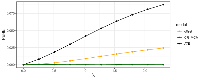
Figure 1: Experiment on the effect of non-collapsibility on the offset model when the marginal log odds-ratio $\gamma$ is used instead of the conditional log odds-ratio $\beta_{t}$, for varying effects of $X$ on $Y$. When the outcome depends more on covariate $x$ (i.e. bigger $\beta_{x}$) the difference between the marginal odds-ratio and conditional odds-ratio becomes bigger due to non-collapsibility of the odds-ratio, leading to worse CATE approximation error for the offset model. The CR-MCM model uses the marginal odds-ratio as a constraint and remains consistent. CR-MCM: constant-relative marginally constrained model, ATE: average treatment effect

In Figure 1 we see that when $\beta_{x}$ increases, the PEHE of the offset model with $\gamma$ as an offset increases as expected due to the increasing difference between $\gamma$ and $\beta_{t}$. However, the PEHE of the ATE-baseline increases faster. Finally, we note that the CR-MCM remains consistent as by Theorem 1.

5.3 The effect of unobserved confounding on the offset method

When the strong ignorability does not hold, for example due to the presence of an unobserved confounder $U$, Example 1 (section 4.1) demonstrates that the offset model is an inconsistent estimator of $\Pr(Y_{t}=1)$, even if the conditional log odds-ratio $\beta_{t}$ is known. As motivated before, it may still be justifiable to use the offset method when it has better PEHE than the ATE-baseline. To study the effect of unobserved confounding on the PEHE of the offset method, we conducted an experiment with a binary covariate $X$, binary unobserved confounder $U$ and in this case a known conditional log odds-ratio $\beta_{t}$. We note that this $\beta_{t}$ is generally not available from RCTs, but we use it in this experiment to separate out the effect of unobserved confounding from non-collapsibility. The data-generating mechanism for this experiment is:

• $\sigma^{-1}(\Pr(Y_{t}=1|X=x,U=u))=\alpha_{0}+\alpha_{t}t+\alpha_{x}x+\alpha_{tx}tx+\alpha_{u}u$

• $\Pr(U|T=t)$ such that $\sigma^{-1}(\Pr(U=1|T=1))-\sigma^{-1}(\Pr(U=1|T=0))=\gamma_{u}=\alpha_{u}$.

The parameter ranges were $\alpha_{0}=\sigma^{-1}(0.05),\alpha_{t}=1,\alpha_{x}\in\log(1,2,3,4,5),\alpha_{u}\in\log(1,2,5)$. We set the marginals $\Pr(U=1)=\Pr(X=1)=\Pr(T=1)=0.5$. Parameter $\alpha_{x}$ controls the effect of $X$ on $Y$ and $\alpha_{u}$ determines the amount of unobserved confounding (both through $U\to Y$ and $U\to T$). Note that if the offset assumption in Equation 5 is used, it is assumed to hold conditional on the observed covariate $X$, i.e. for distribution $\Pr(Y_{t}|X)$, not for $\Pr(Y_{t}|X,U)$. Therefore, given values for $\alpha_{0},\alpha_{t},\alpha_{x},\alpha_{u},\Pr(U|T=t)$, the parameter $\alpha_{tx}$ was determined such that the offset assumption was valid for $\Pr(Y_{t}|X)$. To implement CR-MCM the marginal log odds-ratio for treatment $\gamma$ was calculated from the experiment parameters.

On this experimental grid four different models are compared: the ATE-baseline, the offset method with conditional odds-ratio, CR-MCM and a ‘fully-observational’ estimator, i.e. the non-parametric maximum likelihood estimator of $q(Y=1|T,X)$ where $q$ denotes the observational distribution. The results are presented in Figure 2. As expected, the PEHE of the fully-observational estimator is very sensitive to increasing amounts of unobserved confounding. The PEHE of the ATE-baseline increases when the variance of the CATE increases, which in this experiment is determined by $\alpha_{x}$. While the PEHE for the offset method increases when unobserved confounding increases, it still has better PEHE than the ATE-baseline when $\alpha_{x}\neq 0$. Finally, CR-MCM is the best performing model overall even though, in contrast with the offset model, does not require knowledge of the conditional odds-ratio $\beta_{t}$ which is generally not available from RCTs.

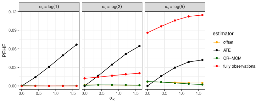
Figure 2: Experiment on the effect of unobserved confounding on the offset estimator when the conditional log odds-ratio $\beta_{t}$ is known but there is an unobserved confounder, for varying effects of $X$ on $Y$. $\alpha_{x}$ determines the effect of $X$ on the outcome $Y$, $\alpha_{u}$ determines the amount of unobserved confounding. When $\alpha_{x}$ gets bigger, the average treatment effect becomes a bad approximator for the CATE. When unobserved confounding increases, the fully observational baseline becomes a bad approximator of the CATE as expected. Both the offset model and the CR-MCM perform well, although the offset model requires knowledge of the conditional odds-ratio which is generally not available, while CR-MCM only requires the marginal odds-ratio which is generally reported in RCTs. CR-MCM: constant-relative marginally constrained model; ATE: average treatment effect

5.4 Marginally constrained CATE approximation in the presence of unobserved confounding and non-collapsibility

Finally, we investigate whether different CATE approximators lead to better PEHE than the ATE-baseline in an experimental grid covering the space of configurations for a binary covariate $X$ and binary unobserved confounder $U$. The parameter grid and values are presented in Table 2 and Table 3.

Table 2: Grid for experiment on PEHE of CATE approximators versus ATE-baseline, definition of parameters

distribution	parameters
$\Pr(Y_{t}|X)$	$\Pr(Y=1|t,x,u)=\sigma\left(\alpha_{0}+\alpha_{t}t+\alpha_{x}x+\alpha_{u}u+\alpha_{tx}tx+\alpha_{tu}tu+\alpha_{xu}xu+\alpha_{txu}txu\right)$
$\Pr(U|T)$	$\gamma_{u}=\sigma^{-1}(\Pr(U=1|T=1))-\sigma^{-1}(\Pr(U=1|T=0))$
$\Pr(U)$	$\Pr(U=1)$
$\Pr(X)$	$\Pr(X=1)$
$\Pr(T)$	$\Pr(T=1)$

Table 3: Grid for experiment on PEHE of CR-MCM versus ATE-baseline, parameter values; ${}^{\dagger}\alpha_{tx}$ takes these values only when enforce offset = False

values	parameters
logit$(0.025,0.15,0.5,0.85)$	$\alpha_{0}$
$0,0.402,0.804,0.121,1.161$	$\alpha_{x},\alpha_{u},\alpha_{tu},\alpha_{xu},\alpha_{txu},\alpha_{tx}^{\dagger}$
$0.402,0.804,0.121,1.161$	$\alpha_{t}$
$-1.161,-1.207,-0.804,-0.402,0,0.402,0.804,1.207,1.161$	$\gamma_{u}$
$0.2,0.5$	$\Pr(U=1),\Pr(X=1),\Pr(T=1)$
True, False	enforce offset

For the parameter $\alpha_{tx}$ we took one of two approaches depending on ‘enforce offset’: either one of the values listed in Table 3 when ‘enforce offset’ = False, or the value that makes the offset assumption satisfied in $\Pr(Y_{t}=1|X)$ when ‘enforce offset’ = True.

To summarize the results we formulated a criterion based on the variance of the CATE as when the CATE is constant, the PEHE of the ATE-baseline is 0 and no model can improve on that. The higher the variance of the CATE, the more CATE models can potentially improve on the ATE-baseline. We group experiments by setting a threshold $\tau$ for the variance of the CATE. To parameterize $\tau$ we turn to the scale of the CATEs, under the assumption that $\Pr(X=1)=0.5$, the simplest version of the experiment. This makes $\tau$ a function of only the CATEs which makes it more interpretable. To express $\tau$ on the CATE scale of the we introduce $\delta$ as the difference between the CATEs depending on $X$:

$$\delta:=|\text{CATE}(X=1)-\text{CATE}(X=0)|$$

Given $\delta$ and $\Pr(X=1)=0.5$ we can calculate $\tau$ as:

$$\tau =\text{VAR(CATE)}$$

$$=\operatorname{\mathbb{E}}_{x}\left[\left(\text{CATE}(x)-\operatorname{\mathbb{E}}[\text{CATE}(x)]\right)^{2}\right]$$

$$=\Pr(X=0)\left(\text{CATE}(X=0)-\left(\Pr(X=0)\text{CATE}(X=0)+\Pr(X=1)\text{CATE}(X=1)\right)\right)^{2}$$

$$+\Pr(X=1)\left(\text{CATE}(X=1)-\left(\Pr(X=0)\text{CATE}(X=0)+\Pr(X=1)\text{CATE}(X=1)\right)\right)^{2}$$

$$=0.5\left(0.5\text{CATE}(X=0)-0.5\text{CATE}(X=1)\right)^{2}$$

$$+0.5\left(0.5\text{CATE}(X=1)-0.5\text{CATE}(X=0)\right)^{2}$$

$$=0.5*0.25*\left(\delta^{2}+\delta^{2}\right)$$

$$=0.25\delta^{2}$$

For each $\tau$ we subsetted the experiments for which $\text{VAR(CATE)}>\tau$ and we evaluated in what percentage of experiments the CATE approximators performed better than the ATE-baseline. Furthermore, we split the results for wheter the offset assumption did or did not hold.

We took $\delta\in\{0.01,0.05\}$ corresponding to relatively small differences in CATEs. As shown in Table 4, when $\delta$ increases, for all CATE approximators the fraction of experiments with improved PEHE compared to the ATE-baseline increases. The offset model with marginal odds-ratio and the CR-MCM improve relative to MCM when the offset assumption is indeed satisfied. Taking the experiments in which the offset assumption is satisfied together with those in which it is not, MCM performs best with $>91\%$ of experiments having better PEHE than the ATE-baseline when $\delta>0$, $>97\%$ when $\delta>0.01$ and $>99\%$ when $\delta>0.05$. Even though the offset model with marginal odds-ratio is the worst performing model in the comparison, it still leads to better PEHE estimation than the ATE-baseline when $\delta>0.05$ in $>80\%$ of the experiments when the offset assumption does not hold, and $>98\%$ of experiments where the offset assumption does hold. This indicates that the CR-ATE models in clinical use [5, 6] might provide value for individualized treatment decision making even if they were developed in data with unobserved confounding.

Table 4: PEHE of different CATE approximators for varying values of $\delta:=|\text{CATE}(X=1)-\text{CATE}(X=0)|$. The experiments were filtered such that VAR(CATE)$>\frac{1}{4}\delta^{2}$, which is the variance of the CATE for that value of $\delta$ when $\Pr(X=1)=0.5$. The numbers in columns offset, CR-MCM, MCM denote in what percentage of the experiments that model had better PEHE than the ATE-baseline. offset: offset approach with marginal odds-ratio used in the place of the conditional odds-ratio, CR-MCM: constant-relative marginally constrained model, MCM: marginally constrained model, N: number of experiments satisfying the VAR(CATE) and ‘offset satisfied’ requirement

$\delta$	offset satisfied	offset	CR-MCM	MCM	N
0.00	False	0.68	0.70	0.96	16455472
0.00	True	0.70	0.77	0.69	3282598
0.01	False	0.71	0.73	0.98	15777278
0.01	True	0.90	0.97	0.89	2497022
0.05	False	0.80	0.81	1.00	13193906
0.05	True	0.98	0.99	0.98	1295294

6 Discussion

We introduced marginally constrained models (MCMs)that make use of a known marginal treatment effect to approximate the CATE from observational data. Under the standard causal inference assumptions and some regularity conditions MCMs are consistent estimators of the CATE and in our experiments they are also more efficient than unconstrained estimation. Next, in the presence of unobserved confounding, we showed that the offset method does not provide consistent CATE estimates for binary outcomes. We find that MCMs tend to have better PEHE than offset models, and both models have better PEHE than the ATE-baseline in almost all settings in the case of a binary covariate, as long as the variance in the CATE is greater than a minimal threshold. Further, when the constant relative effect assumption holds, CR-MCMs are even better.

An important question for the offset model and the CR-MCM is when it is valid to assume that the relative treatment effect is indeed constant conditional on the patient features. There is some evidence from meta-analyses that treatment effect estimates on a relative scale are more stable across different RCTs than treatment effects on an absolute scale [18]. However, in some settings there may be clear indications for differences in treatment effect on a relative scale. For instance, breast cancer patients respond better to estrogen receptor modulator tamoxifen when they have an estrogen-sensitive tumor [35]. When the difference in relative treatment effect is known, this difference could be accounted for accordingly in MCM and offset models. The constant odds-ratio for treatment remains a strong parametric assumption, though in our experiments we found that the offset model and CR-MCM tend to have better PEHE than the ATE-baseline even if the offset assumption does not hold, as long as the variance in the CATE is greater than a minimal threshold.

Instead of only using a single treatment effect estimate from prior RCTs, recent work has studied combining observational data and data from RCTs for CATE estimation [36, 31]. Under relatively mild assumptions, estimates from combined datasets yield more efficient estimates of CATEs than using RCT data alone. However, these methods require access to the individual-patient data from the RCT, whereas MCMs only rely on a single effect estimate from RCTs which is usually available from published RCT results. Gaining access to individual-patient data from RCTs is often challenging due to data-access restrictions.

We only studied settings with a single binary covariate in our experiments. Future work could experiment with higher dimensional, mixed-type covariates. In higher dimensions, the constraint on the implied marginal odds-ratio restricts a lower fraction of the degrees of freedom. It is unknown whether the constraint will help attain better CATE approximation in the presence of unobserved confounding with higher dimensional parameter spaces and the relative efficiency gain of using the constraint may be smaller. Machine learning methods that learn lower-dimensional representations of covariate distributions that still preserve the information relevant for the untreated risk might help restore the efficiency.

Future work could extend our experiments to relative treatment effect estimates for time-to-event outcomes such as the hazard-ratio, or to the settings of time-varying treatments and confounding. Furthermore, we assumed that the RCT gives an unbiased estimate of $\gamma$ with infinite precision. In practice, RCTs are often conducted in non-random samples of the population which may result in different covariate distributions $p_{\text{rct}}(X)\neq q_{\text{obs}}(X)$. If $\Pr(Y_{t}|X)$ is transportable from the RCT to the observational data, the marginal odds-ratio from the RCT will be different from the implied marginal odds-ratio of $\Pr(Y_{t}|X)$ when calculated in the observational distribution, because $\Pr(Y_{t}|X)$ is marginalized over a different distribution of $X$. However, if $p_{\text{rct}}(X)$ and $q_{\text{obs}}(X)$ are known and appropriate sampling weights exist the constraint on the marginal odds-ratio may be applied using these weights.

Bayesian extensions of MCMs can be investigated to account for uncertainty in marginal odds-ratio estimates from RCTs. Finally, finite-sample characteristics of the estimator for the implied marginal odds-ratio in terms of bias and variance could be studied further.

Funding

RR was partly supported by NIH/NHLBI Award R01HL148248, NSF CAREER Award 2145542 and by NSF Award 1922658 NRT-HDR: FUTURE Foundations, Translation, and Responsibility for Data Science. WA reports no specific funding for this project. WA was employed by Babylon Health Inc during this research project but now works at the University Medical Center Utrecht, the Netherlands.

Author contributions

All authors have accepted responsibility for the entire content of this manuscript and approved its submission.

Conflict of interest

Authors state no conflict of interest.

Data availability

The code to reproduce all experiments is publicly available at www.github.com/vanamsterdam/binarymcm (DOI: 10.5281/zenodo.8144896)

Appendix A Appendix

A.1 Non-Collapsibility

Here we provide an example and intution on what non-collapsibility of the odds-ratio is and why the difference between the conditional odds-ratio and the marginal odds-ratio increases when the assocation between $x$ and $y$ becomes greater. Consider the following data-generating mechanism for binary $X$ with $q(X=1)=0.5$, binary treatment $T$, and outcome mechanism $\Pr(Y_{t}=1|x)=\sigma(b_{0}(x)+t)$, so that the conditional odds-ratio ($e^{1}\approx 2.72$) is constant. As we will see, depending on how $b_{0}$ depends on $x$, the marginal log odds-ratio $\gamma_{t}$ will vary. For two settings of $b_{0}(x)$ we calculate the resulting marginal odds-ratio $\gamma_{t}$ in a few simple steps. The calculations are visualized in Figure 3. Let $\pi_{t}(x)=\Pr(Y_{t}=1|x)$:

$$\pi_{0}(0) =\sigma(b_{0}(x=0))$$

$$\pi_{0}(1) =\sigma(b_{0}(x=1))$$

$$\pi_{1}(0) =\sigma(b_{0}(x=0)+1)$$

$$\pi_{1}(1) =\sigma(b_{0}(x=1)+1)$$

$$\pi_{0} =(1-q(x=1))\pi_{0}(0)+q(x=1)\pi_{0}(1)$$

$$\pi_{1} =(1-q(x=1))\pi_{1}(0)+q(x=1)\pi_{1}(1)$$

$$\eta_{0} =\sigma^{-1}(\pi_{0})$$

$$\eta_{1} =\sigma^{-1}(\pi_{1})$$

$$\gamma_{t} =\eta_{1}-\eta_{0}$$

This leads to the following numerical results in Table 5 where we see that $\beta_{t}>\gamma_{t}>0$ and $\gamma_{t}\to 0$ when the difference between $\pi_{0}(0),\pi_{0}(1)$ becomes bigger, despite $\beta_{t}=1$ remaining constant.

setting	$x$	$\eta_{0}(x)$	$\eta_{1}(x)$	$\beta_{t}$	$\pi_{0}(x)$	$\pi_{1}(x)$	$\pi_{0}$	$\pi_{1}$	$\eta_{0}$	$\eta_{1}$	$\gamma_{t}$
a	0	-1.5	-0.5	1	0.182	0.378	0.402	0.598	-0.395	0.395	0.791
	1	0.5	1.5	1	0.622	0.818
b	0	-3.5	-2.5	1	0.029	0.076	0.477	0.523	-0.093	0.093	0.186
	1	2.5	3.5	1	0.924	0.971

Table 5:

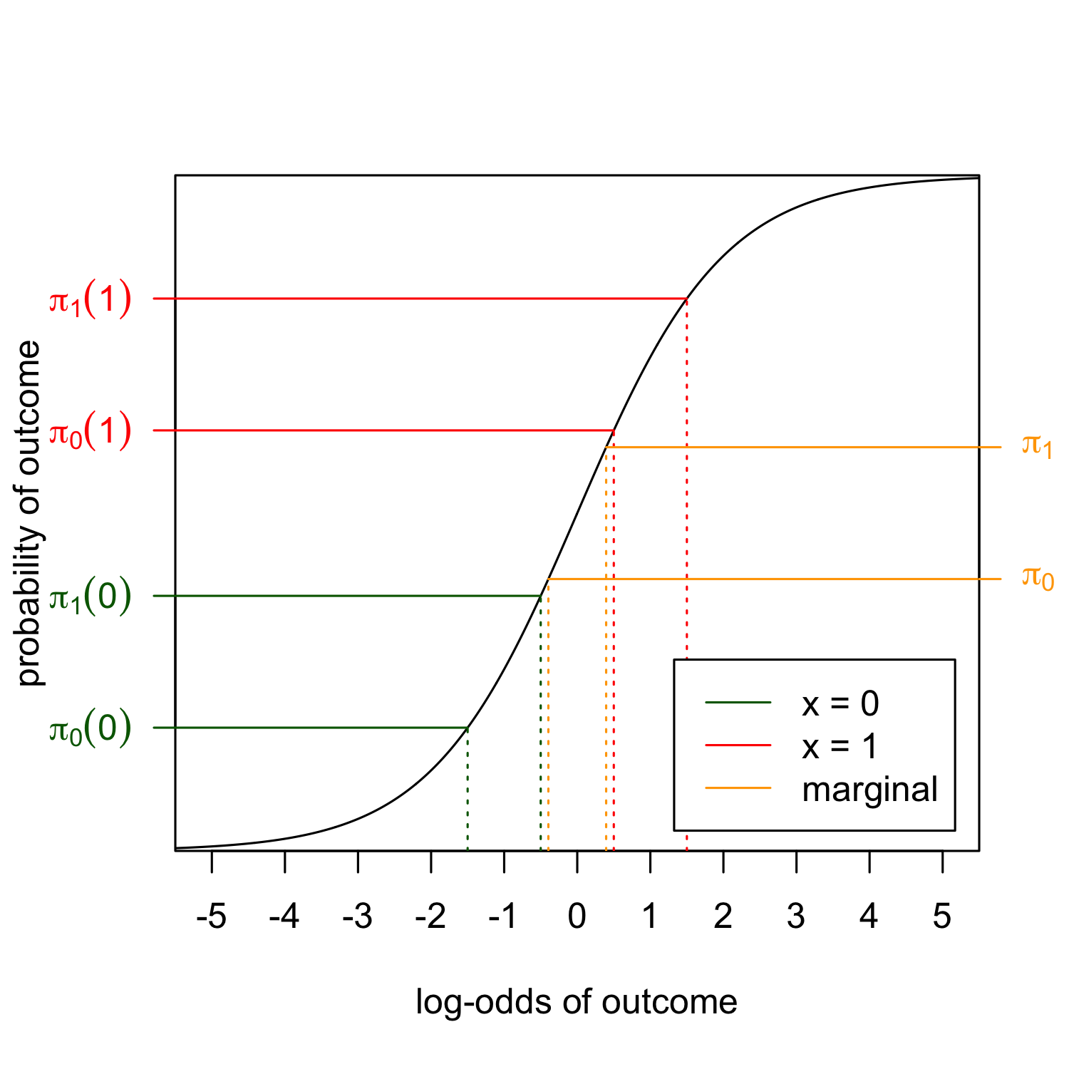
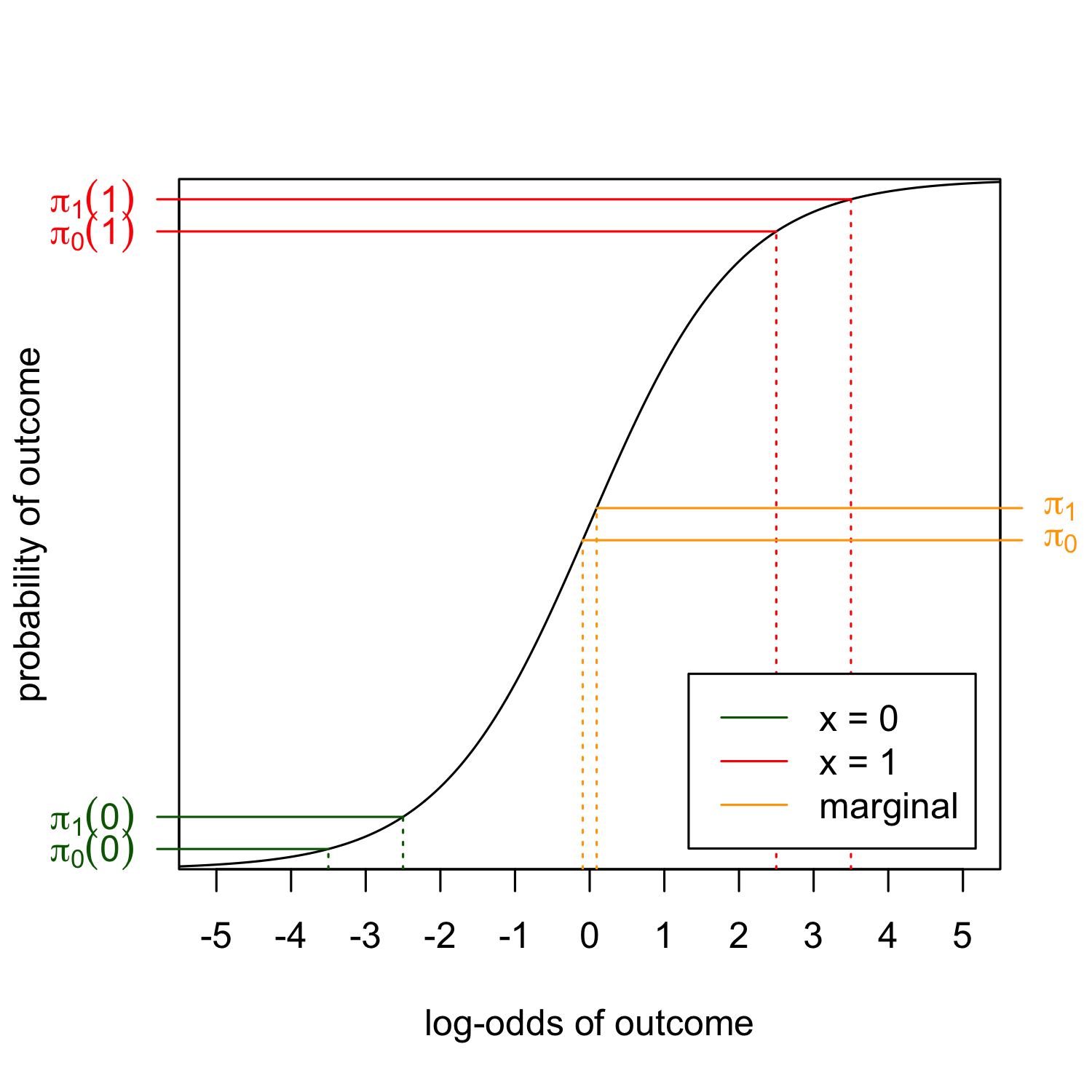
Figure 3: Illustration of non-collapsibility. For fixed $p(x=1)=0.5$ and $\beta_{t}=1.0$, the marginal log odds-ratio $\gamma$ of treatment becomes closer to $0$ when the difference in the untreated risks $\pi_{0}(0),\pi_{0}(1)$ becomes larger.

A.2 Consistency of marginally constrained models

Here we prove Theorem 1. First we state the formal version of the theorem:

Theorem 1.

(formal version) Given binary treatment $T$, binary outcome $Y$ and covariate $X$. Assume strong ignorability $(Y_{1},Y_{0})\perp\!\!\!\perp T|X$, positivity $0<q(T|X)<1$ and consistency $Y_{t}=Y$ if $T=t$. Given a model $p_{\theta}(y|t,x)$ indexed by parameter $\theta\in\Theta$, and assuming $\exists\theta^{*}\in\Theta,\Pr(Y_{t}=1|X=x)=p_{\theta^{*}}(y|t,x)$. Denote the sample log-likelihood $L_{n}:\Theta\to\mathbb{R}$, marginal log odds-ratio $\gamma=\sigma^{-1}(\Pr(Y_{1}=1))-\sigma^{-1}(\Pr(Y_{0}=1))$, sample marginalizer $M_{n}:\Theta\to\mathbb{R}$:

$$M_{n}(\theta)=\sigma^{-1}(\frac{1}{n}\sum_{i=1}^{n}p_{\theta}(Y=1|1,x_{i}))-\sigma^{-1}(\frac{1}{n}\sum_{i=1}^{n}p_{\theta}(Y=1|0,x_{i}))$$ (16)

and $0<\lambda<\infty$. Assume that $L_{n}$ converges uniformly in probability to $L:\Theta\to\mathbb{R}$ and $M_{n}$ to $M:\Theta\to\mathbb{R}:$

$$M(\theta)=\sigma^{-1}(\operatorname{\mathbb{E}}p_{\theta}(Y=1|1,X))-\sigma^{-1}(\operatorname{\mathbb{E}}p_{\theta}(Y=1|0,X))$$ (17)

The uniform convergence in probability means:

$$\sup_{\theta\in\Theta}|L_{n}(\theta)-L(\theta)| \overset{p}{\to}0$$

$$\sup_{\theta\in\Theta}|M_{n}(\theta)-M(\theta)| \overset{p}{\to}0$$

Additionally, assume strong identifiability, namely that for every $\epsilon>0$ the Kullback-Leibler (KL) divergence between the data distribution and model distribution:

$$\inf_{\theta:|\theta-\theta^{*}|\geq\epsilon}\text{KL}(p_{\theta^{*}}(y|t,x),p_{\theta}(y|t,x))>0$$

Then:

$$\theta_{n}=\arg\max_{\theta\in\Theta}\left[L_{n}(\theta)-\lambda(M_{n}(\theta)-\gamma)^{2}\right]$$

is a consistent estimator of $\theta^{*}$ so the model matches $\Pr(Y_{t}=1|X)$

To prove this theorem we first prove that $\Pr(Y_{t}=1|X)=\Pr(Y|T,X)$ (causal identifiability) and then consistency of the constrained estimator for the observational distribution.

Proof.

A standard causal inference result is that under strong ignorability, positivity and (causal) consistency, $\Pr(Y_{t}=1|X)=\Pr(Y=1|T,X)$. Restating the proof:

$$\Pr(Y_{t}=1|X) =\Pr(Y_{t}=1|X,t)$$

$$=\Pr(Y=1|X,t)$$

The first equality follows from the strong ingorability assumption $(Y_{0},Y_{1})\perp\!\!\!\perp T|X$, the second follows from the consistency assumption $Y_{t}=Y,T=t$. The right hand side now only contains observable quantities. We now prove that the constrained estimator is a consistent estimator of $\Pr(Y_{t}=1|X)$.

Writing the population objective and its empirical counterpart:

$$\mathcal{L}(\theta) =\operatorname{\mathbb{E}}\log p_{\theta}(y_{i}|x_{i},t_{i})-\lambda(M(\theta)-\gamma)^{2}$$ (18)

$$\mathcal{L}_{n}(\theta) =\frac{1}{n}\sum_{i=1}^{n}\log p_{\theta}(y_{i}|x_{i},t_{i})-\lambda(M_{n}(\theta)-\gamma)^{2}$$ (19)

We first introduce a new objective:

$$R_{n}^{\theta^{*}}(\theta) =\mathcal{L}_{n}(\theta^{*})-\mathcal{L}_{n}(\theta)$$ (20)

$$=\frac{1}{n}\sum_{i=1}^{n}\log\frac{p_{\theta^{*}}(y_{i}|x_{i},t_{i})}{p_{\theta}(y_{i}|x_{i},t_{i})}-\lambda(M_{n}(\theta^{*})-\gamma)^{2}+\lambda(M_{n}(\theta)-\gamma)^{2}$$ (21)

Because the first term in 20 is constant it is clear that

$$\hat{\theta}=\arg\min_{\theta\in\Theta}R_{n}(\theta)\Longleftrightarrow\hat{\theta}=\arg\max_{\theta\in\Theta}\mathcal{L}_{n}(\theta)$$

The population version of $R_{n}^{\theta^{*}}$ is:

$$R^{\theta^{*}}(\theta) =\operatorname{\mathbb{E}}_{t,x}\operatorname{\mathbb{E}}_{y|t,x}\log\frac{p_{\theta^{*}}(y|x,t)}{p_{\theta}(y|x,t)}-\lambda(M(\theta^{*})-\gamma)^{2}+\lambda(M(\theta)-\gamma)^{2}$$ (22)

$$\overset{(i)}{=}\operatorname{\mathbb{E}}_{t,x}\text{KL}(p_{\theta^{*}}(y|x,t)||p_{\theta}(y|x,t))-\lambda(M(\theta^{*})-\gamma)^{2}+\lambda(M(\theta)-\gamma)^{2}$$ (23)

$$\overset{(ii)}{=}\operatorname{\mathbb{E}}_{t,x}\text{KL}(p_{\theta^{*}}(y|x,t)||p_{\theta}(y|x,t))+\lambda(M(\theta)-\gamma)^{2}$$ (24)

Where $(i)$ is substituting the definition of the KL-divergence and equality $(ii)$ holds as $\gamma=M(\theta^{*})$ by definition.

Lemma 3 gives that uniform convergence in probability of $L_{n}$ and $M_{n}$ imply uniform convergence in probability of $\mathcal{L}_{n}$ and thus $R_{n}$ as $R_{n}$ is just a constant minus $\mathcal{L}_{n}$. We now use this convergence to prove that $R_{n}^{\theta^{*}}\overset{p}{\to}0$ as $n\to\infty$, which will prove the consistency of the constrained estimator. Denote $\hat{\theta}_{n}$ as the maximizer of $\mathcal{L}_{n}$, because of this, it must be that

$$R_{n}^{\theta^{*}}(\hat{\theta}_{n})=\mathcal{L}_{n}(\theta^{*})-\mathcal{L}_{n}(\hat{\theta}_{n})\leq 0$$

We can now bound $R^{\theta^{*}}(\hat{\theta}_{n})$ and show that it converges to $0$ in probability:

$$R^{\theta^{*}}(\hat{\theta}_{n})=R^{\theta^{*}}(\hat{\theta}_{n})-R_{n}^{\theta^{*}}(\hat{\theta}_{n})+R_{n}^{\theta^{*}}(\hat{\theta}_{n})\overset{(i)}{\leq}R^{\theta^{*}}(\hat{\theta}_{n})-R_{n}^{\theta^{*}}(\hat{\theta}_{n})\overset{p}{\to}0$$ (25)

The inequality $(i)$ holds as $R_{n}^{\theta}(\hat{\theta})\leq 0$ and the convergence is given by uniform convergence of $R_{n}$. To show that the KL-divergence goes to zero, note that:

$$R^{\theta^{*}}(\hat{\theta}_{n}) =\underbrace{\operatorname{\mathbb{E}}_{t,x}\text{KL}(p_{\theta^{*}}(y|x,t)||p_{\hat{\theta}_{n}}(y|x,t))}_{A_{n}}+\underbrace{\lambda(M(\hat{\theta}_{n})-\gamma)^{2}}_{B_{n}}\overset{p}{\to}0$$ (26)

$A_{n}$ is non-negative because the KL-divergence is non-negative and $B_{n}$ is non-negative as well. For all $n$, $A_{n}$ is lower bounded by $0$ and upper bounded by $R_{n}$, by application of the squeeze theorem adapted for convergence in probability, $R_{n}\overset{p}{\to}0\implies A_{n}\overset{p}{\to}0$. For a short proof on how the squeeze theorem for sequences translates to convergence in probability, see Lemma 4 below. The assumption of strong identifiability gaurantees that $\theta\to\theta^{*}$ as the KL-divergence goes to zero, proving the consistency of the constrained estimator.

∎

Lemma 1.

Let $A_{n}(\theta),B_{n}(\theta)\in\mathbb{R}$ be sequences of real-valued random variables for parameter $\theta$ and $A(\theta),B(\theta)$ be random variables in $\mathbb{R}$. If both

$$\sup_{\theta}|A_{n}(\theta)-A(\theta)| \overset{p}{\to}0$$

$$\sup_{\theta}|B_{n}(\theta)-B(\theta)| \overset{p}{\to}0$$ (27)

then,

$$\sup_{\theta}|A_{n}(\theta)+B_{n}(\theta)-A(\theta)-B(\theta)| \overset{p}{\to}0.$$

Proof.

Define $C_{n}(\theta)=A_{n}(\theta)-A(\theta)$ and $D_{n}(\theta)=B_{n}(\theta)-B(\theta)$. By the definition of convergence in probability, the goal is to show that

$$\lim_{n\to\infty}\Pr(\sup_{\theta}|C_{n}(\theta)+D_{n}(\theta|>\epsilon)=0$$

Now construct an upper bound on the probability

$$\Pr(\sup_{\theta}|C_{n}(\theta)+D_{n}(\theta)|>\epsilon)$$

$$\leq\Pr(\sup_{\theta}|C_{n}(\theta)|+|D_{n}(\theta)|>\epsilon)$$

$$\leq\Pr(\sup_{\theta_{C}}|C_{n}(\theta_{C})|+\sup_{\theta_{D}}|D_{n}(\theta_{D})|>\epsilon)$$

$$\leq\Pr(\sup_{\theta_{C}}|C_{n}(\theta_{C})|>\nicefrac{{\epsilon}}{{2}}\quad\text{or}\quad\sup_{\theta_{D}}|D_{n}(\theta_{D})|>\nicefrac{{\epsilon}}{{2}})$$ (28)

$$\leq\Pr(\sup_{\theta}|C_{n}(\theta)|>\nicefrac{{\epsilon}}{{2}})+\Pr(\sup_{\theta}|D_{n}(\theta)|>\nicefrac{{\epsilon}}{{2}})$$

$$=\Pr(\sup_{\theta}|A_{n}(\theta)-A(\theta)|>\nicefrac{{\epsilon}}{{2}})+\Pr(\sup_{\theta}|B_{n}(\theta)-B(\theta)|>\nicefrac{{\epsilon}}{{2}}).$$ (29)

By the assumption of convergence in probability in Equation 27,

$$\lim_{n\to\infty}\Pr(\sup_{\theta}|A_{n}(\theta)-A(\theta)|>\nicefrac{{\epsilon}}{{2}})+\Pr(\sup_{\theta}|B_{n}(\theta)-B(\theta)|>\nicefrac{{\epsilon}}{{2}})=0.$$

This limit shows that $\Pr(\sup_{\theta}|C_{n}(\theta)+D_{n}(\theta)|>\epsilon)$ goes to zero via the squeeze theorem because the upper bound, Equation 29, goes to zero and the lower bound on probabilities of zero, thus showing the desired convergence in probability. ∎

Lemma 2.

Let $M_{n}(\theta)\in\mathbb{R}$ be a sequence of real-valued random variables for parameter $\theta\in\Theta$ and $M(\theta),\gamma\in\mathbb{R}$ for $\theta\in\Theta$. If $\sup_{\theta\in\Theta}|M_{n}(\theta)-M(\theta)|\overset{p}{\to}0$ then $\sup_{\theta\in\Theta}|(M_{n}(\theta)-\gamma)^{2}-(M(\theta)-\gamma)^{2}|\overset{p}{\to}0$

Proof.

Define $\xi_{n}(\theta)=M_{n}(\theta)-M(\theta)$, then:

$$\sup_{\theta\in\Theta}|M_{n}(\theta)-M(\theta)|\overset{p}{\to}0\implies\sup_{\theta\in\Theta}|\xi_{n}(\theta)|\overset{p}{\to}0$$ (30)

We have that

$$(M_{n}-\gamma)^{2}-(M-\gamma)^{2}= (M+\xi_{n}-\gamma)^{2}-(M-\gamma)^{2}$$ (31)

$$= M^{2}+\xi_{n}^{2}+\gamma^{2}+2M\xi_{n}-2\gamma\xi_{n}-2M\gamma$$ (32)

$$-M^{2}-\gamma^{2}+2M\gamma$$ (33)

$$= \xi_{n}^{2}+2\xi_{n}(M-\gamma)$$ (34)

We need to show that

$$\Pr(\sup_{\theta\in\Theta}|\xi_{n}(\theta)^{2}+2\xi_{n}(\theta)(M(\theta)-\gamma)|>\epsilon)\underset{n\to\infty}{=}0$$

This expression is the sum of two sequences with $\xi_{n}$. By Lemma 1, our desired result follows if both:

$$\sup_{\theta\in\Theta}|\xi_{n}(\theta)^{2}| \overset{p}{\to}0$$

$$\sup_{\theta\in\Theta}|2\xi_{n}(\theta)(M(\theta)-\gamma)| \overset{p}{\to}0$$

We can bound the term with $\xi_{n}$ using 30 and the fact that $M(\theta)-\gamma\in\mathbb{R},\forall\theta\in\Theta$. For $|\xi_{n}|^{2}$ to converge to $0$, note that:

$$\Pr(\sup_{\theta\in\Theta}|\xi_{n}(\theta)|^{2}>\epsilon)=\Pr(\sup_{\theta\in\Theta}[|\xi_{n}(\theta)||\xi_{n}(\theta)|]>\epsilon)=\Pr(\sup_{\theta\in\Theta}|\xi_{n}(\theta)|>\sqrt{\epsilon})$$

Again, applying 30 gives the required result. ∎

Lemma 3.

Let $L_{n}(\theta),M_{n}(\theta)\in\mathbb{R}$ be sequences of real-valued random variables for $\theta\in\Theta$ and $L(\theta),M(\theta),\gamma\in\mathbb{R}$, and let $0<\lambda<\infty$. Define

$$\mathcal{L}_{n} =L_{n}-\lambda(M_{n}-\gamma)^{2}$$

$$\mathcal{L} =L-\lambda(M-\gamma)^{2}$$

Then if $L_{n}\overset{p}{\to}L$ uniformly and $M_{n}\overset{p}{\to}M$ uniformly, then $\mathcal{L}_{n}\overset{p}{\to}\mathcal{L}$ uniformly

Proof.

By Lemma 2 we have that

$$\sup_{\theta}|M_{n}(\theta)-M(\theta)|\overset{p}{\to}0\implies\sup_{\theta\in\Theta}|(M_{n}(\theta)-\gamma)^{2}-(M(\theta)-\gamma)^{2}|\overset{p}{\to}0$$

By uniform convergence in probability we have that also

$$\sup_{\theta}|L_{n}(\theta)-L(\theta)| \overset{p}{\to}0$$

This gives us

$$\sup_{\theta}|\mathcal{L}_{n}(\theta)-\mathcal{L}(\theta)| =\sup_{\theta}|L_{n}(\theta)-\lambda(M_{n}(\theta)-\gamma)^{2}-L+\lambda(M(\theta)-\gamma)^{2}|$$

$$\overset{i}{\leq}\sup_{\theta}|L_{n}(\theta)-L(\theta)|+\lambda\sup_{\theta}|(M(\theta)-\gamma)^{2}-(M_{n}(\theta)-\gamma)^{2}|\overset{p}{\to}0$$

$(i)$ follows from the triangle inequality and the final convergence follows from $0<\lambda<\infty$ and the uniform convergence of the individual terms. ∎

Lemma 4.

If $X_{n}\leq Y_{n}\leq Z_{n}$ for every $n$ and $X_{n}\overset{p}{\to}L$ and $Z_{n}\overset{p}{\to}L$, then $Y_{n}\overset{p}{\to}L$

Proof.

We want to show that for any $\epsilon>0$, we have

$$\lim_{n\to\infty}\Pr(|Y_{n}-L|>\epsilon)=0$$

Note that

$$X_{n}\leq Y_{n}\leq Z_{n}$$

implies

$$|Y_{n}-L|\leq|X_{n}-L|+|Z_{n}-L|$$

so

$$\Pr(|Y_{n}-L|>\epsilon)\leq\Pr(|X_{n}-L|+|Z_{n}-L|>\epsilon)$$

The right-hand side can be made arbitrarily small by convergence of $X_{n}$ and $Z_{n}$, proving what we want to show. ∎

A.3 The offset model is not a consistent estimator in the presence of unobserved confounding

We now prove that optimization over the offset model family in Equation 7 and a known conditional odds-ratio $\beta_{t}$ leads to an asymptotically biased estimator of $\Pr(Y_{t}|x)$ in the presence of unobserved confounding in a simple example introduced in the main text (4.1). In this example, $\Pr(Y_{t}|x)=\Pr(Y_{t})$, or equivalently, there is no covariate $X$. This also implies that here CATE=ATE, so we will use ATE instead. Given the offset model family from Equation 7, a natural parameterization of $g(t,x)=g(t)$ in the context of this example is $g(t;b_{0})=\sigma(b_{0}+\beta_{t}t),b_{0}\in\mathbb{R}$. Again, we are assuming that $\beta_{t}$ is given a-priori and is not estimated. We first derive an expression for the expected log-likelihood as a function of $b_{0}$ under the observational distribution in this example. Then we show that the ground truth solution $\beta_{0}$ is not a stationary point, proving our claim. Writing

$$p_{u}= p(u=1)$$

$$p_{{t}^{\prime}u^{\prime}}= p({t}={t}^{\prime},u=u^{\prime})=p({t}={t}^{\prime}|u=u^{\prime})p(u=u^{\prime})$$

$$\pi_{{t}^{\prime}u^{\prime}}= p(y=1|{t}={t}^{\prime},u=u^{\prime})$$

Then the data generating mechanism is:

$$t,u\sim\mathcal{B}(p_{{t}^{\prime}u^{\prime}}),y\sim\mathcal{B}(\pi_{{t}u})$$

The ground truth solutions $\beta_{0}$ and $\beta_{t}$ are:

$$\Pr(Y_{0}=1) =(1-p_{u})\pi_{00}+p_{u}\pi_{01}=\sigma(\beta_{0})$$ (35)

$$\Pr(Y_{1}=1) =(1-p_{u})\pi_{10}+p_{u}\pi_{11}=\sigma(\beta_{0}+\beta_{t})$$ (36)

The Bernoulli log-likelihood is

$$l(y|{t},b_{0})=y\log\sigma(b_{0}+\beta_{t}{t})+(1-y)\log(1-\sigma(b_{0}+\beta_{t}t))$$

In offset models $\beta_{t}$ is assumed given a priori and $b_{0}$ is the only parameter, resulting in the following expression for $L(b_{0})$:

$$L(b_{0})= p_{00}\left[\pi_{00}\log\sigma(b_{0})+(1-\pi_{00})\log(1-\sigma(b_{0}))\right]$$

$$+ p_{01}\left[\pi_{01}\log\sigma(b_{0})+(1-\pi_{01})\log(1-\sigma(b_{0}))\right]$$

$$+ p_{10}\left[\pi_{10}\log\sigma(b_{0}+\beta_{t})+(1-\pi_{10})\log(1-\sigma(b_{0}+\beta_{t}))\right]$$

$$+ p_{11}\left[\pi_{11}\log\sigma(b_{0}+\beta_{t})+(1-\pi_{11})\log(1-\sigma(b_{0}+\beta_{t}))\right]$$

Taking the derivative with respect to $b_{0}$, noting that $(\log\sigma(x))^{\prime}=1-\sigma(x)$, we get:

$$\frac{\partial L}{\partial b_{0}}= p_{00}\left[\pi_{00}(1-\sigma(b_{0}))-(1-\pi_{00})\sigma(b_{0})\right]$$ (37)

$$+ p_{01}\left[\pi_{01}(1-\sigma(b_{0}))-(1-\pi_{01})\sigma(b_{0})\right]$$

$$+ p_{10}\left[\pi_{10}(1-\sigma(b_{0}+\beta_{t}))-(1-\pi_{10})\sigma(b_{0}+\beta_{t})\right]$$

$$+ p_{11}\left[\pi_{11}(1-\sigma(b_{0}+\beta_{t}))-(1-\pi_{11})\sigma(b_{0}+\beta_{t})\right]$$

We now plug in the ground truth solutions for $\beta_{0},\beta_{t}$ (Equations 35).

$$\frac{\partial L}{\partial b_{0}}(b_{0}=\beta_{0})= p_{00}\left[\pi_{00}(1-p_{u}\pi_{01}-(1-p_{u})\pi_{00})-(1-\pi_{00})(p_{u}\pi_{01}+(1-p_{u})\pi_{00})\right]$$

$$+ p_{01}\left[\pi_{01}(1-p_{u}\pi_{01}-(1-p_{u})\pi_{00})-(1-\pi_{01})(p_{u}\pi_{01}+(1-p_{u})\pi_{00})\right]$$

$$+ p_{10}\left[\pi_{10}(1-p_{u}\pi_{11}-(1-p_{u})\pi_{10})-(1-\pi_{10})(p_{u}\pi_{11}+(1-p_{u})\pi_{10})\right]$$

$$+ p_{11}\left[\pi_{11}(1-p_{u}\pi_{11}-(1-p_{u})\pi_{10})-(1-\pi_{11})(p_{u}\pi_{11}+(1-p_{u})\pi_{10})\right]$$

Removing terms that cancel out in each line results in

$$\frac{\partial L}{\partial b_{0}}(b_{0}=\beta_{0})= p_{00}\left[p_{u}(\pi_{00}-\pi_{01})\right]$$

$$+ p_{01}\left[(1-p_{u})(\pi_{01}-\pi_{00})\right]$$

$$+ p_{10}\left[p_{u}(\pi_{10}-\pi_{11})\right]$$

$$+ p_{11}\left[(1-p_{u})(\pi_{11}-\pi_{10})\right]$$

Substituting back $p_{{t}^{\prime}u^{\prime}}=p({t}={t}^{\prime}|u=u^{\prime})p(u=u^{\prime})$:

$$\frac{\partial L}{\partial b_{0}}(b_{0}=\beta_{0})= p({t}=0|u=0)(1-p_{u})\left[p_{u}(\pi_{00}-\pi_{01})\right]$$

$$+ p({t}=0|u=1)p_{u}\left[(1-p_{u})(\pi_{01}-\pi_{00})\right]$$

$$+ p({t}=1|u=0)(1-p_{u})\left[p_{u}(\pi_{10}-\pi_{11})\right]$$

$$+ p({t}=1|u=1)p_{u}\left[(1-p_{u})(\pi_{11}-\pi_{10})\right]$$

Factoring out $p_{u}(1-p_{u})$ and re-arranging we arrive at our result:

$$\frac{\partial L}{\partial b_{0}}(b_{0}=\beta_{0})=p_{u}(1-p_{u})\bigl{[} (\pi_{01}-\pi_{00})\left(p({t}=0|u=1)-p({t}=0|u=0)\right)+$$

$$(\pi_{11}-\pi_{10})\left(p({t}=1|u=1)-p({t}=1|u=0)\right)\bigr{]}$$

If there is no confounding ($\pi_{t0}=\pi_{t1}$ or $p(t|u=0)=p(t|u=1)$) this expression is zero, but in general it is not which means that the ground truth solution $\beta_{0}$ is not an optimum of the expected log-likelihood in the observational data distribution. This proves our claim that the offset model does not recover $\Pr(Y_{t})$ in the presence of confounding. $\square$

Of note, the fact that the offset model does not estimate $\Pr(Y_{t})$ does not automatically imply that the ATE is not correctly estimated as there may be another $b_{0}^{\prime}\neq\beta_{0}$ such that $\widehat{\text{ATE}}(b_{0}=b_{0}^{\prime})={\text{ATE}}(b_{0}=\beta_{0})$. To investigate this, assume that for some $\beta_{0}=a$ and $\beta_{t}=c$ we have that:

$$\delta:= \sigma(a+c)-\sigma(a)$$

$$= \frac{e^{a+c}}{1+e^{a+c}}-\frac{e^{a}}{1+e^{a}}$$

Again, treating $\beta_{t}$ as fixed, we will now prove that this equation has at most two solutions for $b_{0}=a$ by noting that:

$$\frac{e^{a+c}}{1+e^{a+c}}-\frac{e^{a}}{1+e^{a}} =\frac{e^{a+c}(1+e^{a})-(1+e^{a+c})e^{a}}{(1+e^{a+c})(1+e^{a})}$$

$$=\frac{e^{a}(e^{c}-1)}{(1+e^{a+c})(1+e^{a})}$$

Introducing $y:=e^{a}$ and cross-multiplying we get:

$$\delta =\frac{y(e^{c}-1)}{(1+e^{c}y)(1+y)}\iff$$

$$\delta(1+e^{c}y)(1+y) =y(e^{c}-1)=$$

$$\delta+\delta(1+e^{c})y+\delta e^{c}y^{2} =y(e^{c}-1)\iff$$

$$\delta e^{c}y^{2}+\left(\delta(1+e^{c})-e^{c}+1\right)y+\delta =0$$

Depending on the values of $\delta$ and $c$ this quadratic equation in $y$ has 0, 1 or 2 real-valued solutions, yielding 0, 1 or 2 real-valued solutions for $a=\log y=b_{0}$. This implies that there exists utmost one alternative solution $b_{0}^{\prime}\neq\beta_{0}$ such that $\widehat{\text{ATE}}(b_{0}=b_{0}^{\prime})={\text{ATE}}(b_{0}=\beta_{0})$.

In fact, we can explicitly compute this alternative solution by exploiting the symmetry of the sigmoid function: $\sigma(x)=1-\sigma(-x)$. Whenever it is true that:

$$\sigma(\beta_{0}+\beta_{t})-\sigma(\beta_{0})=\delta$$

It must simultaneously be true that, writing $\beta^{\prime}_{0}:=-(\beta_{0}+\beta_{t})$:

$$\sigma(\beta^{\prime}_{0}+\beta_{t})-\sigma(\beta^{\prime}_{0}) =$$

$$\sigma(-(\beta_{0}+\beta_{t})+\beta_{t})-\sigma(-(\beta_{0}+\beta_{t})) =$$

$$\sigma(-\beta_{0})-\sigma(-(\beta_{0}+\beta_{t})) =$$

$$(1-\sigma(\beta_{0}))-(1-\sigma(\beta_{0}+\beta_{t})) =$$

$$\sigma(\beta_{0}+\beta_{t})-\sigma(\beta_{0}) =\delta$$

This means that except in the trivial case when $\beta_{0}=\beta_{t}=0$ there always exists a second solution $\beta^{\prime}_{0}$ that has the same ATE $\delta$ but a different $\Pr(Y_{t})$. We can check whether this coincidentally coincides with the maximum likelihood solution for $b_{0}$ in the offset model on the observational data by plugging in $\beta^{\prime}_{0}:=-(\beta_{0}+\beta_{t})$ in the expression of the gradient of the likelihood (Equation 37). Again we remove terms that cancel out and substitute back $p_{{t}^{\prime}u^{\prime}}=p({t}={t}^{\prime}|u=u^{\prime})p(u=u^{\prime})$ to arrive at:

$$\frac{\partial L}{\partial b_{0}}(b_{0}=\beta^{\prime}_{0}) =p_{u}(1-p_{u})\bigl{(}p({t}=0|u=1)-p({t}=0|u=0)\bigr{)}\bigl{(}(\pi_{10}-\pi_{11})+(\pi_{01}-\pi_{00})\bigr{)}$$ (38)

$$+p_{u}\bigl{(}(\pi_{11}-\pi_{10})+(\pi_{01}-\pi_{00})\bigr{)}$$ (39)

$$+2\pi_{10}+\pi_{11}-1$$ (40)

Analyzing this expression line-by-line we see that the first two lines are non-zero in general when there is confounding such that $p({t}=0|u=1)\neq p({t}=0|u=0)$ and $\pi_{{t}1}\neq\pi_{{t}0}$. The last line is also non-zero in general as $\pi_{{t}u}$ are free parameters. This shows that the offset model is also an asymptotically biased estimator of the ATE.

A.4 Analytical solution of offset model with binary covariate

Assume a binary treatment $t$, covariate $x$ and outcome $y$. Write:

$$\beta_{t}^{0} =\sigma^{-1}(\Pr(Y_{1}=1|x=0))-\sigma^{-1}(\Pr(Y_{0}=1|x=0))$$ (41)

$$\beta_{t}^{1} =\sigma^{-1}(\Pr(Y_{1}=1|x=1))-\sigma^{-1}(\Pr(Y_{0}=1|x=1))$$ (42)

The offset assumption states that $\beta_{t}^{0}=\beta_{t}^{1}=\beta_{t}$.

A.4.1 Offset solution

Maximizing the likelihood over a model class is equivalent to minimizing the Kullback-Leibler divergence between the actual distribution and the model distribution. We find an analytical solution for the offset models by writing the estimation objective as minimizing the Kullback-Leibler divergence between the model distribution and the observed data distribution with the additional constraints above 41. Writing:

• $p_{tx}$ for estimated probabilities of $\Pr(Y=1|t,x)$, such that $p(y|t,x)=(1-y)(1-p_{tx})+yp_{tx}$

• $q_{tx}$ for actual (observational) probabilities of $\Pr(Y=1|t,x)$, such that $q(y|t,x)=(1-y)(1-q_{tx})+yq_{tx}$

• $q(t,x)=\Pr(T=t,X=x)$, the observational joint probability of $T,X$

The criterion is:

$$L =\operatorname{\mathbb{E}}_{t,x}\operatorname{\mathbb{E}}_{y|t,x}\log\frac{q(y|t,x)}{p(y|t,x)}+\lambda_{0}\left(\sigma^{-1}(p_{10})-\sigma^{-1}(p_{00})-\beta_{t}\right)+\lambda_{1}\left(\sigma^{-1}(p_{11})-\sigma^{-1}(p_{01})-\beta_{t}\right)$$ (43)

The partial derivatives for all parameters $(p_{00},p_{01},p_{10},p_{11},\lambda_{0},\lambda_{1})$ are:

$$\frac{\partial L}{\partial p_{00}} =\operatorname{\mathbb{E}}_{t,x}\operatorname{\mathbb{E}}_{y|t,x}\frac{\partial}{\partial p_{00}}\left[\left(\log q(y|t,x)-\log p(y|t,x)\right)+\lambda_{0}\left(\sigma^{-1}(p_{10})-\sigma^{-1}(p_{00})-\beta_{t}\right)+\lambda_{1}\left(\sigma^{-1}(p_{11})-\sigma^{-1}(p_{01})-\beta_{t}\right)\right]$$ (44)

$$=\operatorname{\mathbb{E}}_{t,x}\operatorname{\mathbb{E}}_{y|t,x}\frac{\partial}{\partial p_{00}}\left[\left(\log q(y|t,x)-\log(yp_{tx}+(1-y)(1-p_{tx})\right)\right]-\lambda_{0}\frac{\partial}{\partial p_{00}}\sigma^{-1}(p_{00})$$ (45)

$$=q(0,0)\left[(1-q_{00})\frac{1}{1-p_{00}}-q_{00}\frac{1}{p_{00}}\right]-\lambda_{0}\left(\frac{1}{p_{00}}+\frac{1}{1-p_{00}}\right)$$ (46)

$$=q(0,0)\left[\frac{(1-q_{00})p_{00}-q_{00}(1-p_{00})}{p_{00}(1-p_{00})}\right]-\lambda_{0}\left(\frac{(1-p_{00})+p_{00}}{p_{00}(1-p_{00})}\right)$$ (47)

$$=q(0,0)\left[\frac{p_{00}-q_{00}}{p_{00}(1-p_{00})}\right]-\lambda_{0}\left(\frac{1}{p_{00}(1-p_{00})}\right)$$ (48)

$$=\frac{q(0,0)\left(p_{00}-q_{00}\right)-\lambda_{0}}{p_{00}(1-p_{00})}$$ (49)

$$\frac{\partial L}{\partial p_{01}} =\frac{q(0,1)\left(p_{01}-q_{01}\right)-\lambda_{1}}{p_{01}(1-p_{01})}$$ (50)

$$\frac{\partial L}{\partial p_{10}} =\frac{q(1,0)\left(p_{10}-q_{10}\right)+\lambda_{0}}{p_{10}(1-p_{10})}$$ (51)

$$\frac{\partial L}{\partial p_{11}} =\frac{q(1,1)\left(p_{11}-q_{11}\right)+\lambda_{1}}{p_{11}(1-p_{11})}$$ (52)

$$\frac{\partial L}{\partial\lambda_{0}} =\sigma^{-1}(p_{10})-\sigma^{-1}(p_{00})-\beta_{t}$$ (53)

$$\frac{\partial L}{\partial\lambda_{1}} =\sigma^{-1}(p_{11})-\sigma^{-1}(p_{01})-\beta_{t}$$ (54)

Setting the gradient to zero to find an extremum of 43 and requiring $0<p_{tx}<1$ we get:

$0=$

1. $q(0,0)\left(p_{00}-q_{00}\right)-\lambda_{0}$

2. $q(0,1)\left(p_{01}-q_{01}\right)-\lambda_{1}$

3. $q(1,0)\left(p_{10}-q_{10}\right)+\lambda_{0}$

4. $q(1,1)\left(p_{11}-q_{11}\right)+\lambda_{1}$

5. $\sigma^{-1}(p_{10})-\sigma^{-1}(p_{00})-\beta_{t}$

6. $\sigma^{-1}(p_{11})-\sigma^{-1}(p_{01})-\beta_{t}$

Combining (a) and (c):

$$a+c =q(0,0)(p_{00}-q_{00})+q(1,0)(p_{10}-q_{10})-\lambda_{0}+\lambda_{0}=0$$ (56)

$$0 =q(0,0)(p_{00}-q_{00})+q(1,0)(p_{10}-q_{10})$$ (57)

Inserting (e): $p_{10}=\sigma\left(\sigma^{-1}(p_{00})+\beta_{t}\right)$ we get

$$0 =q(0,0)(p_{00}-q_{00})+q(1,0)(\sigma\left(\sigma^{-1}(p_{00})+\beta_{t}\right)-q_{10})$$ (58)

Using $\sigma\left(\sigma^{-1}(x)+a\right)=\frac{e^{a}x}{(e^{a}-1)x+1}$ we get:

$$0 =q(0,0)(p_{00}-q_{00})+q(1,0)\left(\frac{e^{\beta_{t}}p_{00}}{(e^{\beta_{t}}-1)p_{00}+1)}-q_{10}\right)$$ (60)

By multiplying both sides with $(e^{\beta_{t}}-1)p_{00}+1$ we end up with a quadratic equation in $p_{00}$. Using some intermediate variables to shorten the notation and applying the same steps to get $p_{01}$, the solution is:

$$\tau =e^{\beta_{t}}$$

$$r_{x} =q(1,x)/q(0,x)$$

$$c_{x} =-(q(y|0,x)+r_{x}q(y|1,x))$$

$$b_{x} =1+r_{x}\tau+c_{x}(\tau-1)$$

$$p_{0x} =\frac{-b_{x}\pm\sqrt{b_{x}^{2}+4(\tau-1)c_{x}}}{2(\tau-1)}$$

The $\pm$ solution is taken to equal sign$(\beta_{t})$. Without loss of generality we assume $\beta_{t}>0$. The corresponding solutions $p_{1x}$ are given by $p_{1x}=\sigma(\sigma^{-1}(p_{0x})+\beta_{t})$.

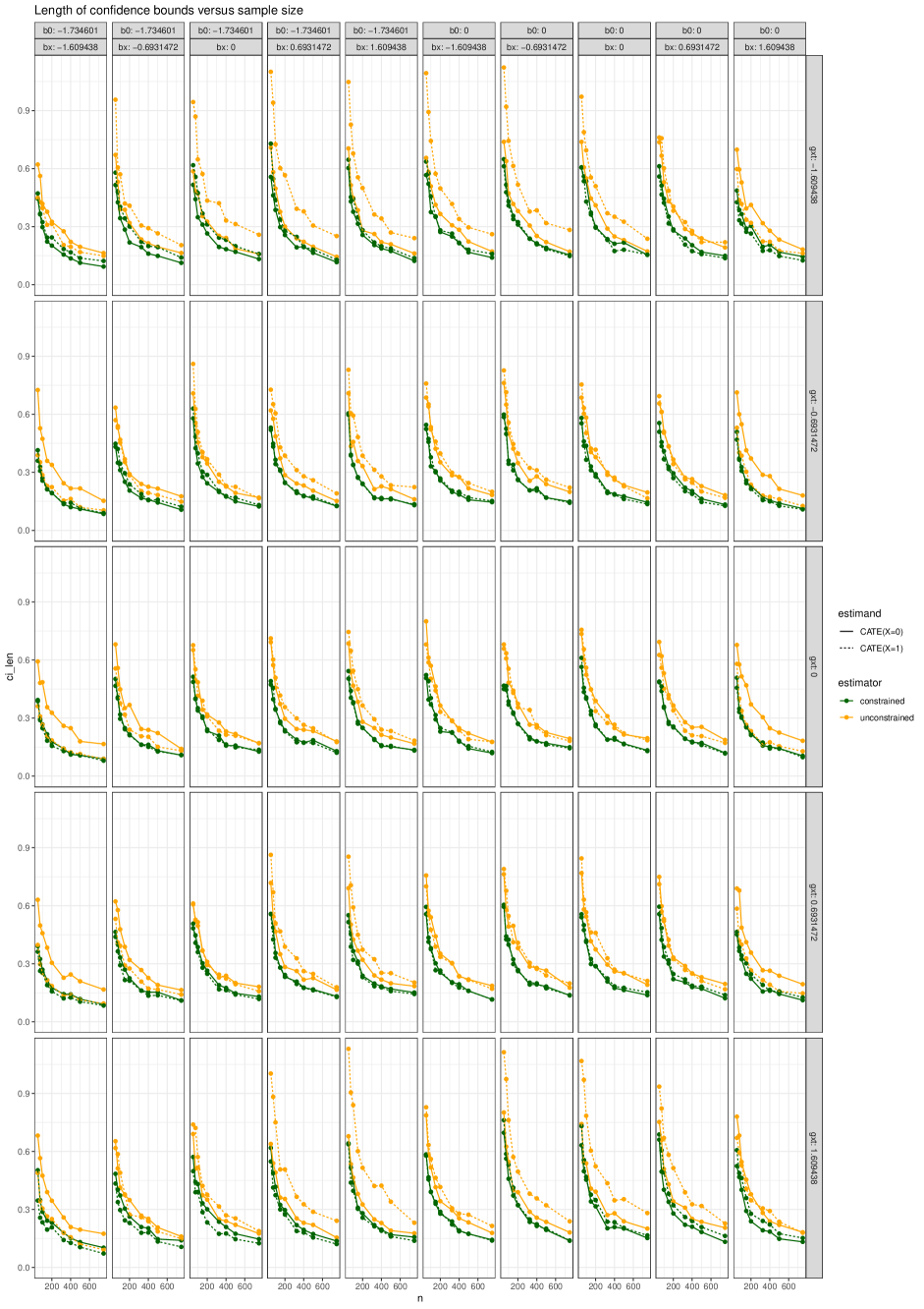
Figure 4:

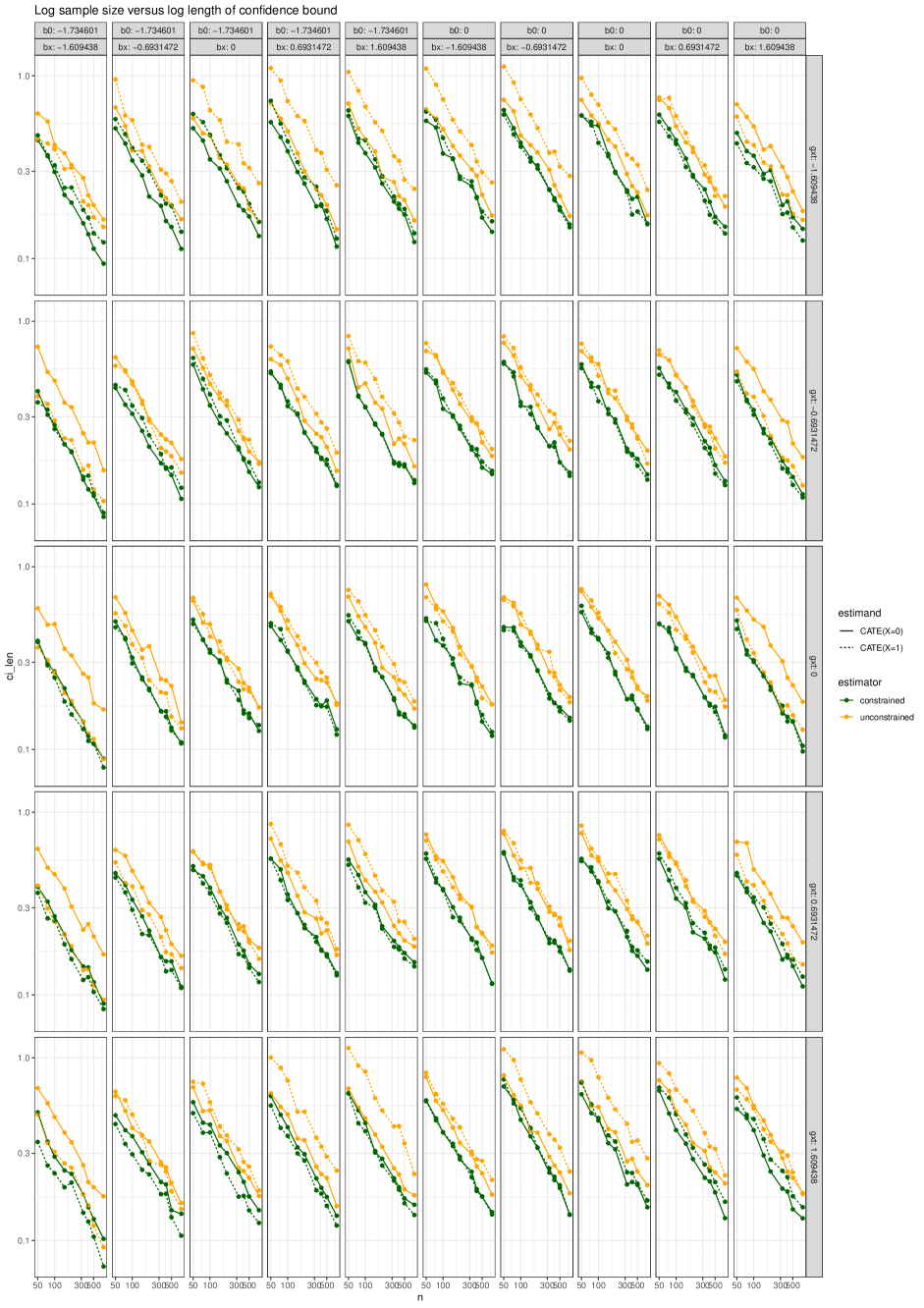
Figure 5:

References

• [1] Murray EJ, Caniglia EC, Swanson SA, HernΓ‘ndez-DΓ­az S, HernΓ‘n MA. Patients and investigators prefer measures of absolute risk in subgroups for pragmatic randomized trials. Journal of Clinical Epidemiology. 2018 Nov;103:10–21.
• [2] Causal Diagrams and the Identification of Causal Effects. In: Pearl J, editor. Causality. Cambridge: Cambridge University Press; 2009. p. 65–106. Available from: https://www.cambridge.org/core/books/causality/causal-diagrams-and-the-identification-of-causal-effects/D9AE074727C3AC9AFE9F0CD4C7A506B5.
• [3] Furie R, Rovin BH, Houssiau F, Malvar A, Teng YKO, Contreras G, etΒ al. Two-Year, Randomized, Controlled Trial of Belimumab in Lupus Nephritis. The New England Journal of Medicine. 2020 Sep;383(12):1117–1128.
• [4] Lean ME, Leslie WS, Barnes AC, Brosnahan N, Thom G, McCombie L, etΒ al. Primary care-led weight management for remission of type 2 diabetes (DiRECT): an open-label, cluster-randomised trial. Lancet (London, England). 2018 Feb;391(10120):541–551.
• [5] CandidoΒ dos Reis FJ, Wishart GC, Dicks EM, Greenberg D, Rashbass J, Schmidt MK, etΒ al. An updated PREDICT breast cancer prognostication and treatment benefit prediction model with independent validation. Breast Cancer Research. 2017 Dec;19(1):58. 80 citations (Crossref) [2021-08-06]. Available from: http://breast-cancer-research.biomedcentral.com/articles/10.1186/s13058-017-0852-3.
• [6] Ravdin PM, Siminoff LA, Davis GJ, Mercer MB, Hewlett J, Gerson N, etΒ al. Computer Program to Assist in Making Decisions About Adjuvant Therapy for Women With Early Breast Cancer. Journal of Clinical Oncology. 2001 Feb;19(4):980–991. 679 citations (Crossref) [2021-08-06]. Available from: http://ascopubs.org/doi/10.1200/JCO.2001.19.4.980.
• [7] Alaa AM, Gurdasani D, Harris AL, Rashbass J, vanΒ der Schaar M. Machine learning to guide the use of adjuvant therapies for breast cancer. Nature Machine Intelligence. 2021 Aug;3(8):716–726. Bandiera_abtest: a Cg_type: Nature Research Journals Number: 8 Primary_atype: Research Publisher: Nature Publishing Group Subject_term: Breast cancer;Prognosis Subject_term_id: breast-cancer;prognosis. Available from: https://www.nature.com/articles/s42256-021-00353-8.
• [8] Xu Z, Arnold M, Stevens D, Kaptoge S, Pennells L, Sweeting MJ, etΒ al. Prediction of Cardiovascular Disease Risk Accounting for Future Initiation of Statin Treatment. American Journal of Epidemiology. 2021 Feb:kwab031. Available from: https://academic.oup.com/aje/advance-article/doi/10.1093/aje/kwab031/6140872.
• [9] Cardoso F, Kyriakides S, Ohno S, Penault-Llorca F, Poortmans P, Rubio IT, etΒ al. Early breast cancer: ESMO Clinical Practice Guidelines for diagnosis, treatment and follow-up. Annals of Oncology. 2019 Aug;30(8):1194–1220. Available from: https://linkinghub.elsevier.com/retrieve/pii/S0923753419312876.
• [10] Gradishar WJ. NCCN Breast Cancer Guideline, Version 5.2021; 2021. Available from: https://www.nccn.org/professionals/physician_gls/pdf/breast-2.pdf.
• [11] Hill JL. Bayesian Nonparametric Modeling for Causal Inference. Journal of Computational and Graphical Statistics. 2011 Jan;20(1):217–240. Available from: http://www.tandfonline.com/doi/abs/10.1198/jcgs.2010.08162.
• [12] Suverein MM, Delnoij TSR, Lorusso R, Brandon BravoΒ Bruinsma GJ, Otterspoor L, ElzoΒ Kraemer CV, etΒ al. Early Extracorporeal CPR for Refractory Out-of-Hospital Cardiac Arrest. New England Journal of Medicine. 2023 Jan;388(4):299–309. Available from: http://www.nejm.org/doi/10.1056/NEJMoa2204511.
• [13] Hill KD, Kannankeril PJ, Jacobs JP, Baldwin HS, Jacobs ML, O’Brien SM, etΒ al. Methylprednisolone for Heart Surgery in Infants β€” A Randomized, Controlled Trial. New England Journal of Medicine. 2022 Dec;387(23):2138–2149. Available from: http://www.nejm.org/doi/10.1056/NEJMoa2212667.
• [14] Weghuber D, Barrett T, Barrientos-PΓ©rez M, Gies I, Hesse D, Jeppesen OK, etΒ al. Once-Weekly Semaglutide in Adolescents with Obesity. New England Journal of Medicine. 2022 Dec;387(24):2245–2257. Available from: http://www.nejm.org/doi/10.1056/NEJMoa2208601.
• [15] TchetgenΒ Tchetgen EJ, Robins JM, Rotnitzky A. On doubly robust estimation in a semiparametric odds ratio model. Biometrika. 2010 Mar;97(1):171–180. Available from: https://www.ncbi.nlm.nih.gov/pmc/articles/PMC3412601/.
• [16] TchetgenΒ Tchetgen EJ, Rotnitzky A. Double-robust estimation of an exposure-outcome odds ratio adjusting for confounding in cohort and case-control studies. Statistics in Medicine. 2011 Feb;30(4):335–347.
• [17] Watson T. Practitioner’s Guide to Generalized Linear Models. Towers Watson; 2007.
• [18] Engels EA, Schmid CH, Terrin N, Olkin I, Lau J. Heterogeneity and statistical significance in meta-analysis: an empirical study of 125 meta-analyses. Statistics in Medicine. 2000 Jul;19(13):1707–1728.
• [19] Huitfeldt A, Stensrud MJ, Suzuki E. On the collapsibility of measures of effect in the counterfactual causal framework. Emerging Themes in Epidemiology. 2019 Jan;16(1):1. Available from: https://doi.org/10.1186/s12982-018-0083-9.
• [20] Didelez V, Stensrud MJ. On the logic of collapsibility for causal effect measures. Biometrical Journal. 2022;64(2):235–242. _eprint: https://onlinelibrary.wiley.com/doi/pdf/10.1002/bimj.202000305. Available from: https://onlinelibrary.wiley.com/doi/abs/10.1002/bimj.202000305.
• [21] Whittemore AS. Collapsibility of Multidimensional Contingency Tables. Journal of the Royal Statistical Society Series B (Methodological). 1978;40(3):328–340. Publisher: [Royal Statistical Society, Wiley]. Available from: https://www.jstor.org/stable/2984697.
• [22] Daniel R, Zhang J, Farewell D. Making apples from oranges: Comparing noncollapsible effect estimators and their standard errors after adjustment for different covariate sets. Biometrical Journal. 2021;63(3):528–557. _eprint: https://onlinelibrary.wiley.com/doi/pdf/10.1002/bimj.201900297. Available from: https://onlinelibrary.wiley.com/doi/abs/10.1002/bimj.201900297.
• [23] Hauck WW, Neuhaus JM, Kalbfleisch JD, Anderson S. A consequence of omitted covariates when estimating odds ratios. Journal of Clinical Epidemiology. 1991 Jan;44(1):77–81. Available from: https://www.sciencedirect.com/science/article/pii/089543569190203L.
• [24] Pearl J. Causal inference in statistics: An overview. Statistics Surveys. 2009 Jan;3(none). Available from: https://projecteuclid.org/journals/statistics-surveys/volume-3/issue-none/Causal-inference-in-statistics-An-overview/10.1214/09-SS057.full.
• [25] Hernan MA, Robins JM. Causal Inference: What If. 2020.
• [26] Wald A. The Fitting of Straight Lines if Both Variables are Subject to Error. The Annals of Mathematical Statistics. 1940 Sep;11(3):284–300. Publisher: Institute of Mathematical Statistics. Available from: https://projecteuclid.org/journals/annals-of-mathematical-statistics/volume-11/issue-3/The-Fitting-of-Straight-Lines-if-Both-Variables-are-Subject/10.1214/aoms/1177731868.full.
• [27] Hartford J, Lewis G, Leyton-Brown K, Taddy M. Deep IV: A flexible approach for counterfactual prediction. In: International Conference on Machine Learning. PMLR; 2017. p. 1414–1423.
• [28] Puli A, Ranganath R. General Control Functions for Causal Effect Estimation from IVs. Advances in neural information processing systems. 2020;33:8440–8451.
• [29] Miao W, Geng Z, TchetgenΒ Tchetgen EJ. Identifying causal effects with proxy variables of an unmeasured confounder. Biometrika. 2018 Dec;105(4):987–993. Available from: https://doi.org/10.1093/biomet/asy038.
• [30] van Amsterdam WAC, Verhoeff JJC, Harlianto NI, Bartholomeus GA, Puli AM, deΒ Jong PA, etΒ al. Individual treatment effect estimation in the presence of unobserved confounding using proxies: a cohort study in stage III non-small cell lung cancer. Scientific Reports. 2022 Apr;12(1):5848. Number: 1 Publisher: Nature Publishing Group. Available from: https://www.nature.com/articles/s41598-022-09775-9.
• [31] Ilse M, ForrΓ© P, Welling M, Mooij JM. Combining Interventional and Observational Data Using Causal Reductions. arXiv:210304786 [cs, stat]. 2022 Jan. ArXiv: 2103.04786. Available from: http://arxiv.org/abs/2103.04786.
• [32] Bradbury J, Frostig R, Hawkins P, Johnson MJ, Leary C, Maclaurin D, etΒ al.. JAX: composable transformations of Python+NumPy programs; 2018. Available from: http://github.com/google/jax.
• [33] Blondel M, Berthet Q, Cuturi M, Frostig R, Hoyer S, Llinares-LΓ³pez F, etΒ al.. Efficient and Modular Implicit Differentiation. arXiv; 2022. ArXiv:2105.15183 [cs, math, stat]. Available from: http://arxiv.org/abs/2105.15183.
• [34] Phan D, Pradhan N, Jankowiak M. Composable Effects for Flexible and Accelerated Probabilistic Programming in NumPyro. arXiv preprint arXiv:191211554. 2019.
• [35] Group EBCTC. Tamoxifen for early breast cancer: an overview of the randomised trials. The Lancet. 1998 May;351(9114):1451–1467. Available from: https://www.sciencedirect.com/science/article/pii/S0140673697114234.
• [36] Rosenman E, Basse G, Owen A, Baiocchi M. Combining Observational and Experimental Datasets Using Shrinkage Estimators. arXiv:200206708 [math, stat]. 2020 May. ArXiv: 2002.06708. Available from: http://arxiv.org/abs/2002.06708.