Participatory Sensing for Localization of a GNSS Jammer

Abstract

GNSS receivers are vulnerable to jamming and spoofing attacks, and numerous such incidents have been reported worldwide in the last decade. It is important to detect attacks fast and localize attackers, which can be hard if not impossible without dedicated sensing infrastructure. The notion of participatory sensing, or crowdsensing, is that a large ensemble of voluntary contributors provides the measurements, rather than relying on dedicated sensing infrastructure. This work considers embedded GNSS receivers to provide measurements for participatory jamming detection and localization. Specifically, this work proposes a novel jamming localization algorithm, based on participatory sensing, that exploits AGC and $C/N_{0}$ estimates from commercial GNSS receivers. The proposed algorithm does not require knowledge of the jamming power nor of the channels, but automatically estimates all parameters. The algorithm is shown to outperform similar state-of-the-art localization algorithms in relevant scenarios.

I Introduction

Global Navigation Satellite System (GNSS) receivers are widely spread in numerous society-critical services today. At the same time, GNSS receivers are vulnerable to jamming and spoofing attacks, and numerous GNSS jamming and spoofing incidents have been reported worldwide in the last decade. Detecting, and more importantly, localizing the source of such attacks is therefore of significant importance.

Considering that any GNSS equipped device could be targeted by an attack, measurements available at GNSS receivers can be the basis for the detection and localization of an attack at each device. Typically, GNSS receivers are embedded in a wide gamut of networked devices (e.g., smart-phones, vehicles). This enables each affected device to share data of such an event with other devices, typically with the help of a data aggregating service. This is the notion of participatory sensing, or crowdsensing: rather than relying on dedicated sensing infrastructure, a large ensemble of voluntary contributors provides the necessary measurements. In our scenario, the sensors are GNSS receivers embedded in a conncected device and measurements refer to the data available in such GNSS receivers. GNSS receivers offer a rich interface to radio measurements that can be valuable in detecting attacks and localizing attacking devices. This motivated a number of recent publications that deal with detection or localization of GNSS interference using a crowdsensing approach (cf. [1, 2, 3, 4, 5]). These works are based on some sort of power measurement, usually through carrier-to-noise-density ratio ($C/N_{0}$) estimates or automatic gain control (AGC) values, but in some cases through direct power measurements. $C/N_{0}$ measurements, and sometimes AGC, are provided by all grades of GNSS receivers, from low-cost to professional, which allows jammer localization using different types of commercial sensors.

[1, 2, 3, 4] utilizes the $C/N_{0}$ and a simple distance dependent path loss model, and computes the jammer position based on a least squares (LS) solution for multiple receivers. The LS localization algorithm of [1] is derived for a single moving receiver which can be viewed as a synthetic array. An algorithm for multiple receivers, that takes the average location of those receivers that detect the jammer, is also proposed in [1]. This algorithm is further extended in [5] to obtain a weighted average solution, rather than just a plain average.

There are other related papers that deal with power difference of arrival (PDOA) algorithms [6]. These are similar to exploiting AGC or $C/N_{0}$ measurements, but they are assumed to measure, or estimate, the received power directly. Some of these even assume that the power difference is estimated from the AGC [6, 7].

The model assumptions of [1, 2, 3, 5, 4, 6, 7] are very similar to those used in this work. The main differences are that our work extends the models of [1, 2, 3, 5, 4, 6, 7] by assuming an unknown channel (i.e., the path loss exponent) between the receivers and jammer and a random measurement error is included. This is necessary for practical application. The work of [7] also deals with an unknown path loss exponent using time difference of arrival (TDOA). That approach, however, requires access to baseband I/Q data which are not available in a standard embedded GNSS receiver and is therefore not a suitable algorithm for a participatory sensing scenario. In addition, our proposed algorithm does not require pre-calibration of the sensing receivers with respect to the jamming power, contrary to the algorithms of [1, 2, 3, 5].

Mobile phone based crowdsourcing for jamming detection and localization is considered in [8, 9]. The basic concept of using AGC or $C/N_{0}$ measurements from mobile phones for localization purposes is proposed in [8], and field trials show the usefulness of these metrics. However, no explicit localization algorithm is proposed in [8]. [9] proposes a localization algorithm based on $C/N_{0}$ measurements in combination with step detection and step length estimation using an inertial sensor. The algorithm of [9] assumes a sensor that moves along a straight line in two perpendicular directions, which is highly limiting in a participatory sensing system.

The main contribution of this work is a novel jamming localization algorithm, based on participatory sensing, that

• does not need any pre-calibration or channel knowledge but automatically estimates all parameters,

• exploits AGC or $C/N_{0}$ estimates, or a combination thereof, from commercial GNSS receivers,

• outperforms existing similar algorithms in relevant scenarios.

II System Model

We do not dwell in this paper on the networking specifics or the security and privacy of the collected data (e.g., [10, 11]). Rather, we assume ${N_{\text{r}}}$ receivers measure AGC and $C/N_{0}$ and submit those to a central server, where the localization algorithm is run. Measurements are submitted at a specified common rate, typically in the order of 1 Hz from a standard mobile phone. Submitted data are assumed to be either time-stamped or can be otherwise synchronized at an accuracy within the common time epoch of each measurement.

The proposed algorithm is based on the following assumptions:

• the receivers have isotropic antennas,

• the jammer has an isotropic antenna,

• the jammer position, denoted by ${\mathbf{p}}_{0}=[x_{0},y_{0},z_{0}]^{T}$, is fixed during the time of mesurement,

• the jamming power, denoted by $J_{0}$, is constant during the time of mesurement,

• receiver noise powers are constant during the time of mesurement,

• the receiver positions, denoted by ${\mathbf{p}}_{i}[n]=[x_{i}[n],y_{i}[n],z_{i}[n]]^{T}$ at time $n$ for receiver $i=1,\ldots,{N_{\text{r}}}$, are known.

These assumptions are also made (explicitly or implicitly) in [1, 2, 3, 5]. It should be noted that the assumptions should be valid only within each measurement time frame, which is a design parameter. The assumption of isotropic antennas boils down to an assumption of the channel gains being constant during the time of measurement, which is required for estimating the channel. Constant noise powers within each measurement time frame is a fair approximation for the relatively short measurement times that are of interest. Constant jamming power is valid for most commercial jammers. The receiver positions can be assumed known by integration of GNSS and other sensors, such as an inertial measurement unit (IMU), embedded in the sensor device (e.g. a cell phone). That is, at any point in time the sensing device has a current own position estimate it uses to geostamp the contributed measurement. It should be noted that the proposed algorithm estimates a jammer position even if these assumptions do not hold perfectly, but of course the estimation error becomes larger if, for example, the jammer moves during the observation time.

The goal is to estimate the position ${\mathbf{p}}_{0}$ of the jammer. The model for AGC measurements is explained first, followed by an analogous model for $C/N_{0}$ estimates.

II-A AGC

Let $h_{i}[n]$ denote the channel (power) gain between the attacker and receiver $i$ at time $n$. The channel gain $h_{i}[n]$ depends on the distance $d_{i}[n]\triangleq\left\lVert{{\mathbf{p}}_{0}-{\mathbf{p}}_{i}[n]}\right\rVert=\sqrt{(x_{0}-x_{i}[n])^{2}+(y_{0}-y_{i}[n])^{2}+(z_{0}-z_{i}[n])^{2}}$). Then, the received jamming power $J_{i}[n]$ is

$$J_{i}[n]=J_{0}h_{i}[n].$$

A path loss model where $h_{i}[n]\propto 1/d_{i}[n]^{\alpha_{i}}$ yields

$$J_{i}[n]=\frac{J_{0}\kappa}{d_{i}[n]^{\alpha_{i}}},$$

where $\alpha_{i}$ is the path loss exponent for receiver $i$ and $\kappa$ is a proportionality constant. The constant $\kappa$ depends on, for example, carrier frequency and antenna gain, which are constant and equal for all receivers as all antennas are assumed to be isotropic. The path loss exponents $\alpha_{i}$ are assumed to be unknown in this work and are estimated as explained in Section III.

The total received power, denoted by $P_{i}[n]$, can be written

$$P_{i}[n]=J_{i}[n]+N_{G,i}+\sum_{j=1}^{{N_{\text{m}}}}C_{i,j}[n],$$

where $N_{G,i}$ is the background noise power at the input to the AGC circuit of receiver $i$, assumed to be constant during the time of measurement, and $C_{i,j}[n]$ denotes the power of the visible satellite signal $j=1,\ldots,{N_{\text{m}}}$ at receiver $i$. The received powers of the satellite signals (before despreading) are small compared to the receiver noise power and can therefore be neglected, i.e.,

$$P_{i}[n]\approx J_{i}[n]+N_{G,i}=\frac{J_{0}\kappa}{d_{i}[n]^{\alpha_{i}}}+N_{G,i}.$$

Let $g_{i}[n]$ be the AGC value for receiver $i=1,\ldots,{N_{\text{r}}}$ at time $n$. Then, ideally, ([12, 13])

$$g_{i}[n]\sqrt{P_{i}[n]}=\sqrt{\bar{P}_{i}},$$

where $\sqrt{\bar{P}_{i}}$ is the desired received signal amplitude. The AGC gain in the absence of jamming ($J_{0}=0$), denoted by $\bar{g}_{i}$, is assumed to be known and can be written

$$\bar{g}_{i}\sqrt{N_{G,i}}=\sqrt{\bar{P}_{i}}.$$

In practice, $\bar{g}_{i}$ can easily be estimated at initialization or by long-term estimation. It should be noted that the algorithm uses the difference relative to the non-jammed AGC value, $\bar{g}_{i}$, and not the absolute measurement. This is important, because the absolute AGC estimates may vary significantly across devices [14]. Then,

$$g_{i}[n]=\frac{\sqrt{\bar{P}_{i}}}{\sqrt{P_{i}[n]}}=\bar{g}_{i}\sqrt{\frac{N_{G,i}}{P_{i}[n]}}=\bar{g}_{i}\sqrt{\frac{N_{G,i}}{\frac{J_{0}\kappa}{d_{i}[n]^{\alpha_{i}}}+N_{G,i}}}.$$

Let $G_{i}[n]$ and $\bar{G}_{i}$ denote $g_{i}[n]$ and $\bar{g}_{i}$, respectively, in decibels. That is, $G_{i}[n]\triangleq 20\mathrm{log}_{10}(g_{i}[n])$ and $\bar{G}_{i}\triangleq 20\mathrm{log}_{10}(\bar{g}_{i})$. Then, the measurement model, with additional measurement noise, can be written as

$$G_{i}[n]=\bar{G}_{i}-10\mathrm{log}_{10}\left(\frac{J_{0}\kappa}{N_{G,i}}d_{i}[n]^{-\alpha_{i}}+1\right)+w_{G_{i}}[n],$$ (1)

where $w_{G_{i}}[n]\sim\mathcal{N}(0,\,\sigma_{G,i}^{2})$ denotes measurement noise.

II-B $C/N_{0}$

Let $s_{i,j}[n]$ denote the observed carrier-to-noise-and-interference ratio (CNIR), which is estimated by the GNSS receivers and commonly, with slight abuse of terminology, referred to as $C/N_{0}$. Let $N_{0,i}$ denote the background noise power spectral density at receiver $i$, and $\tilde{J}_{i}[n]$ a spectrally-flat-equivalent interference noise power density [15] at receiver $i$. Then, the CNIR can be written as

$$s_{i,j}[n]\triangleq\frac{C_{i,j}[n]}{N_{0,i}+\tilde{J}_{i}[n]}=\frac{C_{i,j}[n]}{N_{0,i}}\cdot\frac{1}{1+\frac{\tilde{J}_{i}[n]}{N_{0,i}}}.$$

Multiplying $\tilde{J}_{i}[n]$ and $N_{0,i}$ in the denominator with the receiver bandwidth, thereby cancelling the bandwidth dependence, and taking the mean CNIR values from all received satellite signals yields

$$s_{i}[n]=\frac{1}{N_{m}}\sum_{j=1}^{N_{m}}\left(\frac{C_{i,j}[n]}{N_{0,i}}\cdot\frac{1}{1+\frac{J_{i}[n]}{N_{S,i}}}\right),$$

where $N_{S,i}$ is the noise power experienced in CNIR estimation. Note that the noise power at the CNIR estimator, $N_{S,i}$, is not in general equal to the AGC input noise, $N_{G,i}$. $N_{S,i}$ includes additional noise from circuits (such as low-noise amplifiers) inbetween the AGC and the CNIR estimator. Moreover, it is estimated in the post-correlation step, whereas the $N_{G,i}$ noise is experienced on the pre-correlation input signal.

Let $\bar{s}_{i}$ be the mean CNIR with no jamming ($J_{i}[n]=0$), which is assumed to be known. In practice, $\bar{s}_{i}$ can easily be estimated at startup (assuming there is no jamming) or by long-term estimation of the measured CNIR. That is

$$\bar{s}_{i}=\frac{1}{N_{m}}\sum_{j=1}^{N_{m}}\frac{C_{i,j}[n]}{N_{0,i}}.$$

Recall that the jammer localization algorithm uses the difference relative to the non-jammed value $\bar{s}_{i}$ and not the measurement itself in absolute numbers, to avoid significant variations across devices. Then,

$$s_{i}[n]=\bar{s}_{i}\cdot\frac{1}{1+\frac{J_{i}[n]}{N_{S,i}}}.$$

By switching to logarithmic scale, i.e. using $S_{i}[n]$ and $\bar{S}_{i}$ to denote $s_{i}$ and $\bar{s}_{i}$, respectively, in decibels, the measurement model is written as

$$S_{i}[n]=\bar{S}_{i}-10\mathrm{log}_{10}\left(\frac{J_{0}\kappa}{N_{S,i}}d_{i}^{-\alpha_{i}}[n]+1\right)+w_{S_{i}}[n],$$ (2)

where $w_{S_{i}}[n]\sim\mathcal{N}(0,\,\sigma_{S_{i}}^{2})\,$, which is analogous to (1). From here on, only the AGC measurement model will be used, but the CNIR measurement model can be used in the same way since equations (1) and (2) are identical.

III Jammer Position Estimation

We derive an algorithm that estimates the unknown jammer position ${\mathbf{p}}_{0}$. In addition to ${\mathbf{p}}_{0}$, there are several unknown nuisance parameters that need to be taken into account. To simplify notation, the model is parametrized as follows:

$$\zeta_{i}\triangleq\frac{J_{0}\kappa}{N_{G,i}},\ \ {\boldsymbol{\zeta}}\triangleq[\zeta_{1},\ldots,\zeta_{N_{\text{r}}}]^{T},$$

$${\boldsymbol{\alpha}}\triangleq[\alpha_{1},\ldots,\alpha_{N_{\text{r}}}],\ \ {\boldsymbol{\sigma}}_{G}^{2}\triangleq[\sigma_{G,1}^{2},\ldots,\sigma_{G,{N_{\text{r}}}}^{2}].$$

III-A Joint Estimation

To perform joint estimation of the position based on all jammed sensors, ${N_{\text{r}}}$, the AGC observations for time instances $n=1,\ldots,N$ are combined in the matrix

$${\mathbf{G}}\triangleq\begin{bmatrix}G_{1}[1]&G_{2}[1]&\ldots&G_{N_{\text{r}}}[1]\\ G_{1}[2]&G_{2}[2]&\ldots&G_{N_{\text{r}}}[2]\\ \vdots&\vdots&\ddots&\vdots\\ G_{1}[N]&G_{2}[N]&\ldots&G_{N_{\text{r}}}[N]\\ \end{bmatrix},$$

and the known AGC levels in the absence of jamming in the vector

$$\bar{\mathbf{G}}\triangleq\begin{bmatrix}\bar{G}_{1}&\bar{G}_{2}&\ldots&\bar{G}_{N_{\text{r}}}\end{bmatrix}.$$

The likelihood function for the AGC measurements is then

$$\begin{split}&p({\mathbf{G}}|\bar{\mathbf{G}},{\mathbf{p}}_{0},{\boldsymbol{\alpha}},{\boldsymbol{\zeta}},{\boldsymbol{\sigma}}_{G}^{2})=\\ &=\prod_{i=1}^{N_{\text{r}}}(2\pi\sigma_{G,i}^{2})^{-N/2}\mathrm{exp}\Big{[}-\frac{1}{2\sigma_{G,i}^{2}}\sum_{n=1}^{N}(G_{i}[n]-\\ &(\bar{G}_{i}-10\mathrm{log}_{10}(\zeta_{i}d_{i}^{-\alpha_{i}}[n]+1)))^{2}\Big{]}.\end{split}$$ (3)

The jammer position is found by maximizing the likelihood function as

$${\mathbf{p}}_{0}^{*}=\underset{{\mathbf{p}}_{0},{\boldsymbol{\zeta}},{\boldsymbol{\sigma}}_{G}^{2},{\boldsymbol{\alpha}}}{\operatorname{argmax}\ }p({\mathbf{G}}|\bar{\mathbf{G}},{\mathbf{p}}_{0},{\boldsymbol{\alpha}},{\boldsymbol{\zeta}},{\boldsymbol{\sigma}}_{G}^{2}).$$ (4)

III-B Estimation from a Subset of Sensors

The joint estimation may not perform well if some of the sensors are unreliable or do not fit the model well. This occurs, for example, if the channel model $h_{i}[n]\propto 1/d_{i}[n]^{\alpha_{i}}$ is inaccurate for some sensors, especially if the jamming signal is obstructed. Many other algorithms, such as [2, 1], assume that $\alpha_{i}=2$ which is true in ideal free space propagation. In practical cases, the path loss may differ from 2 and hence cause, eventually, significant sensor-jammer distance estimation errors. Therefore, the final position estimate is based on the subset of the available sensors deemed to be more accurate, thus more useful. Receivers that have free sight to the jammer and hence $\alpha_{i}\approx 2$ are most useful in terms of accurately estimating the distance to the jammer. Therefore, in this work, receivers with estimated $\alpha_{i}\leq 2.3$ are deemed useful for the localization estiamation.

To select the desired set of most useful sensors, the path loss exponent $\alpha_{i}$ is estimated for each sensor individually by maximizing the likelihood function using that particular receiver only, and different values of $\alpha_{i}$ using a grid search. The value of $\alpha_{i}$ that results in the highest likelihood is then chosen as the path loss exponent estimate for that receiver. The joint position estimate is then calculated by maximizing the likelihood function, using only the most useful receivers with their estimated pathloss exponents.

III-C Maximizing the Likelihood Function

The maximization (4) cannot be solved analytically, but must be solved using numerical methods. The likelihood function is maximized using gradient descent on the negative log-likelihood. The parameter ${\boldsymbol{\sigma}}_{G}$ can, however, be solved analytically, conditioned on the other unkown parameters, as

$$\sigma_{G,i}^{2}=\frac{1}{N}\sum_{n=1}^{N}(G_{i}[n]-\bar{G}_{i}+10\log_{10}(\zeta_{i}d_{i}^{-\alpha_{i}}[n]+1))^{2}$$

when using AGC.

Hence, the ${\boldsymbol{\sigma}}_{G}$ is computed according to this expression after each iteration of the gradient descent.

The initial jammer position estimate is set to the mean start position of the receivers, i.e., ${\mathbf{p}}_{0}=\frac{1}{{N_{\text{r}}}}\sum_{i=1}^{{N_{\text{r}}}}{\mathbf{p}}_{i}[0]$, and ${\boldsymbol{\sigma}}_{G}^{2}$ is initiated to the variance of the AGC value of each receiver when no jamming is present. During the pathloss exponent estimation, ${\boldsymbol{\zeta}}$ is initialized to ${10}^{8}\text{\,}$. The resultant ${\boldsymbol{\zeta}}$ values after the path loss estimation gradient descent are used as initial values during the joint estimation.

In order to find a suitable stepsize during the descent, the backtracking line search is utilized, first proposed in [16]. The path loss exponent, ${\boldsymbol{\alpha}}$, is optimized through grid search and is not a part of the gradient descent. That is, ${\boldsymbol{\alpha}}$ is chosen beforehand from a grid and then held fixed during the gradient descent computation. The reason for this is that the gradient descent does not converge well to the correct value of ${\boldsymbol{\alpha}}$ in general.

IV Numerical Results

The proposed algorithm is evaluated numerically, and compared to state-of-the-art methods. Monte Carlo simulations are used to evaluate the performance of the algorithms. For each Monte Carlo-run, the start positions of the receivers are placed at a uniformly random point within a cube with a side length of 2000 meters, with the jammer placed at the center of the cube. The jammer transmits a signal with power $0.01\text{\,}\mathrm{W}$ over the same bandwidth used by the victim receivers.

The scenario starts at a random time of day and goes on for a predefined length of time. The receivers are mobile, travelling from their start point in a random direction with a preset constant speed and the jammer is activated halfway through the scenario. The samples from the first half of the scenario, where no jamming is present, is used to estimate $\bar{G}_{i}$. The samples from the second half of the scenario is used as the AGC observations, ${\mathbf{G}}$, in the likelihood function (4). If a measurement from a receiver drops down -5dB from $\bar{G}_{i}$ at any time during the scenario, the receiver is considered to be jammed and it is used in the joint estimation. The path loss exponent between each receiver and the jammer is set to 2, with an added random error taken from a half-normal distribution with scale parameter $0.1$.

In Sections IV-A to IV-C, the AGC model (3) is used and compared to the algorithms presented in [2, 1], for GNSS jamming localization based on crowdsourced measurements, that is, the state-of-the-art. Both algorithms are based on similar properties as the algorithm proposed in this work. The main difference between the two compared algorithms and this work is that the proposed novel algorithm also considers measurement noise and unknown path loss exponents, which is necessary for practical application. To do a fair comparison, the compared algorithms are modified to use AGC measurements in lieu of CNIR. The algorithm of [1] estimates the jammer position as the mean of the positions of all detecting receivers. The algorithm of [2] is based on a least-squares estimate. For the method in [2], the receivers are calibrated with a known jamming power observed at a known distance and the path loss exponents are assumed to be $\alpha_{i}=2$, even when the actual path loss differs from $2$ in the simulations.

IV-A Different Number of Receivers

The performance dependence on the number of receivers is evaluated in this section. Ten scenarios, each with a different number of receivers, are tested, from 3 to 30 receivers. Two different mobility scenarios are evaluated, and results are shown in Figures 1 and 2 respectively. In the first scenario, the receivers’ starting positions are placed uniformly inside a cube. In the second scenario, all receivers are traveling along a straight line going in a north-south direction 500 meters east of the jammer. The measurement noise variance is set to $\sigma_{G,i}^{2}=0.1$, and the speed of the receivers is $1.5\text{\,}\mathrm{m}\mathrm{/}\mathrm{s}$. The total time of the scenario is 3000 seconds, with a total of $N=200$ observation samples per receiver. A total of 1000 Monte Carlo simulations are made.

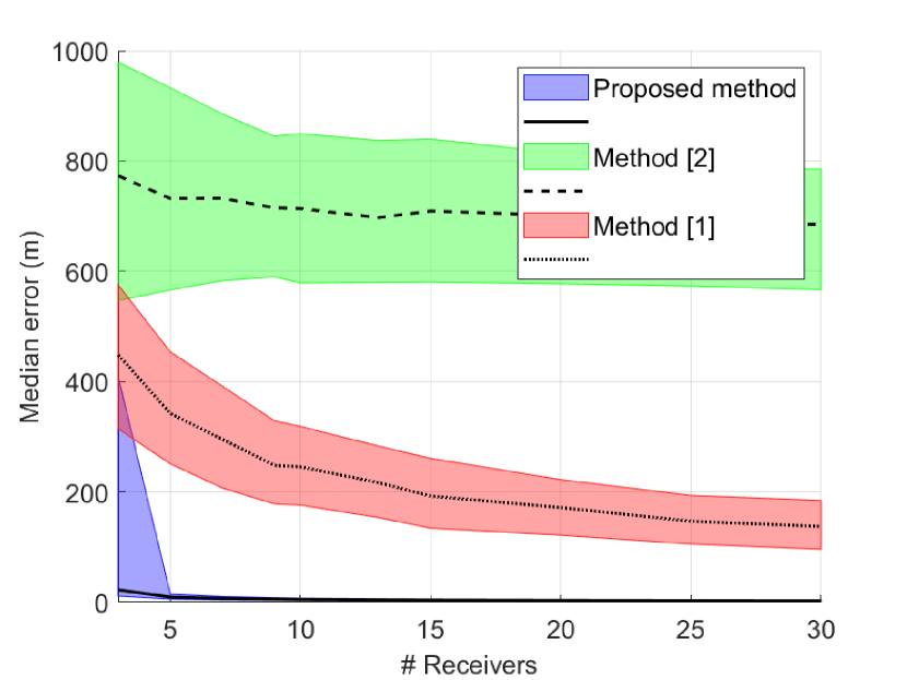
Figure 1: Median 3D-error (black lines) and 25th to 75th percentile (shaded areas) for the three different methods using different number of receivers.

The results can be seen in Figure 1, which shows the median estimation error as a function of the number of receivers. It can be seen that the proposed algorithm using AGC achieves smaller localization error than the state-of-the-art algorithms we compare to. For example, the proposed algorithm achieves a median 3D-error of less than 5 meters when using AGC mesurements in the simulated scenario with 10 receivers. The corresponding errors are 698 meters and 217 meters when using method [2] and [1].

What also can be seen from Figure 1 is that the error decreases quickly with the number of receivers. Going from 3 to 5 receivers decreases the 75th percentile of the 3D-error from 400 meters to 15 meters when using AGC. Such big decreases are not seen in the compared methods, which gives our method an advantage in the sense that it would not require as many receivers to get a good estimate.

While the error of method [1] decreases with increasing number of receivers, this might be a bit misleading. In this testcase, the receivers are placed using a uniform distribution over the area surrounding the jammer, and with added receivers the centroid moves towards the origin, where the jammer is placed. If the jammer is placed somewhere else, the result would be worse. This problem is observed in a scenario where all receivers are traveling along a straight line going in a north-south direction, 500 meters east of the jammer. All receivers are placed at the same height as the transmitter.

The result is shown in Figure 2. The error shown is the two-dimensional error, not taking the elevation in consideration, since the receivers have the same elevation as the transmitter in this scenario. The error never gets smaller than 500 meters for algorithm [1], while the proposed method achieves a smaller error in a majority of the simulations, even though it is not as accurate as when the receivers are placed uniformly. The loss in accuracy comes from the fact that all receivers are located on the same side of the jammer, and hence the receiver geometry is worse than if they are spread around the jammer.

The algorithm [2] has a hard time finding a solution to the least squares problem during the road scenario, not giving a solution at all for 68% of the simulations for 30 receivers and 99% of the simulations for 3 receivers, and is therefore not shown in Figure 2.

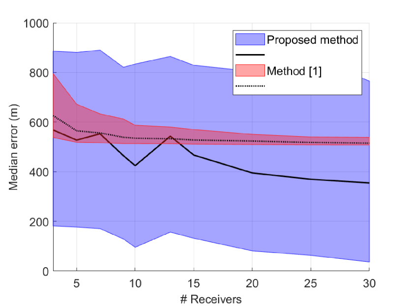
Figure 2: Median 2D-error (black lines) and 25th to 75th percentile (shaded areas) for the proposed method and method [1], using different number of receivers. Receivers travel along a straight line, 500 meters east of the origin.

IV-B Varying Noise Power

The localization error dependence of increased measurement noise is evaluated in the following. Ten different noise power levels are evaluated, with $\sigma_{G,i}^{2}$ ranging from 0.1 to 3, and seven receivers are used. Receiver speed and scenario time are not changed from the test in Section IV-A. The results of the simulations can be seen in Figure 3.

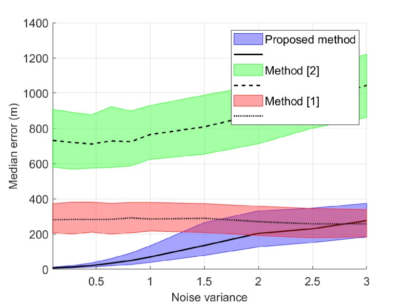
Figure 3: Median 3D-error (black lines) and 25th to 75th percentile (shaded areas) for the three different methods, for different measurement noise powers.

Figure 3 shows that our proposed algorithm, together with the method [2], perform worse with increasing noise power while method [1] does not. Method [2] yields an error that is around 700 meters larger than the error of the proposed algorithm throughout the tested noise interval, while the error of the proposed algorithm rises to a similar level to that of method [1] when the noise variance increases. The reason that the algorithm of [1] is independent of measurement noise is that it exploits the receiver positions only, and the centroid of the jammed receivers does not depend on the noise power.

IV-C Initial Value of ${\boldsymbol{\zeta}}$

The initial value of the parameter ${\boldsymbol{\zeta}}$ in the optimization is difficult to set adequatly without further information. To check how much the initial value of ${\boldsymbol{\zeta}}$ affects the result, a test is made where the gradient descent is initiated with different values of ${\boldsymbol{\zeta}}$. Five values between ${10}^{7}\text{\,}$ and ${10}^{9}\text{\,}$ are tested. Seven receivers are used, otherwise the settings used in Section IV-A are unchanged. The results can be seen in Figure 4.

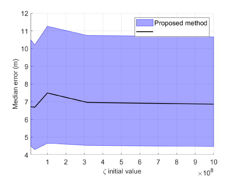
Figure 4: Median 3D-error (black lines) for our method using different initial values on $\zeta$, together with the 25th to 75th percentile (shaded areas).

Figure 4 shows that the initial value of ${\boldsymbol{\zeta}}$ does not affect the error much, and can therefore be set rather arbitrarily.

IV-D CNIR results

For the model using CNIR values, the same tests as in Section IV-A (excluding the road scenario) and Section IV-B were executed, testing both how the number of receivers and the measurement noise power affect the result. The same settings as for the AGC are used, except that the noise power is set to $\sigma_{S_{i,j}}^{2}=1$ and the range when testing different noise power levels is changed, going from 1 to 5. The results can be seen in Figure 5 and Figure 6, which show similar results as previously shown for the AGC-based algorithms. The methods are not affected by the noise as much as before, because the noise is added on each satellite signal, and only the mean of all satellite signals is used.

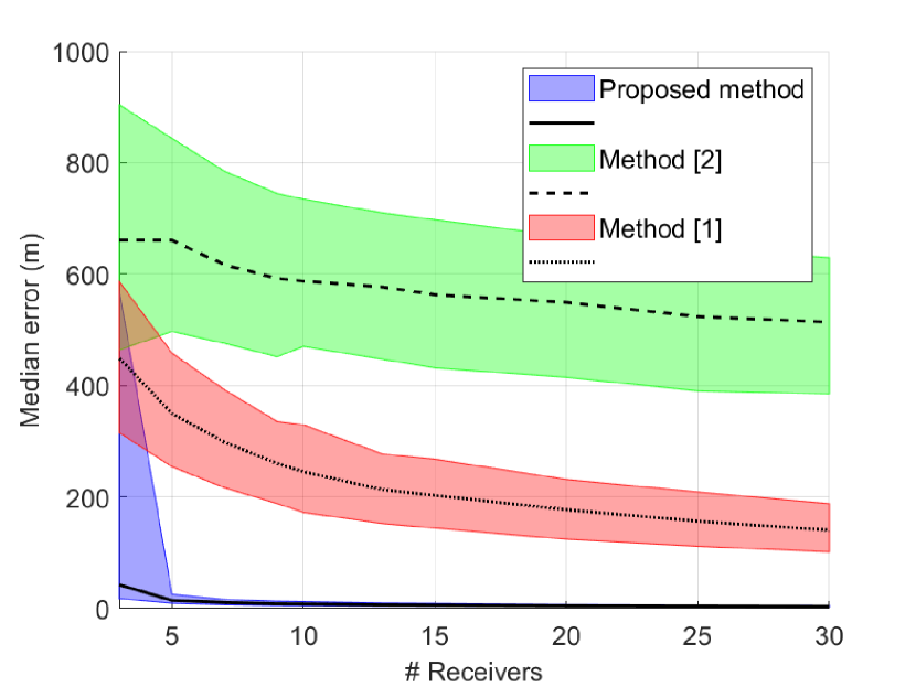
Figure 5: Median 3D-error (black lines) and 25th to 75th percentile (shaded areas) for the three different methods, using different number of receivers.

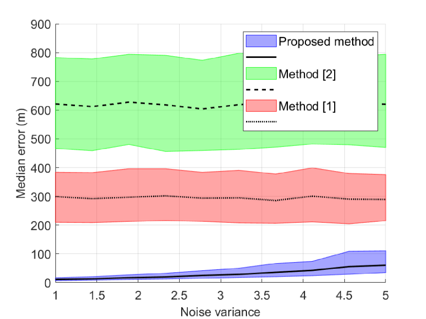
Figure 6: Median 3D-error (black lines) for the three different methods using different noise powers, together with the 25th to 75th percentile (shaded areas).

V Concluding Remarks

The proposed jamming localization algorithm, based on participatory sensing using AGC and $C/N_{0}$ estimates from commercial GNSS receivers, were shown to perform well in relevant scenarios. It was shown to outperform similar state-of-the-art localization algorithms, that are also based on participatory use of embedded GNSS receivers. The proposed method gives an estimation error below 15 meters using AGC or CNIR measurements from only 5 receivers, compared with hundreds of meters for the compared similar state-of-the-art localization methods. This is done without any prior knowledge of the jammer or path loss model.

Participatory receivers can be located anywhere and usually not in a controllable manner. It was shown that the proposed algorithm performs well for different receiver positions, placed randomly around the jammer or along a straight line, such as a road, next to the jammer. It should be noted that the proposed model has been evaluated with simulated data only, and the next step should be to test it using real measurements from GNSS receivers in real life scenarios.

References

- [1] D. Borio, C. Gioia, A. Štern, F. Dimc, and G. Baldini, “Jammer localization: From crowdsourcing to synthetic detection,” in Proc. ION GNSS+, 2016.
- [2] N. Ahmed and N. Sokolova, “RFI localization in a collaborative navigation environment,” in Proc. Int. Conf. on Localization and GNSS, 2020.
- [3] N. Ahmed, A. Winter, and N. Sokolova, “Low cost collaborative jammer localization using a network of UAVs,” in IEEE Aerospace Conference, 2021, pp. 1–8.
- [4] J. Liu, J. Xie, X. Zhang, and J. Wang, “Jammer localization approach based on crowdsourcing carrier-to-noise density power ratio fusion,” in Proc. China Satellite Navigation Conference (CSNC), 2020, pp. 604–612.
- [5] P. Wang and Y. T. Morton, “Efficient weighted centroid technique for crowdsourcing GNSS RFI localization using differential RSS,” IEEE Trans. Aerosp. Electron. Syst., vol. 56, no. 3, pp. 2471–2477, 2020.
- [6] J. A. Tucker, C. Puskar, C. Lee, and D. Akos, “GPS/GNSS interference power difference of arrival (PDOA) localization weighted via nearest neighbors,” in Proc. ION GNSS+, 2020.
- [7] R. C. Blay and D. M. Akos, “GNSS RFI localization using a hybrid TDOA/PDOA approach,” in Proc. ION International Technical Meeting (ITM), 2018.
- [8] L. Strizic, D. Akos, and S. Lo, “Crowdsourcing GNSS jammer detection and localization,” in Proc. ION International Technical Meeting (ITM), 2018, pp. 626–641.
- [9] I. Kraemer, P. Dykta, R. Bauernfeind, and B. Eissfeller, “Android GPS jammer localizer application based on C/N0 measurements and pedestrian dead reckoning,” in Proc. ION GNSS, 2012.
- [10] S. Gisdakis, T. Giannetsos, and P. Papadimitratos, “Security, Privacy, and Incentive Provision for Mobile Crowd Sensing Systems,” IEEE Internet of Things Journal (IEEE IoT), vol. 3, no. 5, pp. 839–853, October 2016.
- [11] ——, “SHIELD: A Data Verification Framework for Participatory Sensing Systems,” in ACM Conference on Security & Privacy in Wireless and Mobile Networks (ACM WiSec), New York, NY, USA, June 2015, pp. 16:1–16:12.
- [12] R. J. R. Thompson, E. Cetin, and A. G. Dempster, “Detection and jammer-to-noise ratio estimation of interferers using the automatic gain control,” in Proc. IGNSS symposium, 2011.
- [13] R. J. R. Thompson, “Detection and localisation of radio frequency interference to GNSS reference stations,” University of New South Wales, PhD dissertation, 2013.
- [14] D.-K. Lee, N. Spens, B. Gattis, and D. Akos, “AGC on Android devices for GNSS,” in Proc. ION International Technical Meeting (ITM), 2021, pp. 33–41.
- [15] M. J. Murrian, L. Narula, and T. E. Humphreys, “Characterizing terrestrial GNSS interference from low earth orbit,” in Proc. ION GNSS+, 2019.
- [16] L. Armijo, “Minimization of functions having Lipschitz continuous first partial derivatives,” Pacific Journal of Mathematics, vol. 16, no. 1, pp. 1 – 3, 1966.