h KA-TP-13-2022
Electroweak Phase Transition
in a Dark Sector with CP Violation

Abstract

In this paper, we investigate the possibility of a strong first-order electroweak phase transition (SFOEWPT) in the model ‘CP in the Dark’. The Higgs sector of the model consists of two scalar doublets and one scalar singlet with a specific discrete symmetry. After spontaneous symmetry breaking the model has a Standard-Model-like phenomenology and a hidden scalar sector with a viable Dark Matter candidate supplemented by explicit CP violation that solely occurs in the hidden sector. The model ‘CP in the Dark’ has been implemented in the C++ code BSMPT v2.3 which performs a global minimisation of the finite-temperature one-loop corrected effective potential and searches for SFOEWPTs. An SFOEWPT is found to be allowed in a broad range of the parameter space. Furthermore, there are parameter scenarios where spontaneous CP violation is generated at finite temperature. The in addition spontaneously broken $\mathbb{Z}_{2}$ symmetry then leads to mixing between the dark and the visible sector so that CP violation in the dark is promoted at finite temperature to the visible sector and thereby provides additional sources of CP violation that are not restricted by the electric dipole moment measurements at zero temperature. Thus, ‘CP in the Dark’ provides a promising candidate for the generation of the baryon asymmetry of the universe through electroweak baryogenesis.

1 Introduction

The discovery of the Higgs boson by the LHC experiments ATLAS [1] and CMS [2] structurally completes the Standard Model (SM) of particle physics. While the discovery of the 125 GeV scalar which behaves very SM-like marked a milestone for elementary particle physics, the SM itself leaves a lot of open problems to be explained. Many extensions beyond the SM, often entailing enlarged Higgs sectors, have been proposed to explain e.g. the existence of Dark Matter (DM) or the matter-antimatter asymmetry of the universe [3]. The latter can be explained through the mechanism of electroweak baryogenesis (EWBG) [4, 5, 6, 7, 8, 9, 10, 11, 12] provided the three Sakharov conditions [13] are fulfilled. These require baryon number violation, C and CP violation and departure from the thermal equilibrium. The asymmetry can be generated if the electroweak phase transition (EWPT), which proceeds through bubble formation, is of strong first order [10, 12]. In this case, the baryon number violating sphaleron transitions in the false vacuum are sufficiently suppressed [14, 15]. While in the SM in principle all Sakharov conditions are met, it can provide a strong first-order EWPT (SFOEWPT) only for a Higgs boson mass around 70-80 GeV [16, 17]. Moreover, the amount of CP violation in the SM, originating from the Cabibbo-Kobayashi-Maskawa (CKM) matrix in not large enough to quantitatively reproduce the measured matter-antimatter asymmetry [12, 18].

In this paper, we investigate the model ‘CP in the Dark’ with respect to two of the above-mentioned open problems of the SM, namely Dark Matter and the observed matter-antimatter asymmetry. The model has been proposed for the first time in [19]. It consists of a 2-Higgs-Doublet Model (2HDM) [20, 21] Higgs sector extended by a real singlet field, hence a Next-to-2HDM (N2HDM). Compared to the N2HDM studied in [22] it uses a different discrete symmetry. The symmetry is designed such that it leads to the following interesting properties of the model: $(i)$ an SM-like Higgs boson $h$ that is naturally aligned because of the vacuum of the model preserving the chosen discrete symmetry; $(ii)$ a viable DM candidate with its stability being guaranteed by the vacuum of the model and with its mass and couplings satisfying all existing DM search constraints; $(iii)$ extra sources of CP violation existing solely in the ’dark’ sector. Because of this hidden CP violation, which is explicit, the SM-like Higgs $h$ behaves almost exactly like the SM Higgs boson, its couplings to massive gauge bosons and fermions are exactly those of the SM Higgs (modulo contributions from a high number of loops). In [19] we investigated the phenomenology of the model with respect to collider and DM observables. We discussed how the hidden CP violation might be tested at future colliders, namely through anomalous gauge couplings.

This hidden CP violation can be very interesting in the context of EWBG. First of all, with the extended Higgs sector of ‘CP in the Dark’ we have the chance to generate an SFOEWPT. Second, the fact that CP violation does not occur in the visible sector at zero temperature means that it is not constrained by the strict bounds from the electric dipole moment (EDM) measurements. This means in turn that CP violation in the dark sector can take any value without being in conflict with experiment. If this CP violation can be translated to the visible sector we have very powerful means to enhance the generated baryon asymmetry of the universe (BAU) through a large amount of CP violation. Additionally, the model provides a viable DM candidate so that we are able to solve two of the most prominent open questions than cannot be resolved within the SM.

In this paper, we investigate the model ‘CP in the Dark’ with respect to its potential of generating an SFOEWPT. We furthermore analyse whether the CP violation in the dark sector can be transmitted at finite temperature to the visible sector and thereby improve the conditions of generating a baryon asymmetry large enough to match the experimental value. It turns out that at finite temperature both CP violation and violation of the discrete symmetry are generated spontaneously through the appearance of the corresponding non-vanishing vacuum expectation values. This allows the transmission of CP violation from the dark to the visible Higgs sector. Note that in our investigation we take into account all relevant theoretical and experimental constraints. We find in particular that our model not only provides an SFOEWPT with possibly spontaneous CP violation but also complies with all constraints from DM observables.

The structure of the paper is as follows. We start by introducing the model ‘CP in the Dark’ in Sec. 2. In Sec. 3 the calculation of the strength of the EWPT, as well as the chosen renormalisation prescription is described. In Sec. 4 we describe our procedure to generate viable parameter points for our numerical analysis. We show and discuss our results in Sec. 5 and conclude in Sec. 6.

2 CP in the Dark

The model ‘CP in the Dark’ proposed in [19] is a specific version of the N2HDM [25, 22, 26] which features an extended scalar sector with two scalar doublets $\Phi_{1}$ and $\Phi_{2}$ and a real scalar singlet $\Phi_{S}$. In contrast to the N2HDM discussed in [22], however, the Lagrangian is required to be invariant under solely one discrete $\mathbb{Z}_{2}$ symmetry, namely

$$\Phi_{1}\rightarrow\Phi_{1}\,,\quad\Phi_{2}\rightarrow-\Phi_{2}\,,\quad\Phi_{S}\rightarrow-\Phi_{S}\,.$$ (2.1)

With the Yukawa sector considered to be neutral under this symmetry, therefore only one of the two doublets, $\Phi_{1}$, couples to the fermions so that the absence of scalar-mediated tree-level flavour-changing neutral currents (FCNC) is automatically ensured, and the Yukawa sector is identical to the SM one. With this $\mathbb{Z}_{2}$ symmetry, the most general scalar tree-level potential invariant under $\mathrm{SU}(2)_{L}\times\mathrm{U}(1)_{Y}$ reads

$$\begin{split}V^{(0)}\,=\,\,\,&m_{11}^{2}|\Phi_{1}|^{2}+m_{22}^{2}|\Phi_{2}|^{2}+\frac{m_{S}^{2}}{2}\Phi_{S}^{2}+\left(A\Phi_{1}^{\dagger}\Phi_{2}\Phi_{S}+\text{ h.c.}\right)\\ &+\frac{\lambda_{1}}{2}|\Phi_{1}|^{4}+\frac{\lambda_{2}}{2}|\Phi_{2}|^{4}+\lambda_{3}|\Phi_{1}|^{2}|\Phi_{2}|^{2}+\lambda_{4}|\Phi_{1}^{\dagger}\Phi_{2}|^{2}+\frac{\lambda_{5}}{2}[(\Phi_{1}^{\dagger}\Phi_{2})^{2}+(\Phi_{2}^{\dagger}\Phi_{1})^{2}]\\ &+\frac{\lambda_{6}}{4}\Phi_{S}^{4}+\frac{\lambda_{7}}{2}|\Phi_{1}|^{2}\Phi_{S}^{2}+\frac{\lambda_{8}}{2}|\Phi_{2}|^{2}\Phi_{S}^{2}\,.\end{split}$$ (2.2)

All parameters of the potential are real, except for the trilinear coupling $A$. A possible complex phase of the quartic coupling $\lambda_{5}$ is absorbed by a proper rotation of the doublet fields [19]. After electroweak symmetry breaking (EWSB), the scalar doublets and the singlet can be expanded around the vacuum expectation values (VEVs). Allowing for the most general vacuum structure where besides the doublet and singlet VEVs $\overline{\omega}_{1,2}$ and $\overline{\omega}_{S}$, respectively, we take into account also CP-violating ($\overline{\omega}_{\text{CP}}$) and charge-breaking ($\overline{\omega}_{\text{CB}}$) VEVs, we have

$$\Phi_{1}=\frac{1}{\sqrt{2}}\begin{pmatrix}\rho_{1}+i\eta_{1}\\ \zeta_{1}+\overline{\omega}_{1}+i\Psi_{1}\end{pmatrix}\,,\quad\Phi_{2}=\frac{1}{\sqrt{2}}\begin{pmatrix}\rho_{2}+\overline{\omega}_{\text{CB}}+i\eta_{2}\\ \zeta_{2}+\overline{\omega}_{2}+i(\Psi_{2}+\overline{\omega}_{\text{CP}})\end{pmatrix}\,,\quad\Phi_{S}=\zeta_{S}+\overline{\omega}_{\text{S}}\,.$$ (2.3)

Here we introduced the charged CP-even and CP-odd fields $\rho_{i}$ and $\eta_{i}$ as well as the neutral CP-even and CP-odd fields $\zeta_{i}$ and $\Psi_{i}$ ($i=1,2$). The zero-temperature vacuum structure is chosen such that the imposed $\mathbb{Z}_{2}$-symmetry remains unbroken, i.e.

$$\langle\Phi_{1}\rangle|_{T=$0\text{\,}\mathrm{G}\mathrm{e}\mathrm{V}$}=\frac{1}{\sqrt{2}}\begin{pmatrix}0\\ v_{1}\end{pmatrix},\quad\langle\Phi_{2}\rangle|_{T=$0\text{\,}\mathrm{G}\mathrm{e}\mathrm{V}$}=\begin{pmatrix}0\\ 0\end{pmatrix}\quad\text{and}\quad\langle\Phi_{S}\rangle|_{T=$0\text{\,}\mathrm{G}\mathrm{e}\mathrm{V}$}=0\,,$$ (2.4)

with $\overline{\omega}_{1}|_{T=$0\text{\,}\mathrm{G}\mathrm{e}\mathrm{V}$}\equiv v_{1}\equiv v\approx$246.22\text{\,}\mathrm{G}\mathrm{e}\mathrm{V}$$. Since only the first Higgs doublet couples to fermions, $\Phi_{1}$ is the SM-like doublet and provides an SM-like Higgs boson $h$. The first doublet can be written in terms of the mass eigenstates as

$$\Phi_{1}=\begin{pmatrix}G^{+}\\ \frac{1}{\sqrt{2}}\left(h+v_{1}+iG^{0}\right)\end{pmatrix}\,,$$ (2.5)

where $G^{+}$ denotes the massless charged and $G^{0}$ the massless neutral Goldstone boson, respectively. The upper charged components of the second doublet $\Phi_{2}$ provide the charged mass eigenstate $H^{+}$. The neutral fields $\zeta_{2}$, $\Psi_{2}$ and $\zeta_{S}$ mix, with the corresponding mixing matrix given by

$$M_{N}^{2}=\begin{pmatrix}m_{22}^{2}+\frac{v_{1}^{2}}{2}\lambda_{345}&0&\operatorname{Re}\,(A)v_{1}\\ 0&m_{22}^{2}+\frac{v_{1}^{2}}{2}\overline{\lambda}_{345}&-\operatorname{Im}\,(A)v_{1}\\ \operatorname{Re}\,(A)v_{1}&-\operatorname{Im}\,(A)v_{1}&m_{S}^{2}+\frac{v_{1}^{2}}{2}\lambda_{7}\\ \end{pmatrix}\,,$$ (2.6)

where we have introduced $\lambda_{345}\equiv\lambda_{3}+\lambda_{4}+\lambda_{5}$ and $\overline{\lambda}_{345}\equiv\lambda_{3}+\lambda_{4}-\lambda_{5}$. Diagonalisation with the rotation matrix $R$ yields the mass eigenvalues $h_{i}$ ($i=1,2,3$),

$$\text{diag}(m_{h_{1}}^{2},m_{h_{2}}^{2},m_{h_{3}}^{2})=RM_{N}^{2}R^{T}\,,$$ (2.7)

which by convention are ordered by ascending mass, $m_{h_{1}}\leq m_{h_{2}}\leq m_{h_{3}}$. The orthogonal matrix $R$ can be parametrised in terms of three mixing angles $\alpha_{i}$ ($i=1,2,3$),

$$R=\begin{pmatrix}c_{\alpha_{1}}c_{\alpha_{2}}&s_{\alpha_{1}}c_{\alpha_{2}}&s_{\alpha_{2}}\\ -(c_{\alpha_{1}}s_{\alpha_{2}}s_{\alpha_{3}}+s_{\alpha_{1}}c_{\alpha_{3}})&c_{\alpha_{1}}c_{\alpha_{3}}-s_{\alpha_{1}}s_{\alpha_{2}}s_{\alpha_{3}}&c_{\alpha_{2}}s_{\alpha_{3}}\\ -c_{\alpha_{1}}s_{\alpha_{2}}c_{\alpha_{3}}+s_{\alpha_{1}}s_{\alpha_{3}}&-(c_{\alpha_{1}}s_{\alpha_{3}}+s_{\alpha_{1}}s_{\alpha_{2}}c_{\alpha_{3}})&c_{\alpha_{2}}c_{\alpha_{3}}\end{pmatrix}\,.$$ (2.8)

Note that the chosen vacuum at zero temperature given in Eq. (2.4) does not include a CP-violating VEV. As mentioned above, the zero-temperature vacuum also conserves the $\mathbb{Z}_{2}$ symmetry of Eq. (2.1), introducing a conserved quantum number, called dark charge. While all SM-like particles have dark charge $+1$, the charged scalar $H^{+}$ and the neutral scalars $h_{1,2,3}$ that originate from the second doublet $\Phi_{2}$, and the real singlet $\Phi_{S}$, have dark charge $-1$. They are called dark particles. The lightest neutral dark particle $h_{1}$ therefore acts as a stable dark matter candidate. ‘CP in the Dark’ additionally features explicit CP violation in the dark sector which is introduced through $\operatorname{Im}A\neq 0$. For further details, we refer to [19].

The model ‘CP in the Dark’ is determined by thirteen input parameters. Exploiting the minimum condition

$$m_{11}^{2}+\frac{1}{2}\lambda_{1}v_{1}^{2}=0$$ (2.9)

to trade $m_{11}^{2}$ for $v_{1}$, we use the following input parameters for the parameter scan performed with ScannerS [27, 28, 22, 29], cf. Sec. 4,

$$m_{h}\,,\ m_{h_{1}}\,,\ m_{h_{2}}\,,\ m_{H^{\pm}}\,,\ v_{1}\,,\ m_{22}^{2}\,,\ m_{S}^{2}\,,\ \alpha_{1}\,,\ \alpha_{2}\,,\ \alpha_{3}\,,\ \lambda_{2}\,,\ \lambda_{6}\;,\ \lambda_{8}\;.$$ (2.10)

For our program BSMPT [30, 31] used to compute the EWPT of the model, we use the default input set of BSMPT,

$$m_{h}\,,\ m_{S}^{2}\,,\ m_{22}^{2}\,,\ v_{1}\,,\ \operatorname{Re}A\,,\ \operatorname{Im}A\,,\ \lambda_{2}\,,\ \lambda_{3}\,,\ \lambda_{4}\,,\ \lambda_{5}\,,\ \lambda_{6}\,,\ \lambda_{7}\,,\ \lambda_{8}\;.$$ (2.11)

3 Calculation of the Strength of the Phase Transition

We follow the approach of Refs. [32, 33, 34] to determine the strength $\xi_{c}$ of the EWPT. It is given by the ratio of the critical VEV $v_{c}$ at the critical temperature $T_{c}$, $\xi_{c}=v_{c}/T_{c}$. The critical temperature is defined as the temperature where the symmetric and the broken minimum are degenerate, hence

$$V(v=0,T_{c})=V(v=v_{c},T_{c})\,,$$ (3.12)

with the critical VEV determined as $v_{c}\equiv v(T)\big{|}_{T=T_{c}}$, see below. A value larger than one is indicative for a strong first-order EWPT [7, 35]. For the determination of $\xi_{c}$ we use the C++ program BSMPT [30, 31] where we implemented the daisy-corrected one-loop effective potential at finite temperature of ‘CP in the Dark’. ‘CP in the Dark’ was implemented as a new model class in BSMPT, which is publicly available since version 2.3. Since the corresponding details of the calculation do not differ compared to the other models, we refer to our previous publications for further details, cf. [30, 31]. However, note that we had to adapt the proposed renormalisation scheme applied in the previous publications, which we will discuss in the following.

For an efficient parameter scan, it is convenient to renormalise the loop-corrected masses and angles to their tree-level values. This is usually achieved by adapting the renormalisation scheme that has been introduced for the 2HDM in Ref. [32]. The scheme was further applied to the C2HDM and the N2HDM in [33, 30, 34, 40] and to the CxSM in [31]. In the following, we shortly summarise the procedure and adapt it to the model ‘CP in the Dark’. The one-loop corrected effective potential with one-loop masses and angles renormalised to their tree-level values is constructed as

$$V(\omega,T)=V^{(0)}(\omega)+V^{\text{CW}}(\omega)+V^{\text{T}}(\omega,T)+V^{\text{CT}}(\omega)\,.$$ (3.13)

The tree-level potential $V^{(0)}$ is given in Eq. (2.2) with the doublet and singlet fields replaced by the classical constant field configurations $\Phi_{1}^{c}=(0,\omega_{1}/\sqrt{2})^{T}$, $\Phi_{2}^{c}=1/\sqrt{2}\,(\omega_{\text{CB}},\omega_{2}+i\omega_{\text{CP}})^{T}$ and $\Phi_{S}^{c}=\omega_{S}$, respectively. The Coleman-Weinberg potential is denoted by $V^{\text{CW}}(\omega)$, the contribution $V^{\text{T}}(\omega,T)$ accounts for the thermal corrections at finite temperature, and the counterterm potential $V^{\text{CT}}(\omega)$ is given by [32]

$$V^{\text{CT}}=\sum_{i=1}^{N_{p}}\frac{\partial V^{(0)}}{\partial p_{i}}\delta p_{i}+\sum_{k=1}^{N_{v}}\delta T_{k}(\phi_{k}+\omega_{k})\,.$$ (3.14)

The number of parameters $p_{i}$ of the tree-level potential is denoted by $N_{p}$. The finite counterterm parameters are referred to as $\delta p_{i}$. Additionally, a tadpole counterterm $\delta T_{k}$ for each of the $N_{v}=5$ field directions that are allowed to develop a non-zero VEV is included. Applying Eq. (3.14) to the tree-level potential of ‘CP in the Dark’ of Eq. (2.2) results in

$$V^{\text{CT}} = \delta m_{11}^{2}|\Phi_{1}|^{2}+\delta m_{22}^{2}|\Phi_{2}|^{2}+\frac{\delta m_{S}^{2}}{2}\Phi_{S}^{2}$$ (3.15)

$$+ [\delta\operatorname{Re}\,(A)+i\delta\operatorname{Im}\,(A)]\Phi_{1}^{\dagger}\Phi_{2}\Phi_{S}+[\delta\operatorname{Re}\,(A)-i\delta\operatorname{Im}\,(A)]\Phi_{S}\Phi_{2}^{\dagger}\Phi_{1}$$

$$+ \frac{\delta\lambda_{1}}{2}|\Phi_{1}|^{4}+\frac{\delta\lambda_{2}}{2}|\Phi_{2}|^{4}+\delta\lambda_{3}|\Phi_{1}|^{2}|\Phi_{2}|^{2}+\delta\lambda_{4}|\Phi_{1}^{\dagger}\Phi_{2}|^{2}+\frac{\delta\lambda_{5}}{2}[(\Phi_{1}^{\dagger}\Phi_{2})^{2}+(\Phi_{2}^{\dagger}\Phi_{1})^{2}]$$

$$+ \frac{\delta\lambda_{6}}{4}\Phi_{S}^{4}+\frac{\delta\lambda_{7}}{2}|\Phi_{1}|^{2}\Phi_{S}^{2}+\frac{\delta\lambda_{8}}{2}|\Phi_{2}|^{2}\Phi_{S}^{2}$$

$$+ \delta T_{\text{CB}}(\rho_{2}+\omega_{\text{CB}})+\delta T_{1}(\zeta_{1}+\omega_{1})$$

$$+ \delta T_{2}(\zeta_{2}+\omega_{2})+\delta T_{\text{CP}}(\Psi_{2}+\omega_{\text{CP}})+\delta T_{\text{S}}(\zeta_{S}+\omega_{\text{S}})\,.$$

The counterterm parameters $\delta p_{i}$ and $\delta T_{k}$ are determined through the renormalisation conditions

$$\partial_{\phi_{i}}\left(V^{\text{CT}}+V^{\text{CW}}\right)\big{|}_{\phi=\langle\phi^{c}\rangle|_{T=$0\text{\,}\mathrm{G}\mathrm{e}\mathrm{V}$}}=0$$ (3.16a)

$$\partial_{\phi_{i}}\partial_{\phi_{j}}\left(V^{\text{CT}}+V^{\text{CW}}\right)\big{|}_{\phi=\langle\phi^{c}\rangle|_{T=$0\text{\,}\mathrm{G}\mathrm{e}\mathrm{V}$}}=0\,.$$ (3.16b)

In the following, we use the notation $N^{\text{CW}}_{\phi}\equiv\partial_{\phi}V^{\text{CW}}$ and $H^{\text{CW}}_{\phi_{i}\phi_{j}}\equiv\partial_{\phi_{i}\phi_{j}}V^{\text{CW}}$. The scalar fields $\phi_{i}$ in the gauge basis are labelled as

$$\phi_{i}=\{\rho_{1},\eta_{1},\rho_{2},\eta_{2},\zeta_{1},\Psi_{1},\zeta_{2},\Psi_{2},\zeta_{S}\}\,.$$ (3.17)

The field configuration at $T=0$ GeV is denoted by $\langle\phi^{c}\rangle|_{T=$0\text{\,}\mathrm{G}\mathrm{e}\mathrm{V}$}$ and given by

$$\langle\phi^{c}\rangle|_{T=$0\text{\,}\mathrm{G}\mathrm{e}\mathrm{V}$}=\{0,0,0,0,v_{1},0,0,0,0\}\quad\text{and}\quad v_{1}\equiv v\approx$246.22\text{\,}\mathrm{G}\mathrm{e}\mathrm{V}$\,.$$ (3.18)

The renormalisation conditions of Eq. (3.16) yield an overconstrained system of equations. Its five-dimensional solution space can be parametrised by $\delta\lambda_{i}\equiv t_{i}\in\mathbb{R}$ ($i=2,3,6,7,8$) so that we have

$$\delta m_{11}^{2} =\frac{1}{2}H^{\text{CW}}_{\zeta_{1}\zeta_{1}}-\frac{3}{2}H^{\text{CW}}_{\rho_{1}\rho_{1}}$$ (3.19a)

$$\delta m_{22}^{2} =-H^{\text{CW}}_{\rho_{2}\rho_{2}}-\frac{1}{2}t_{3}v_{1}^{2}$$ (3.19b)

$$\delta m_{S}^{2} =-H^{\text{CW}}_{\zeta_{S}\zeta_{S}}-\frac{1}{2}t_{7}v_{1}^{2}$$ (3.19c)

$$\delta\operatorname{Re}\,(A) =-\frac{1}{v_{1}}H^{\text{CW}}_{\zeta_{2}\zeta_{S}}$$ (3.19d)

$$\delta\operatorname{Im}\,(A) =\frac{1}{v_{1}}H^{\text{CW}}_{\Psi_{2}\zeta_{S}}$$ (3.19e)

$$\delta\lambda_{1} =\frac{1}{v_{1}^{2}}\left(-H^{\text{CW}}_{\zeta_{1}\zeta_{1}}+H^{\text{CW}}_{\rho_{1}\rho_{1}}\right)$$ (3.19f)

$$\delta\lambda_{2} =t_{2}$$ (3.19g)

$$\delta\lambda_{3} =t_{3}$$ (3.19h)

$$\delta\lambda_{4} =\frac{1}{v_{1}^{2}}\left(2H^{\text{CW}}_{\rho_{2}\rho_{2}}-H^{\text{CW}}_{\zeta_{2}\zeta_{2}}-H^{\text{CW}}_{\Psi_{2}\Psi_{2}}\right)$$ (3.19i)

$$\delta\lambda_{5} =\frac{1}{v_{1}^{2}}\left(-H^{\text{CW}}_{\zeta_{2}\zeta_{2}}+H^{\text{CW}}_{\Psi_{2}\Psi_{2}}\right)$$ (3.19j)

$$\delta\lambda_{6} =t_{6}$$ (3.19k)

$$\delta\lambda_{7} =t_{7}$$ (3.19l)

$$\delta\lambda_{8} =t_{8}$$ (3.19m)

$$\delta T_{\text{CB}} =-N^{\text{CW}}_{\rho_{2}}$$ (3.19n)

$$\delta T_{1} =v_{1}H^{\text{CW}}_{\rho_{1}\rho_{1}}-N^{\text{CW}}_{\zeta_{1}}$$ (3.19o)

$$\delta T_{2} =-N^{\text{CW}}_{\zeta_{2}}$$ (3.19p)

$$\delta T_{\text{CP}} =-N^{\text{CW}}_{\Psi_{2}}$$ (3.19q)

$$\delta T_{\text{S}} =-N^{\text{CW}}_{\zeta_{S}}\,.$$ (3.19r)

Equation (3.19) provides a consistent solution to Eq. (3.16) only if additionally the following identities are fulfilled,

$$H^{\text{CW}}_{\rho_{1}\rho_{1}} =H^{\text{CW}}_{\Psi_{1}\Psi_{1}}$$ (3.20a)

$$H^{\text{CW}}_{\eta_{1}\eta_{1}} =H^{\text{CW}}_{\Psi_{1}\Psi_{1}}$$ (3.20b)

$$H^{\text{CW}}_{\rho_{2}\rho_{2}} =H^{\text{CW}}_{\eta_{2}\eta_{2}}.$$ (3.20c)

However, with $V^{\text{CT}}$ determined through Eq. (3.19) we still observe

$$\partial_{\zeta_{2}}\partial_{\Psi_{2}}\left(V^{\text{CW}}+V^{\text{CT}}\right)\big{|}_{\phi=\langle\phi^{c}\rangle|_{T=$0\text{\,}\mathrm{G}\mathrm{e}\mathrm{V}$}}\sim\mathcal{O}(10^{1}\mbox{ GeV}^{2})\,.$$ (3.21)

These non-cancelled second derivatives are due to field directions $ij=\{\zeta_{2}\Psi_{2}\}$ in which the Coleman-Weinberg potential yields non-zero contributions $\partial_{ij}^{2}V^{\text{CW}}$, but the counterterm potential with the ansatz of Eq. (3.15) vanishes, $\partial^{2}_{ij}V^{\text{CT}}=0$. Hence, there is no cancellation possible. Therefore, the solution of Eq. (3.19) is insufficient for these $ij$. The reason are loop-induced CP-violating couplings that lead to non-zero derivatives of $V^{\text{CW}}$ in field directions that are not present in the chosen $V^{\text{CT}}$ of Eq. (3.15). For ‘CP in the Dark’ we therefore propose a modified renormalisation scheme by adding one additional counterterm that parametrises the additional CP-violating structure

$$\widetilde{V}^{\text{CT}}\equiv V^{\text{CT}}+\frac{i}{2}\delta\operatorname{Im}(\lambda_{5})\left((\Phi_{1}^{\dagger}\Phi_{2})^{2}-(\Phi_{1}\Phi_{2}^{\dagger})^{2}\right)\,.$$ (3.22)

The new counterterm $\delta\operatorname{Im}(\lambda_{5})$ is constrained through Eq. (3.16) to be

$$\delta\operatorname{Im}\,(\lambda_{5})=\frac{2}{v_{1}^{2}}H^{\text{CW}}_{\zeta_{2}\Psi_{2}}\,.$$ (3.23)

Furthermore, we choose the free parameters for the solution to be $t_{i}=0$ for the analysis in Sec. 4. This choice corresponds to the renormalisation scheme with all additional finite pieces set to zero that are irrelevant for the initial aim of fixing next-to-leading order (NLO) masses and angles at their tree-level values.

By performing a global minimisation of the renormalised one-loop corrected effective potential, BSMPT calculates the critical temperature $T_{c}$ and the critical VEV $v_{c}$. For details, we refer to [30, 31]. The temperature-dependent electroweak VEV $v(T)$ is calculated taking into account all possible $SU(2)_{L}$ VEV contributions,

$$v(T)=\sqrt{\overline{\omega}_{1}^{2}(T)+\overline{\omega}_{2}^{2}(T)+\overline{\omega}_{\text{CP}}^{2}(T)+\overline{\omega}_{\text{CB}}^{2}(T)}\,.$$ (3.24)

Remind that the $\overline{\omega}_{i}$ are the field configurations that minimise the loop-corrected effective potential at non-zero temperature. We do not include the singlet VEV $\bar{\omega}_{S}$ in Eq. (3.24), but we take it into account for the minimisation procedure. The reason is that the electroweak sphaleron couples only to particles charged under $SU(2)_{L}$. In case the baryon-wash-out condition is fulfilled, i.e.

$$\xi_{c}=\frac{v_{c}}{T_{c}}\gtrsim 1\,,$$ (3.25)

the EWPT is an SFOEWPT and provides the necessary departure from thermal equilibrium as required by the Sakharov conditions.

4 Numerical Analysis

For our numerical analysis we perform a scan in the parameter space of the model and keep only those points that are compatible with the relevant theoretical and experimental constraints. We require the SM-like Higgs boson $h$ to have a mass of $m_{h}=125.09~{}\text{GeV}$ [41] and behave SM-like. The remaining input parameters of ‘CP in the Dark’ are varied in the ranges given in Tab. 1.

$m_{h}$	$m_{h_{1}}$	$m_{h_{2}}$	$m_{H^{\pm}}$	$m_{22}^{2}$	$m_{S}^{2}$
in  GeV	in  GeV	in  GeV	in  GeV	in $~{}\text{GeV}^{2}$	in $~{}\text{GeV}^{2}$
$125.09$	$\left[1,1000\right]$	$\left[1,1000\right]$	$\left[65,1000\right]$	$\left[0,10^{6}\right]$	$\left[0,10^{6}\right]$
$\alpha_{1}$	$\alpha_{2}$	$\alpha_{3}$	$\lambda_{2}$	$\lambda_{6}$	$\lambda_{8}$
$\left[-\frac{\pi}{2},\frac{\pi}{2}\right)$	$\left[-\frac{\pi}{2},\frac{\pi}{2}\right)$	$\left[-\frac{\pi}{2},\frac{\pi}{2}\right)$	$\left[0,9\right]$	$\left[0,17\right]$	$\left[-26,26\right]$

Table 1: Parameter scan ranges of the ‘CP in the Dark’ input parameters used in ScannerS.

For the SM parameters, we use the fine structure constant at the scale of the $Z$ boson mass [42, 43],

$$\alpha_{\text{EM}}^{-1}(M_{Z}^{2})=128.962\;,$$ (4.26)

and the masses for the massive gauge bosons are chosen as [42, 43]

$$m_{W}=80.385~{}\text{GeV}\quad\text{and }\quad m_{Z}=91.1876~{}\text{GeV}\,.$$ (4.27)

The lepton masses are set to [42, 43]

$$m_{e}=0.511~{}\mathrm{MeV},\quad m_{\mu}=105.658~{}\mathrm{MeV},\quad m_{\tau}=1.777~{}\text{GeV}\,,$$ (4.28)

and the light quark masses to [43]

$$m_{u}=m_{d}=m_{s}=100~{}\mathrm{MeV}\,.$$ (4.29)

To be consistent with the CMS and ATLAS analyses, we take the on-shell top quark mass as [43, 44]

$$m_{t}=172.5~{}\text{GeV}\,$$ (4.30)

and the recommended charm and bottom quark on-shell masses [43]

$$m_{c}=1.51~{}\text{GeV}\quad\text{and}\quad m_{b}=4.92~{}\text{GeV}\,.$$ (4.31)

We choose the complex parametrisation of the CKM matrix [45, 42],

$$V_{\text{CKM}}=\begin{pmatrix}c_{12}c_{13}&s_{12}c_{13}&s_{13}\mathrm{e}^{-\mathrm{i}\delta}\\ -s_{12}c_{23}-c_{12}s_{23}s_{13}\mathrm{e}^{\mathrm{i}\delta}&c_{12}c_{23}-s_{12}s_{23}s_{13}\mathrm{e}^{\mathrm{i}\delta}&s_{23}c_{13}\\ s_{12}s_{23}-c_{12}c_{23}s_{13}\mathrm{e}^{\mathrm{i}\delta}&-c_{12}s_{23}-s_{12}c_{23}c_{13}\mathrm{e}^{\mathrm{i}\delta}&c_{23}c_{13}\end{pmatrix}\,,$$ (4.32)

where $s_{ij}\equiv\sin\theta_{ij}$ and $c_{ij}\equiv\cos\theta_{ij}$. The angles are given in terms of the Wolfenstein parameters as

$$s_{12}=\lambda\,,\quad s_{13}\mathrm{e}^{\mathrm{i}\delta}=A\lambda^{3}\left(\rho+\mathrm{i}\eta\right)\,,\quad s_{23}=A\lambda^{2}\,,$$ (4.33)

with [34]

$$\lambda=0.22537\,, A=0.814\;, \rho=0.117\;, \eta=0.353\,.$$ (4.34)

Note that we take into account a complex phase $\delta$ in the CKM matrix as an additional source for CP violation. The impact of the complex CKM phase compared to that of the complex phase induced by the VEV configuration is negligible, however. Finally, the electroweak VEV is set to

$$v_{1}\equiv v=1/\sqrt{\sqrt{2}G_{F}}\approx 246.22~{}\text{GeV}\,.$$ (4.35)

The parameter points under investigation have to fulfil experimental and theoretical constraints. For the generation of such parameter points we use the C++ program ScannerS [27, 28, 22, 29]. ScannerS allows us to check for boundedness from below of the tree-level potential and uses the tree-level discriminant of [46] to ensure the electroweak vacuum to be the global minimum at tree level. It also checks for perturbative unitarity. By using BSMPT it is also possible to check for the NLO electroweak vacuum to be the global minimum of the potential. Only parameter points providing a stable NLO electroweak vacuum at zero temperature are taken into account for the analysis. The check for consistency with recent flavour constraints is obsolete since in ‘CP in the Dark’ the charged Higgs boson belongs to the dark sector and does not couple to fermions so that all $B$-physics constraints are fulfilled per default. The compatibility with the Higgs measurements is taken into account by ScannerS through HiggsBounds [47, 48, 49, 50, 51, 52] and HiggsSignals [53, 54]. For the parameter scan the versions HiggsBounds5.9.0 and HiggsSignals2.6.1 are used. We have also taken into account the latest CMS results [55] on the Higgs signal strength in the photonic final state that were not implemented in HiggsSignals. We have checked the compatibility with the recent ATLAS result on the Higgs decay into invisible particles, $\text{BR}(h\rightarrow\,\text{inv.})<$0.11$$ [56]. Further Dark Matter observables like the spin-independent DM-nucleon cross section and the relic abundance are checked with MicrOMEGAs5.2.7a [57, 58, 59, 60, 61, 62, 63, 64, 65, 66]. We demand that our parameter scenarios do not lead to relic densities above the experimentally measured value of [67]

$$\Omega_{\text{obs}}h^{2}=0.1200\pm 0.0012\,,$$ (4.36)

while they may be below the value assuming other DM particles beyond our model to saturate the relic density. Note that we need not check for the strict constraints on CP violation arising from the electric dipole moment measurements, where the stringest one is provided by the ACME collaboration [68], as in our model CP violation beyond the SM arises only in the dark sector. For the determination of the strength of the EWPT we use the new model implementation in BSMPT v2.3 [30, 31]. The code can be downloaded from the url:

https://github.com/phbasler/BSMPT.

5 Results

In this section, we present our numerical results. We start with the discussion of the visible sector of ‘CP in the Dark’, namely in Sec. 5.1 with the discussion of the impact of the applied constraints on the branching ratios and signal strengths of the SM-like Higgs boson in the context of the additional dark sector. We further discuss the impact of the strength of the phase transition. Subsequently, we investigate in Sec. 5.2 the mass distributions of our dark sector particles and if there is an interplay between their masses and the requirement of an SFOEWPT. We then analyse in detail in Sec. 5.3 the VEV configurations that were found to minimise the one-loop corrected effective potential at finite temperature. Special attention is paid here on the spontaneous generation of CP violation. In Sec. 5.4 finally we show results for the DM observables and study their interplay with the requirement of an SFOEWPT.

5.1 Branching Ratios and Signal Strengths of the SM-like Higgs Boson

Since the tree-level couplings of the SM-like Higgs $h$ in our model are identical to those of the SM Higgs boson, it is only the presence of the dark particles that can change the branching ratios of $h$. Thus, the dark charged Higgs boson can contribute to the decay width into a photon pair, cf. [19], so that the decay width $\Gamma(h\to\gamma\gamma)$ is changed. Furthermore, $h$ can decay into a pair of DM particles if kinematically allowed which would change the total width and hence also the branching ratio.

In Fig. 1 we show the branching ratio of the SM-like Higgs into two photons normalised to the branching ratio of the SM Higgs boson as a function of the dark charged Higgs mass. Neglecting subdominant electroweak corrections, the production cross section of the SM-like Higgs, $\sigma_{\text{prod}}(h)$, is not changed with respect to that of the SM Higgs boson so that the ratio of the branching ratios directly corresponds to the signal rate $\mu_{\gamma\gamma}$,

$$\mu_{\gamma\gamma}\equiv\frac{\sigma_{\text{prod}}(h)\times\mbox{BR}(h\to\gamma\gamma)}{\sigma_{\text{prod}}^{\text{SM}}(h)\times\mbox{BR}^{\text{SM}}(h\to\gamma\gamma)}\equiv\frac{\mbox{BR}(h\to\gamma\gamma)}{\mbox{BR}^{\text{SM}}(h\to\gamma\gamma)}\;.$$ (5.37)

In the left plot we applied the ATLAS limit derived on $\mu_{\gamma\gamma}$ [69] which is given by

$$\mu_{\gamma\gamma}=0.99^{+0.15}_{-0.14}\;,$$ (5.38)

in the right plot we applied the CMS limit [55] of

$$\mu_{\gamma\gamma}=1.12^{\pm 0.09}\;.$$ (5.39)

The grey points are those that are obtained after applying the ScannerS constraints described above. The orange points additionally fulfil the BSMPT constraints. In particular BSMPT checks whether the global minimum at NLO coincides with the electroweak vacuum. The additional constraints from BSMPT barely further reduce the ScannerS sample. The coloured points are those that additionally have a strong first-order phase transition. The colour code denotes the strength of the phase transition. We see that in our model we can reach $\xi_{c}$ values for the still allowed parameter points that go up to 2.48.

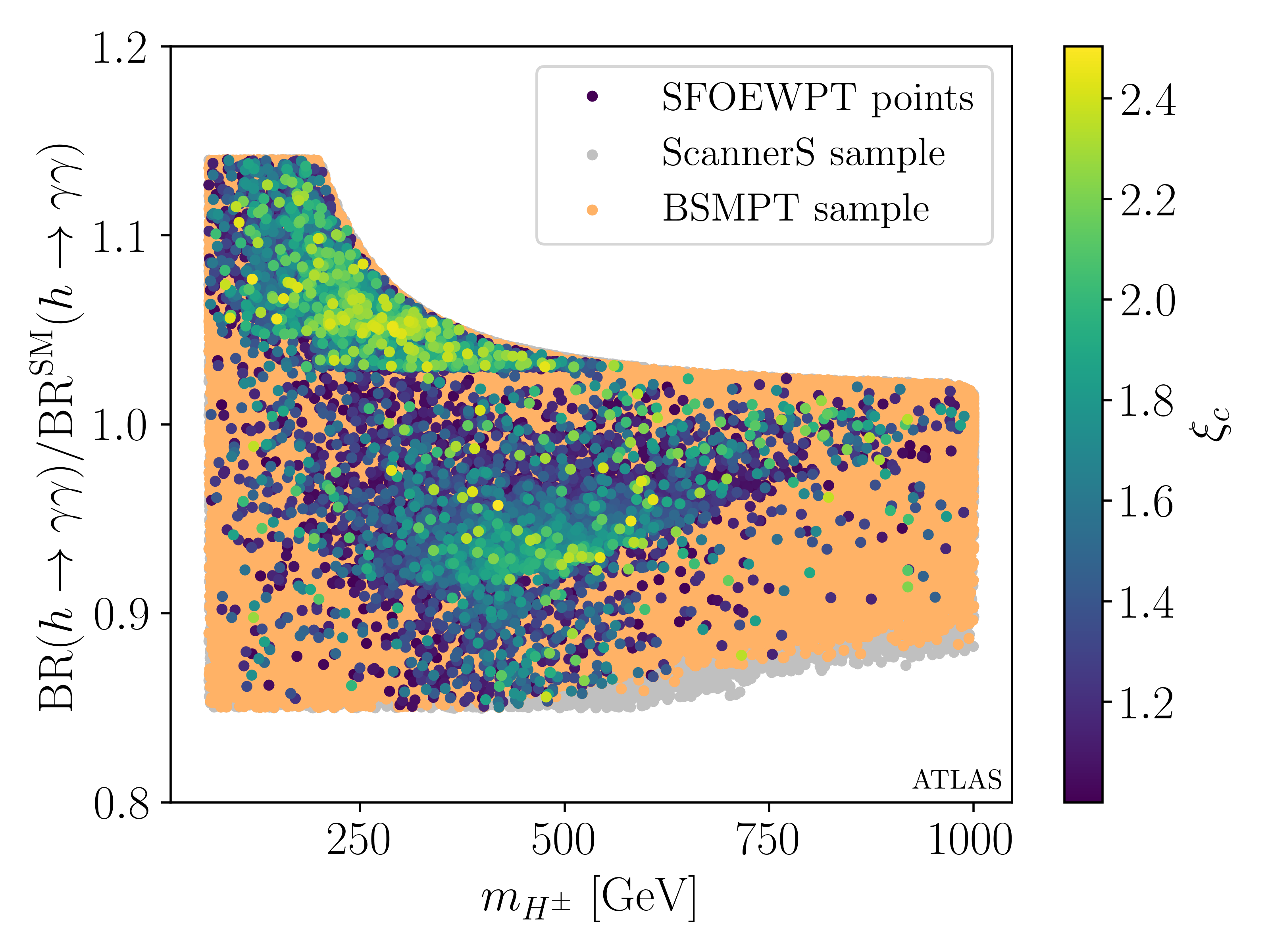
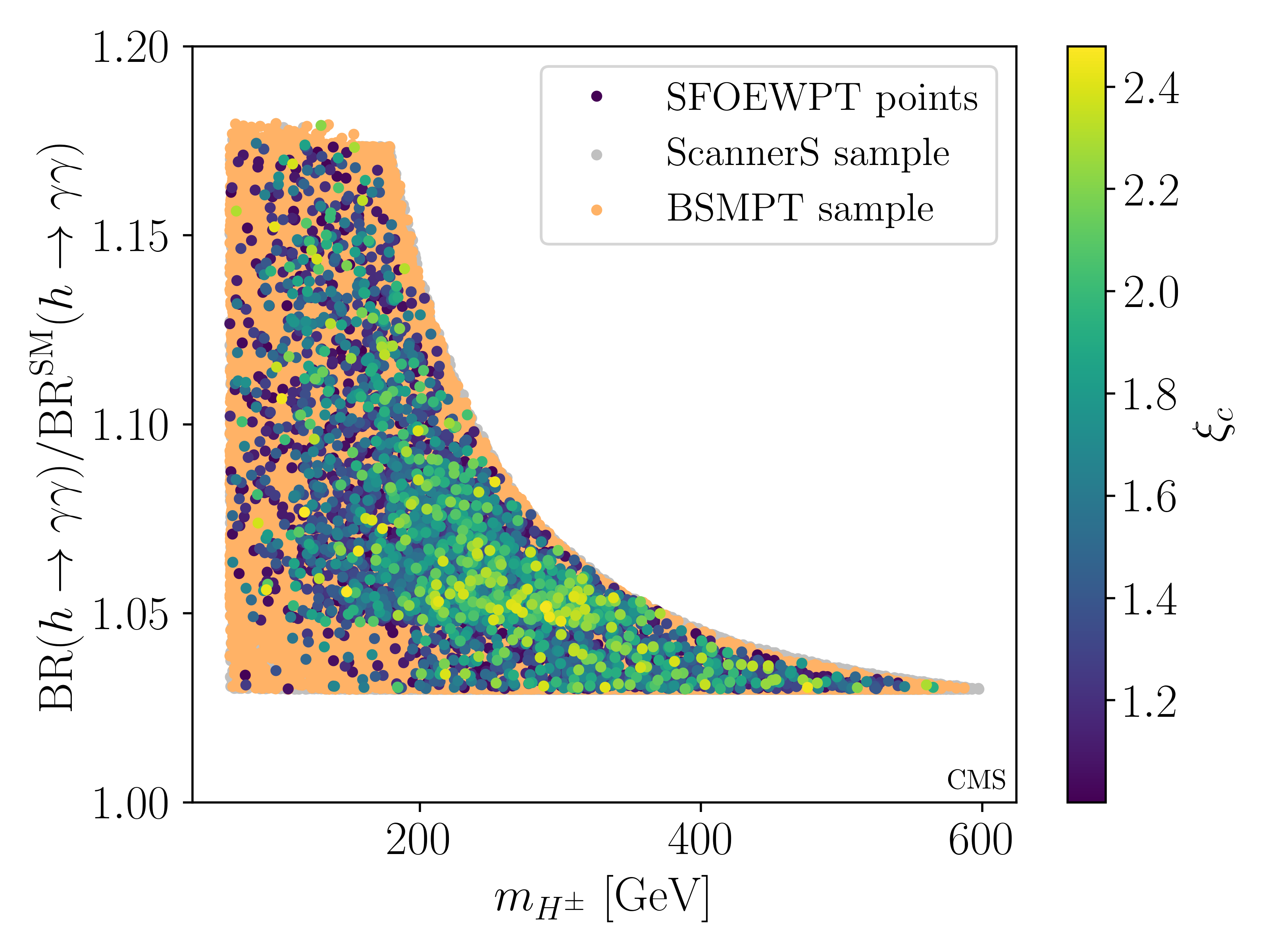
Figure 1: Branching ratio of the SM-like Higgs $h$ into a photon pair normalised to the SM value versus $m_{H^{\pm}}$ applying the ATLAS limit (left) and the CMS limit (right) on $\mu_{\gamma\gamma}$. Gray points: ScannerS sample; orange points: additionally BSMPT constraints imposed; coloured points: also $\xi_{c}>1$ fulfilled. Colour code: value of $\xi_{c}$.

As can be inferred from the plot, the maximum possible branching ratio values increase towards smaller charged Higgs boson masses. Both the value of $m_{H^{\pm}}$ and the $hH^{+}H^{-}$ coupling are governed by $\lambda_{3}$. The value of the branching ratio into $\gamma\gamma$ increases with negative $\lambda_{3}$ and the charged Higgs masses decreases, explaining the behaviour in the plot, cf. also [19] for a detailed discussion. The parameter space of our model is constrained by the experimental limits on the photonic rate, the CMS limit allows for somewhat larger, the ATLAS limit for smaller $\mu_{\gamma\gamma}$. Note, however, that the allowed points are cut below the maximally allowed value by CMS of $\mu_{\gamma\gamma}=1.21$. The upper bound actually results from the combination of the bounded-from-below and unitarity bounds that restrict the allowed values of the coupling $\lambda_{3}$. The plots show that a future increased precision in $\mu_{\gamma\gamma}$ can cut the parameter space on the charged Higgs mass substantially. As can be inferred from the left plot, the charged Higgs mass range starts being cut from $\mu_{\gamma\gamma}$ values above about 1.02 on. In the following plots, we use ScannerS samples that include the more recent limit on $\mu_{\gamma\gamma}$ which is given by CMS. It reduces the upper bound on the allowed charged Higgs mass to 597 GeV. The inclusion of the BSMPT constraints reduce it further to 587 GeV, and the requirement of an SFOEWPT to 565 GeV finally. The reduction in $m_{H^{\pm}}$ in turn also reduces the range of allowed dark neutral masses as we will see.

As for the parameter points with an SFOEWPT, they are distributed nearly all over the still allowed parameter space. The demand of an SFOEWPT hence does not significantly constrain our model with respect to the Higgs data. While the SFOEWPT limit on $m_{H^{\pm}}$ is somewhat below the BSMPT limit, a dedicated parameter scan might also provide SFOEWPT values with larger charged Higgs mass values. Vice versa the Higgs rate measurements in photonic final states do not constrain baryogenesis scenarios of ‘CP in the Dark’.

In Fig. 2 (left) we display the branching ratios of the SM-like Higgs boson $h$ into invisible particles versus the DM mass $m_{h_{1}}$ and in Fig. 2 (right) versus the gauge boson signal strength $\mu_{VV}$ ($V=Z,W$). As mentioned above, we have applied here and in all other plots presented in the numerical analysis the additional cut on $\text{BR}(h\rightarrow\,\text{inv.})<$0.11$$ following the latest results of [56]. We find viable parameter points down to DM masses of about $m_{h_{1}}=54.8$ GeV. Below this value it becomes increasingly difficult to find parameter points that comply with all considered constraints. The parameter points compatible with an SFOEWPT are scattered across the still allowed ScannerS region. Therefore, future improved measurements of $h\rightarrow\text{inv.}$ are able to test the parameter space of ‘CP in the Dark’ but they will not give us additional information on the strength of the phase transition itself. Above $m_{h_{1}}=62.5$ GeV (not shown in the plot) the branching ratio of course drops to zero as the corresponding decay is kinematically closed.

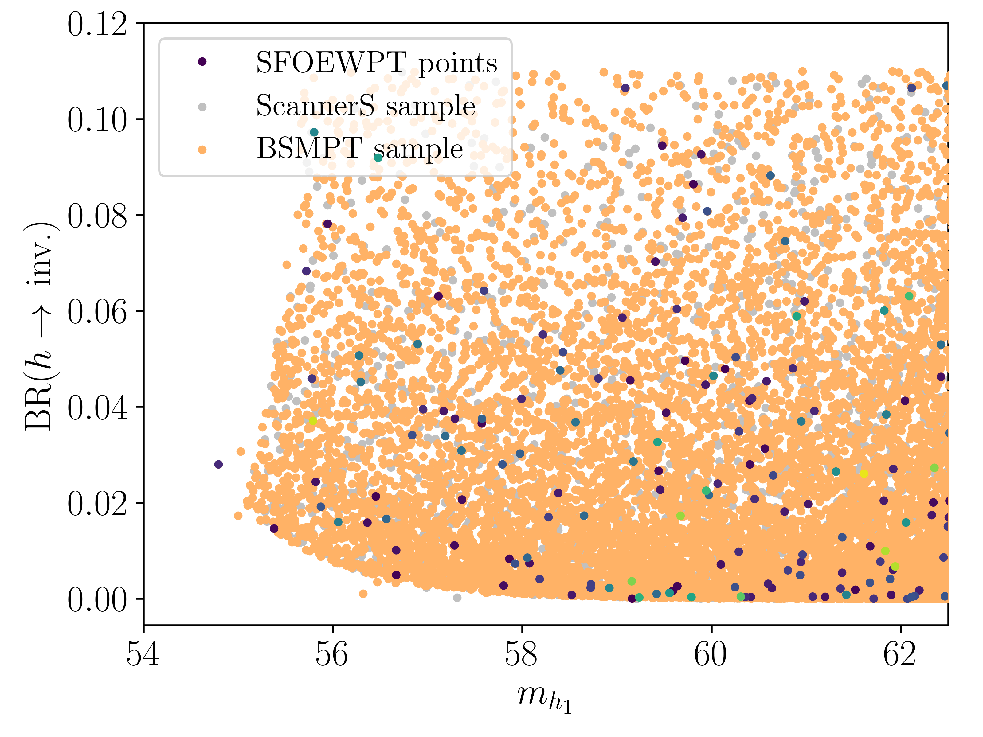
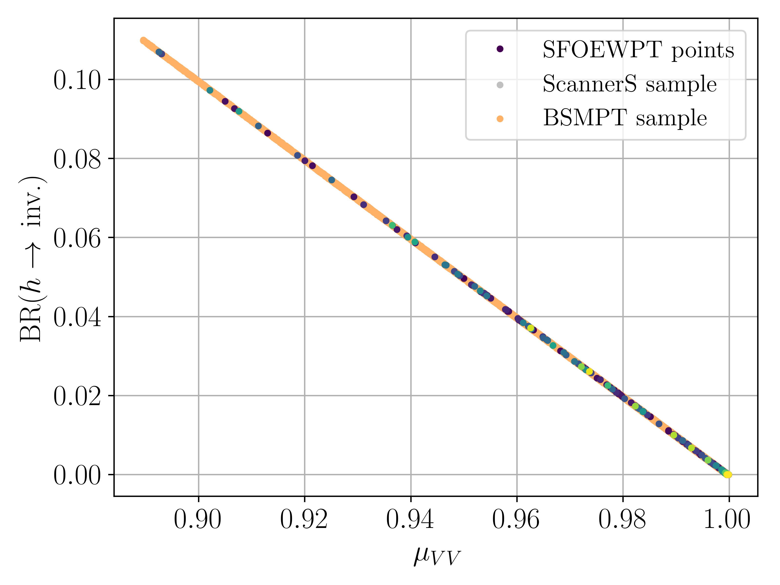
Figure 2: Branching ratio of the SM-like Higgs $h$ into dark particles versus $m_{h_{1}}$ (left) and versus $\mu_{VV}$ (right). The colour code is the same as in Fig. 1.

The results for $\text{BR}(h\rightarrow\,\text{inv.})$ versus $\mu_{VV}$ in Fig. 2 (right) look similar to those found in [70] for the fully dark phase (FDP) of the N2HDM which is very similar to our model. Since all tree-level $h$ couplings are SM-like the invisible branching ratio strongly correlates with $\mu_{VV}$. It decreases for increasing $\mu_{VV}$ until $\text{BR}(h\rightarrow\,\text{inv.})=0$ when $\mu_{VV}=1$. This is expected as for $\mu_{VV}\rightarrow 1$, the SM-like Higgs branching ratios converge to their SM values with no decays into invisible particles being allowed. Future precise measurements of the $\mu_{VV}$ rates will hence constrain the invisible branching ratios and thereby the parameter space of the model, but again not give further insights on the strength of the EWPT as can be inferred from the distribution of the coloured points.

5.2 Mass Parameter Distributions for an SFOEWPT

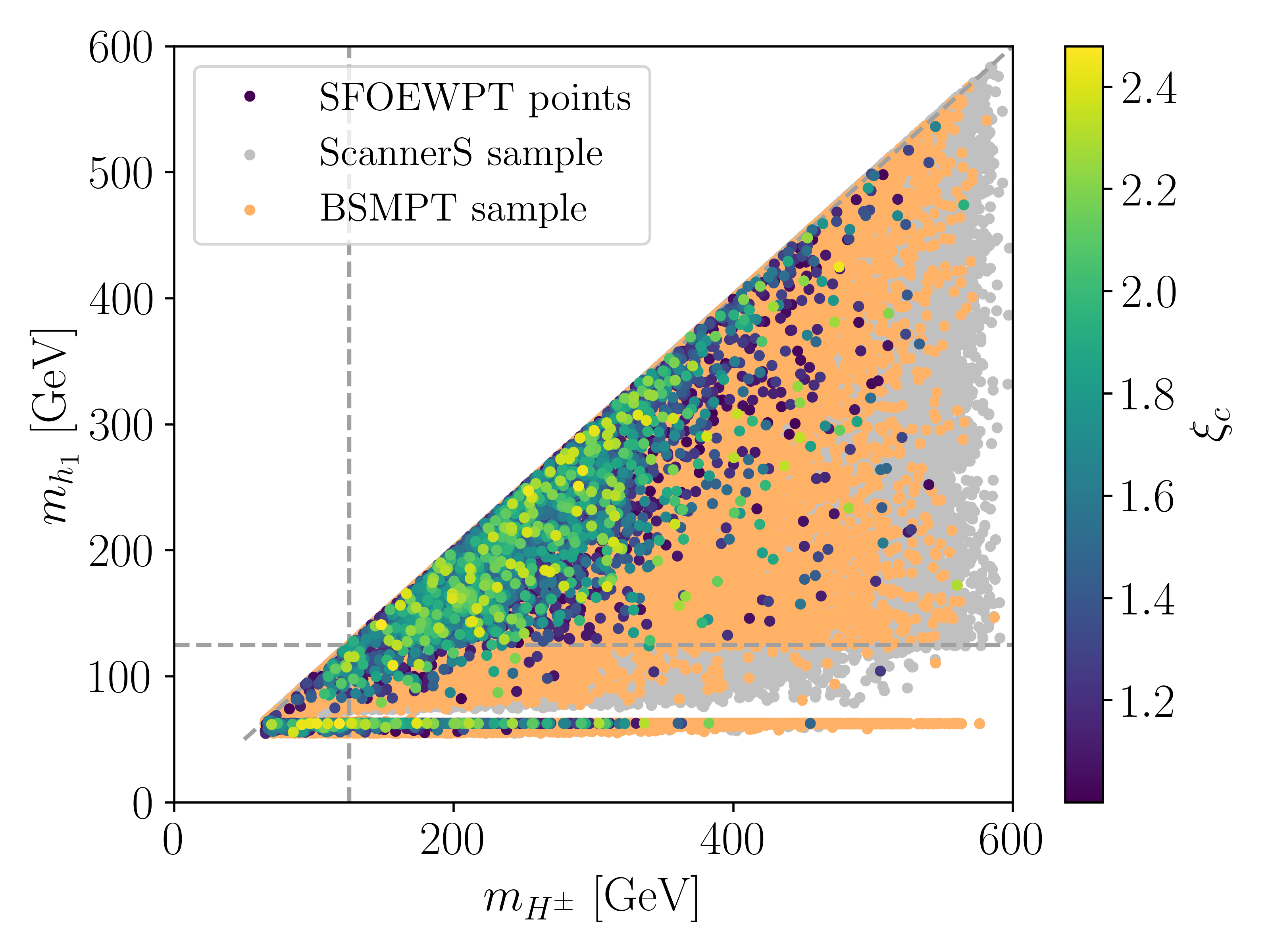
Figure 3: Scatter plot in the $m_{h_{1}}$ and $m_{H^{\pm}}$ mass plane. The dashed lines are there to guide the eye and denote the $m_{h_{1}}$ and $m_{H^{\pm}}$ values at 125 GeV and the points where their masses are equal. Colour code as in Fig. 1.

Figure 3 shows for the parameter points of our scan the lightest neutral dark scalar mass $m_{h_{1}}$ versus the dark charged scalar mass $m_{H^{\pm}}$. The colour code is the same as in the previous figures. The constraint on the charged Higgs mass values from $\mu_{\gamma\gamma}$ also constrains the allowed $m_{h_{1}}$ values which can go up to 584 GeV in the ScannerS sample, to 568 GeV after inclusion of the BSMPT constraints, and reaches a maximum value of 536 GeV for points providing an SFOEWPT. Depending on the future restriction on $\mu_{\gamma\gamma}$ the charged Higgs mass will be less or more constrained with immediate consequences for the allowed range of $m_{h_{1}}$. The points with $\xi_{c}\geq 1$ cluster towards smaller mass values. We still find SFOEWPT points for larger masses, however. A dedicated scan in this mass region may increase their density. So again, the requirement of an SFOEWPT does not significantly constrain the parameter space nor do the Higgs constraints further restrict the points leading to $\xi_{c}$ values above 1. We note that the distribution structure of the points stems from the fact that we performed a dedicated scan in the $m_{h_{1}}$ mass region below 125/2 GeV resulting in the horizontally distributed points in the region below 62.5 GeV.

In Fig. 4 we display the distribution of our parameter point sample in the neutral DM mass planes, namely $m_{h_{1}}$ versus $m_{h_{2}}$ (left) and $m_{h_{1}}$ versus $m_{h_{3}}$ (right). Again the restricted $m_{H^{\pm}}$ range is reflected in the allowed upper values of the dark neutral masses. In the $m_{h_{1}}-m_{h_{3}}$ plane we see a tendency of SFOEWPT points to cluster towards smaller mass values. Still we have also points for larger values in the allowed BSMPT sample. The requirement of an SFOEWPT does not allow us to read off strict bounds on the mass values.

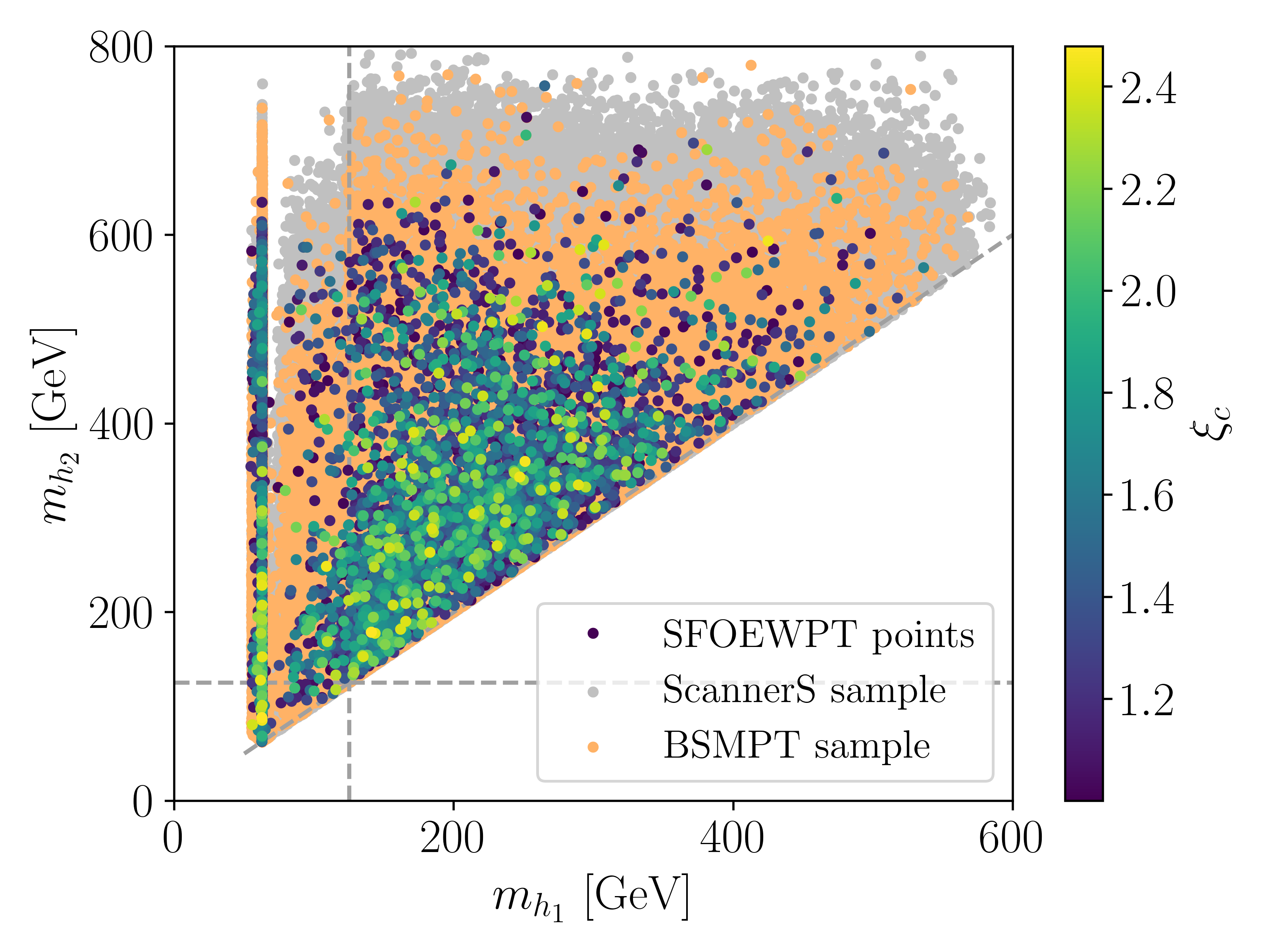
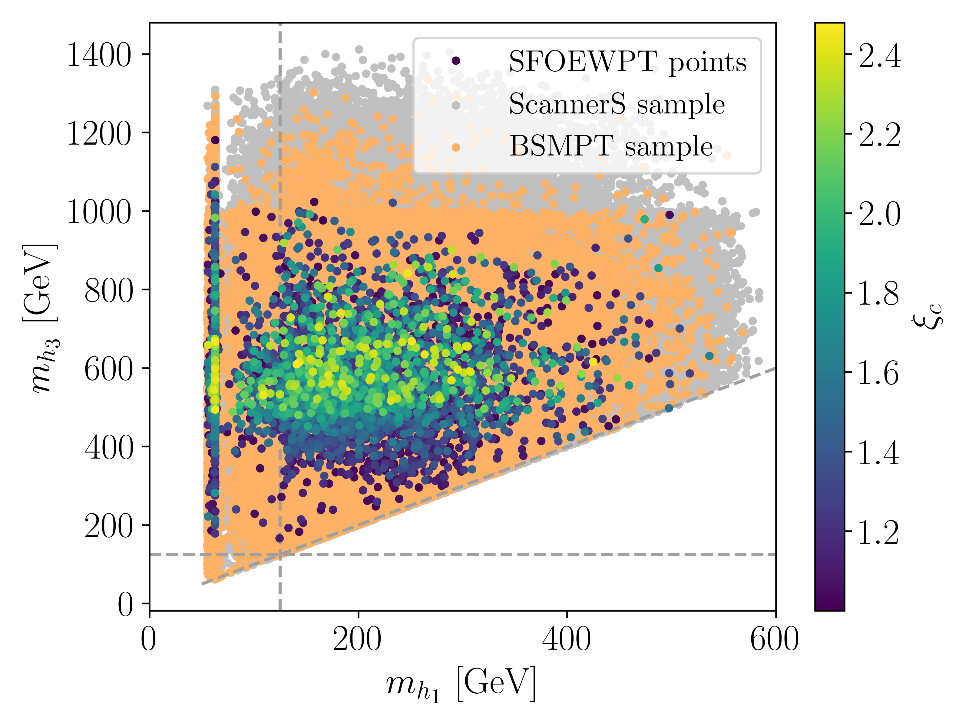
Figure 4: Scatter plot $m_{h_{1}}$ versus $m_{h_{2}}$ (left) and $m_{h_{1}}$ versus $m_{h_{3}}$ (right). The dashed lines are there to guide the eye and denote neutral dark mass values at 125 GeV and the points where their masses in the respective plane are equal. The colours denote the same constraints as in Fig. 1.

5.3 Analysis of the VEV Configurations

In all our allowed parameter samples we find that the charge-breaking VEV is zero as required for the photon to remain massless. As for the other VEVs, at non-zero temperature we find two VEV patterns: In one, the SM-like VEV is non-zero while the remaining DM VEVs are negligibly small. This is the case for almost all allowed parameters sets. The other case is given by a very small fraction of allowed parameter points. Here we find VEV configurations where also the dark VEVs develop non-zero values.

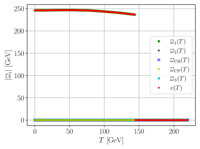
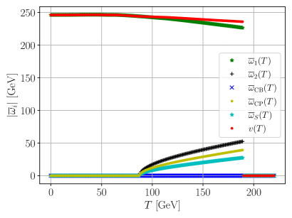
Figure 5: Evolution of the VEVs as a function of $T$ for a point where only $|\overline{\omega}_{1}|\neq 0$ (left) and for a point where all except the charge-breaking VEV are non-zero at $T_{c}$. The temperature-dependent electroweak VEV $v(T)$ is defined in Eq. (3.24) and shown in red. Both benchmark points are given in App. A.

In Fig. 5 we illustrate the evolution of all five VEVs as a function of the temperature for two sample points, one for each of the two categories. The sample points are given in App. A. In red, we display the temperature-dependent electroweak VEV $v(T)$, that is calculated taking into account the $SU(2)_{L}$-VEVs, see Eq. (3.24). Both points displayed in Fig. 5 show a discontinuity in $v_{c}(T)$ at $T=T_{c}$ that is large enough to be classified as SFOEWPT. Actually, we have $\xi_{c}=1.64$ for the left and $\xi_{c}=1.24$ for the right scenario. Only for the scenario depicted in the right plot, however, also dark VEVs participate in the SFOEWPT in addition to $|\overline{\omega}_{1}|$ which is non-zero for all $T<T_{c}$. The development of a non-zero CP-violating VEV $|\overline{\omega}_{\text{CP}}|$ (which remains non-zero down to $T=88$ GeV $<T_{c}$ and is zero at zero temperature) actually corresponds to the generation of spontaneous CP violation.

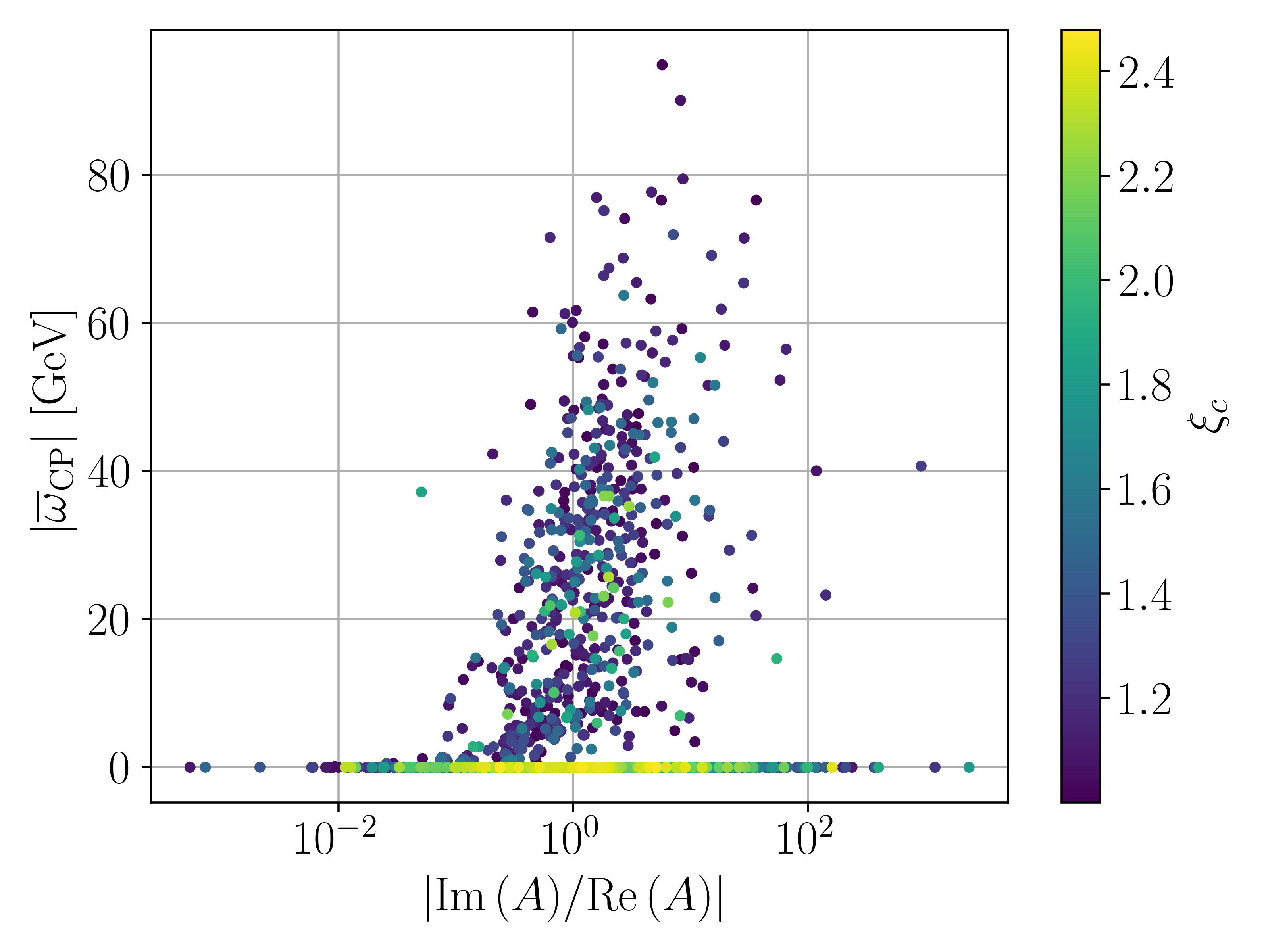
Figure 6: The CP-violating VEV $\overline{\omega}_{\text{CP}}$ versus $|\operatorname{Im}(A)/\operatorname{Re}(A)|$ for all SFOEWPT points. The colour code indicates the strength $\xi_{c}>1$ of the SFOEWPT.

In Fig. 6 we show the absolute value of the CP-violating VEV $\overline{\omega}_{\text{CP}}$ as a function of the absolute value of the ratio $\operatorname{Im}(A)$ over $\operatorname{Re}(A)$ for all allowed SFOEWPT points of our scan. As discussed in Sec. 2, a non-zero imaginary part of the trilinear coupling $A$ induces explicit CP violation. At $T=0$ GeV, CP violation can only be generated explicitly, as $\overline{\omega}_{\text{CP}}\big{|}_{T=$0\text{\,}\mathrm{G}\mathrm{e}\mathrm{V}$}\equiv v_{\text{CP}}=0$. We find in total 564 points for which $|\overline{\omega}_{\text{CP}}|\neq 0$ (more specifically, $|\overline{\omega}_{\text{CP}}|>0.001$ GeV) at finite temperature and which hence break CP spontaneously at $T>0$. Additionally, these points develop a non-vanishing singlet VEV $\overline{\omega}_{S}$ at $T\neq 0$. This means that also the $\mathbb{Z}_{2}$-symmetry is spontaneously broken. At finite temperature, the dark charge therefore is not conserved, and particles that are dark at zero temperature can now mix with particles from the first doublet. This is very interesting as it provides a promising portal for the transfer of non-standard CP violation to the SM-like Higgs couplings to fermions at finite temperature. This is in addition to an SFOEWPT another necessary ingredient for an EWBG scenario that is able to explain today’s observed BAU. We finally note, that the plot does not show a clear correlation between the size of $|\overline{\omega}_{\text{CP}}|$ and $\operatorname{Im}(A)\neq 0$. However, we see that $|\overline{\omega}_{\text{CP}}|>0$ only for $\operatorname{Im}(A)\neq 0$. From the plot we cannot deduce a correlation between the size of $\xi_{c}$ and $|\overline{\omega}_{\text{CP}}|$: For the strength of the phase transition, overall the participation of additional Higgs bosons and their involved mass values is decisive. It is not important which kind of VEV contributes to $v_{c}(T)$.

5.4 Dark Matter Observables

In Fig. 7 we show our benchmark point sample in the plane spanned by the relic density $\Omega h^{2}$, calculated via ScannerS through the link with MicrOMEGAs, and the mass of the DM candidate, $m_{h_{1}}$. The experimentally measured relic density $\Omega_{\text{obs}}h^{2}=$0.1200(12)$$ [67] is shown in red. The colour code is the same as in Fig. 1. While we find ScannerS sample points that lie within the $1\sigma$ error bands for the measured relic density, the SFOEWPT points are all underabundant. Parameter samples with masses around $m_{h_{1}}/2$ can be less underabundant than scenarios with heavier DM particles. The underabundance is not problematic. It simply means that we need another DM component to make up for the total of the relic density. We can hence state that the requirement of an SFOEWPT in ‘CP in the Dark’ is compatible with the measured DM relic density.

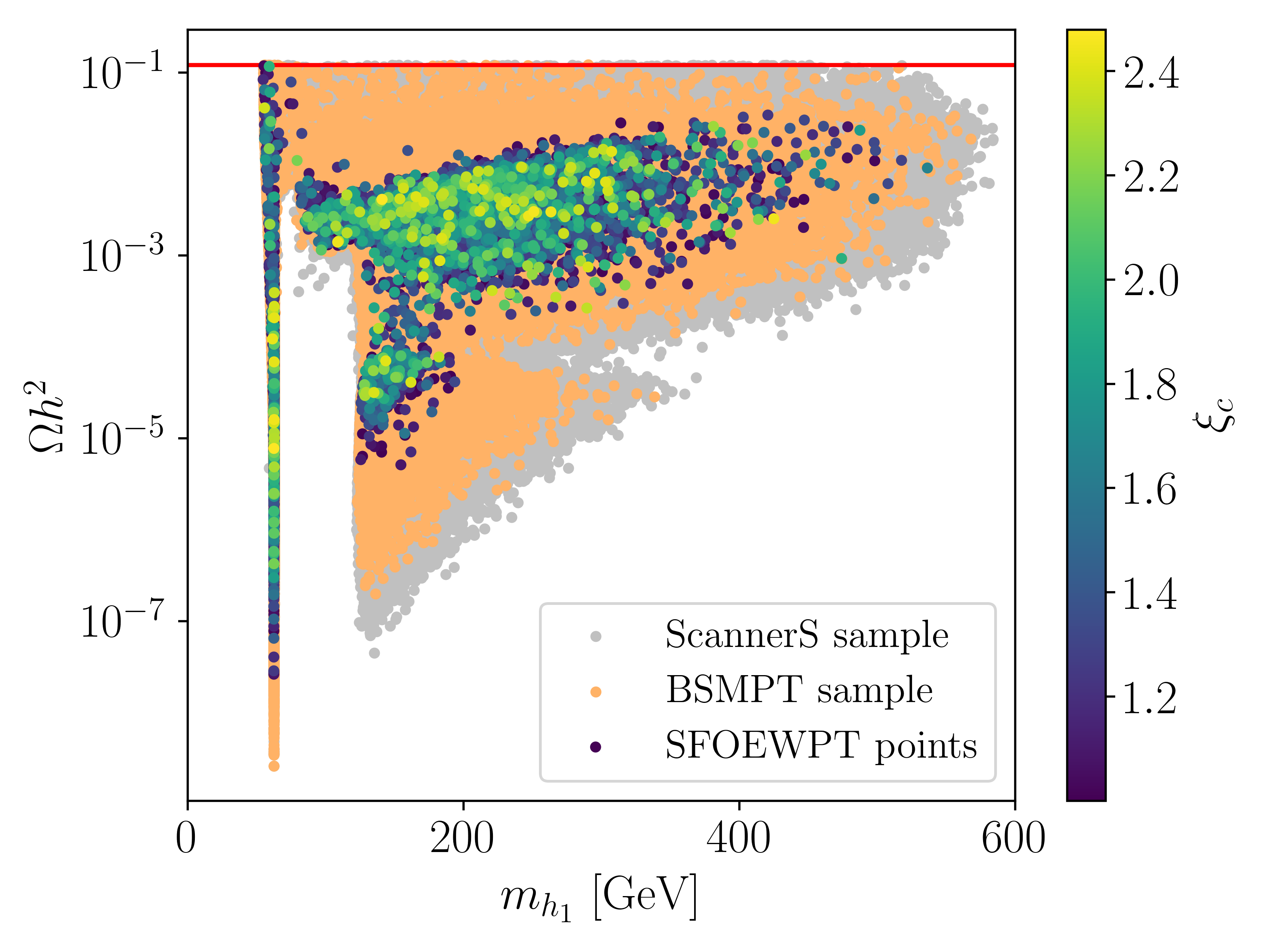
Figure 7: Relic density versus DM mass $m_{h_{1}}$ for the benchmark parameter sample, with the colour code introduced in Fig. 1. The experimentally measured relic density $\Omega_{\text{obs}}h^{2}=$0.1200(12)$$ [67] is shown in red.

In order to investigate the impact of the measurements of the direct detection spin-independent (SI) nucleon DM cross section $\sigma$ we first compute the effective cross section $f_{\chi\chi}\cdot\sigma$ for our model,

$$\sigma\cdot f_{\chi\chi}\equiv\sigma\cdot\frac{\Omega_{\text{prod}}h^{2}}{\Omega_{\text{obs}}h^{2}}\,.$$ (5.40)

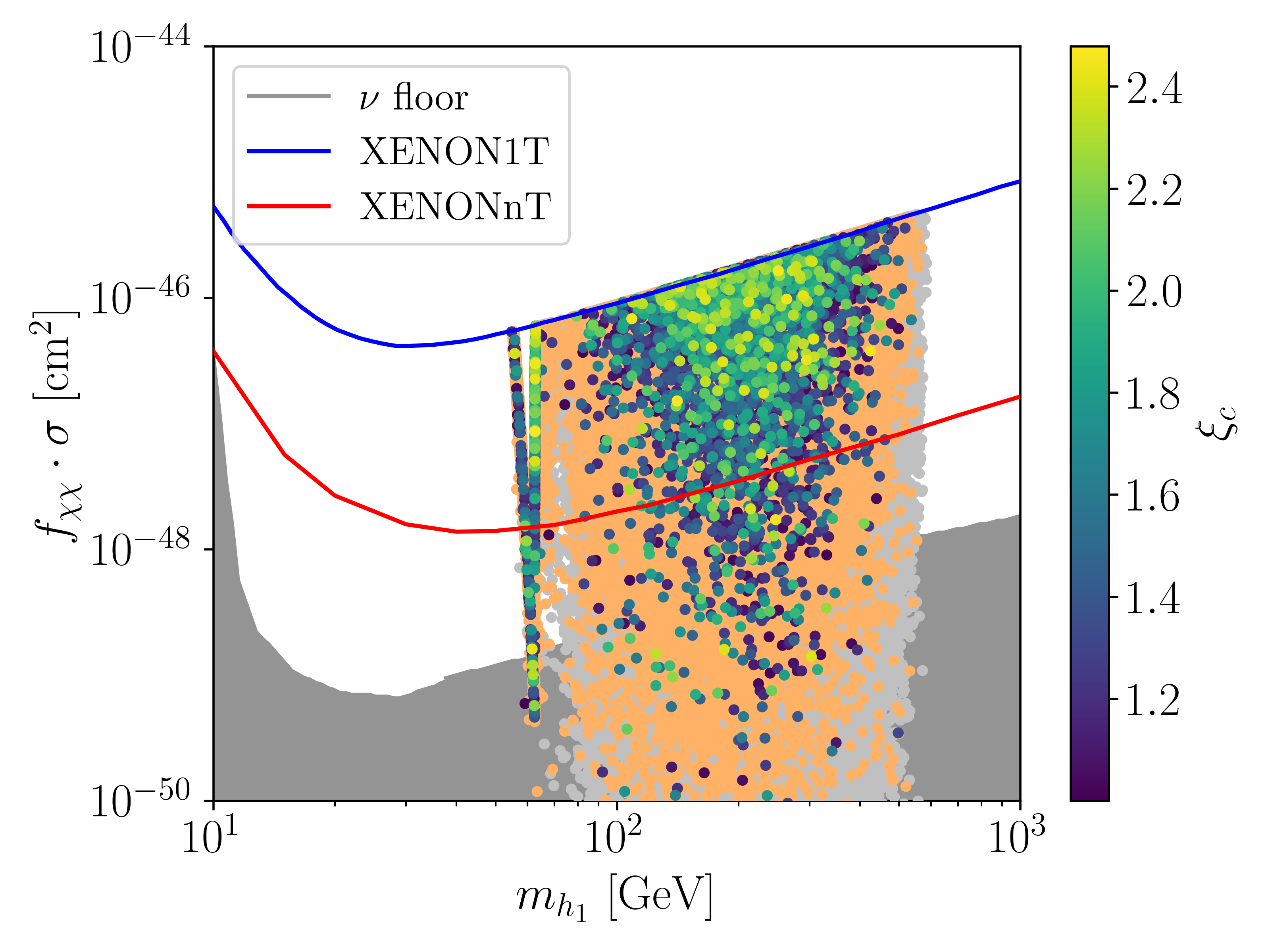
Figure 8: Effective direct detection SI nucleon DM cross section of the benchmark point sample versus $m_{h_{1}}$, with the colour code defined as in Fig. 1. The experimental results have been obtained by using [71]. The XENON1T exclusion limit [72] is shown in blue. In red, we show the projected sensitivity of the XENONnT experiment [73]. The experimental limit for the neutrino background has been taken from [74].

The rescaling factor $f_{\chi\chi}$ considers the fact that in our model, depending on the parameter point, the relic density $\Omega_{\text{prod}}h^{2}$ can be underabundant, which has to be taken into account when comparing with the measured value of $\sigma$, cf. also [70, 75]. The numerical values for the produced relic density $\Omega_{\text{prod}}h^{2}$ in our model are obtained using MicrOMEGAs. In Fig. 8 we display the effective direct detection SI nucleon DM cross section $f_{\chi\chi}\cdot\sigma$ of the benchmark point sample versus $m_{h_{1}}$. As already required by the constraints in ScannerS (linked to MicrOMEGAs), all points lie below the XENON1T exclusion limit, which is displayed in blue. The majority of the SFOEWPT points is found to be above the neutrino floor (dark grey shaded area). In addition, most SFOEWPT points are also above the expected sensitivity of the XENONnT experiment (red). This means that future DM direct detection experiments will allow us to test a large fraction of the parameter space of ‘CP in the Dark’ that is compatible with an SFOEWPT.

6 Conclusion

In this paper, we investigated the possibility of an SFOEWPT within the framework of the model ‘CP in the Dark’. Its extended N2HDM-like scalar sector provides a dark sector that is stabilised at zero temperature through only one $\mathbb{Z}_{2}$ symmetry and thereby provides a DM candidate. We discussed the treatment of finite pieces of our renormalisation scheme and the necessary adjustments for this model in contrast to past work to be able to renormalise the one-loop mixing angles and masses to their leading-order values. This allows us to efficiently perform parameter scans taking into account the relevant theoretical and experimental constraints to obtain viable parameter sets. The new BSMPT version v2.3 including the implementation of ‘CP in the Dark’ has been made publicly available under https://github.com/phbasler/BSMPT.

Our results show that ‘CP in the Dark’ proves itself to be a highly promising candidate to explain the BAU in an EWBG context, as in addition to explicit CP violation in the dark sector, it also provides spontaneous CP violation at finite temperature. In combination with the also spontaneously broken $\mathbb{Z}_{2}$ symmetry at non-zero temperature non-standard CP violation can be transferred to the couplings of the SM-like Higgs boson to fermions. This may allow for a large enough CP violation to generate the BAU observed by experiment, without being in conflict with the EDM constraints.

Viable SFOEWPT points are distributed across almost the whole allowed dark mass ranges of the model. While the SM-like Higgs rates will allow us to constrain the parameter space of the model, the SFOEWPT points do not impose further significant constraints. On the other hand, SFOEWPT points are found to be in the reach of precise measurements of invisible decays of the SM-like Higgs boson and of the Higgs rates into SM particles at the LHC. Our SFOEWPT points comply with the measured relic density. We found that a large fraction of the parameter space and SFOEWPT points of the model will be testable at future DM direct detection experiments.

Having demonstrated in this paper that all prerequisites for BAU are fulfilled in the model, the next natural steps to be taken in future work is the implementation of the computation of the amount of baryogenesis in BSMPT in order to investigate if the model can indeed provide the correct amount of BAU. If this is the case, subsequently LHC and DM observables are to be identified that may serve as smoking gun signatures for parameter scenarios compatible with BAU in ‘CP in the Dark’.

Acknowledgments

The research of MM was supported by the Deutsche Forschungsgemeinschaft (DFG, German Research Foundation) under grant 396021762 - TRR 257. JM acknowledges support by the BMBF-Project 05H18VKCC1. We thank Philipp Basler, Duarte Azevedo, Günter Quast, Jonas Wittbrodt and Michael Spira for fruitful discussions.

Appendix A Benchmark Points

The input values of the benchmark points discussed in Subsec. 5.3 are given in Tab. 2. The dark mass values, critical temperature, critical VEV, $\xi_{c}$ and the individual VEVs at $T_{c}$ are given in Tab. 3. Note that we have $\lambda_{1}\simeq$0.258$$, $m_{11}^{2}\simeq$-7824$$ GeV² for both points. The parameter $\lambda_{1}$ is fixed through $m_{h}^{2}=\lambda_{1}v_{1}^{2}$ and the value for $m_{11}^{2}$ follows from the minimisation condition.

point	$m_{22}^{2}\,[$\mathrm{G}\mathrm{e}\mathrm{V}$^{2}]$	$m_{S}^{2}\,[$\mathrm{G}\mathrm{e}\mathrm{V}$^{2}]$	$\text{Re}\,(A)\,[$\mathrm{G}\mathrm{e}\mathrm{V}$]$	$\text{Im}\,(A)\,[$\mathrm{G}\mathrm{e}\mathrm{V}$]$	$\lambda_{1}$
Fig. 5(a)	$96\,703.414$	$32\,442.949$	$159.627$	$-325.391$	$3.532$
Fig. 5(b)	$65\,258.809$	$36\,279.847$	$279.502$	$-326.645$	$3.660$
point	$\lambda_{3}$	$\lambda_{4}$	$\lambda_{5}$	$\lambda_{6}$	$\lambda_{7}$	$\lambda_{8}$
Fig. 5(a)	$-0.796$	$0.787$	$-0.055$	$10.446$	$7.596$	$4.683$
Fig. 5(b)	$-0.821$	$0.220$	$-0.371$	$4.715$	$7.760$	$14.781$

Table 2: Input parameters of the two benchmark points of Fig. 5. We set $v_{1}\equiv v\approx 246.22$ GeV and $m_{h}=125.09$ GeV.

point	$m_{H^{\pm}}$	$m_{h_{1}}$	$m_{h_{2}}$	$m_{h_{3}}$	$T_{c}$	$v_{c}$
Fig. 5(a)	$269.386$	$241.718$	$308.943$	$549.265$	$144.21$	$236.53$
Fig. 5(b)	$200.940$	$62.680$	$218.700$	$560.206$	$189.77$	$235.85$
point	$\xi_{c}$	$\overline{\omega}_{\text{CB}}$	$\overline{\omega}_{1}$	$\overline{\omega}_{2}$	$\overline{\omega}_{\text{CP}}$	$\overline{\omega}_{S}$
Fig. 5(a)	$1.64$	$-8.977\text{\times}{10}^{-07}$	$236.53$	$9.093\text{\times}{10}^{-07}$	$-3.793\text{\times}{10}^{-07}$	$4.604\text{\times}{10}^{-07}$
Fig. 5(b)	$1.24$	$-2.212\text{\times}{10}^{-05}$	$226.46$	$52.72$	$39.52$	$-27.58$

Table 3: Dark mass values, critical temperature and critical VEV, $\xi_{c}$, and individual VEVs at $T_{c}$ of the two benchmark points of Fig. 5. All values, except for $\xi_{c}$, are given in GeV.

References

- [1] ATLAS, G. Aad et al., Phys. Lett. B716, 1 (2012), 1207.7214.
- [2] CMS, S. Chatrchyan et al., Phys. Lett. B716, 30 (2012), 1207.7235.
- [3] WMAP, C. L. Bennett et al., Astrophys. J. Suppl. 208, 20 (2013), 1212.5225.
- [4] V. A. Kuzmin, V. A. Rubakov, and M. E. Shaposhnikov, Phys. Lett. 155B, 36 (1985).
- [5] A. G. Cohen, D. B. Kaplan, and A. E. Nelson, Nucl. Phys. B349, 727 (1991).
- [6] A. G. Cohen, D. B. Kaplan, and A. E. Nelson, Ann. Rev. Nucl. Part. Sci. 43, 27 (1993), hep-ph/9302210.
- [7] M. Quiros, Helv. Phys. Acta 67, 451 (1994).
- [8] V. A. Rubakov and M. E. Shaposhnikov, Usp. Fiz. Nauk 166, 493 (1996), hep-ph/9603208, [Phys. Usp.39,461(1996)].
- [9] K. Funakubo, Prog. Theor. Phys. 96, 475 (1996), hep-ph/9608358.
- [10] M. Trodden, Rev. Mod. Phys. 71, 1463 (1999), hep-ph/9803479.
- [11] W. Bernreuther, Lect. Notes Phys. 591, 237 (2002), hep-ph/0205279, [,237(2002)].
- [12] D. E. Morrissey and M. J. Ramsey-Musolf, New J. Phys. 14, 125003 (2012), 1206.2942.
- [13] A. D. Sakharov, Pisma Zh. Eksp. Teor. Fiz. 5, 32 (1967), [Usp. Fiz. Nauk161,no.5,61(1991)].
- [14] N. S. Manton, Phys. Rev. D28, 2019 (1983).
- [15] F. R. Klinkhamer and N. S. Manton, Phys. Rev. D30, 2212 (1984).
- [16] K. Kajantie, M. Laine, K. Rummukainen, and M. E. Shaposhnikov, Phys. Rev. Lett. 77, 2887 (1996), hep-ph/9605288.
- [17] F. Csikor, Z. Fodor, and J. Heitger, Phys. Rev. Lett. 82, 21 (1999), hep-ph/9809291.
- [18] M. B. Gavela, P. Hernandez, J. Orloff, and O. Pene, Mod. Phys. Lett. A 9, 795 (1994), hep-ph/9312215.
- [19] D. Azevedo et al., JHEP 11, 091 (2018), 1807.10322.
- [20] T. D. Lee, Phys. Rev. D8, 1226 (1973).
- [21] G. C. Branco et al., Phys. Rept. 516, 1 (2012), 1106.0034.
- [22] M. Muhlleitner, M. O. P. Sampaio, R. Santos, and J. Wittbrodt, JHEP 03, 094 (2017), 1612.01309.
- [23] A. Cordero-Cid et al., JHEP 12, 014 (2016), 1608.01673.
- [24] D. Sokołowska, J. Phys. Conf. Ser. 873, 012030 (2017).
- [25] C.-Y. Chen, M. Freid, and M. Sher, Phys. Rev. D89, 075009 (2014), 1312.3949.
- [26] I. Engeln, M. Mühlleitner, and J. Wittbrodt, Comput. Phys. Commun. 234, 256 (2019), 1805.00966.
- [27] R. Coimbra, M. O. P. Sampaio, and R. Santos, Eur. Phys. J. C73, 2428 (2013), 1301.2599.
- [28] P. M. Ferreira, R. Guedes, M. O. P. Sampaio, and R. Santos, JHEP 12, 067 (2014), 1409.6723.
- [29] M. Mühlleitner, M. O. Sampaio, R. Santos, and J. Wittbrodt, (2020), 2007.02985.
- [30] P. Basler and M. Mühlleitner, Comput. Phys. Commun. 237, 62 (2019), 1803.02846.
- [31] P. Basler, M. Mühlleitner, and J. Müller, Comput. Phys. Commun. 269, 108124 (2021), 2007.01725.
- [32] P. Basler, M. Krause, M. Muhlleitner, J. Wittbrodt, and A. Wlotzka, JHEP 02, 121 (2017), 1612.04086.
- [33] P. Basler, M. Mühlleitner, and J. Wittbrodt, JHEP 03, 061 (2018), 1711.04097.
- [34] P. Basler, M. Mühlleitner, and J. Müller, JHEP 05, 016 (2020), 1912.10477.
- [35] G. D. Moore, Phys. Rev. D59, 014503 (1999), hep-ph/9805264.
- [36] L. Dolan and R. Jackiw, Phys. Rev. D9, 3320 (1974).
- [37] H. H. Patel and M. J. Ramsey-Musolf, JHEP 07, 029 (2011), 1101.4665.
- [38] C. Wainwright, S. Profumo, and M. J. Ramsey-Musolf, Phys. Rev. D84, 023521 (2011), 1104.5487.
- [39] M. Garny and T. Konstandin, JHEP 07, 189 (2012), 1205.3392.
- [40] P. Basler, M. Mühlleitner, and J. Müller, (2021), 2108.03580.
- [41] ATLAS, CMS, G. Aad et al., Phys. Rev. Lett. 114, 191803 (2015), 1503.07589.
- [42] Particle Data Group, K. A. Olive et al., Chin. Phys. C38, 090001 (2014).
- [43] L. H. C. S. W. Group, 2016.
- [44] LHC Higgs Cross Section Working Group, S. Dittmaier et al., (2011), 1101.0593.
- [45] L.-L. Chau and W.-Y. Keung, Phys. Rev. Lett. 53, 1802 (1984).
- [46] I. P. Ivanov and J. P. Silva, Phys. Rev. D92, 055017 (2015), 1507.05100.
- [47] P. Bechtle, O. Brein, S. Heinemeyer, G. Weiglein, and K. E. Williams, Comput. Phys. Commun. 181, 138 (2010), 0811.4169.
- [48] P. Bechtle, O. Brein, S. Heinemeyer, G. Weiglein, and K. E. Williams, Comput. Phys. Commun. 182, 2605 (2011), 1102.1898.
- [49] P. Bechtle et al., PoS CHARGED2012, 024 (2012), 1301.2345.
- [50] P. Bechtle et al., Eur. Phys. J. C74, 2693 (2014), 1311.0055.
- [51] P. Bechtle, S. Heinemeyer, O. Stal, T. Stefaniak, and G. Weiglein, Eur. Phys. J. C 75, 421 (2015), 1507.06706.
- [52] P. Bechtle et al., Eur. Phys. J. C 80, 1211 (2020), 2006.06007.
- [53] P. Bechtle, S. Heinemeyer, O. Stål, T. Stefaniak, and G. Weiglein, Eur. Phys. J. C74, 2711 (2014), 1305.1933.
- [54] P. Bechtle, S. Heinemeyer, O. Stål, T. Stefaniak, and G. Weiglein, JHEP 11, 039 (2014), 1403.1582.
- [55] CMS, A. M. Sirunyan et al., JHEP 07, 027 (2021), 2103.06956.
- [56] ATLAS, (2020).
- [57] G. Belanger, F. Boudjema, A. Pukhov, and A. Semenov, Comput. Phys. Commun. 176, 367 (2007), hep-ph/0607059.
- [58] G. Belanger, F. Boudjema, A. Pukhov, and A. Semenov, Comput. Phys. Commun. 180, 747 (2009), 0803.2360.
- [59] G. Belanger et al., Comput. Phys. Commun. 182, 842 (2011), 1004.1092.
- [60] G. Belanger, F. Boudjema, A. Pukhov, and A. Semenov, Nuovo Cim. C 033N2, 111 (2010), 1005.4133.
- [61] G. Belanger, F. Boudjema, A. Pukhov, and A. Semenov, Comput. Phys. Commun. 185, 960 (2014), 1305.0237.
- [62] G. Bélanger, F. Boudjema, A. Pukhov, and A. Semenov, Comput. Phys. Commun. 192, 322 (2015), 1407.6129.
- [63] D. Barducci et al., Comput. Phys. Commun. 222, 327 (2018), 1606.03834.
- [64] G. Bélanger, F. Boudjema, A. Goudelis, A. Pukhov, and B. Zaldivar, Comput. Phys. Commun. 231, 173 (2018), 1801.03509.
- [65] G. Belanger, A. Mjallal, and A. Pukhov, Eur. Phys. J. C 81, 239 (2021), 2003.08621.
- [66] Micromegas, https://lapth.cnrs.fr/micromegas/, Accessed: 2021-07-09.
- [67] Planck, N. Aghanim et al., Astron. Astrophys. 641, A6 (2020), 1807.06209.
- [68] ACME, V. Andreev et al., Nature 562, 355 (2018).
- [69] ATLAS, M. Aaboud et al., Phys. Rev. D 98, 052005 (2018), 1802.04146.
- [70] I. Engeln, P. Ferreira, M. M. Mühlleitner, R. Santos, and J. Wittbrodt, JHEP 08, 085 (2020), 2004.05382.
- [71] A. Desai and A. Moskowitz, DMTOOLS, Dark Matter Limit Plot Generator, Accessed: 2021-07-31.
- [72] XENON, E. Aprile et al., Phys. Rev. Lett. 121, 111302 (2018), 1805.12562.
- [73] XENON, E. Aprile et al., JCAP 11, 031 (2020), 2007.08796.
- [74] J. Billard, L. Strigari, and E. Figueroa-Feliciano, Phys. Rev. D 89, 023524 (2014), 1307.5458.
- [75] S. Glaus et al., JHEP 12, 034 (2020), 2008.12985.