Trainable Compound Activation Functions for Machine Learning

Abstract

Activation functions (AF) are necessary components of neural networks that allow approximation of functions, but AFs in current use are usually simple monotonically increasing functions. In this paper, we propose trainable compound AF (TCA) composed of a sum of shifted and scaled simple AFs. TCAs increase the effectiveness of networks with fewer parameters compared to added layers. TCAs have a special interpretation in generative networks because they effectively estimate the marginal distributions of each dimension of the data using a mixture distribution, reducing modality and making linear dimension reduction more effective. When used in restricted Boltzmann machines (RBMs), they result in a novel type of RBM with mixture-based stochastic units. Improved performance is demonstrated in experiments using RBMs, deep belief networks (DBN), projected belief networks (PBN), and variational auto-encoders (VAE).

I Introduction

I-A Background and Motivation

Activation functions (AF) are neccessary components of neural networks that allow approximation of most types of functions (universal approximation theory). Activation functions in current use consist of simple fixed functions such as sigmoid, softplus, ReLu [1, 2, 3, 4]. There is motivation to find more complex AFs for machine learning, such as parametric Relu, to improve the ability of neural networks to approximate complex functions or probability distributions [5]. Putting more complexity in activation functions can increase the function approximation capability of a network, similar to adding network layers, but with far fewer parameters.

I-B Theoretical Justification

Most approaches to selecting AFs focus on the end result, i.e. performance of the network [1]. It may be more enlightening to ask what does the AFs say about the input data. Any monotonically increasing function can be seen as an estimator of the input distribution [6]. This view that AFs are PDF estimators can be best described mathematically with the change of variables theorem. Let the AF be written $y=f(x)$ and let us assume that $y$ is a random variable with distribution $p_{y}(y)$. Then, the distribution of $x$ is given by

$$p_{x}(x)=\left|\frac{\partial y}{\partial x}\right|\;p_{y}(f(x))=\left|f^{\prime}(x)\right|\;p_{y}(f(x)).$$ (1)

If $y$ has the uniform distribution on $[0,\;1]$, then

$$p_{x}(x)=\left|f^{\prime}(x)\right|.$$ (2)

The activation function $f(x)$ can be used as a probability density function (PDF) estimator if it is adjusted (trained) until $y$ has a uniform output distribution, so that (2) holds. Training is accomplished by maximum likelihood (ML) estimation using

$$\max_{\theta}\frac{1}{K}\left\{\sum_{i=1}^{K}\log f^{\prime}(x_{k};\theta)\right\},$$ (3)

where $k$ indexes over a set of training samples $x_{k}$, and we have removed the absolute value operator because we assume $f(x;\theta)$ is monotonically increasing, so $f^{\prime}(x;\theta)>0$. In accordance with (2), the trained AF will have increasing slope in regions where the input data $x$ is concentrated, with the net result being that the output has a uniform distribution. This concept is illustrated in Figure 1.

A similar argument can be made for a Gaussian output distribution, where $p_{y}(y)=\frac{1}{\sqrt{2\pi}}e^{-y^{2}/2}.$ Then,

$$p_{x}(x)=\left|f^{\prime}(x)\right|\frac{1}{\sqrt{2\pi}}e^{-f(x)^{2}/2}.$$ (4)

Training $f(x)$ will then result in $p_{y}(y)$ approaching the Gaussian distribution. Some confusion may arise because we are discussing two different distributions of $y$, the true distribution based on knowing $p_{x}(x)$, obtained by inverting (1) given by $p_{y}(y)=\frac{p_{x}(x)}{\left|f^{\prime}(x)\right|},$ and the assumed distribution. The purpose of training $f(x)$ is to make the true distribution of $y$ approach the assumed distribution. In general, the slope of $f(x)$ will tend to increase where the histogram of $x$ has peaks, serving to remove modalities in the data as illustrated in Figure 1, as the activation function approximates the cumulative distribution of the input data.

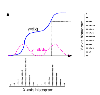
Figure 1: Illustration of an activation function removing modality in data when the derivative approximates the histogram.

The view that $f(x)$ is a PDF estimator, and the fact that data often has clusters leads us to the idea of creating AF’s with multi-modal derivatives. One of the simplest and earliest types of AFs is the sigmoid function, whose derivative approximates a Gaussian distribution. Therefore, the sum of shifted sigmoid functions approximates a Gaussian mixture, which is a popular approach to PDF estimation [7, 8]. Different base activation functions lead to other mixture distributions. This view leads us to the idea for the trained compound activation functions (TCA).

I-C Contributions and Goals of Paper

In this paper, we propose TCA, a trainable activation function with complex, but monotonic response. We argue that using a TCA in a neural network, is a more efficient way to increase the effectiveness of a network than adding layers. Furthermore, in generative networks, the TCA has an interpretation as a mixture distribution and can remove modality in the data. When the TCA is used in a restricted Boltzmann machine (RBM), it creates a novel type of RBM based on stochastic units that are mixtures. We show significant improvement of TCA-based RBMs, deep belief network (DBN) and projected belief networks (PBNs) in experiments.

II Trained Compound Activation Function (TCA)

Consider the compound activation function $f(x)$ given by

$$f(x)=\frac{1}{M}\sum_{j=1}^{M}\;f_{0}\left(e^{a_{j}}x+b_{j}\right),$$ (5)

where $f_{0}(x)$ is the base activation function, and ${\bf a}=\{a_{j}\}$ and ${\bf b}=\{b_{j}\}$ are scale and bias parameters. The exponential function $e^{a_{j}}$ is used to insure positivity of the scale factor. Note that if $f_{0}(x)$ is a monotonically increasing function (which we always assume), then the TCA is monotonically increasing and equal to the base activation function if ${\bf a}={\bf 0}$ and ${\bf b}={\bf 0}$.

For a dimension-$N$ input data vector ${\bf x}$, the TCA operates element-wise on ${\bf x}$ as follows:

$${\bf y}=f({\bf x}),\;\;\;y_{i}=\frac{1}{M}\sum_{j=1}^{M}\;f_{0}\left(e^{a(i,j)}x_{i}+b(i,j)\right),\;1\leq i\leq N,$$ (6)

where ${\bf A}=\{a(i,j)\}$ and ${\bf B}=\{b(i,j)\}$ are $N\times M$ scale and bias parameters. A TCA can be implemented with an additional dense layer that expands the dimension to $N\cdot M$ neurons, followed by a linear layer that averages over each group of $M$ neurons, compressing back to dimension $N$. But, not only does a TCA use a factor of $N$ fewer parameters, but it has an interpretation as a mixture distribution when used in generative models, and results in a novel type of RBM, as we now show.

III TCA for Deep Belief Networks (DBN)

A deep belief network is a layered network proposed by Hinton [9] based on restricted Boltzmann machines (RBMs).

III-A RBMs

The RBM is a widely-used generative stochastic artificial neural network that can learn a probability distribution over its set of inputs [10]. The RBM is based on an elegant stochastic model, the Gibbs distribution, and is the central idea in a deep belief network (DBN) made popular by Hinton [9]. A cascaded series of layer-wise-trained RBMs can be used to initialize deep neural networks. This method, in fact played a key role in the birth of deep learning because they provided a means to pre-train deep networks that suffered from vanishing gradients.

III-B Review of RBMs

The RBM estimates a joint distribution between an input (visible) data vector ${\bf x}\in\mathbb{R}^{N}$, and a set of hidden variables ${\bf h}\in\mathbb{R}^{M}$. The RBM consists of a pair of stochastic perceptrons, arranged back-to-back, and is illustrated in Figure 2.

Figure 2: Illustration of an RBM.

In a sampling procedure called “Gibbs sampling”, data is created by alternately sampling ${\bf x}$ and ${\bf h}$ using the conditional distributions $p_{h}({\bf h}|{\bf x})$ and $p_{x}({\bf x}|{\bf h})$. To sample ${\bf h}$ from the distribution $p_{h}({\bf h}|{\bf x})$, we first multiply ${\bf x}$ by the transpose of the $N\times M$ weight matrix ${\bf W}$, and add a bias vector: $\mbox{\boldmath$\alpha$}={\bf W}^{\prime}{\bf x}+{\bf b}.$ The variable $\alpha$ is then applied to a generating distribution (GD) to create the stochastic variable ${\bf h}$ as $h_{i}\sim p(h;\alpha_{i}),$ $1\leq i\leq M$. Note that conditioned on ${\bf x}$, ${\bf h}$ is a set of independent random variables (RV). To sample ${\bf x}$ from the distribution $p_{x}({\bf x}|{\bf h})$, we use the analog of the forward sampling process: $\mbox{\boldmath$\beta$}={\bf W}{\bf h}+{\bf a}.$ The variable $\beta$ is then applied to a generating distribution $x_{j}\sim p(x;\beta_{j}),$ $1\leq j\leq N$. Conditioned on ${\bf h}$, ${\bf x}$ is a set of independent random variables (RV). After many alternating sampling operations, the joint distribution between ${\bf x}$ and ${\bf h}$ converges to the Gibbs distribution $p({\bf x},{\bf h})=\frac{e^{-E({\bf x},{\bf h})}}{K},$ where the normalizing factor $K$ is generally unknown. Training an RBM is done using contrastive divergence, which is described in detail for exponential-class GDs in [11].

III-C Activation functions and RBMs

Once an RBM is trained, it can be used as a layer of a neural network to extract information-bearing features ${\bf h}$. This is done by replacing stochastic sampling with deterministic sampling by replacing the stochastic generating distributions $p(x;\beta)$, $p(h;\alpha)$ with activation functions that equal the expected value (mean) of the generating distributions, $f(x;\alpha)=\mathbb{E}(x;\alpha)$. Consider the Bernoulli distribution whose AF is the sigmoid function, the truncated exponential distribution (TED) whose AF is the TED distribution [12], the truncated Gaussian distribution (TG) whose AF is the TG activation [13], and the Gaussan distribution which has the linear AF $f(x)=x$.

III-D RBMs based on TCA

If a simple activation function corresponds to the expected value of the GD, then what distribution corresponds to a TCA? It is previously known that any monotonically-increasing function can be seen as a sum of shifted stochastic generating distributions [14, 2]. But, we must look more carefully at this because it is not as simple as adding random variables. When adding random variables, the probability densities combine by convolution, not additively. To combine them properly, we need a mixture distribution. Let $p_{0}(x;\alpha)$ be a univariate generating distribution depending on parameter $\alpha$, and let this distribution have mean $f_{0}(\alpha)=\mathbb{E}(x;\alpha)$, so $f_{0}(\alpha)$ is the AF corresponding to probability distribution $p(x;\alpha)$. Let $\Phi_{0}(x;\alpha)$ be the cumulative distribution function (CDF) of $p_{0}(x;\alpha)$ , i.e.

$$\Phi_{0}(x;\alpha)=\int_{-\infty}^{x}\;p_{0}(x;\alpha)\;{\rm d}x.$$

Now, consider a mixture distribution given by

$$p(x;\alpha)=\sum_{j=1}^{M}\;\frac{1}{M}\;p_{0}\left(e^{a_{j}}\alpha+b_{j}\right).$$ (7)

To draw a sample from mixture distribution (7), we first draw a discrete random variable $j$ uniformly in $[1,\;M]$, then draw $x$ from distribution $e^{-a_{j}}p_{0}\left(e^{a_{j}}\alpha+b_{j}\right)$. Mixture distribution (7) has CDF

$$\Phi(x;\alpha)=\frac{1}{M}\sum_{j=1}^{M}\;e^{-a_{j}}\Phi_{0}\left(e^{a_{j}}\alpha+b_{j}\right).$$ (8)

It is easily seen by taking the derivative, that distribution corresponding to the CDF (8) is (7). And, since expected value is a linear operation, the mean of distribution (7) is the TCA (5). Note that RBMs are implicitly an infinite mixture distributions over the hidden variables [15], but using using discrete mixture $\phi(x;\alpha)$ for a generating distribution creates an entirely novel type of RBM.

Different base AFs (i.e. different base stochastic units) can be used for the input and output, producing a wide range of different types of RBMs [13]. Figure 3 illustrates an RBM constructed using a TCA unit in the forward path. The activation functions and TCAs in the figure can be either stochastic (random sampling from the corresponding GD) or deterministic if the activation functions are used. In the forward path, a weight matrix ${\bf W}$ multiplies the input data vector ${\bf x}$ in order to produce a linear feature vector, which is then passed through the TCA to produce the hidden variables vector ${\bf h}$. In the backward path, ${\bf h}$ is multiplied by the transposed weight matrix ${\bf W}^{\prime}$ and passed through an activation function to produce the re-sampled input vector ${\bf x}$. In our approach, we use a TCA only in the forward path, with a normal AF in the backward path.

The mathematical approach to train the parameters of RBMs using the contrastive divergence (CD) algorithm is well documented [11] and can be extended in order to obtain the updates equations to train the parameters of the TCAs. This is facilitated using the symbolic differentiation available using software frameworks such as THEANO [16].

Figure 3: Illustration of an RBM based with TCA units in the forward path. The need for a separate bias in the forward path is eliminated due to the existance of trainable bias (shifts).

IV Stacked RBM and DBNs

To create a “stacked RBM”, an RBM is trained on the input data, and then the forward path is used to create hidden variables, which are then used as input data for the next layer. The deep belief network (DBN) [9] consists of a series of stacked RBMs, plus a special “top layer” RBM. The one-hot encoded class labels are injected at the input of the top layer (concatenated with the hidden variables from the last stacked RBM). Then, the Gibbs distribution of the top layer learns the joint distribution of the class labels with the hidden variables out of the last stacked RBM. The cleverness of Hinton’s invention lies in the fact that although the scale factor of the the Gibbs distribution is not known, it is not needed to compare the likelihood function from the competing class hypotheses. Computing the Gibbs distribution for a given class assumption has been called the “free energy” [9, 13], so we will call this a free energy classifier. Computing the free energy classifier requires solving for terms of the marginalized Gibbs distribution [13], and these in turn require the CDF, which we have given in (8). We therefore have all the tools to create a DBN using TCA-based stochastic units.

V Experiments: TCA-based RBM and DBN

V-A Data

For the these experiments, we took a subset of the MNIST handwritten data corpus, just three characters “3”, “8”, and “9”. The data consists of sample images of $28\times 28$, or a data dimension of 784. We used 500 training samples from each character. Since MNIST pixel data is coarsely quantized in the range [0,1], a dither was applied to the pixel values.

V-B Network

The network was a 1-layer stacked RBM of 32 neurons, followed by a top-level (classifier) RBM of 256 units. TCA’s with 3 components were used in the forward path. For the base activation and stochastic unit, truncated exponential distribution (TED), which is the continuous version of the Bernoulli distribution/sigmoid function [12, 13], is used.

V-C First Layer

In the first experiment, we trained just the first layer RBM and measured input data reconstruction error after one Gibbs sampling cycle. We consider both mean-square error and conditional likelihood function (LF) which is $\log p({\bf x}|\mbox{\boldmath$\beta$})$, where $\beta$ is the input to the activation functions in the reconstruction path (see Figure 3).

We trained in three phases, (a) first with no TCA (using just the base AF), then (b) with TCA but with TCA update disabled, then finally (c) with TCA enabled. At initialization, the TCAs have a transfer function very similar to the base non-linearity, so with TCA update disabled, we should expect the same performance as for the base AF. Training was done using contrastive divergence [11, 9]. For the first layer, we used deterministic Gibbs sampling (using AF instead of stochastic units). When switching from phase (b) to (c), we plotted the MSE as a function of epochs. In Figure 5, the plot begins where phase (b) has reached convergence, then at X axis -2.25, the TCA training is enabled and a drastic change is seen. In Table 5, we listed the final MSE and LF for the three phases. Nearly a factor of 2 reduction in MSE is seen. The improved reconstruction of TCA can be seen on the bottom row.

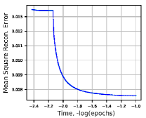
Figure 4: First layer mean square reconstruction error (MSE) as a function of training epoch with log-time in X-axis. After convergence at X-axis location -2.15, the TCAs were allowed to change.

AF	MSE	LF
TED	.0135	-7.0
TCA-0	.0134	-7.0
TCA	.0029	-2.59

Figure 5: MSE and conditional LF for first layer only. TCA-0: initial (but not updated) TCA.

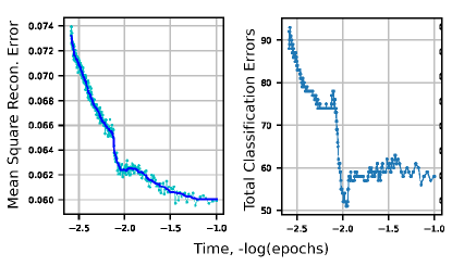
Figure 6: Training profile for the up-down algorithm where it can be seen that when enabling TCA, both reconstruction error and validation classfier errors decrease suddenly. The X-axis is minus the log of the number epochs in the past. Errors are on 1500 validation samples.

V-D DBN performance

The output of the first layer (using TCA) was applied to the second layer, with one-hot encoded labels injected, forming a DBN. We then trained the second layer using contrastive divergence (CD) with three Gibbs iterations and an added term of direct free energy (FE) cost function as proposed in [13]. Finally, the entire network was fine-tuned using the up-down algorithm, which is an extension of CD to the entire deep belief network [9]. The TCA was initialized so that it has a characteristic similar to the base activation. Then at some point, we enabled TCA training. In Figure 6, it can be see at X-axis -2.1, that TCA training was enabled, resulting in a sudden improvement of both reconstruction error number of and classifier errors measured on separate validation data.

VI TCA for Projected Belief Network and Auto-Encoders

VI-A Description

The projected belief network (PBN) is a generative network that is based on PDF estimation, a direct extension of (2), (4) to dimension-reducing transformations [6], so it is the ideal paradigm to test the concepts of TCA. The PBN is based on the idea of back-projection through a given feed-forward neural network (FFNN), a way to reconstruct or re-sample the input data based on the network output [17]. There are both stochastic and deterministic versions of the PBN [18]. In the stochastic PBN, a tractable likelihood function (LF) is computed for the FFNN, and inserting a TCA into the FFNN applies a term to the LF corresponding to the derivative of the TCA, which is a mixture distribution. The deterministic PBN (D-PBN) operates similarly, but is trained not to maximize the LF, but to maximize the conditional LF (given the network output), which is a probabilistic measure of the ability to reconstruct the input data. The D-PBN can be seen as an auto-encoder (AEC), so we will compare it with standard auto-encoders. We used the same data as in Section V-A.

VI-B Network

The network which is illustrated in Figure 7 had two dense perceptron layers with 32 and 8 neurons, respectively, and TCAs. The base non-linearity for the TCA was TED.

Figure 7: Illustration of a two-layer feed-forward network based on TCAs.

VI-C Results

We trained the network as an AEC, a VAE, and as a D-PBN using PBN Toolkit [19]. Note that in the VAE, a TCA is not used in the the output layer, because the output layer in a VAE has a special form. The output TCA is also not used in the D-PBN, since back projection starts with the output of the last linear transformation. In all cases, we trained to convergence with TCA training disabled, that is with the equivalent of a simple AF, then again with TCA training enabled. We report mean square error (MSE) on training and test data in Table I.

Algorithm	TCA	MSE(train)	MSE(test)
AEC	No	.02024	.02273
AEC	Yes	.01884	.02403
VAE	No	.02220	.02509
VAE	Yes	.01835	.02179
D-PBN	No	.01917	.01955
D-PBN	Yes	.01790	.01790

Table I: Mean square reconstruction error for various auto-encoders.

We may make a number of conclusions from the table. First, using TCA significantly improves performance in all cases (compare “Yes” rows to ‘No” rows). Second, the D-PBN has not only best performance, but it generalizes much better than conventional auto-encoders, a feature of D-PBN that we have reported prevously [18]. In this case, there was almost no measureable difference between training and test data. As we explained, both the VAE and D-PBN do not use the final TCA, so the performance difference hinges only on the TCA at the output of the first layer. Despite this, a significant improvement is seen.

VI-D TCA vs Added Network Layers

The performance improvements of TCA in a standard feed-forward or plain auto-encoder can be attributed to the increased parameter count over standard activation functions, but a TCA achieves this with far fewer parameters than adding layers. Furthermore, in RBMs and DBNs, using TCAs creates novel generative models with stochastic units based on finite mixture distributions, something that cannot be achieved by adding network layers. Using TCAs, it is seen that RBMs and DBNs have significantly better performance.

VII Conclusions

In this paper, we have introduced trained compound activations (TCAs). We justified their use based on PDF estimation and removal of modalities. We have derived novel restricted Boltzmann machines (RBMs) based on TCAs, and have demonstrated convincing improvements for TCAs in experiments using stacked RBMs, deep belief networks (DBNs), auto-encoderes and deterministic projected belief networks (D-PBNs). All experiments were implemented using PBN Toolkit [19]. All data, software, and instructions to repeat the results in this paper are archived at [19].

References

- [1] J. Feng and S. Lu, “Performance analysis of various activation functions in artificial neural networks,” in Journal of Physics Conference Series, no. 1237, 2019.
- [2] S. Ravanbakhsh, B. Póczos, J. Schneider, D. Schuurmans, and R. Greiner, “Stochastic neural networks with monotonic activation functions,” Proceedings of the 19 th International Conference on Artificial Intelligence and Statistics (AISTATS), Cadiz, Spain, 2016.
- [3] Y. Wang, Y. Li, Y. Song, and X. Rong, “The influence of the activation function in a convolution neural network model of facial expression recognition,” Applied Sciences, vol. 10, p. 1897, 03 2020.
- [4] X. Jin, C. Xu, J. Feng, Y. Wei, J. Xiong, and S. Yan, “Deep learning with s-shaped rectified linear activation units,” in Proceedings of the AAAI Conference on Artificial Intelligence, vol. 30, 2016.
- [5] K. He, X. Zhang, S. Ren, and J. Sun, “Delving deep into rectifiers: Surpassing human-level performance on imagenet classification,” 2015.
- [6] P. M. Baggenstoss and S. Kay, “Nonlinear dimension reduction by pdf estimation,” (Accepted in) IEEE Transactions on Signal Processing, 2022.
- [7] R. A. Redner and H. F. Walker, “Mixture densities maximum likelihood, and the EM algorithm,” SIAM Review, vol. 26, April 1984.
- [8] G. J. McLachlan, Mixture Models. Dekker, 1988.
- [9] G. E. Hinton, S. Osindero, and Y.-W. Teh, “A fast learning algorithm for deep belief nets,” in Neural Computation 2006, 2006.
- [10] I. Goodfellow, Y. Bengio, A. Courville, and Y. Bengio, Deep Learning. Cambridge, MA: MIT press, 2016.
- [11] M. Welling, M. Rosen-Zvi, and G. Hinton, “Exponential family harmoniums with an application to information retrieval,” Advances in neural information processing systems, 2004.
- [12] P. M. Baggenstoss, “Evaluating the RBM without integration using pdf projection,” in Proceedings of EUSIPCO 2017, Island of Kos, Greece, Aug 2017.
- [13] P. Baggenstoss, “New restricted Boltzmann machines and deep belief networks for audio classification,” 2021 ITG Speech Communication, Kiel (Virtual), 2021.
- [14] V. Nair and G. E. Hinton, “Rectified linear units improve restricted boltzmann machines,” Proceedings of the 27th International Conference on Machine Learning, Haifa, Israel, 2010, 2010.
- [15] N. Roux and Y. Bengio, “1 representational power of restricted boltzmann machines and deep belief networks,” Neural computation, vol. 20, pp. 1631–49, 07 2008.
- [16] J. Bergstra, O. Breuleux, F. Bastien, P. Lamblin, R. Pascanu, J. Turian, D. Warde-Farley, and Y. Bengio, “Theano: A cpu and gpu math expression compiler,” Proceedings of the Python for Scientific Computing Conference (SciPy), 2010.
- [17] P. M. Baggenstoss, “On the duality between belief networks and feed-forward neural networks,” IEEE Transactions on Neural Networks and Learning Systems, pp. 1–11, 2018.
- [18] P. M. Baggenstoss, “Applications of projected belief networks (PBN),” Proceedings of EUSIPCO, A Corunã, Spain, 2019.
- [19] P. Baggenstoss, “PBN Toolkit,” {http://class-specific.com/pbntk}. Accessed: 2022-02-28.