Robust Audio-Visual Instance Discrimination via Active Contrastive Set Mining

Abstract

The recent success of audio-visual representation learning can be largely attributed to their pervasive property of audio-visual synchronization, which can be used as self-annotated supervision. As a state-of-the-art solution, Audio-Visual Instance Discrimination (AVID) extends instance discrimination to the audio-visual realm. Existing AVID methods construct the contrastive set by random sampling based on the assumption that the audio and visual clips from all other videos are not semantically related. We argue that this assumption is rough, since the resulting contrastive sets have a large number of faulty negatives. In this paper, we overcome this limitation by proposing a novel Active Contrastive Set Mining (ACSM) that aims to mine the contrastive sets with informative and diverse negatives for robust AVID. Moreover, we also integrate a semantically-aware hard-sample mining strategy into our ACSM. The proposed ACSM is implemented into two most recent state-of-the-art AVID methods and significantly improves their performance. Extensive experiments conducted on both action and sound recognition on multiple datasets show the remarkably improved performance of our method.

1 Introduction

Visual scenes are typically synchronised with a mixture of sounds, for instance moving lips and speech or moving cars and engine noiseXuan et al. (2020). This pervasive audio-visual synchronization comes from the fact that sound is produced by the vibration of objects. Through such an audio-visual synchronised perception Smith and Gasser (2005), humans are capable of developing skills to better perceive the world. As for machine intelligence, audio-visual synchronization in videos also raises the possibility to develop similar skills by investigating audio-visual representation learning. In addition, different from expensive and subjective manual annotations, audio-visual synchronization provides free and extensive self-annotated supervisions for exploring audio-visual representation learning using numerous videos available on the Internet.

Recent studies on self-supervised audio-visual representation learning Arandjelovic and Zisserman (2017, 2018); Korbar et al. (2018); Owens and Efros (2018) set up a binary verification problem that predicts whether an input audio-visual pair is correct, that is an “in-sync” video and audio, or incorrect, that is constructed by using “out-of-sync” audio Korbar et al. (2018) or audio from a different video Arandjelovic and Zisserman (2017). However, exploiting one single pair at a time loses the key opportunity to reason about the data distribution in large-scale.

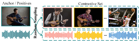
Figure 1: Illustration of a contrastive set constructed by randomly sampling in AVID. Such a random sampling relies on one key assumption: the audio and visual clips from all other videos are not semantically related. The contrastive set with such faulty negatives undermines the primary goal of AVID, i.e. we cannot keep the visual clips with guitar playing and the audio with guitar strumming both far away from and close to each other in the representation space.

To alleviate the above issue, some works have attempted to improve upon the binary verification problem by posing it as an Instance Discrimination (ID) Jaiswal et al. (2021) task, called Audio-Visual Instance Discrimination (AVID). Specifically, Morgado et al. (2021a, b) propose a cross-modal version of ID and Ma et al. (2021) present a multi-modal extension of Momentum Contrast (MoCo) He et al. (2020). They have achieved impressive performance on AVID through constructing a contrastive set with large negatives by randomly sampling from a memory bank Wu et al. (2018) or a queue-based dictionary He et al. (2020). The reasons for the success are two-fold: on one hand, the introduction of a contrastive set rather than a single pair facilitates reasoning about the data distribution. On the other hand, memory bank and dictionary decouple the size of the contrastive set from the mini-batch size, allowing it to be large. Theoretically, a large contrastive set can achieve a tighter lower bound on Mutual Information (MI) McAllester and Stratos (2020).

However, these methods rely on one key assumption when constructing the contrastive set for AVID: the audio and visual clips from all other videos are not semantically related. In practice, such an assumption does not hold for a significant amount of real-world videos. Simply increasing the size of the contrastive set beyond a threshold does not improve or even harm the performance of learned representations on downstream tasks Saunshi et al. (2019). We argue that such a contrastive set, constructed by randomly sampling rather than carefully designing, is much responsible for this: as shown in Fig.1, it can lead to faulty negatives (semantically related to the anchor). The contrastive set with such faulty negatives undermines the primary goal of AVID, i.e., we cannot keep the audio-visual pairs with related semantics both far from and close to each other in the representation space. Also, this issue can get aggravated as the size of the contrastive set increases.

For this purpose, we propose a method called Active Contrastive Set Mining (ACSM) that aims to mine the contrastive sets with informative and diverse negatives for robust AVID. Specifically, the semantic structures are explicitly imposed to unlabelled audio-visual clips to encourage learning a “semantics-aware” discriminative space. At this point, the contrastive set can be constructed under the guidance of progressive semantics during the training of our ACSM. Different from the existing AVID Morgado et al. (2021a, b); Ma et al. (2021) which pull away each audio or visual clips from all other videos in the representation space, our ACSM takes also the diverse semantics into account, i.e., only the audio-visual pairs with diverse semantics are far away from each other. Moreover, benefiting from our semantics-aware beyond instance-specific AVID, we introduce semantic ambiguity, rather than simple time gaps Bruno et al. (2018), to mine hard samples, which can be easily integrated into AVID. In summary, the main contributions of this work are re-emphasised as follows:

• An active contrastive set mining (ACSM) is proposed for mining the contrastive sets with informative and diverse negatives for robust AVID;

• We elegantly extend our ACSM to two state-of-the-art AVID methods, i.e., Cross-modal ID Ma et al. (2021) and Multi-modal MoCo Morgado et al. (2021a, b), which then achieves significant improvements;

• With the semantics from our ACSM, a hard sample mining strategy based on the semantic ambiguity is introduced to boost discriminative ability of AVID.

Extensive experiments and remarkable performance gains show the effectiveness of our method. Our method also achieves state-of-the-art transfer learning performance, both action recognition on UCF101 and HMDB51 datasets and sound recognition on ESC-50 and DCASE datasets, when pre-training on the subset of Audioset dataset.

2 Related Work

Instance Discrimination

conducts contrastive learning by treating each sample as a separate class and pulling the positives (“similar”) closer while pushing the negatives (“dissimilar”) far away to learn instance-specific discriminative representation. MoCo He et al. (2020) adopts an online encoder and a momentum encoder to receive two views of a sample as positive pairs. A queue-based dictionary is built to store negative samples. SimCLR Chen et al. (2020a) pushes self-supervised pre-training to comparable effects as the supervised methods. They also carefully sort out the tricks for effective training, such as longer training time or stronger data augmentation. Chen et al. (2020b) proposes MoCo-v2 and refreshes the performance of self-supervised learning once again. BYOL Grill et al. (2020) adds a predictor to learn the map from the online encoder to the momentum encoder instead of displaying positive samples. Through the stop gradient mechanism, they skillfully discard the negatives. Simsiam Chen and He (2021) lets the target encoder and the online encoder be the same and points out that the predictor and the stop gradient mechanism are sufficient conditions for self-supervised training.

These works rely heavily on proper data augmentation setups. Instead, we focus on cross-modal instance discrimination, which avoids this issue through the inherent and pervasive synchronization between audio-visual messages. Furthermore, our goal is to be “semantics-aware”, not just instance-specific instance discrimination by introducing the idea of deep clustering Zhan et al. (2020).

Self-Supervised Audio-Visual Representation Learning.

Besides computer vision, several approaches attempt to learn audio-visual representations in a self-supervised manner. Arandjelovic and Zisserman (2017, 2018) propose to learn audio-visual representations by solving a binary verification problem that predicts whether the input audio-visual pair is matched or not. Korbar et al. (2018); Owens and Efros (2018) predict if audio-visual clips are synchronized in time, and Morgado et al. (2020) predicts if the audio-visual clips extracted from the $360^{\circ}$ videos are aligned in space. Morgado et al. (2021a, b); Ma et al. (2021) improve upon the binary verification problem by posing it as an instance discrimination task, where the size of the contrastive set is decoupled from the mini-batch size, allowing it to be large. In this paper, we explore an online mining strategy, rather than random sampling, to construct a reliable contrastive set.

3 Audio-Visual Instance Discrimination

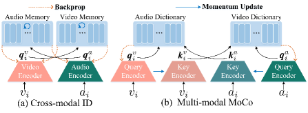
Figure 2: The diagram of Cross-modal ID Morgado et al. (2021a, b) and Multi-modal MoCo Ma et al. (2021), where $(a_{i},v_{i})$ denotes the input audio-visual pair. We use $f(\cdot)$ indicates the query encoder with learnable parameters $\bm{\theta}$, updated by the gradients, and $h(\cdot)$ represents the key encoder with learnable parameters $\bm{\delta}$, updated by the momentum. The superscript is used to distinguish various data streams from audio or visual modality, where the query encoder and key encoder from the same modality have the same structure but independent parameters. Formally, the formulation can be expressed as: $\textbf{\emph{q}}_{i}^{v}=f^{v}(v_{i};\bm{\theta}^{v})$, $\textbf{\emph{q}}_{i}^{a}=f^{a}(a_{i};\bm{\theta}^{a})$, $\textbf{\emph{k}}_{i}^{v}=h^{v}(v_{i};\bm{\delta}^{v})$ and $\textbf{\emph{k}}_{i}^{a}=h^{a}(a_{i};\bm{\delta}^{a})$.

Let $(A,V)$ be a collection of $N$ videos, where $A=\{a_{i}\}_{i=1}^{N}$, $V=\{v_{i}\}_{i=1}^{N}$, each audio-visual pair $\{a_{i},v_{i}\}$ is from the same block of a video. Here, $a_{i}\in\mathbb{R}^{H_{a}\times W_{a}}$ refers to the spectrogram of the raw audio waveform, where $H_{a}$ is time step and $W_{a}$ is frequency band. $v_{i}\in\mathbb{R}^{F\times 3\times H_{v}\times W_{v}}$ is the visual clip containing $F$ RGB frames with a height of $H_{v}$ and a width of $W_{v}$. The learning objective of AVID is to encourage the representations of audio-visual clips to be similar if they come from the same temporal block of a video and vice-versa.

Formally, AVID employs a Noise-Contrastive Estimation (NCE) Gutmann and Hyvärinen (2010) to learn two encoders independently, $f(\cdot;\bm{\theta})$ and $h(\cdot;\bm{\delta})$, by matching $\textbf{\emph{q}}_{i}$ with $\textbf{\emph{k}}_{i}$ against its contrastive set $\mathcal{K}_{i}=\{\textbf{\emph{k}}_{j}^{i}\}_{j=1}^{K}$:

$$\mathcal{L}_{nce}(\textbf{\emph{q}}_{i};\textbf{\emph{k}}_{i},\mathcal{K}_{i})=-\log\frac{\exp[\cos(\textbf{\emph{q}}_{i},\textbf{\emph{k}}_{i})/\tau]}{\sum_{\tilde{\textbf{\emph{k}}}}\exp[\cos(\textbf{\emph{q}}_{i},\tilde{\textbf{\emph{k}}})/\tau]},$$ (1)

where $\textbf{\emph{q}}_{i}=f(\cdot)$ and $\textbf{\emph{k}}_{i}=h(\cdot)$ are the outputs of query encoder $f$ and key encoder $h$ with parameters $\bm{\theta}$ and $\bm{\delta}$ respectively, $\tilde{\textbf{\emph{k}}}\in\mathcal{K}_{i}\cup\{\textbf{\emph{k}}_{i}\}$, $\cos(\cdot,\cdot)$ is the cosine similarity between a pair of representations, $\tau$ is the temperature to control the concentration degree of distribution and $K$ is the size of the contrastive set.

Minimising NCE loss means maximising a lower bound on the MI between audio-visual pairs, which allows the model to learn to discriminate whether audio-visual pairs are “similar” or “dissimilar”. The final objective $\mathcal{L}_{nce}$ of AVID consists of two terms:

$$\mathcal{L}_{nce}=\mathcal{L}_{nce}(\textbf{\emph{q}}_{i}^{v};\textbf{\emph{k}}_{i}^{a},\mathcal{K}_{i}^{a})+\mathcal{L}_{nce}(\textbf{\emph{q}}_{i}^{a};\textbf{\emph{k}}_{i}^{v},\mathcal{K}_{i}^{v}),$$ (2)

where the former indicates visual-to-audio component and the latter refers to audio-to-visual component.

There are two most recently proposed approaches for performing AVID, i.e., Cross-modal ID Morgado et al. (2021a, b) and Multi-modal MoCo Ma et al. (2021). The diagram of these two approaches is depicted in Fig.2. We make a brief summary of the main differences and connections between the two.

Momentum Update.

As shown in Fig.2, both Cross-modal ID and Multi-modal MoCo employ a momentum update to maintain consistency during training:

$$\textbf{\emph{u}}_{{}_{old}}\leftarrow m\textbf{\emph{u}}_{{}_{old}}+(1-m)\textbf{\emph{u}}_{{}_{new}},$$ (3)

where $m\in[0,1)$ is a momentum coefficient, u is the content to be updated. The former utilizes a momentum-based moving average memory bank Wu et al. (2018), while the latter exploits a momentum-based slowly-changing encoder. Besides, Multi-modal MoCo performs a cross-modal online dictionary look-up, i.e., the encoded representations of the current mini-batch are enqueued and the oldest ones are dequeued.

Given a query, its contrastive set $\mathcal{K}_{i}$ in Eq.1 is constructed by randomly sampling from a semantically indistinguishable memory bank or queue-based dictionary as there are no annotations available. Such a random sampling strategy makes the contrastive set contain massive faulty negatives and undermines the primary goal of AVID, resulting in no improvement or even impairment when simply increasing the size of the contrastive set.

4 Active Contrastive Set Mining

We believe that the random sampling without semantic guidance is the main cause of the above problem when constructing the contrastive set. For this purpose, we introduce a novel semantic-sensitive library for mining the contrastive set with informative and diverse negatives for robust AVID. Such libraries serve three functions:

• playing the role of conventional memory bank or dictionary to store a series of representations on-the-fly;

• imposing the underlying semantic structures on the audio and visual samples;

• providing the semantic guidance when constructing the contrastive set.

To be concrete, different from a single library with semantic mixtures, we manage $C$ independent libraries $\mathcal{M}=\{M_{m}\}_{m=1}^{C}$, where each library $M_{m}$ corresponding to one semantics. They are constructed by a learnable classifier that predicts the pseudo-label of a query. For a query $\textbf{\emph{q}}_{i}$ with pseudo-label $y_{i}$, we can construct its contrastive set $\mathcal{K}_{i}$ in a manner similar to supervised contrastive learning Khosla et al. (2020):

$$\mathcal{K}_{i}=\{\hat{\textbf{\emph{k}}_{j}}~{}|~{}\hat{\textbf{\emph{k}}_{j}}\in M_{m},~{}\forall~{}m\neq y_{i}\},$$ (4)

where $j\in[1,K]$ and $m,y_{i}\in[1,C]$. After every backward pass, its key $\textbf{\emph{k}}_{i}$ is used to update the corresponding $M_{y_{i}}$ in a queue-based or momentum-based manner.

Table 1: Top-1 accuracy of action recognition on UCF-101 and HMDB-51 datasets.

Methods	Pretraining Dataset	Finetune Resolution	Architecture	UCF-101	HMDB-51
Shuffle&Learn Misra et al. (2016)	UCF-101	$1\times 227^{2}$	CaffeNet	$50.2$	$18.1$
OPN Lee et al. (2017)				$56.3$	$23.8$
ST-Order Buchler et al. (2018)			VGG	$58.6$	$25.0$
CMC Tian et al. (2020)			3D-ResNet18	$59.1$	$26.7$
CBT Sun et al. (2019)	Kinetics-600	$16\times 122^{2}$	S3D & BERT	$79.5$	$44.6$
3D-RotNet Jing et al. (2018)	Kinetics-400		3D-ResNet18	$62.9$	$33.7$
ClipOrder Xu et al. (2019)			R(2+1)D-18	$72.4$	$30.9$
DPC Han et al. (2019)		$25\times 128^{2}$	3D-ResNet34	$75.7$	$35.7$
$L^{3}$-Net Arandjelovic and Zisserman (2017)		$16\times 224^{2}$	2D-Conv	$74.4$	$47.8$
AVTS Korbar et al. (2018)		$25\times 224^{2}$	MC3	$85.8$	$56.9$
XDC Alwassel et al. (2018)		$8\times 224^{2}$	R(2+1)D-18	$74.2$	$39.0$
xID Morgado et al. (2021b)				$82.3$	$49.1$
Robust-xID Morgado et al. (2021a)				$81.9$	$49.5$
xID + CMA Morgado et al. (2021b)				$83.7$	$50.2$
MmMoCo Ma et al. (2021)				$83.5$	$49.4$
MmMoCo + AS Ma et al. (2021)				$85.6$	$58.6$
xID + ACSM (Ours)				$\bm{86.7}$	$\bm{60.4}$
MmMoCo + ACSM (Ours)				$\bm{88.4}$	$\bm{61.3}$

The samples with various pseudo-labels are put in separate libraries. As a result, one library can be viewed as one semantic “cluster”, where the samples in same library can be taken as anchors to describe this semantics. These semantic libraries can naturally serve as the semantic decision boundaries based on sample-anchor similarity:

$$g_{ij}=\frac{\sum_{\textbf{\emph{m}}\in M_{j}}\exp[\cos(\textbf{\emph{q}}_{i},\textbf{\emph{m}})/\tau]}{\sum_{m=1}^{C}\sum_{\textbf{\emph{m}}\in M_{m}}\exp[\cos(\textbf{\emph{q}}_{i},\textbf{\emph{m}})/\tau]},$$ (5)

Given a query $\textbf{\emph{q}}_{i}$ its similarity-based semantics assignments are represented as $\textbf{\emph{g}}_{i}=[g_{i1},\cdots,g_{ij},\cdots,g_{iC}]$, where $\textbf{\emph{g}}_{i}\in\mathbb{R}^{C}$. With such potential memberships, we can train the classifier which aims to minimise $\textbf{\emph{g}}_{i}$ and the semantics predictions $\textbf{\emph{p}}_{i}$, where $\textbf{\emph{p}}_{i}$ is yielded by the classifier $r(\cdot;\bm{\gamma})$ with the learnable parameters $\bm{\gamma}$, i.e., $\textbf{\emph{p}}_{i}=r(\textbf{\emph{q}}_{i})$. We propagate the gradient back to the classifier only to avoid feature learning from unreliable semantics. With the updated classifier $r(\cdot)$, we update the predicted semantics $y_{i}$ in a maximum likelihood manner for the contrastive set construction in Eq. 4. At the same time, the samples are assigned to the library with the most similar anchors and each library holds its own attribute that makes it different from the others.

Discussion.

Intuitively, at the beginning of training, the weak classifier provides near-random semantics predictions, so that our semantic libraries contain no semantic structures. At this point, the contrastive set constructed by Eq.4 approximates to a random sampling. With the progressive classifier, our semantic libraries cover increasingly clear semantic structures and provide effective semantic guidance when constructing the contrastive set, allowing our contrastive set to contain more informative and diverse negatives.

Furthermore, both Cross-modal ID Morgado et al. (2021a, b) and Multi-modal MoCo Ma et al. (2021) only optimise instance-specific discriminative representations, leading them to be not semantics sensitive and unaware of any potential non-linear intra-semantics variation. Compared with them, our ACSM maximises not only the instance-level diversity within the library, but also semantic-level compactness among libraries. The samples belonging to the same semantic library may share a common contrastive set. It means that the samples within the library are indirectly pushed closer in the representation space, resulting in more compact within-library representations.

Hard Sample Mining.

The samples that are easily discriminated by the current model tend to contribute less to instance discrimination Sheng et al. (2020). Hard sample mining is important in the instance discrimination field but is especially essential in the audio-visual field. From the information-theoretic perspective Chen et al. (2018), audio-visual messages in videos contain higher MI due to the higher dimensionality (i.e., temporal and multi-modal). The instances with higher MI mean that they are easier to discriminate. For this purpose, Bruno et al. (2018) perform the hard sample mining based on one key assumption: the smaller the time gap is between audio-visual clips of the same video, the harder it is to discriminate them. Instead of making such a assumption, we mine hard samples by emphasising the samples with ambiguous semantics. Given a query $\textbf{\emph{q}}_{i}$ with pseudo-label $y_{i}^{e}$ at $e$th epoch, its semantic ambiguity is denoted as:

$$s_{i}^{e}=s_{i}^{e-1}+1,\text{~{}if~{}}y_{i}^{e}\neq y_{i}^{e-1}$$ (6)

Those samples that are frequently swapped across semantics will be assigned higher weights in Eq.2 to provide more useful discriminative clues. Overall, we apply our ACSM to Cross-modal ID Ma et al. (2021) and Multi-modal MoCo Morgado et al. (2021a, b).

Table 2: Top-1 accuracy of sound recognition on ESC-50 and DCASE datasets.

Methods	Pretraining Dataset	Architecture	ESC-50	DCASE
Random Forest Piczak (2015b)	ESC-50	MLP	$44.3$	$-$
Piczak ConvNet Piczak (2015a)		ConvNet-4	$64.5$	$-$
ConvRBM Sailor et al. (2017)			$86.5$	$-$
Sound-Net Aytar et al. (2016)	SoundNet	ConvNet-8	$74.2$	$88$
$L^{3}$-Net Arandjelovic and Zisserman (2017)			$79.3$	$93$
AVTS Korbar et al. (2018)	Kinetics-400	VGG-8	$76.7$	$91$
XDC Alwassel et al. (2018)		ResNet-18	$78.5$	$-$
xID Morgado et al. (2021b)		ConvNet-9	$77.6$	$93$
xID + CMA Morgado et al. (2021b)			$79.1$	$93$
Robust-xID Morgado et al. (2021a)			$80.2$	$92.4$
MmMoCo Ma et al. (2021)			$78.8$	$93.6$
MmMoCo + AS Ma et al. (2021)			$86.4$	$94.3$
xID + ACSM (Ours)			$\bm{88.5}$	$\bm{95.2}$
MmMoCo + ACSM (Ours)			$\bm{89.3}$	$\bm{94.7}$

Table 3: Action recognition accuracy of linear probing on Kinetics and sound recognition accuracy of linear probing on ESC-50, where the evaluated representations come from various blocks of the encoder, $\color[rgb]{0,.5,.5}\uparrow$ indicates the increase in accuracy.

	Kinetics-400				ESC-50
Method	block1	block2	block3	block4	block1	block2	block3	block4
xID	$19.80$	$26.98$	$34.81$	$39.95$	$67.25$	$73.15$	$74.80$	$75.05$
xID + ACSM	$\color[rgb]{0,.5,.5}1.26\uparrow$	$\color[rgb]{0,.5,.5}1.69\uparrow$	$\color[rgb]{0,.5,.5}2.37\uparrow$	$\color[rgb]{0,.5,.5}3.56\uparrow$	$\color[rgb]{0,.5,.5}3.85\uparrow$	$\color[rgb]{0,.5,.5}5.56\uparrow$	$\color[rgb]{0,.5,.5}7.12\uparrow$	$\color[rgb]{0,.5,.5}8.71\uparrow$
MmMoCo	$20.12$	$26.48$	$35.35$	$39.75$	$66.86$	$72.69$	$74.93$	$76.56$
MmMoCo + ACSM	$\color[rgb]{0,.5,.5}0.94\uparrow$	$\color[rgb]{0,.5,.5}1.76\uparrow$	$\color[rgb]{0,.5,.5}2.68\uparrow$	$\color[rgb]{0,.5,.5}3.35\uparrow$	$\color[rgb]{0,.5,.5}4.11\uparrow$	$\color[rgb]{0,.5,.5}5.98\uparrow$	$\color[rgb]{0,.5,.5}6.94\uparrow$	$\color[rgb]{0,.5,.5}8.58\uparrow$

5 Experiments

For quantitative evaluation, we evaluate both the pre-trained visual and audio representations using transfer learning. Concretely, these pre-trained representations are evaluated by linear probing, i.e., keep the pre-trained network fixed and train linear classifiers.

5.1 Experimental Setups

Data preprocessing.

Video clips are extracted at a frame rate of $16$fps with some standard data augmentation strategies, i.e., random multi-scale cropping, random horizontal flipping, color jittering and temporal jittering.

For audio clips, each audio with a duration of $2$s is randomly sampled within $0.5$s at a $24$kHz sampling rate. Then, we convert the spectrogram of the audio track to a log scale, its intensity is $Z$-normalized using mean and standard deviation values obtained on the training set. Volume jittering and temporal jittering are used for audio augmentation.

Video and audio encoder.

We employ the R(2+1)D network Tran et al. (2018) with $18$ layers (Sect.5.2) or $9$ layers (Sect.5.3) as the video encoder and a 9-layer 2D CNN with batch normalization as the audio encoder. The outputs of the video encoder and audio encoder are max-pooled, projected into $128$ dimensions using an MLP, and then normalized into the unit sphere, where the MLP is composed of three FC layers with $512$ hidden units. We utilize the $128$-dimensional representation to update our semantic libraries.

Implementation details.

For fair comparisons, we follow the same settings of Morgado et al. (2021b). Respectively, the input of video encoder is set as $8$ frames of size $224\times 224$ (Sect.5.2) and $16$ frames of size $122\times 122$ (Sect.5.3). The spectrogram size is set as $200\times 257$ (Sect.5.2) and $100\times 129$ (Sect.5.3). We separately utilize Kinetics-$400$ dataset containing $240K$ videos (Sect.5.2) and Audioset dataset with a random sample of $100K$ videos (Sect.5.3) to pre-train our model. The temperature parameter $\tau$ in Eq.1 and Eq.5 is set to $0.07$. The momentum coefficient $m$ is set to $0.9$. The number of semantic libraries $C$ is set to $50$. The size of the contrastive set $K$ is set to $8192$. Each semantic-sensitive library stores $K/(C-1)$ representations. Our model is trained with the Adam optimizer for $400$ epochs with a learning rate of $1e-4$, weight decay of $1e-5$, and batch size of $256$. The parameters of the encoders, classifiers, and semantic libraries in our model are randomly initialised.

5.2 Comparisons with SOTAs

It is impractical to give a direct comparison to all approaches due to the enormous differences in the experimental setups, e.g., using diverse encoder architectures, pre-training on various datasets and fine-tuning with different resolutions. To empower solid comparisons, we list these differences for each method in Tab.1 and Tab.2, where Cross-modal ID and Multi-modal MoCo are abbreviated as xID and MmMoCo, respectively. The methods with the best and second-best performance are indicated in boldface.

Visual representations.

To evaluate the visual representations, we compare the transfer performance of action recognition with previous self-supervised methods on UCF-101 and HMDB-51 datasets. We follow Morgado et al. (2021b) and report top-1 accuracy of video-level predictions by averaging the clip-level accuracy of 10 uniformly sampled clips per test sample in Tab.1.

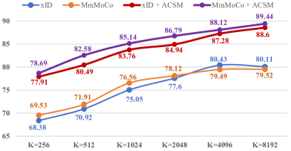
Figure 3: Effects of learning with different size of contrastive set $K$.

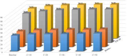
Figure 4: Effects of learning with different number of semantic libraries $C$. Both Cross-modal ID and Multi-modal MoCo are used as baselines.

Audio representations.

We evaluate the audio representations on ESC-50 and DCASE datasets for sound recognition. A linear one-vs-all SVM classifier is trained on the audio representations obtained by the pre-trained models at the final layer before pooling. We report top-1 accuracy of sample-level predictions by averaging 10 clip-level predictions in Tab.2.

As we can see, our approach outperforms other SOTA approaches. Compared with MmMoCo + ASMa et al. (2021), the current best performing method on self-supervised audio-visual representation learning, our model outperforms it by $2.8\%$ on UCF101, $2.7\%$ on HMDB51, $2.9\%$ on ESC-50 and $0.9\%$ on DCASE. Compared with xID Morgado et al. (2021b) and MmMoCo Ma et al. (2021) ($12$th and $15$th rows in Tab.2, $8$th and $11$th rows in Tab.1), our ACSM achieves impressive performance improvements on both action recognition and sound recognition.

5.3 Ablation Study

Random sampling vs. Active mining.

We evaluate the learned visual and audio representations in terms of the various blocks of the video and audio encoder. Separately, we employ the Kinetics-400 for action recognition and ESC-50 for sound recognition. Tab.3 reports the top-1 accuracy by averaging predictions over $25$ clips per video. Introducing our ACSM in Cross-modal ID and Multi-modal MoCo, the accuracy of both action recognition and sound recognition has been improved to varying degrees. The increase in recognition performance validates the benefits of a semantically sensitive library over a semantically indistinguishable one, resulting in better generalization of the learned representations to downstream tasks.

Hard Sample Mining.

We evaluate the learned visual and audio representations according to different hard sample mining strategies. We employ the representations from the block4 of the encoder to evaluate the performance of transfer learning on Kinetics-400 and ESC-50 datasets. Bruno et al. (2018) execute hard sample mining based on the time gap, i.e., $1\sim 200$ epochs with easy samples only and $201\sim 400$ epochs with $25\%$ hard samples and $75\%$ easy samples. To make fairer comparisons, we only execute our hard sample mining defined by Eq.6 in $201\sim 400$ epochs. The top-1 accuracy by averaging predictions over 25 clips per video is stated in Tab.4. As expected, hard sample mining improves the quality of learned representations. Compared with Bruno et al. (2018), our mining strategy based on semantic ambiguity is more effective.

Effects of the size of the contrastive set.

Both memory bank and queue-based dictionary decouple its size from the mini-batch size, allowing it to be large. Increasing the size of the contrastive set has been shown to improve the learned representations McAllester and Stratos (2020). We empirically study the effects of learned representations with different $K$ on ESC-50. The results are shown in Fig.3. As the size of the contrastive set increases, performance almost always improves to varying degrees. However, the performance gains of MmMoCo gradually saturate. the performance of xID even shows a small drop when $K$ grows from $4096$ to $8192$. By contrast, our ACSM samples the contrastive set under the guidance of the semantic library, allowing the learned representations to maintain a steady growth in accuracy.

Effects of the number of the semantic library.

There is no universal principle to help determine the proper semantic library number on auxiliary tasks so to maximise their benefits. We empirically investigate the effects of learned representations with different $C$ by using cross-modal ID and multi-modal MoCo as baselines. The results are demonstrated in Fig.4. All models with our semantic library can learn better representations, resulting in higher performance on downstream tasks. This again suggests the defects of randomly sampled contrastive set on high-level semantic understanding. In addition, we also observe that the accuracy on ESC-50 grows slower and slower with the increase of semantic library number.

Table 4: Ablation study on different strategies for hard sample mining, where $\color[rgb]{0,.5,.5}\uparrow$ indicates the increase in accuracy and on. denotes that no hard sample mining strategy is used.

Models	Different Strategies	Kinetics-400	ESC-50
xID	no.	$39.95$	$75.05$
	time gap	$\color[rgb]{0,.5,.5}1.56\uparrow$	$\color[rgb]{0,.5,.5}4.67\uparrow$
	ours	$\color[rgb]{0,.5,.5}2.74\uparrow$	$\color[rgb]{0,.5,.5}6.72\uparrow$
MmMoCo	no.	$39.75$	$76.56$
	time gap	$\color[rgb]{0,.5,.5}1.45\uparrow$	$\color[rgb]{0,.5,.5}4.81\uparrow$
	ours	$\color[rgb]{0,.5,.5}2.83\uparrow$	$\color[rgb]{0,.5,.5}6.55\uparrow$

6 Conclusion

To alleviate the false negatives caused by random sampling in AVID, we propose an active contrastive set mining (ACSM) that aims to learn a semantics-aware, not just instance-specific discriminative space. Also, we introduce a novel hard sample mining strategy based on semantic ambiguity. Our method can be elegantly extended to two most recent state-of-the-art AVID models and achieves impressive performances.

References

- Alwassel et al. [2018] Humam Alwassel, Dhruv Mahajan, Bruno Korbar, Lorenzo Torresani, Bernard Ghanem, and Du Tran. Self-supervised learning by cross-modal audio-video clustering. In NeuIPS., 2018.
- Arandjelovic and Zisserman [2017] Relja Arandjelovic and Andrew Zisserman. Look, listen and learn. In ICCV., 2017.
- Arandjelovic and Zisserman [2018] Relja Arandjelovic and Andrew Zisserman. Objects that sound. In ECCV., 2018.
- Aytar et al. [2016] Yusuf Aytar, Carl Vondrick, and Antonio Torralba. Soundnet: Learning sound representations from unlabeled video. In NeurIPS., 2016.
- Bruno et al. [2018] Korbar Bruno, Tran Du, and Torresani Lorenzo. Cooperative learning of audio and video models from self-supervised synchronization. In NeurIPS., 2018.
- Buchler et al. [2018] Uta Buchler, Biagio Brattoli, and Bjorn Ommer. Improving spatiotemporal self-supervision by deep reinforcement learning. In ECCV., 2018.
- Chen and He [2021] Xinlei Chen and Kaiming He. Exploring simple siamese representation learning. In CVPR., 2021.
- Chen et al. [2018] Jianbo Chen, Le Song, Martin Wainwright, and Michael Jordan. Learning to explain: An information-theoretic perspective on model interpretation. In ICML., 2018.
- Chen et al. [2020a] Ting Chen, Simon Kornblith, Mohammad Norouzi, and Geoffrey Hinton. A simple framework for contrastive learning of visual representations. In ICML., 2020.
- Chen et al. [2020b] Xinlei Chen, Haoqi Fan, Ross Girshick, and Kaiming He. Improved baselines with momentum contrastive learning. In arXiv., 2020.
- Grill et al. [2020] Jean-Bastien Grill, Florian Strub, Florent Altché, et al. Bootstrap your own latent: A new approach to self-supervised learning. In NeurIPS., 2020.
- Gutmann and Hyvärinen [2010] Michael Gutmann and Aapo Hyvärinen. Noise-contrastive estimation : A new estimation principle for unnormalized statistical models. In AISTATS., 2010.
- Han et al. [2019] Tengda Han, Weidi Xie, and Andrew Zisserman. Video representation learning by dense predictive coding. In CVPR. Workshops, 2019.
- He et al. [2020] Kaiming He, Haoqi Fan, Yuxin Wu, Saining Xie, and Ross Girshick. Momentum contrast for unsupervised visual representation learning. In CVPR., 2020.
- Jaiswal et al. [2021] Ashish Jaiswal, Ashwin Ramesh Babu, Mohammad Zaki Zadeh, Debapriya Banerjee, and Fillia Makedon. A survey on contrastive self-supervised learning. In Technologies, 2021.
- Jing et al. [2018] Longlong Jing, Xiaodong Yang, Jingen Liu, and Yingli Tian. Self-supervised spatiotemporal feature learning via video rotation prediction. In arXiv., 2018.
- Khosla et al. [2020] Prannay Khosla, Piotr Teterwak, Chen Wang, Aaron Sarna, Yonglong Tian, Phillip Isola, Aaron Maschinot, Ce Liu, and Dilip Krishnan. Supervised contrastive learning. In NeurIPS., 2020.
- Korbar et al. [2018] Bruno Korbar, Du Tran, and Lorenzo Torresani. Cooperative learning of audio and video models from self-supervised synchronization. In NeurIPS., 2018.
- Lee et al. [2017] Hsin-Ying Lee, Jia-Bin Huang, Maneesh Singh, and Ming-Hsuan Yang. Unsupervised representation learning by sorting sequences. In ICCV., 2017.
- Ma et al. [2021] Shuang Ma, Zhaoyang Zeng, Daniel McDuff, and Yale Song. Active contrastive learning of audio-visual video representations. In ICLR., 2021.
- McAllester and Stratos [2020] David McAllester and Karl Stratos. Formal limitations on the measurement of mutual information. In AISTATS., 2020.
- Misra et al. [2016] Ishan Misra, C Lawrence Zitnick, and Martial Hebert. Shuffle and learn: unsupervised learning using temporal order verification. In ECCV., 2016.
- Morgado et al. [2020] Pedro Morgado, Yi Li, and Nuno Nvasconcelos. Learning representations from audio-visual spatial alignment. In NeurIPS., 2020.
- Morgado et al. [2021a] Pedro Morgado, Ishan Misra, and Nuno Vasconcelos. Robust audio-visual instance discrimination. In CVPR., 2021.
- Morgado et al. [2021b] Pedro Morgado, Nuno Vasconcelos, and Ishan Misra. Audio-visual instance discrimination with cross-modal agreement. In CVPR., 2021.
- Owens and Efros [2018] Andrew Owens and Alexei A Efros. Audio-visual scene analysis with self-supervised multisensory features. In ECCV., 2018.
- Piczak [2015a] Karol J Piczak. Environmental sound classification with convolutional neural networks. In MLSP. workshops, 2015.
- Piczak [2015b] Karol J Piczak. Esc: Dataset for environmental sound classification. In ACM Multimedia, 2015.
- Sailor et al. [2017] Hardik B Sailor, Dharmesh M Agrawal, and Hemant A Patil. Unsupervised filterbank learning using convolutional restricted boltzmann machine for environmental sound classification. In InterSpeech, 2017.
- Saunshi et al. [2019] Nikunj Saunshi, Orestis Plevrakis, Sanjeev Arora, Mikhail Khodak, and Hrishikesh Khandeparkar. A theoretical analysis of contrastive unsupervised representation learning. In ICML., 2019.
- Sheng et al. [2020] Hao Sheng, Yanwei Zheng, Wei Ke, Dongxiao Yu, Xiuzhen Cheng, Weifeng Lyu, and Zhang Xiong. Mining hard samples globally and efficiently for person reidentification. In IoT., 2020.
- Smith and Gasser [2005] Linda Smith and Michael Gasser. The development of embodied cognition: Six lessons from babies. In Artificial Life, 2005.
- Sun et al. [2019] Chen Sun, Fabien Baradel, Kevin Murphy, and Cordelia Schmid. Learning video representations using contrastive bidirectional transformer. In arXiv., 2019.
- Tian et al. [2020] Yonglong Tian, Dilip Krishnan, and Phillip Isola. Contrastive multiview coding. In ECCV., 2020.
- Tran et al. [2018] Du Tran, Heng Wang, Lorenzo Torresani, Jamie Ray, Yann LeCun, and Manohar Paluri. A closer look at spatiotemporal convolutions for action recognition. In CVPR., 2018.
- Wu et al. [2018] Zhirong Wu, Yuanjun Xiong, Stella X Yu, and Dahua Lin. Unsupervised feature learning via non-parametric instance discrimination. In CVPR., 2018.
- Xu et al. [2019] Dejing Xu, Jun Xiao, Zhou Zhao, Jian Shao, Di Xie, and Yueting Zhuang. Self-supervised spatiotemporal learning via video clip order prediction. In CVPR., 2019.
- Xuan et al. [2020] Hanyu Xuan, Zhenyu Zhang, Shuo Chen, Jian Yang, and Yan Yan. Cross-modal attention network for temporal inconsistent audio-visual event localization. In AAAI., 2020.
- Zhan et al. [2020] Xiaohang Zhan, Jiahao Xie, Ziwei Liu, Yew-Soon Ong, and Chen Change Loy. Online deep clustering for unsupervised representation learning. In CVPR., 2020.