Is the Orbital Distribution of Multi-Planet Systems Influenced by Pure 3-Planet Resonances?

Abstract

We analyze the distribution of known multi-planet systems ($N\geq 3$) in the plane of mean-motion ratios, and compare it with the resonance web generated by two-planet mean-motion resonances (2P-MMR) and pure 3-planet commensurabilities (pure 3P-MMR). We find intriguing evidence of a statistically significant correlation between the observed distribution of compact low-mass systems and the resonance structure, indicating a possible causal relation. While resonance chains such as Kepler-60, Kepler-80 and TRAPPIST-1 are strong contributors, most of the correlation appears to be caused by systems not identified as resonance chains. Finally, we discuss their possible origin through planetary migration during the last stages of the primordial disc and/or an eccentricity damping process.

1 Introduction

Ever since the detection of the first Hot Jupiter (Mayor & Queloz, 1995), the idea of in-situ formation has been rightfully questioned. Due to stellar radiation, gas discs do not have enough material to form giant planets in the region near the star. Today we know that during the early stages of planetary formation, planetary orbits can be modified through different processes such as planet-planet scattering and disc-induced migration. The latter is the result of gravitational interactions with the protoplanetary disc, and can allow for wide-orbiting planets (formed in the outer and gas-richer regions of the disc) to spiral inwards closer to the star.

Given two planets, a sufficiently smooth migration can drive the system into a two planet mean-motion resonance (2P-MMR), which occurs when the orbital periods are related by a ratio of two small integers. In terms of the Keplerian mean motions, 2P-MMRs occur when:

$$k_{i}n_{i}+k_{(i+1)}n_{(i+1)}\simeq 0$$ (1)

where $k_{i}$ and $k_{(i+1)}$ are integers. In resonances, the mutual gravitational interaction is enhanced and may modify the structure of the phase space by providing sources of orbital stability or instability, depending on the characteristics of the system and initial conditions. Therefore, resonances play an important part in shaping the overall orbital distribution of many exoplanetary systems.

Because migration rates may be different for nearby planets, the primordial period-ratios may sweep a range of values during the early evolutionary stages. Although in the case of divergent migration (where planet separation increases) planets are unlikely to be trapped in resonance (e.g., Henrard & Lemaitre, 1983) regardless of damping or excitation of eccentricities, the case of convergent migration (where planet separation decreases) is different. Convergent migration can lead to permanent capture into resonance (Goldreich & Tremaine, 1980; Lee & Peale, 2002), and is believed to be the cause of most observed MMRs, such as that of Neptune and Pluto (Malhotra, 1991), the satellites of Jupiter and Saturn, as well as several large-mass exoplanetary systems (e.g., Lee & Peale, 2002; Beaugé et al., 2003; Ramos et al., 2017). In fact, it is believed that resonance capture in stable solutions of first-order MMRs is highly probable provided sufficiently slow smooth differential migration and low initial eccentricities (see Henrard & Lemaitre, 1983; Beaugé et al., 2006; Batygin, 2015).

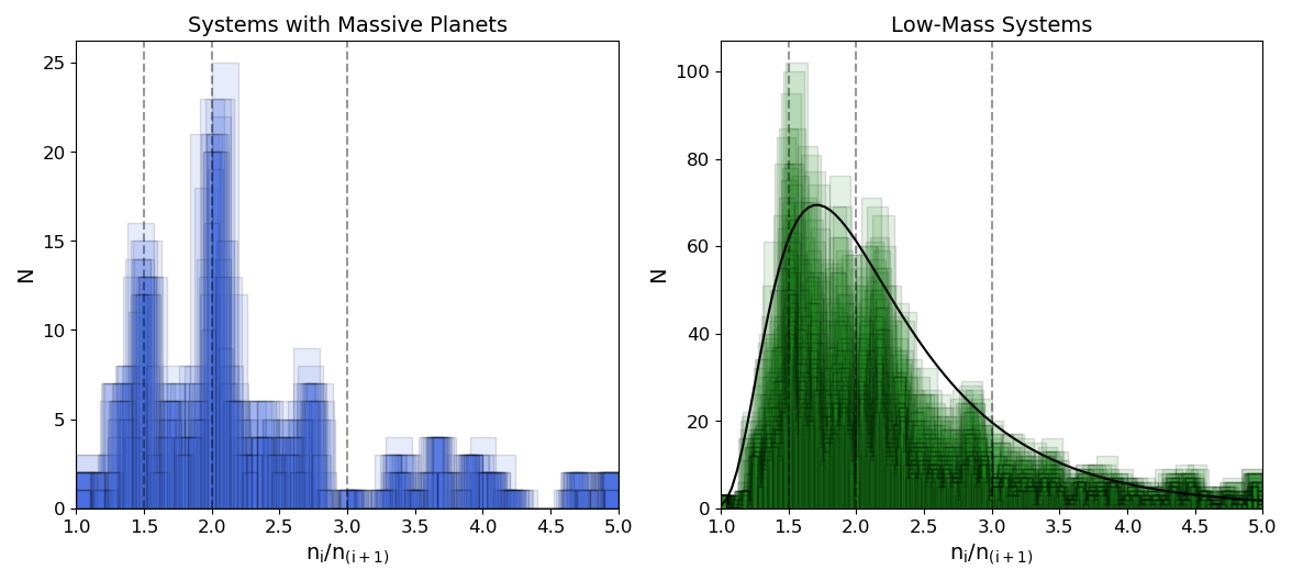
Figure 1: Distribution of mean-motion ratios $n_{i}/n_{(i+1)}$ for adjacent planetary pairs belonging to systems with at least one giant planet (left) and low-mass systems (right). The limit for the latter group was set to $20m_{\oplus}$. Main MMRs are highlighted with dashed vertical lines. An analytical lognormal approximation of the PDF for low-mass systems is shown as a black curve. Its parameters are given in equation (7).

If resonance capture were such a common outcome, or if such configurations were able to survive the dissipation of the protoplanetary disc, the distribution of mean-motion ratios $n_{i}/n_{(i+1)}$ between adjacent planets would show a strong correlation with the location of dominant commensurabilities (e.g. 2/1, 3/2). As it is well known, the real picture is more complex. Figure 1 shows the distribution of mean-motion ratios for two distinct populations of exoplanetary systems. The left-hand frame focuses only in those systems with at least one massive planet (defined as $m>100m_{\oplus}$), while the data used for the right-hand plot only includes low-mass systems where the largest known body has an estimated mass $m<20m_{\oplus}$. As mass measurements are scarce among small planets, we opted to employ the empirical mass-radius relation developed by Chen & Kipping (2017), and so these estimated masses will be prevalent in the second category. Moreover, while both limits for the planetary mass may seem a bit arbitrary, we found that the statistical analysis is fairly robust and does not change significantly when adopting other values. Data was obtained from the exoplanet.eu catalogue and, as of July 2021, included a total of 830 multi-planet systems. Of these, only 104 contain at least one massive planet while most of the rest are part of the low-mass population.

In order to avoid possible problems constructing histograms with a small number of data points, we applied a smoothing technique, which consisted in overlaying a number of histograms with different number of bins $N_{\rm bins}$ and observing the resulting structure. Robust features would be repeated in many of the individual histograms and therefore appear plotted in dark tones. Spurious features, including spikes or gaps that only appeared for specific binnings, would be plotted only a few times and thus shown in lighter shades. We considered values of $N_{\rm bins}$ between $(N_{\rm data})^{1/2}$ and $4(N_{\rm data})^{1/2}$, where $N_{\rm data}$ is the total number of bodies in each group. These limits may again be considered fairly arbitrary, but we found no significant changes in the results for other choices.

The correlation between the observed $n_{i}/n_{(i+1)}$ and mean-motion resonances shows striking differences. Large-mass systems show a significant preference for values of orbital period ratios close to the 2/1 and 3/2 commensurabilities. In particular, the peak associated to the 2/1 resonance is very conspicuous. While it is not possible to claim that most exoplanetary systems containing giant planets are located in or close to MMRs, there is a clear abundance of resonant systems. In contrast, we also find a partial gap in the vicinity of the 3/1 resonance.Previous works such as Fabrycky et al. (2014), Delisle et al. (2014) and Bailey et al. (2022) provide further insight on the impact of this MMR on the period ratio distribution.

The distribution of orbital period ratios in low-mass systems is, as expected, more blurred with no clear preference for resonant over non-resonant configurations. There appears to be a peak associated to the 3/2 resonance, but a similar one for the 2/1 commensurability is not so striking. The plot shows that most of the low-mass systems do not seem clustered around resonances.

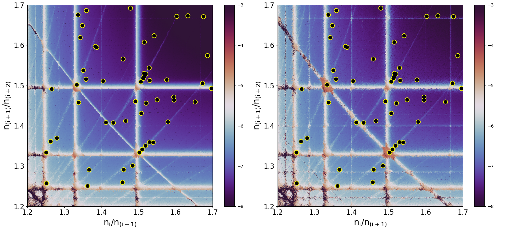
Figure 2: Both plots show the distribution of mean-motion ratios for adjacent three-planet triplets belonging to low-mass systems. Data is overlaid to ${\rm max}(\Delta a)$ dynamical maps, each constructed from N-body simulations of $1000\times 1000$ initial conditions, each integrated over a $T=10^{4}$ year timespan. In both cases planetary masses for the maps were taken equal to $m_{1}=m_{2}=m_{3}=10m_{\oplus}$. The left-hand graph was constructed with initial circular orbits, while the right-hand plot assumed $e_{i}=0.05$. All initial angles were set equal to zero, except for $\lambda_{i}$ which were taken at random for each different grid point.

This result was initially surprising because disc migration theory predicted that planet pairs would often be caught into resonances (Goldreich & Tremaine, 1980; Lee & Peale, 2002), although today we have a few hypotheses that can explain the observed difference. One of them was proposed by Goldreich & Schlichting (2014), where they have shown that eccentricity damping due to planet-disc interactions in addition to planetary migration introduces an equilibrium eccentricity which may be higher than the threshold allowed for resonant capture. This threshold is dependent on planetary mass and as such, smaller planet would be less likely to be captured. More recently, (Izidoro et al., 2017, 2021) found that many of the resonant chains formed among low-mass planets could become unstable after the dissipation of the disc, ejecting the systems from the commensurabilities and contributing to the observed low number of resonant configurations.

Notwithstanding these predictions, the last decade has seen the discovery of a number of systems locked in multi-planet MMRs. While some cases have also been detected among large-mass systems, most noticeably GJ876 and HR8799, these dynamically complex configurations appear predominantly in low-mass compact systems (e.g. Kepler-60, Kepler-80, Kepler-223, TRAPPPIST-1, TOI-178), usually close to the central star. As of today these multi-resonant systems appear as resonance chains whose building blocks are either two-planet resonances (2P-MMR) or zero-order three-planet resonances (3P-MMR). However, N-body simulations by Charalambous et al. (2018) and Petit (2021) have shown that capture in pure 3P-MMR configurations are also possible provided the migration rate is sufficiently low. We denote pure 3P-MMRs as those where no adjacent pair of planets lie in 2-planet commensurabilities.

Charalambous et al. (2018) in particular have shown cases where the end-result of migration of fictitious three-planet systems may include a combination of zero-order and/or first-order pure 3P-MMR which are distant from any two-planet commensurability. Such configurations would not be identified as resonant by studying the distribution of $n_{i}/n_{(i+1)}$ values and lead to the false impression that the system is in fact non-resonant.

Such diversity of stable multi-resonant configurations has motivated us to perform a more detailed analysis of the distribution of compact multi-planet systems, and search for any correlation with two-planet and three-planet commensurabilities. Our study is divided as follows. Section 2 discusses the known population of systems with $N\geq 3$ planets, their main dynamical features and distribution in the mean-motion ratio plane. The dynamically relevant resonant population is described in Section 3, and the main statistical analysis is shown in Section 4. Our main results are presented in Section 5 while conclusions close the paper in Section 6.

2 The Plane of Mean-Motion Ratios

2.1 Distribution of Known Systems

From the exoplanet.eu catalog of confirmed exoplanets, we selected low-mass systems with at least three planets ($N\geq 3$) and analyzed the distribution of mean-motion ratios $(n_{i}/n_{(i+1)},n_{(i+1)}/n_{(i+2)})$ for each sub-set of three adjacent planets. Thus, a 3-planet system would be characterized by a single data point in this plane, while a system with $N$ planets would yield $(N-2)$ distinct values. Since our study focuses on compact low-mass systems, we eliminated those triplets with coordinates larger than 1.7, thus removing the 2/1 MMR from the plot. The resulting distribution is shown in Figure 2 and contains a total of 57 triplets, which we will denote by the set ${\cal P}_{\rm obs}$.

The data points are overlaid on top of ${\rm max}(\Delta a)$ dynamical maps, each drawn from the numerical simulation of two different grids of $1000\times 1000$ fictitious 3-planet systems with orbits around a $1\ M_{\odot}$ star. Each simulation was performed employing a Bulirsch-Stoer integration scheme with variable time-step and precision $ll=12$ (Bulirsch & Stoer, 1966). Initial conditions for the left-hand plot correspond to circular orbits, while in the right-hand frame we opted for aligned orbits with $e_{1}=e_{2}=e_{3}=0.05$. These are close to the mean value of known eccentricities for compact systems. In both cases the planetary masses were $m_{1}=m_{2}=m_{3}=10m_{\oplus}$, while the mean longitudes where chosen randomly between zero and $2\pi$. The ${\rm max}(\Delta a)$ structure indicator was chosen for its ability to detect both 2P-MMRs and 3P-MMRs of any order.

As shown in Charalambous et al. (2018), each structure (line segment) in the dynamical maps is associated to a different mean-motion resonance. Vertical and horizontal strips correspond to two-planet commensurabilities, while intersection points between a horizontal and a vertical line mark the location of a three-planet resonance chain. Pure 3P-MMRs appear as diagonal curves stemming from bottom-left to upper-right, while an opposite trend mark 2P-MMRs involving the inner and outer member of the triplet. Some of these resonances are evident even for $e_{i}=0$ (left-hand plot) while others are only dynamically relevant for eccentric orbits (right-hand frame). However, most of the resonance network appears fairly robust and common to both maps.

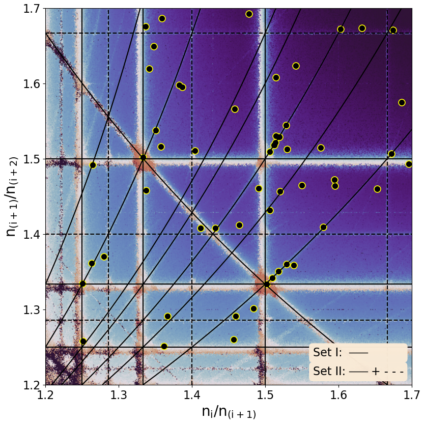
Figure 3: Overlaid to the ${\rm max}(\Delta a)$ dynamical map and distribution ${\cal P}_{\rm obs}$ of triplets, the plot shows two sets of MMRs used for the statistical analysis. Set I is indicated by continuous black lines and includes first-order 2P-MMRs and zero-order 3P-MMRs. Set II includes all of the above in addition to second-order 2P-MMRs. The complete list of resonances is summarized in Table LABEL:tab1.

2.2 The Resonance Network

The two and three-planet resonances considered in this work are summarized in Table LABEL:tab1 and drawn in Figure 3. We defined two different networks. Set I includes all first-order 2P-MMRs in the limits of the plane of mean-motion ratios (i.e. $n_{i}/n_{(i+1)}$ and $n_{(i+1)}/n_{(i+2)}$ between $1.2$ and $1.7$) as well as the most important zero-order 3P-MMRs. In addition, Set II also includes 2nd-order 2P-MMRs in the interval.The complete list is found in Table LABEL:tab1.

Three-planet resonances occur when the mean motions of a triplet of adjacent planets verify the relationship:

$$k_{i}n_{i}+k_{(i+1)}n_{(i+1)}+k_{(i+2)}n_{(i+2)}\simeq 0$$ (2)

where $k_{j}$ are non-zero integers. The sum $s=k_{i}+k_{(i+1)}+k_{(i+2)}$ indicates the order of the resonance. Zero-order commensurabilities are typically the strongest (Gallardo et al., 2016) and their libration domain is almost independent of the eccentricities (Quillen, 2011). Through N-body simulations, Charalambous et al. (2018) showed that zero and even first-order 3P-MMRs can guide the evolution of the system during migration, directing them towards a chain of resonances, where the inner and outer pair would be in a 2P-MMR each. They found that for most planet-triplets, migration would halt once the chain was reached. Furthermore, Petit (2021) showed that a system can even be trapped in a first-order resonance, although this was only achieved for controlled conditions and robustness is uncertain.

The zero-order 3P-MMRs adopted for our work were chosen according to three criteria. First, evidence of their dynamical effect must be noticeable in the ${\rm max}(\Delta a)$ map, implying at least some significant orbital excitation within the integrated time-span. Second, the resonance must lie in a region of the plane inhabited by observed triplets. Although a rigorous definition will be given later on, for now it is sufficient to say that we will avoid the sectors close to the upper left-hand and lower right-hand corners. Finally, all the chosen 3P-MMRs must have the largest values of resonance strength in the region, as estimated with the semi-numerical method of Gallardo et al. (2016). The 3P-MMRs listed in Table LABEL:tab1 satisfy these three conditions and all are of zero order.

The method for the calculation of the strength of a pure 3P-MMRs can be summarized as follows. The Hamiltonian of the system $H$ can be written as the sum of two parts $H=H_{0}-R$; the first one, $H_{0}$, is the integrable part and leads to the Keplerian motion of the planets around the central star, while $R$ groups all perturbations arising from mutual gravitational interactions between the planets: $R=R_{12}+R_{23}+R_{13}$, where

$$R_{ij}=Gm_{i}m_{j}\left(\frac{1}{|\mathbf{r_{i}-r_{j}}|}-\frac{\mathbf{r_{i}\cdot r_{j}}}{r_{j}^{3}}\right)$$ (3)

denotes the mutual perturbations between planets $m_{i}$ and $m_{j}$. For a given pure 3P-MMR, the critical angle is defined as

$$\sigma=k_{1}\lambda_{1}+k_{2}\lambda_{2}+k_{3}\lambda_{3}+\gamma$$ (4)

where $\gamma$ is a combination of the fixed longitudes of the perihelia and nodes of the three planets. Note that in the case of zero-order resonance $\sigma$ is independent of $\gamma$. The resonant disturbing function, $\mathcal{R}(\sigma)$, is constructed by an averaging method, fixing $\sigma$ and calculating the mean of $R$ but including the effects of mutual planetary perturbations. The disturbing function of a 3P-MMR is a second order function of the planetary masses, which means the calculation of $\mathcal{R}(\sigma)$ cannot be done over $R$ evaluated at the unperturbed planetary positions.

To properly calculate the mean it is necessary to take into account their mutual perturbations in the position vectors. Accordingly, given any set of the three planetary position vectors $\vec{r_{i}}$ satisfying the resonant condition given by equation 4, the mutual perturbations of the three bodies are computed and the $\Delta\vec{r_{i}}$ that they generate in a small interval $\Delta t$ are calculated. These $\Delta\vec{r_{i}}$ produce a $\Delta R$, whose mean $\mathcal{R}(\sigma)$ is then evaluated. This process involves considering a large number of the three position vectors $\vec{r_{i}}$ which are always chosen for a fixed value of $\sigma$. By changing this angle, $\mathcal{R}(\sigma)$ is numerically constructed and finally the strength is defined as the semi-amplitude of $\mathcal{R}(\sigma)$. Additional details may be found in Gallardo et al. (2016).

Table 1: Two-planet and pure zero-order 3P-MMRs considered in the resonance networks Set I and Set II. Two-planet resonances are characterized by the index array $(k_{i},k_{(i+1)})$, while 3-planet commensurabilities are defined by the array $(k_{i},k_{(i+1)},k_{(i+2)})$. The (1,0,-2) resonance is a 2-planet commensurability involving the inner and outer member of the triplet. Both sets share the same 3P-MMRs. Additionally, we will also define Set 0 as that containing the same 3-planet resonances but without any 2P-MMRs.

Set I		Set II
2P-MMR	3P-MMR	2P-MMR	3P-MMR
$(5,-4)$	$(1,-2,1)$	$(5,-4)$	$(1,-2,1)$
$(4,-3)$	$(1,-3,2)$	$(4,-3)$	$(1,-3,2)$
$(3,-2)$	$(2,-5,3)$	$(3,-2)$	$(2,-5,3)$
$(1,0,-2)$	$(3,-7,4)$	$(9,-7)$	$(3,-7,4)$
	$(4,-9,5)$	$(7,-5)$	$(4,-9,5)$
	$(3,-8,5)$	$(5,-3)$	$(3,-8,5)$
	$(5,-9,4)$	$(1,0,-2)$	$(5,-9,4)$

Figure 4 plots the location of several zero-order 3P-MMRs, whose thicknesses are drawn proportional to their strengths; the base scale chosen to allow for a visual comparison. While the strength is a function of the mutual distances, a subset of seven commensurabilities stand out over the other. These appear in blue and were chosen for our resonance network. The strongest ones appear to be those characterized by the index array $(1,-2,1)$ and $(1,-3,2)$ and house several triplets in their immediate vicinity. Other strong resonances, such as the $(1,-4,3)$ and $(3,-5,2)$ are located close to the edge of the plane and empty of known systems. Stability considerations probably favor the accumulation of data points in the general vicinity of the central area. In this region the $(2,-5,3)$ commensurability has a significant following, at least partially fueled by the $3/2$ double resonance.

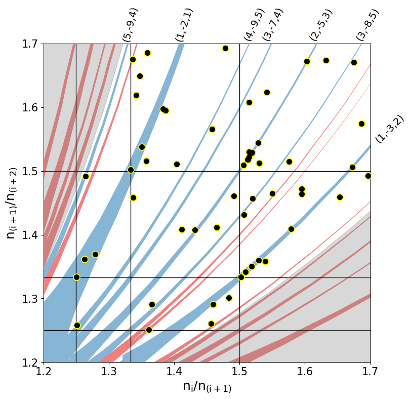
Figure 4: Location of several pure 3P-MMR in the plane of mean-motion ratios. The thickness of each curve is not related to the width of the libration domain but are proportional to the resonance strength, as estimated from Gallardo et al. (2016). Commensurabilities chosen for our statistical study are shown in blue. Black circles show the data set ${\cal P}_{\rm obs}$ of triplets from observed planetary systems.

3 Correlation Between ${\cal P}_{\rm obs}$ and the Resonance Sets

The main objective of this work is to establish whether the observed distribution of triplets ${\cal P}_{\rm obs}$ may have been determined or (at least) influenced by 2-planet and 3-planets resonances. In other words, we wish to study whether ${\cal P}_{\rm obs}$ is in some way correlated with the resonance network or if it is consistent with any random distribution. This approach is similar to that used to test the correlation of planetary pairs to 2P-MMRs; the main difference is that we must now analyze resonance structures in a two-dimensional plane instead of a one-dimensional line segment.

In order to perform these tasks, we must first define two key aspects: (i) how to measure the correlation of the observed distribution to the resonance network, and (ii) how to check whether such a value is statistically significant. Each is discussed below.

3.1 The Proximity Index

In order to measure the correlation between a given sample and the resonance web, we will define a series of proximity indices as follows:

$$I_{p}=\frac{1}{N}\sum\limits_{i=1}^{N}\Delta_{i},$$ (5)

where $N$ is the total number of triplets ($N=57$ in our study) and $\Delta_{i}$ is the linear distance from the $i$-th triplet to its nearest resonance. If every point in a given sample were to fall exactly over a resonance, then the calculation for that sample would yield $I_{p}=0$. Increasing values imply a smaller correlation between the observed distribution and the resonance web.

Two aspects must be taken into consideration. First, while the location of each resonance in the plane of mean-motion ratios is defined in terms of mean elements, the values in ${\cal P}_{\rm obs}$ are osculating and thus their short-periodic variations have not been eliminated by any averaging process. While such a transformation may be carried out, even in the case of multi-planet systems (e.g., Charalambous et al., 2018), it requires at least reasonable estimations of the planetary masses, an asset not readily available in compact systems. Fortunately, the difference in mean-motion ratios between osculating and mean elements is not significant when studying low-mass planets (e.g. $m_{i}\sim 10m_{\oplus}$), and we may avoid this step entirely.

A second issue to keep in mind is the width of each resonance. While analytical models for both 2P-MMRs and zero-order 3P-MMRs (e.g., Quillen, 2011; Hadden, 2019) are available, the libration widths are also function of the masses as well as of the eccentricities. Since the values of $e_{i}$ are also poorly delimited, we preferred to disregard the libration width of all resonances and measure the distance from the position of each triplet to the centre of the nearest MMR. While this will introduce uncertainties in the calculations, we preferred a limited but (more) robust model than a more complex version strongly dependent on unreliable parameters.

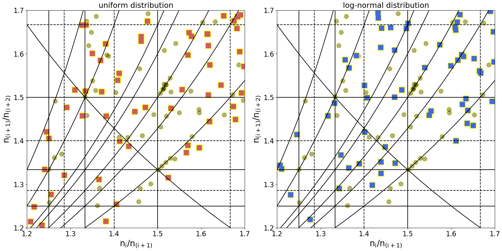
Figure 5: Squares show examples of synthetic populations of triplets in the mean-motion ratio plane. For comparison, the distribution of real planets are shown in circles. The left-hand frame was drawn assuming an uniform distribution of mean-motion ratios, while a log-normal PDF was considered in the right-hand plot.

3.2 Random Synthetic Distributions ${\cal P}_{\rm rand}$

Having calculated the values of the proximity index for the observed population, i.e. $I^{(\rm obs)}_{p}$, we must now compare it with those determined from random distributions of triplets in the plane of mean-motion ratios. We will define each ${\cal P}_{\rm rand}$ as a set of $N=57$ data points in the plane of mean-motion ratios, such that each coordinate is drawn from a given probability density function $f(x)$. We will adopt two different functional forms for the PDF. The first will be to assume a uniform distribution (i.e. flat PDF) of $x$ within the range covered by our analysis (e.g. Figure 2). While simplistic in nature, it is also the most robust and requires no ad-hoc assumptions. We will also test a second PDF that reproduces the general trend of the observed exoplanetary population. Such a ”background” PDF is estimated fitting a log-normal distribution to the mean-motion ratios of compact systems in the interval $x=n_{i}/n_{(i+1)}\in[1,4]$. This range is wider than our main region of interest (1.2-1.7), and was chosen as such in order to avoid over-fitting peaks and valleys associated with the main 2P-MMRs (namely the 2/1 and 3/2). Additionally, we tested different values for the upper bound of the interval (ranging from 3 to 5), but found no significant difference in the results. Thus, the fitting over our domain of interest seems robust under small variations of the tail of the distribution, which reassures us that, even though the falloff of planetary pairs with large period-ratios is likely biased due to observational constraints, this should have little impact on our results.

black The (3-parameter) lognormal distribution is a continuous one-dimensional distribution with the density function

$$f(x)=\begin{dcases}\frac{1}{\sqrt{2\pi}\sigma(x-x_{0})}\exp{\left[-\frac{\left[\ln{(x-x_{0})}-\mu\right]^{2}}{2\sigma^{2}}\right]},\quad{x>x_{0}}\\ \\ 0,\quad{x\leq x_{0}}\\ \end{dcases}$$ (6)

where $\mu$, $\sigma$ and $x_{0}$ are the scale, shape and location parameters, and they are such that if the random variable $X$ is lognormal, then $Y=\ln(X-x_{0})$ follows a normal distribution $Y\sim N(\mu,\sigma^{2})$ (Kozlov & Maysuradze, 2019). We adopted the values which maximized the likelihood function (MLE), giving

$$\mu=0.159\;\;\;\sigma=0.485\;\;\;x_{0}=0.804,$$ (7)

and the black curve in the right-hand frame of Figure 1 plots this function on top of the observed distribution. Except for localized peaks (associated with 2-planet MMRs) and slightly shallower valleys, the general agreement is very good.

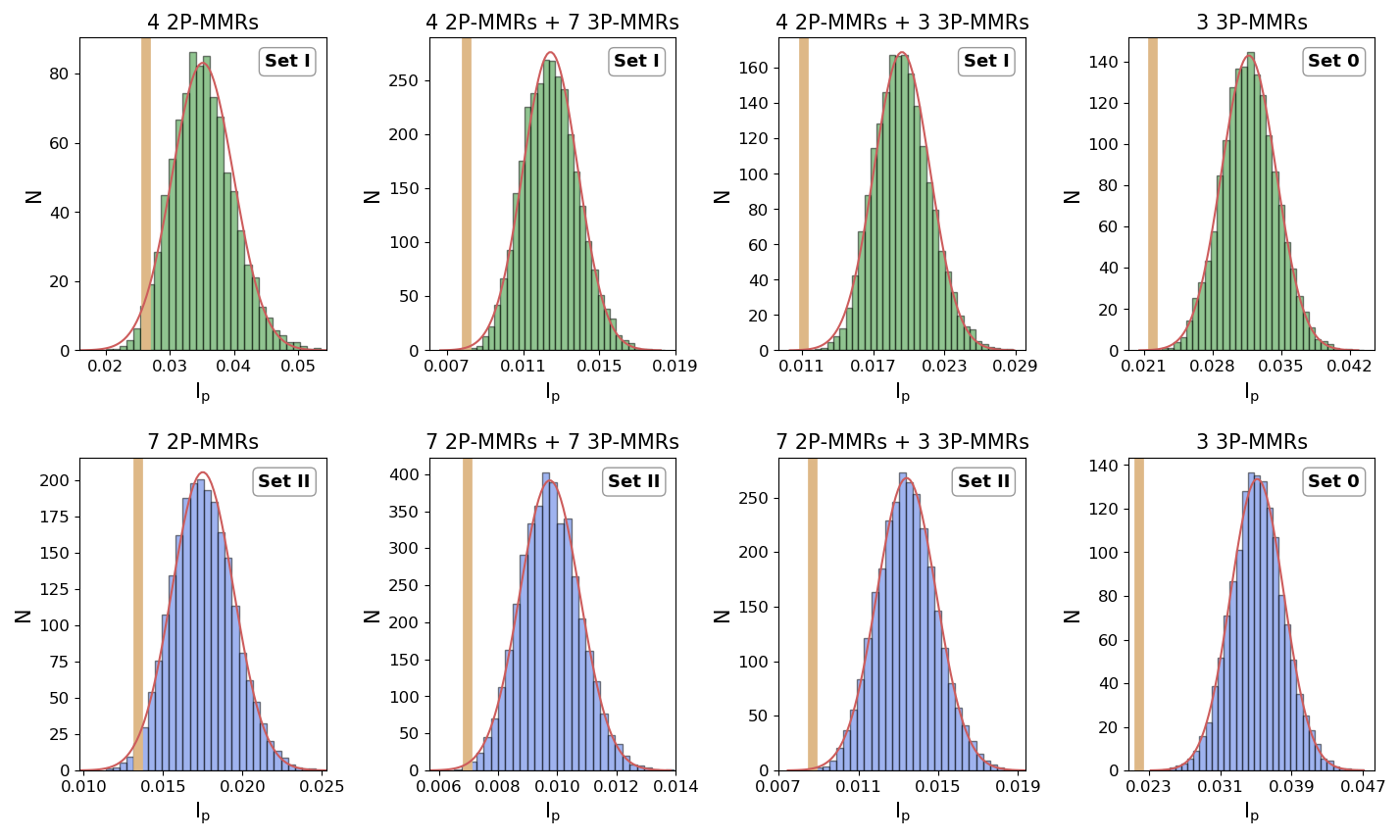
Figure 6: Histograms show the distribution of proximity indexes $I_{p}$ for series of $10^{4}$ synthetic populations of $N=57$ random triplets in the mean-motion ratio plane. The set of resonances adopted for each graph is indicated in the upper right-hand corner, and the title shows how many resonances from that set were used. Top plots assumed a uniform PDF for the random triplets, while a log-normal distribution was adopted for the bottom graphs. The value of $I_{p}$ obtained for the observed population (i.e. $I_{p}^{\rm(obs)}$) is highlighted with a broad orange vertical line.

Adopting such a smooth distribution as our null hypothesis is equivalent to assuming that the primordial formation sites of the planets were not influenced by mean-motion resonances, but primarily defined by global properties such as the surface density profile of solids and gas, disc evolution and short-term interaction between growing embryos. Thus, deviations from such a smooth and structure-less distribution, specially the overabundance of data points close to resonances, is considered a consequence of the post-formation dynamical evolution of the system. As mentioned in the introduction, the orbital distribution of systems with large-mass planets shows significant peaks that deviate from any attempt at a smooth fit and, consequently, a large number of systems are found in the vicinity of 2P-MMRs. A similar correlation is more difficult to establish for low-mass systems, thus our present study will not only include 2-planet commensurabilities but also pure 3P-MMRs.

Both expressions adopted for the synthetic PDFs (uniform and log-normal) are one-dimensional; a random point in the plane of mean-motion ratios may then be obtained applying the distribution function to each coordinate. However, as discussed previously and shown in Figure 4, the observed population of exoplanets does not cover all the plane of mean-motion ratios, and seems to avoid regions where the triplets deviate significantly from equidistant configurations. This characteristic is reminiscent of the so-called peas-in-a-pod hypothesis and has been proposed several times over the past few years (e.g. Ciardi et al., 2013; Weiss et al., 2018; Gilbert & Fabrycky, 2020). In order to incorporate this feature into our random synthetic populations, we will only consider random data points if the values of $(n_{i}/n_{(i+1)},n_{(i+1)}/n_{(i+2)})$ lie within the white region of the plot. Curiously enough, the boundaries between the populated and empty regions appear to roughly follow two different 3-planet resonances, the $(5,-9,4)$ and $(3,-10,7)$, and we will use both as a guide. Figure 5 shows examples of such synthetic populations (colored squares) overlaid to the observed exoplanetary data (circles).

4 Monte-Carlo Simulations

We generated two series of $10^{4}$ synthetic exoplanetary populations ${\cal P}_{\rm rand}$ in the plane of mean-motion ratios, each containing $N=57$ triplets; the first series was drawn from a flat PDF while the second used the log-normal distribution presented in the last section. For each random population we estimated the proximity index $I_{p}$, as defined by expression (5), to each of the resonance groups Set I and Set II. See Table LABEL:tab1 for their definitions. We added a third group (dubbed Set 0) that only contained the 7 pure 3P-MMRs but excluded all 2-planet commensurabilities. This set was used as a benchmark from which to evaluate how each type of resonance contributed to the global correlation index.

The distribution of $I_{P}$ for each series of synthetic populations is shown as histograms in Figure 6, where the label and title in each frame indicate the resonance set and how many resonances from it were used for the calculation respectively. Upper plots show results obtained from a uniform PDF in the mean-motion ratio plane; analogous runs adopting a log-normal distribution are presented in the bottom graphs. The proximity indexes $I_{p}^{\rm(obs)}$ calculated for the observed distribution of exoplanetary systems are indicated with orange vertical lines.

In all cases the spread of synthetic $I_{p}$ may be well modeled by a normal distribution with mean $\mu$ and standard deviation $\sigma$, which we overlaid as a thin red curve over each histogram; no significant difference or deviation from the bell curve is observed.

A great advantage of working with normal distributions is that it provides straightforward tests to analyze the probability of obtaining a statistic $I_{p}\leq I_{p}^{\rm(obs)}$ under the assumption that the null hypothesis is correct. For a normal distribution, this probability may be deduced by performing a $Z$-test and calculating the standard score

$$Z=\frac{\mu-I_{p}^{\rm(obs)}}{\sigma},$$ (8)

which basically measures the distances of the observed index from the most probable value, in units of the standard deviation.

Given $Z$, the probability of obtaining $|\mu-I_{p}|\geq|\mu-I_{p}^{\rm(obs)}|$ may then be estimated from the cumulative probability curve of the normal distribution, and is given by

$$P(|\mu-I_{p}|\geq|\mu-I_{p}^{\rm(obs)}|)=1-{\rm erf}\left(\frac{Z}{\sqrt{2}}\right),$$ (9)

where ${\rm erf}()$ is the error function. We can now use these statistics to analyze the results shown in Figure 6.

The two left-hand side plots compare the observed proximity index with random populations when considering only two-planet resonances. For Set I and a uniform distribution of synthetic triplets the standard score is $Z=1.84$, implying that the probability that the observed population of exoplanets satisfies the null hypothesis is $\simeq 0.07$. While relatively low, this number is not sufficiently small to strongly suggest a correlation of the planetary data with first-order 2P-MMRs. The lower left-hand plot shows similar results, this time assuming a log-normal distribution of the random populations and the Set II resonance web. As before, only 2-planet resonances are taken into account. The score of the observed distribution is now $Z=2.1$ with an associated probability of $P\simeq 0.04$. The exoplanetary population thus shows little correlation with this extended resonance set and exhibits practically the same average distance as any random distribution. This result is consistent with other statistical studies performed over the past decade, and the increase in confirmed systems does not appear to have changed the outcome.

It is interesting to note that increasing the size of the resonance set does not significantly affect the correlation with the observed distribution of triplets. We believe this is additional evidence in favor of the null hypothesis and against any significant correlation with the 2P-MMRs web. Any sufficiently large set of lines in the mean-motion ratio plane would decrease the average distance to a set of points, independently of the orientation of the lines and of the data set. As more commensurabilities are considered, the distance between any point and the web tends towards zero, and any dynamical structure that could have been inferred from limited resonance webs would be lost. In this aspect, our test proves robust and the results do not seem fooled by the number of resonances being considered.

The second-to-left plots in Figure 6 now take into account all the 2-planet and 3-planet commensurabilities that make up Set I (top) and Set II (bottom). As before, for the top frame the random populations were drawn from a uniform distribution, while a log-normal PDF was assumed for the bottom graph. Both cases show significant changes generated by the 3P-MMR web and the standard scores are now $Z=3.02$ and $Z=2.72$, respectively. These yield probabilities of $P\simeq 0.002$ for the first set, and $P\simeq 0.005$ for the second. Both values are very similar, indicating that any correlation is driven more by the web of 3-planet resonances and little affected by the 2P-MMRs and the underlying PDF for the random triplets. More importantly, results now indicate strong evidence in favor of a correlation between the observed distribution of planetary triplets and the resonance web with deviations from the norm of the order of $3\sigma$.

Next, we studied how the number of 3P-MMRs considered in the sets affects the correlation. The third column of Figure 6 shows results when reducing the number of 3P-MMRs to the three strongest resonances. As may be deduced from Figure 4, these correspond to the commensurability relations

$$\begin{split}\;\,n_{i}-2n_{(i+1)}+\;\,n_{(i+2)}&=0\\ \;n_{i}-3n_{(i+1)}+2n_{(i+2)}&=0\\ 2n_{i}-5n_{(i+1)}+3n_{(i+2)}&=0.\\ \end{split}$$ (10)

Later on we will discuss how the results vary as function of the number of 3-planet resonances. Results show an even higher degree of correlation between distribution and resonances, with now $Z=3.48$ and $Z=3.14$ for the upper and lower plots, respectively. The corresponding probabilities are $P\simeq 0.0005$ and $P\simeq 0.0016$, or about an order of magnitude lower than with the complete sets. As with the 2P-MMRs, the degree of correlation increased with a smaller resonance set, implying that most of them are probably not statistically relevant and do not contribute to the dynamical structure.

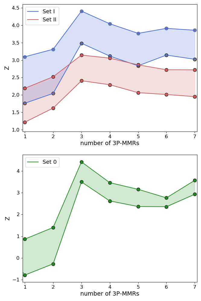
Figure 7: Variation of the standard score $Z$ as a function of the number of 3-planet resonances considered in the calculation. Upper and lower values correspond to synthetic populations following a log-normal or uniform PDF, respectively. The commensurabilities were ordered with decreasing strengths. For all resonance sets, only the first three 3P-MMRs appear relevant in establishing a correlation with the observed distribution of exoplanetary systems.

As a final test, we considered only the 3-planet resonances in the plane, thus reducing the web to Set 0. If the increase in number of 2P-MMRs from Set I to Set II decreased the correlation in all the previous calculations, we wondered whether 2-planet resonances were a relevant feature or a liability. Results are now shown in the right-hand top and bottom plots of Figure 6. The associated standard scores from the Z-test are $Z=3.50$ and $Z=4.42$, while the probabilities fall to $P\simeq 0.0004$ and $P\simeq 0.00001$. Once again, the former were obtained assuming a uniform distribution of synthetic systems in the plane, and the latter (much lower) values were calculated from a log-normal PDF.

Figure 7 analyses how the standard score varies as a function of the number of 3P-MMRs considered in the statistical test. The resonances were ordered according to their decreasing strengths, as estimated following Gallardo et al. (2016). The top frame presents results for Set I and Set II while the bottom plot focuses on Set 0. For each set, the top (bottom) values were obtained assuming a log-normal (uniform) distribution of triplets for each synthetic population. While we do not claim that the any other distribution will yield results somewhere between both limits, the shaded region helps visualize the general range of possible values. As expected, all sets show similar trends, with a sharp increase in correlation up to the third strongest resonance, whose identities were revealed in equation (10). Increasing the number of 3-planet resonances does not significantly alter the score, implying a more marginal effective correlation with the observed distribution. However, we also do not find a noticeable decrease in $Z$, so it is possible that some correlation does exist with the larger set of resonances, even if not as striking.

As a final caveat, it is important to keep in mind that we are working with low-number statistics. Even if we increase the number of synthetic populations and improve the modelization of the null hypothesis, the number of triplets per population is still small ($N=57$), a fact that undoubtedly affects the statistics. Spread over the mean-motion ratio plane, it is difficult to deduce what would have been a better representative of the primordial averaged distribution, and whether it would be better represented by a uniform or a log-normal function. The difference in standard scores $Z$ obtained for Set 0 are solely due to this issue and helps visualize the limitations of our analysis. Perhaps all we can claim at this point is that the observed distribution of planetary triplets appears significantly correlated with respect to the 3 strongest 3P-MMRs in the region. The probability that this correlation occurred by chance lies somewhere between $0.001-0.1$ per cent. No significant correlation with 2-planet resonances is observed.

5 3P-MMRs vs Double Resonances

From a simple visual analysis of the distribution of known triplets (e.g. Figure 4) it seems that a significant part of the correlation between the observed triplets and the resonance web could be caused by several multi-planet systems close to resonance chains (e.g. Kepler-80, TRAPPIST-1, etc), primarily located near coordinates $(3/2,4/3)$ and $(3/2,3/2)$. It is not clear whether these clusters effectively dominate the resonance correlation nor how other configurations contribute to the overall statistics. In this section we aim to analyze precisely this point and identify whether the correlation with 3P-MMRs is ubiquitous, or restricted to some subset of the observed population.

It is important to keep in mind that the limit between pure 3P-MMRs and double resonances is not always clear. The deviation of a given triplet from the intersection between two 2P-MMRs may be due to differential tidal effects acting over the age of the star (e.g. Papaloizou, 2015; MacDonald et al., 2016), or caused by the properties of the primordial disc that initially led to resonance capture (e.g. Charalambous et al., 2018). The magnitude of the resonance offset

$$\Delta_{(p+q)/p}=\frac{n_{i}}{n_{(i+1)}}-\frac{(p+q)}{p}$$ (11)

depends on the driving mechanism as well as on the planetary masses, eccentricities and distance from the star. Offsets caused by tidal effects lead to values that increase over time and follow the position of 3P-MMRs. Conversely, no correlation with the 3-planet resonances is expected if the offsets are generated by strong eccentricity damping during planetary migration.

Numerical simulations (e.g., Ramos et al., 2017) usually lead to values up to $\simeq 0.01$, at least for the 3/2 and 4/3 commensurabilities. This magnitude is consistent with known systems in double resonances, such as Kepler-60 (Jontof-Hutter et al., 2016) with offsets $\Delta_{(p+q)/p}\simeq 10^{-4}$ and Kepler-223 (Siegel & Fabrycky, 2021) with $\Delta_{(p+q)/p}\simeq 10^{-3}$. Only for TRAPPIST-1 (Teyssandier et al., 2022) and Kepler-60 (Jontof-Hutter et al., 2016) do 2-planet resonance offsets exceed $0.01$ and in some cases approach $0.02$. Many of the clusters observed in the mean-motion ratio plane extend far beyond these values, and it is not clear whether they actually correspond to double resonances or if they should be considered examples of true 3P-MMRs.

As a final note regarding this taxonomic issue, it is important to keep in mind that theoretical estimations of resonance offset have their limitations. Recent work on obliquity tides (e.g., Millholland & Laughlin, 2019; Millholland & Spalding, 2020) show indications that planetary spins trapped in a type-2 Cassini state could accelerate the tidal heating and orbital in-fall, at least provided adequate precession rates from external perturbers. Moreover, current estimations of tidal timescales are usually based on classical constant time lag (CTL) models (e.g. Mignard, 1979; Rodríguez et al., 2011), which are probably not the most reliable for rocky planets. No analogous studies have yet been undertaken using more sophisticated rheological models (e.g., Ferraz-Mello, 2013; Correia et al., 2014; Folonier et al., 2018), which may also change our understanding of the problem and lead to larger values of $\Delta_{(p+q)/p}$ than currently predicted.

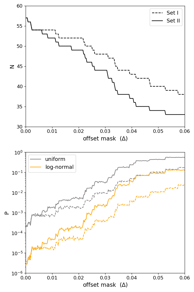
Figure 8: Top frame gives the number of bodies of the observed population that have offsets larger than $\Delta$ for every possible double resonance in each set. The bottom plot shows the variation of the probability $P$ as function of the offset mask $\Delta$. Runs adopting the resonance Set I are shown in dashed lines, while results for Set II are indicated in continuous lines.

To analyze how (near) double resonance systems may affect our statistical analysis, we repeated our Monte-Carlo simulations using both Set I and Set II but limiting the 3P-MMRs to the three strongest resonances, as described in equation (10). Because double resonances pertain to pairs of adjacent planets, we also dropped the (1,0,-2) two-planet commensurability from each set. We again generated several series of $10^{4}$ synthetic populations, adopting both a uniform and a log-normal PDF, and compared the resulting distribution of proximity indexes with that calculated with the observed population ${\cal P_{\rm obs}}$. In each run, however, the observed population was modified to exclude all triplets whose distance to the double resonances was smaller than a predefined value $\Delta$. This offset mask was varied in the range $\Delta\in[0,0.06]$, leading to a series of standard scores $Z(\Delta)$ and probabilities $P(\Delta)$.

Results are shown in Figure 8, where the top plot shows how larger offset masks remove triplets and decrease the size of the observed population. The double resonances considered for each set are those defined by every intersection of a 2P-MMR between $n_{1}$ and $n_{2}$ with another between $n_{2}$ and $n_{3}$. For Set I we considered 9 intersections including $(3/2,3/2)$, $(3/2,4/3)$, $(5/4,3/2)$, etc. For Set II the number of double resonances increased to 49, causing a significantly faster decrease in the number of surviving triplets as function of the offset mask.

The change in $P$ as a function of the offset mask is shown in the lower plot of Figure 8, where now each color corresponds to a different PDF adopted for the random populations. Recall that $P$ is an estimation of the probability that the observed distribution of triplets stems from a random population uncorrelated with the resonance web. Low values are indicative of a high correlation, suggesting that the two and three-planet resonances have influenced the distribution of planetary triplets. Values of $P$ of the order of unity point in the opposite direction.

Independently of the resonance set, the observed distribution ${\cal P}_{\rm obs}(\Delta)$ shows a high correlation with the mean-motion commensurabilities, at least for offset masks up to $\sim 0.02$. This trend is more pronounced for a log-normal distribution of random populations, and lead to very low probabilities for offsets up to $\simeq 0.04$. In all cases all evidence of correlation ceases when the population decreases by $\sim 30$ per cent, which is expected given that the ability for a statistical test to produce a low $P$ decreases with the sample size.

6 Conclusions

In this work we have presented a simple statistical analysis testing whether the distribution of known compact low-mass multi-planet systems shows significant correlation with 2-planet and 3-planet resonances. As expected from previous studies, only a faint correlation has been found with 2P-MMRs (Figure 6), and this result appears independent of the resonance set.

Conversely, we do find intriguing evidence in favor of a correlation of the observed distribution with three-planet resonances, particularly a sub-set of three commensurabilities characterized by the index $(k_{i},k_{(i+1)},k_{(i+2)})$ equal to $(1,-2,1)$, $(1,-3,2)$ and $(2,-5,3)$. These are the strongest pure 3P-MMRs in the region, a fact that increases the credibility of the result. If a set of pure 3-planet resonances were in some manner affecting the dynamics of exoplanetary systems, we would expect them to be the strongest of the set. This is indeed the case.

Among the systems which lie in 3P-MMRs, there are a striking number of them which are also close to double resonances. A possible explanation could be that these started as resonant chains which eventually proceeded to undergo detectable divergence along pure 3P-MMRs due to tidal effects (Papaloizou, 2015; Charalambous et al., 2018; Goldberg & Batygin, 2021). Isolating these systems from the population reduces the correlation with 3P-MMRs, but does not erase the statistical significance, at least for offsets of the order of those expected from tidal evolution and/or resonance capture scenarios. This seems to indicate that although resonance chains such as Kepler-60, Kepler-80, Kepler-223 and TRAPPIST-1 are an important factor, they are not dominant and the observed correlation is also fueled by systems not identified as resonance chains. Still, many of the systems showing strong correlation to pure 3P-MMRs lie relatively close to double resonances, but with large offsets of the order of $\Delta_{(p+q)/p}\sim 0.05$.

Both Charalambous et al. (2018) and Petit (2021) have shown that resonance capture in zero-order and first-order 3P-MMRs far from double resonances is possible as long as the orbital decay timescale is sufficiently long. It is thus possible that the observed correlation could have occurred during the last stages of the primordial disc when its surface density was very low and orbital excursions very limited. A similar outcome would be obtained assuming that the disc-planet interactions primarily affected the eccentricities (MacDonald & Dawson, 2018). In both cases the triplets would not have had sufficient time to evolve towards their final resting place (i.e. double resonances), leading to a distribution of systems with an excess of triplets close to but not exactly in resonance chains. Our results appear to be in favor of such a hypothetical scenario.

Finally, it is important to stress that the observed population is still small and we are working with low-number statistics. While the results are intriguing and could lead to a relevant link between pure 3-planet resonances and compact planetary systems, a much larger population is required to confirm this trend.

Data Availability

The data underlying this article are available in Github, at https://github.com/matiaspcerioni/Cerioni-Beauge-Gallardo-2022. The original data was obtained from The Exoplanet Encyclopaedia. The selected sub-samples as well as the scripts used to carry out the analysis are available in these repositories.

References

- Bailey et al. (2022) Bailey N., Gilbert G., Fabrycky D., 2022, AJ, 163, 13
- Batygin (2015) Batygin K., 2015, MNRAS, 451, 2589
- Beaugé et al. (2003) Beaugé C., Ferraz-Mello S., Michtchenko T. A., 2003, ApJ, 593, 1124
- Beaugé et al. (2006) Beaugé C., Michtchenko T. A., Ferraz-Mello S., 2006, MNRAS, 365, 1160
- Bulirsch & Stoer (1966) Bulirsch R., Stoer J., 1966, Numerische Mathematik, 8, 1