Revealing the Mechanism of Magnetic Domain Formation
by Topological Data Analysis

Abstract

Understanding pattern formation processes with long-range interactions that result in nonuniform and nonperiodic structures is important for revealing the physical properties of widely observed complex systems in nature. In many cases, pattern formation processes are measured on the basis of spatially coarse-grained features of the smallest elements, that is, the pixel space of a grayscale image. By binarizing the data using a common threshold, one can analyze such grayscale image data using geometrical features, such as the number of domains (Betti number) or domain size. Because such topological features are indicators for evaluating all regions uniformly, it is difficult to determine the nature of each region in a nonuniform structure. Moreover, binarization leads to loss of valuable information such as fluctuations in the domain. Here, we show that the analysis method based on persistent homology provides effective knowledge to understand such pattern formation processes. Specifically, we analyze the pattern formation process in ferromagnetic materials under a rapidly sweeping external magnetic field and discover not only existing types of pattern formation dynamics but also novel ones. On the basis of results of topological data analysis, we also found a candidate reduction model to describe the mechanics of these novel magnetic domain formations. The analysis procedure with persistent homology presented in this paper provides one format applicable to extracting scientific knowledge from a wide range of pattern formation processes with long-range interactions.

I Introduction

Understanding the pattern formation processes with long-range interactions that result in nonuniform and nonperiodic structures is important for revealing the physical properties of widely observed complex systems in nature, such as ferromagnetic materials, structural materials, and chemical reaction systems. In many cases, pattern formation processes are not measured on the basis of the smallest elements governing certain phenomena, such as spins, atoms, or molecules, but on the basis of spatially coarse-grained features representing a microdomain, such as mean magnetic moment, reflection ratio, or density. The pattern formation processes are often modeled mathematically on the basis of continuum approximation models, such as the time-dependent Gintzburg–Landau (TDGL) equation[1, 2], the phase-field model[3], and the reaction–diffusion model[4], which is a time evolution equation with coarse-grained microdomains as the field. Therefore, in many cases, the measurement or modeling of pattern formation dynamics can be understood to be measurement or modeling on a state space, that is, the pixel space of a grayscale image. Because such a grayscale image has a nonuniform and nonperiodic structure, existing features, such as statistical values for characterizing random phenomena or the Fourier basis for characterizing periodic structures, cannot be a state space of pattern formation dynamics. Determining how to extract the features to characterize and understand pattern formation phenomena from grayscale images is a key challenge in analyzing and understanding pattern formation processes.

An important challenge is to determine how to extract effective features from grayscale image data with the aforementioned characteristics. In conventional studies[5, 6, 7], grayscale images are often separated into domains and other regions by binarizing them using a certain threshold, and pattern formation phenomena are understood by the geometrical features of the domain structure, such as the curvature, area of the domain, and surface area. On the basis of Gauss–Bonnet theorem, the curvature is associated with a topological feature called the Euler characteristic. The area of the domain, the boundary area, and the Euler characteristic constitute the free energy that governs certain pattern formation dynamics[8]. However, when binarizing a grayscale image, information such as fluctuations in the domain may be lost. From this perspective, changes in the topological features of the domain structure at different binarization thresholds have been investigated in a previous study[9]. The study suggested that the change in the Euler characteristic is a particularly promising feature that behaves as an order parameter that characterizes a certain pattern phase. In the previous studies introduced thus far, the sum or average of the geometrical structures of all domains in the entire grayscale image is considered as a feature. In a nonuniform and nonperiodic pattern formation process, each isolated geometrical structures in the grayscale image are able to have different topological features. Therefore, to determine the properties of nonuniform and nonperiodic pattern formation processes, we need geometrical features that can represent the changes in the topological features of each isolated domain according to a threshold value.

To characterize and understand the pattern formation dynamics with long-range interaction that form nonuniform and nonperiodic structures presented as grayscale images, we employ a topological data analysis (TDA)[10, 11] method to determine the changes in the topological features of each isolated domain according to the threshold value. TDA is a general term for data analysis methods that use the concept of topology. Of the methods comprising TDA, analysis methods based on a persistent homology (PH) group[10, 11] achieve the desired feature extraction. PH is a mathematical structure that describes the birth and death of “hole” structures due to changes in a single parameter, such as the binarization threshold of grayscale images, which characterizes the geometrical structure. A hole is a ring structure in the one-dimensional case and a cavity structure in the two-dimensional case. Specifically, the number of holes corresponding to the Betti number is a homotopy invariant, that is, invariant to continuous changes of the geometrical structure, and the Betti number constitutes the Euler characteristic. PH is a topological invariant that is an extension of the Betti number to describe the birth and death of individual hole structures as the binarization threshold value increases. Thus, feature extraction based on PH can satisfy the conditions for obtaining effective features described in the previous paragraph. PH has already been applied to pattern formation data provided by grayscale images. Dłotko and Wanner applied TDA to the pattern formation dynamics of a Cahn–Hilliard system of diffusion equations and demonstrated that it is possible to estimate the total mass, which is the statistics representing the property of the pattern, and the time of a snapshot image from the extracted features[12]. Furthermore, Calcina and Gameiro applied TDA to the patterns generated using the Ginzburg–Landau equation and reported that the parameters of the simulation model can be estimated from formed patterns with high accuracy[13]. The results of these previous studies conducted to model parameter estimation indicate that the features extracted from PH retain rich information about pattern formation dynamics. Therefore, physical discovery, such as elucidating undiscovered pattern states or mechanisms of pattern formation dynamics, can be achieved by detailed analysis and interpretation of the features of pattern formation dynamics extracted from PH. From the viewpoint of obtaining novel scientific knowledge about pattern formation dynamics, PH-based methods have the following two advantages. First, PH can be inversely analyzed such that from the extracted PH structure, the representative locations of the corresponding holes in the original space[14, 15], the geometrical structure in the original space corresponding to the topological features[16], and the entire original pattern can be estimated[17]. Therefore, features obtained from PH are highly interpretable. This is useful in discussing the underlying physical mechanisms on the basis of extracted features. Second, PH satisfies the stability theorem[18], which states that when the spatial structure of data changes slightly, the PH also changes only slightly. This is a useful property of PH in discussing phase-transition-like phenomena of geometrical structures, ensuring that false detection of phase transition does not occur. Thus, a PH-based method is useful for revealing the mechanism of nonuniform and nonperiodic pattern formation processes provided as grayscale images.

The purpose of this study is to demonstrate that TDA based on PH can facilitate scientific discoveries in complex pattern formation dynamics provided as grayscale image data. We verify it by applying TDA to the process of magnetic domain pattern formation under a rapidly sweeping external magnetic field. A magnetic domain pattern, which is a spatial pattern formed by a macroscopic magnetic field, is an important feature that is closely related to the mechanism of coercivity[19]. For instance, the nonperiodic structure of magnetic domain patterns generated by spatial inhomogeneities, such as defects, impurities, steps, and strains, in the crystal structure of magnetic materials is closely related to the mechanism by which high coercivity is exhibited. As described above, the “shape” of a magnetic domain pattern is intrinsically important to the properties of ferromagnets; thus, it is important to clarify the relationship between the shape of a magnetic domain pattern and the physical properties[19]. Measurement and simulation data of magnetic domain patterns often consist of a set of average magnetic moments in a microdomain. This signifies that a grayscale pixel image is the state space in which the dynamics are discussed. In conventional analysis, the grayscale images representing the magnetic domain pattern are binarized, and geometrical features, such as the number of isolated domains or the domain length, are extracted for analysis[2, 5]. This analysis makes it possible to classify magnetic domain patterns and elucidate some of the physical mechanisms underlying their formation. The introduction of TDA using PH, which does not assume binarization, can elucidate the physical mechanism of more elaborate or extensive phenomena of magnetic domain pattern formation. In this study, we analyze time-series image data of the magnetic domain pattern formation generated by a simulation based on the TDGL equation. Because the TDGL equation is closely related to a wide class of pattern formation processes, confirming the usefulness of PH in the TDGL equation will indicate that PH is also useful for elucidating many other pattern formation dynamics.

The remainder of this paper is organized as follows. First, we describe in Sec. II the TDGL equation that simulates the process of magnetic domain pattern formation to be analyzed. Next, PH and the analytical procedure to extract new knowledge from the dynamics data of magnetic domain patterns using PH are described in Sec. III. These analysis results are presented in Secs. IV and V. Then, on the basis of novel findings of the analysis, the physical mechanisms of magnetic domain pattern formation are discussed in Sec. VI. A summary of the study is provided in Sec. VII.

II Pattern Formation Model: TDGL equation

There are a large number of physical systems that display the pattern formation process. Yttrium iron garnet (YIG) thin films, which are among the most prominent materials used in the research of spin dynamics in thin films[20], can show complex magnetic domain patterns formed by the macroscopic magnetic field. For example, depending on the sweeping rate of the external magnetic field, various nonuniform and nonperiodic patterns can be formed under a zero magnetic field. Spins in certain types of YIG thin film have a strong uniaxial anisotropy in the normal direction of the film. Therefore, the process of the magnetic domain pattern formation in the YIG thin film is sometimes modeled on the scalar field $\phi\left(\bm{r}\right):\>\mathbf{R}^{2}\rightarrow\mathbf{R}$, $\bm{r}=\left(x,y\right)$, which is composed of the average of spin-perpendicular components of small regions arranged in a lattice[1, 2]. In this continuum approximation model, the pattern formation process is described on the basis of the principle that the pattern is formed along the gradient of the energy functional composed of the mean field $\phi\left(\bm{r}\right)$. In this study, on the basis of the work of Kudo et al.[2], the time-series data of the magnetic domain pattern formation in a fast sweeping external magnetic field are generated using the TDGL equation. The variation of the pattern with the sweeping speed of the external magnetic field has been observed experimentally[2]. Understanding the pattern formation process with such complex interactions with the environment can lead to an understanding of the properties of YIG thin films in various application situations. The TDGL equation employed for pattern formation data generation is formulated as follows:

$$\frac{\partial\phi(\bm{r})}{\partial t} = -\frac{\delta H(\phi(\bm{r}))}{\delta\phi(\bm{r})},$$ (1)

$$H(\phi(\bm{r})) = H_{\rm ani}(\phi(\bm{r}))+H_{\rm J}(\phi(\bm{r}))+H_{\rm di}(\phi(\bm{r}))+H_{\rm ex}(\phi(\bm{r})),$$ (2)

where $H(\phi(\bm{r}))$ is a model of the energy function of the system. Each term is explained in the following paragraph.

$H_{\mathrm{ani}}(\phi(\bm{r}))$ is the anisotropic energy that causes the spins to align upward $\phi\left(\bm{r}\right)=1$ or downward $\phi\left(\bm{r}\right)=-1$, and it is defined as

$$H_{\rm ani}(\phi(\bm{r})) = \alpha\int d\bm{r}\lambda(\bm{r})\left(-\frac{\phi(\bm{r})^{2}}{2}+\frac{\phi(\bm{r})^{4}}{4}\right),$$ (3)

$$\lambda(\bm{r})=1+\frac{\mu(\bm{r})}{4},$$ (4)

where $\mu\left(\bm{r}\right)$ is a random variable that follows a normal distribution with mean 0 and variance $\sigma^{2}$, and $\lambda\left(\bm{r}\right)$ represents the spatial heterogeneity of the magnetic material due to defects in the crystal structure or the presence of impurities. The strength of the magnetic anisotropy is controlled by $\alpha$. $H_{\mathrm{J}}(\phi(\bm{r}))$ is the exchange interaction energy that provides the force that causes the adjacent magnetic moments $\phi\left(\bm{r}\right)$ to take the same value. It is defined as

$$H_{\rm J}(\phi(\bm{r}))=\beta\int d\bm{r}\frac{\left|\nabla\phi(\bm{r})\right|^{2}}{2}.$$ (5)

$H_{\mathrm{di}}(\phi(\bm{r}))$ is the dipole interaction energy that causes $\phi\left(\bm{r}\right)$ to take values different from those of the remote domain. It is defined as

$$H_{\rm di}(\phi(\bm{r})) = \gamma\int_{\left|\bm{r}-\bm{r}^{\prime}\right|>d}d\bm{r}d\bm{r}^{\prime}\phi(\bm{r})\phi(\bm{r}^{\prime})G(\bm{r},\bm{r}^{\prime}),$$ (6)

$$G(\bm{r},\bm{r}^{\prime})=\frac{1}{\left|\bm{r}-\bm{r}^{\prime}\right|^{3}},$$ (7)

where $d$ is the cutoff length, and set to $d=\frac{2}{\pi}$. $H_{\rm ex}(\phi(\bm{r}))$ is the energy term for the effect of the external magnetic field and is given by

$$H_{\rm ex}(\phi(\bm{r}))=-h(t)\int d\bm{r}\phi(\bm{r}).$$ (8)

The external magnetic field $h(t)$ is assumed to sweep with time $t$ as follows:

$$h(t)=\begin{cases}h_{\rm ini}-vt\>\>(t\leq\frac{h_{\rm ini}}{v})\\ 0.0\>\>(t>\frac{h_{\rm ini}}{v}).\end{cases}$$ (9)

Our simulation was assumed to run until the time at which $t=2T_{0}=\frac{2\times h_{\rm ini}}{v}$, where $T_{0}:=\frac{h_{\rm ini}}{v}$ is the time at which the external magnetic field $h(t)$ is zero.

Detailed numerical calculation methods are discussed below. By performing variational differentiation [Eq. (1)], we obtain the time derivative of $\phi(\bm{r})$ as

$$\frac{\partial\phi(\bm{r})}{\partial t}=\alpha\lambda(\bm{r})\left[\phi(\bm{r})-\phi(\bm{r})^{3}\right]+\beta\nabla^{2}\phi(\bm{r})-\gamma\int d\bm{r}^{\prime}\phi(\bm{r}^{\prime})G(\bm{r},\bm{r}^{\prime})+h(t).$$ (10)

Fourier transformation of Eq. (10) provides another perspective of the equation as follows:

$$\frac{\partial\tilde{\phi}_{\bm{k}}}{\partial t}=\alpha\left\{\tilde{\phi}(\bm{k})\star\tilde{\lambda}(\bm{k})-[(\tilde{\phi}(\bm{k})\star\tilde{\phi}(\bm{k}))\star\tilde{\phi}(\bm{k})]\star\tilde{\lambda}(\bm{k})\right\}-[\beta k^{2}-\gamma\tilde{G}({\bm{k}})]\tilde{\phi}(\bm{k})+h_{\bm{k}}\delta_{{\bm{k}},0},\>\>\>\>\>$$ (11)

where $\tilde{\phi}(\bm{k})$, $\tilde{\lambda}(\bm{k})$, and $\tilde{G}({\bm{k}})$ denote the Fourier transforms of $\phi(\bm{r})$, $\lambda(\bm{r})$, and $G(\bm{r},0)$ respectively, $\star$ denotes the convolution sum, and $k=|{\bm{k}}|$. In addition, the following conversion equation is used:

$$\int d\bm{r}\int d\bm{r}^{\prime}\phi(\bm{r}^{\prime})G(\bm{r},\bm{r}^{\prime})\exp(-i\bm{k}\cdot\bm{r})=\tilde{G}({\bm{k}})\tilde{\phi}(\bm{k}).$$ (12)

Specifically, $\tilde{G}({\bm{k}})$ is given by the following equation:

$$\tilde{G}({\bm{k}})=a_{0}-a_{1}k,$$ (13)

where $a_{0}=2\pi\int_{d}^{\infty}dr\frac{1}{r^{2}}=\frac{2\pi}{d}$ and $a_{1}=2\pi$. The time evolution [Eq. (11)] is achieved as a difference equation with a time increment of $0.1$. In the numerical calculations, the space $\bm{r}:=(x,y)$ is discretized into a mesh. Therefore, note that the distribution function of the average magnetic moment $\phi(\bm{r})$ obtained from the numerical calculations is given as $\phi(i,j),\>i,j\in\mathbf{N}$.

The TDGL equation changes the formation pattern depending on the model parameters $\alpha$, $\sigma$, $\beta$, $\gamma$, and $v$. To investigate the behavior of the TDGL equation with respect to the parameters, the linear amplification factor $\eta_{\bm{k}}$ at zero magnetization $h_{\bm{k}}=0$ of Eq. (11) was previously studied[5]. From Eq. (11), the system’s linear amplification factor is given by

$$\frac{\partial\tilde{\phi}_{\bm{k}}}{\partial t}=\eta_{\bm{k}}\tilde{\phi}_{\bm{k}},$$ (14)

$$\eta_{\bm{k}} = -(\beta k^{2}-\gamma a_{1}k+\gamma a_{0})+\alpha$$ (15)

$$= -\beta\left(k-\frac{a_{1}\gamma}{2\beta}\right)^{2}+\frac{a_{1}^{2}\gamma^{2}}{4\beta}-\gamma a_{0}+\alpha.$$ (16)

From these equations, the wavenumber component at $k=\frac{a_{1}\gamma}{2\beta}$ is the largest component, and the larger $\frac{a_{1}^{2}\gamma^{2}}{4\beta}-\gamma a_{0}+\alpha$ becomes, the broader the wavenumber component becomes. This indicates that $\frac{a_{1}\gamma}{2\beta}$ determines the rough scale of the domain structure, and $\alpha$ controls the variability of the domain size. This signifies that the geometrical structure of the magnetic domain is dominated by $\alpha$ in the range that can be explained by linear amplification without an external magnetic field. From this consideration, Kudo and Nakamura[5] fixed $\frac{a_{1}\gamma}{2\beta}$, which specifies the scale of the domain structure, to $1$ and focused on the $\alpha$ dependence of the domain structure. Kudo and Nakamura also focused on the $v$-dependence governing the nonequilibrium effects of the domain structure formation dynamics. In this study, we also focus on the change in pattern formation dynamics due to $\alpha$ and $v$. Specifically, $v$ is set as $0.0001\leq v\leq 0.01$ and $\alpha$ is set as $1.0\leq\alpha\leq 4.0$ at uniformly random or equal intervals depending on the purpose of each analysis. Other parameters are set according to Ref. [5] (Table 1).

Table 1: Parameters of TDGL equation.

$\alpha$	$\beta$	$\gamma$	$h_{\rm ini}$	$v$	$d$	$\sigma$	Lattice size
1.0–4.0	2.0	$\frac{2.0}{\pi}$	1.5	0.0001–0.01	$\frac{\pi}{2}$	0.3	512 $\times$ 512 (periodic boundary)

III Analysis methods

III.1 Topological data analysis

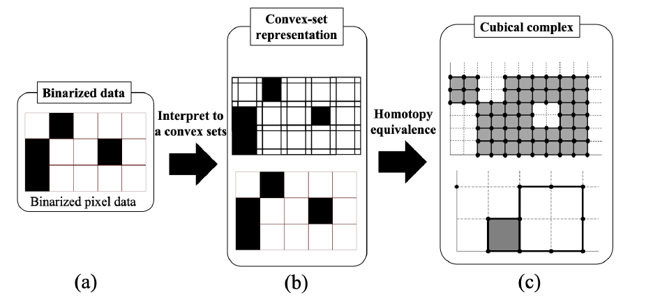
Figure 1: Two examples of converting data to a cubical complex (see Appendix A). (a) Binarized pixel image data. (b) Two ways of representation of the data as a set of closed convex sets (quadrilaterals). (c) Two ways of representation of the set of closed convex sets as a cubical complex.

A PH group represents a figure as a set of creation and annihilation of hole structures depending on a single parameter. Note that the sequence of geometric elements of the figure which is created according to an increase of a single parameter needs to form a monotonically increasing sequence. As an example, we consider the PH group of a two-dimensional grayscale image $G:=\{G(i,j)\in[0,1]\mid\>1\leq i\leq d_{x},1\leq j\leq d_{y}\}$ composed of $d_{x}\times d_{y}$ pixels, where $\>G(i,j):\mathbf{N}^{2}\rightarrow[0,1],\>i=1,2\cdots d_{x},\>j=1,2\cdots d_{y}$. To compute the PH group, the domain structure of the pixel image data must be re-expressed as a set of closed convex sets, such as a rectangle [Figs. 1(a) and (b)]. If we set the domain as an area that takes a large value, the domain area is given as the set of pixels that are greater than a certain threshold $t$ (superlevel set) as follows:

$$\{G_{i,j}\mid G(i,j)\geq t,1\leq i\leq d_{x},1\leq j\leq d_{y},\}.$$ (17)

By representing one pixel $G(i,j)$ in domain area as a closed convex set $s_{ij}$ [Fig. 1 (b)], we obtain set of closed convex sets representing domain areas,

$$S_{t}:=\{s_{ij}\mid G(i,j)\geq t,1\leq i\leq d_{x},1\leq j\leq d_{y},\}.$$ (18)

By reducing the parameter $t$ from 1 to 0, we find that the level set of the grayscale image $S_{t}$ constructs an increasing sequence $\mathbf{S}$ of its geometric elements:

$$\mathbf{S}:S_{t_{1}}\subset S_{t_{2}}\cdots\subset S_{t_{n_{\Theta}}},$$ (19)

where $1\geq t_{k}>t_{k+1}\geq 0$ and $t_{n_{\Theta}}$ is a threshold at which all pixels become larger than it. Here, the threshold value $t$ is replaced by $t^{\prime}=1-t$ to let the threshold value correspond to a single parameter that increases corresponding to the increasing sequence of its geometric elements. When a grayscale image $G$ is binarized into 0 and 1 at a certain threshold $t^{\prime}$, if 1 is the domain, the 0 region surrounded by 1 is the hole. Note that holes in zero dimensions represent a connected component, holes in one dimension represent a ring, and holes in two dimensions represent a cavity. For a two-dimensional pixel image, zero-dimensional and one-dimensional holes are considered.

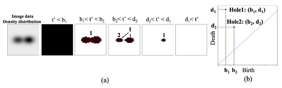
Figure 2: Grayscale image data and PH. (a) One-parameter (threshold) change in the figure structure and (b) the corresponding persistence diagram (PD).

As an example of how the hole structure changes with a single parameter $t^{\prime}$, we consider a grayscale image illustrated in Fig. 2(a). In this grayscale image, at $t^{\prime}=0$, the entire pixel image is a nondomain region. As $t^{\prime}$ increases, domain regions emerge and are connected to each other; then, they generate one large hole at $t^{\prime}=b_{1}$ [see Hole 1 in Fig. 2(a)]. As $t^{\prime}$ increases further, the large hole is divided into two holes in a domain at $t^{\prime}=b_{2}$ [see Hole 2 in Fig. 2(a)]. When $t^{\prime}$ is further increased, one of the holes is filled and disappears at $t^{\prime}=d_{2}$. The other hole is also filled and disappears at $t^{\prime}=d_{1}$. Note that the death of a hole signifies that the entire hole area at the birth of the hole is filled. This implies that even if the hole splits into two owing to an increase in $t^{\prime}$, the identity is not inherited by one hole, but by both hole regions [see Hole 1 in Fig. 2(a)]. In addition, the remaining hole birth–death structures that cannot be expressed by the birth–death structure of the first hole are treated as another birth–death structure of the second hole [see Hole 2 in Fig. 2(a)]. By defining the death and birth of a hole in this way, we can uniquely determine the set of birth–death intervals of the holes (persistent intervals) $I$ defined below for an increasing sequence of geometric elements of the figure:

$$I = \{I_{k}\mid 1\leq k\leq N_{\rm hole}\},$$ (20)

$$I_{k} := \begin{cases}[b_{k},d_{k}),\>\>{\rm for}\>\>k=1\cdots u&\\ [b_{k},\Theta],\>\>{\rm for}\>\>k=u\cdots N_{\rm hole}&\end{cases},$$ (21)

where $N_{\rm hole}$ is the number of holes, $I_{k}$ is the persistent interval of each hole, $\Theta$ is the threshold (saturation time) at which the domain structure does not change even if the threshold is changed further, and $u$ is the number of holes whose death threshold is less than $\Theta$. An example of a hole that disappears at saturation time is a hole in a torus structure that originates from periodic boundary conditions of numerical simulation. PH groups have been demonstrated to have isomorphic representations that are uniquely determined by specifying $I$[21]. A diagram of a persistent interval $I$ with the horizontal axis as the threshold $b_{k}$ at which a $l$-dimensional hole is generated and the vertical axis as the threshold $d_{k}$ at which the $l$-dimensional hole disappears is defined below as persistence diagram (PD):

$$PD_{l}(\mathbf{K})=\{(b_{k},d_{k})\in\mathbf{R}^{2}\mid k=1,2\cdots N_{\rm hole}\}.$$ (22)

where $\mathbf{K}$ is the increasing sequence of cubical complex [Fig. 1(c)] corresponding to the increasing sequence of closed convex sets $\mathbf{S}$ (see Appendix A for more detail). The cubical complex is a figure structure formed by pasting together d-dimensional rectangles, such as points, lines, and rectangles. The $(b_{k},d_{k})$ corresponding to one hole on the PD is also called a generator of the PD, which is referred to simply as “generator” in this paper. PH groups are often expressed as this PD [Fig. 2(b)]. In this study, we perform feature extraction from the PD. Note that the obtained PH group changes depending on how to define the closed convex set $s_{ij}$, it is shown in the upper panels and the lower panels of Figs. 1 (b) and (c). For more information, see Appendix A.

For the magnetic domain pattern $\phi\left(\bm{r}\right)$ obtained using the TDGL equation, the PD is calculated with the binarization threshold $t^{\prime}$ as one parameter similarly to grayscale image data. The PDs of $l=0,1$ are calculated from the magnetic domain pattern, which is two-dimensional image data. In this study, we focus on the PD of $l=1$, which expresses the birth–death pair of a one-dimensional hole (ring) structure. Note that, as in the method described for grayscale images, we define a domain as a region that is above a threshold value. To apply machine learning analysis, the obtained $PD_{1}(\mathbf{K})$ [Eq. (22)], which is the point cloud representing the birth–death pairs, is converted into vector data. In this study, we vectorize $PD_{1}(\mathbf{K})$ on the basis of the persistent image method[22]. In this method, the histogram of the point cloud $PD_{1}(\mathbf{K})$ is calculated first.

$$h\left(x,y;PD_{1}(\mathbf{K}),\sigma\right)=\sum_{i=1}^{N_{\rm hole}}\frac{1}{2\pi\sigma}\exp\left\{-\frac{1}{4\sigma^{2}}\left[(x-b_{i})^{2}+(y-d_{i})^{2}\right]\right\}$$ (23)

We do not correct the histogram to reduce the intensity of short-lived holes corresponding to noisy structures, which is often performed in the persistent image method. This is because in this study, we also focus on the information of intradomain fluctuations corresponding to noisy structures. The number density is extracted from the histogram function into a $d\times d$ grid of $\{x_{i},y_{j}\}_{i,j}$, and the vector data are generated as follows:

$${\bf v}(h\left(\>\cdot\>,\>\cdot\>;PD_{1}(\mathbf{K}),\sigma\right);d)=\left(h(x_{1},y_{1}),h(x_{2},y_{1}),\dots,h(x_{d},y_{d})\right).$$ (24)

The kernel width $\sigma$ of the Gaussian kernel used for histogramming and the number of grids $d$ for vectorization were set as hyperparameters. These hyperparameters are set to minimize the validation error of the regression model $F(\>\cdot\>;\bm{\Theta})$ given by the following equation for the inverse estimation of model parameters described in Sec. IV:

$$E(\bm{\Theta},\sigma,d)=\frac{1}{2N_{\rm val}}\sum_{\{{\bf v}_{i}(\sigma,d),y_{i}\}\in D_{\rm val}}\left[F({\bf v}_{i}(\sigma,d);\bm{\Theta})-y_{i}\right]^{2},$$ (25)

where ${\bf v}_{i}(\sigma,d)$ is the vectorized data of the PD for a certain magnetic domain pattern data $i$, $y$ represents the model parameters of the TDGL equation that we want to predict, $D_{\rm val}$ is the validation dataset that is not used for training the regression model, and $\bm{\Theta}$ is the model parameter of the regression model. The optimized vector data are used as they are to create a classification diagram by clustering the magnetic domain pattern. This is based on the idea that a hyperparameter that effectively predicts physical properties that are important for a phenomenon can effectively extract information about the target.

III.2 Analysis procedure to reveal the mechanisms of pattern formation dynamics

To understand the mechanism of the process of magnetic domain pattern formation, it is appropriate to analyze a snapshot taken at a characteristic time representative of the system. Pattern formation processes with long-range interactions have a complex multivalley energy landscape. Therefore, depending on the initial state of the system or the interaction process with the environment, the system should reach different metastable states or saddle points. In this study, the initial state of the system was set to be the same in all simulations. The system is expected to reach different local minima or saddle points depending on the sweep rate $v$ of the external magnetic field. Therefore, the snapshot at $t=2T_{0}$, which is the time when the system behaves with a certain degree of stability after the sweep of the external magnetic field ends, was chosen for analysis. By analyzing the snapshot at $t=2T_{0}$, we verify that the PD retains sufficient information about the system, and we search for novel insights into the relationship between the geometric features of the magnetic domain and the physical properties of the system.

The physical mechanism underlying the novel findings obtained from the analysis of the snapshot at $t=2T_{0}$ could be understood by analyzing the formation process of the relevant magnetic domain structure. For this purpose, we calculated the PD corresponding to each snapshot at each time of the pattern formation process and searched for the time transition of the geometric structure associated with the novel knowledge obtained by analyzing the snapshot at $t=2T_{0}$. By investigating the correspondence between the obtained time transition properties of the geometric structure and the energy model of the TDGL equation, we discover the mechanism underlying the discovered phenomenon.

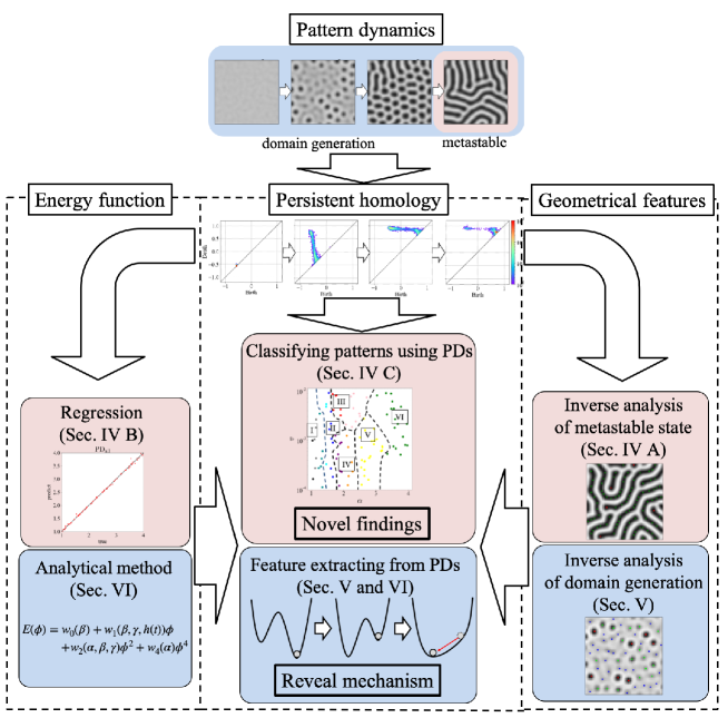
Figure 3: Analysis procedure to reveal the mechanisms of pattern formation dynamics.

The analysis procedures described above and the corresponding sections are summarized in Fig 3.

IV Analysis of snapshot at $t=2T_{0}$

From the results of TDA of the stable-state magnetic domain pattern, we identified the geometrical structure that characterizes the dominant parameters $\alpha$ and $v$ of the TDGL equation, and we search for novel insights into the relationship between the geometric features of the geometrical structure of the magnetic domain and the physical properties of the system. For this purpose, we first used the inverse analysis method of PH[14, 15], which we explain later, to obtain a geometrical interpretation of the characteristic structure of generator distribution in the PD of the magnetic domain pattern. Next, we conducted regression analysis to elucidate the correspondence of the dominant parameters $\alpha$ and $v$ of the TDGL equation to the geometrical structure obtained from PD. Furthermore, by utilizing clustering methods to create a pattern classification diagram in the $\alpha$–$v$ plane, we were able to precisely interpret the geometry extracted from PD. In addition to this verification, novel physical findings were explored. The results of these analyses are described below.

IV.1 PD and corresponding geometrical features

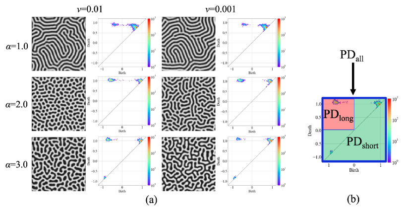
Figure 4: (a) Magnetic domain pattern (first and third columns) and corresponding PDs (second and fourth columns) for the magnetic domain patterns at $t=2T_{0}$ for each of $\alpha$ and $v$. (b) Definitions of regions of PD: ${\rm PD_{all}}$, ${\rm PD_{long}}$, and ${\rm PD_{short}}$.

We used the inverse analysis method[14, 15] to geometrically interpret the characteristic structure of generator distribution in the PD of the magnetic domain pattern. We performed numerical simulations based on the TDGL equation for $\alpha=\{1.0,2.0,3.0\}$ and $v=\{0.01,0.001\}$, and we obtained the magnetic domain pattern as shown in the first and third columns of Fig. 4(a) at $t=2T_{0}$. The PDs corresponding to each magnetic domain pattern are shown as the second and fourth columns in Fig. 4(a). From this figure, we can see that PDs tend to have a different distribution structure depending on $\alpha$ and $v$. It is also observed in this figure that the generators are concentrated in three locations on the PD: lower left, upper left, and upper right, regardless of $\alpha$ and $v$. The generator around the diagonal line of the PD represents a short-life hole, whereas the generators far from the diagonal line represent long-life holes.

By inverse analysis[14, 15], we investigated the geometrical structure of the magnetic domain pattern corresponding to the long-life region ${\rm PD_{long}}$ and the short-life region ${\rm PD_{short}}$ [Fig. 4(b)]. We extracted the last annihilating cube in one cubical complex, which disappears following the threshold value changes, as the approximate location of the hole corresponding to a certain generator. Hereinafter, we call the cube a “death cube”. As a result, it is found that the death cubes of the long-life region ${\rm PD_{long}}$ are the pixels with the smallest magnetic moment in the same magnetic domain, and the death cubes of the short-life region ${\rm PD_{short}}$ are the pixels at a relatively small peak existing in the magnetic domain. It means that the long-lifetime region ${\rm PD_{long}}$ represents the magnetic domain structure, and the short-lifetime region ${\rm PD_{short}}$ represents fluctuations in the inverse domain of $\phi<0$ (Fig. 5). A similar inverse analysis shows that the short-life generators distributed in the lower left of the PD, as seen in Fig. 4 at $\alpha=3.0$, correspond to fluctuations in the positive magnetic domain of $\phi>0$.

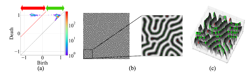
Figure 5: Correspondence between the distribution structure of the generators in the PD and the magnetic domain pattern. (a) PD of the magnetic domain pattern with $\alpha=1.5$, $v=0.01$ at $t=2T_{0}$. The long-life region of PD is shown in red, and the short-life region of PD is shown in green. (b) Magnetic domain pattern and its enlarged image. Red dots in the enlarged image represent the positions of the death cubes corresponding to the long-life region of the PD, whereas green dots represent the positions of death cubes corresponding to the short-life region of the PD. (c) Three-dimensional representation of the magnetic domain pattern, where red and green dots represent the locations of long-life and short-life death cubes, respectively. The HomCloud library[23] was used to extract the positions of the death cubes. The method to construct convex closed sets to estimate the positions of the death cubes using the HomCloud library is given in Appendix A.

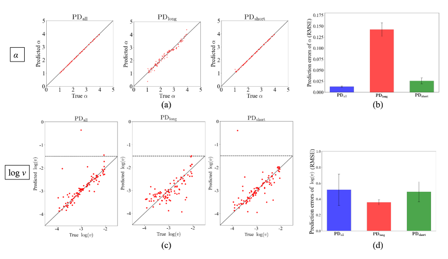
Figure 6: (a) Regression results for $\alpha$. The horizontal axis is the true value of $\alpha$ used for the TDGL simulation, whereas the vertical axis is the prediction value estimated by the outer loop of nested cross-validation. (b) Prediction error (root mean squared error) of the constructed regression model for $\alpha$ when Ridge regression is applied with vectorized ${\rm PD}_{\rm all}$, ${\rm PD}_{\rm long}$, and ${\rm PD}_{\rm short}$ as inputs. (c) Regression results for $\log\>v$. The horizontal axis is the true value of $\alpha$ used for the TDGL simulation, whereas the vertical axis is the prediction value estimated on the outer loop of nested cross-validation. (d) Prediction error (root mean squared error) of the constructed regression model for $\log\>v$ when Ridge regression is applied with vectorized ${\rm PD}_{\rm all}$, ${\rm PD}_{\rm long}$, and ${\rm PD}_{\rm short}$ as inputs.

IV.2 Regression analysis of PDs

We conducted regression analysis to verify whether the PD retains sufficient information to estimate the dominant parameters $\alpha$ and $v$ of the system. For regression analysis, $\alpha$ and $\log v$ were generated uniformly at random in the range $\alpha=[1.0,5.0]$, $\log\>v=[-4,-2]$, and the TDGL equation was run numerically under these parameters until $t=2T_{0}$. Of these, 96 sets of simulation data $\{K_{k}(i,j),\alpha_{k},v_{k}\}_{k=1}^{N=96}$ were analyzed, where the numerical calculation errors did not diverge owing to rapid changes in the magnetic moments $\phi\left(\bm{r}\right)$ during the formation process. We apply multiple regression analysis to the data set $\{{\bf v}_{i}(\sigma,d),\alpha_{i}\}_{i=1}^{96}$ and $\{{\bf v}_{i}(\sigma,d),\log\>v_{i}\}_{i=1}^{96}$, where ${\bf v}_{i}(\sigma,d)$ is vectorized PDs generated by the procedure in Sec. III.1. For the multiple regression analysis, we performed Ridge regression using the error function.

$$E = \frac{1}{2N_{\rm train}}\sum_{i=1}^{N_{\rm train}}\left[F({\bf v}_{i}(\sigma,d);\bm{w})-y_{i}\right]^{2}+\lambda\mathbf{w}^{T}\mathbf{w},$$ (26)

$$y_{i}\in\left\{\alpha_{i},\log\>v_{i}\right\},$$ (27)

where $F(\>\cdot\>;\bm{w})$ is the linear regression function $\mathbf{R}^{d^{2}}\rightarrow\mathbf{R}$, $\mathbf{w}:=(w_{1},w_{2}\cdots w_{d^{2}})$ is the regression coefficient, $\lambda$ is the regularization parameter, and $N_{\rm train}$ is the number of training data. $\lambda$, the kernel width $\sigma$, and the number of grids $d$ in vectorizing the PD are hyperparameters of this regression model. In this study, we applied the nested cross-validation framework[24] to estimate hyperparameters and prediction errors from a small amount of data. Nested cross-validation is often used to train a model in which hyperparameters should also be optimized. Nested cross-validation estimates the generalization error of the underlying model and its hyperparameter on the basis of two cross-validations in a nested relationship (see Appendix B). The regression model is trained using the hyperparameters selected in the innerloop of nested cross-validation, and the prediction error of the model is estimated using the outerloop. By plotting together the test predictions $y_{i}$ for all outer-loop folds, we obtain prediction values of all data in $\{{\bf v}_{i}(\sigma,d),y_{i}\}_{i=1}^{96}$ (Fig. 6). ${\rm PD}_{\rm all}$ in Fig. 6(a) shows the $\alpha$ estimation and ${\rm PD}_{\rm all}$ in Fig. 6(c) shows the $\log\>v$ estimation. This regression result confirms that a high prediction accuracy of $\alpha$ [${\rm PD}_{\rm all}$ in Fig. 6(a)] and accuracy of $\log\>v$ to some extent [${\rm PD}_{\rm all}$ in Fig. 6(c)] can be obtained. When we employed all the regions of PD, ${\rm PD}_{\rm all}$, for estimating $\alpha$, its root mean squared error (RMSE) was about 0.001 [${\rm PD}_{\rm all}$ in Fig. 6(b)], and its R-squared value was greater than 0.99. Since the range for $\alpha$ is 1–4, this RMSE is very small. The estimation accuracy of $\log\>v$ was not as high as that of $\alpha$. We statistically determined whether the linear regression can extract geometric information from the PD, which would allow us to estimate $\log\>v$. By performing the permutation test, we confirmed that the accuracy of the estimation of $\log\>v$ is significantly higher than that of the null model (Appendix C). As described in Introduction, it has been reported that a high $\alpha$ regression performance can be obtained using TDA in a simple Ginzburg–Landau equation whose energy model does not have a time-varying external magnetic field[13]. The facts that a similarly high performance was obtained for the system of energy functions with a time-dependent external magnetic field targeted in this study and that the parameter $v$ governing its time-varying term was predicted to some extent support the effectiveness of TDA for the analysis of complex nonequilibrium pattern formation dynamics.

Here, we try to elucidate the correspondence of the dominant parameters $\alpha$ and $v$ to the geometrical structure of magnetic domains obtained from the inverse analysis of PD. We define the two characteristic distribution structures of PD obtained by the inverse analysis: the long-life region ${\rm PD_{long}}$, which describes the topological structure of the magnetic domain, and the short-life region ${\rm PD_{short}}$, which corresponds to the internal structure of the magnetic domain. We elucidate the relationship between these characteristics and dominant parameters. For this purpose, a regression model predicting $\alpha$ and $\log\>v$ with the overall regions ${\rm PD_{all}}$, the long-life region ${\rm PD_{long}}$, and the short-life region ${\rm PD_{short}}$ as explanatory variables was constructed using the procedure described above. As a result, in the estimation of $\alpha$, ${\rm PD_{short}}$ achieved a high prediction performance similarly to ${\rm PD_{all}}$, whereas ${\rm PD_{long}}$ has a relatively low estimation accuracy [Fig. 6(b)]. In the estimation of $\log\>v$, we did not see a clear difference between characteristics as seen in $\alpha$ [Fig. 6(d)]. These results suggest that not only the geometric features of the binarized magnetic domains, as has been used in previous research, but also the contour features of the magnetic domains, such as fluctuations in the domain, contain information about the physical mechanisms of the system.

The result that the RMSE of ${\rm PD}_{\rm short}$ was smaller than that of ${\rm PD}_{\rm long}$ in estimating $\alpha$ suggests that ${\rm PD}_{\rm short}$ has more useful information than ${\rm PD}_{\rm long}$ for the estimation of $\alpha$. On the other hand, in the estimation of $\log\>v$, the RMSE of ${\rm PD}_{\rm long}$ was not larger than those of other regions, which indicates that ${\rm PD}_{\rm long}$ retains useful information for the estimation of $v$. These results suggests that $\alpha$, which dominates the anisotropic energy, contributes to the formation of the local structure of magnetic domains, and $v$, which dominates the nonequilibrium process, contributes to the formation of the global structure of magnetic domains. These are consistent with a previous study by Kudo and coworkers in which $\alpha$ dominates the variation in the periodic structure of the spatial magnetic distribution[2] whereas $v$ dominates the domain size[5]. These results can be obtained because in TDA, $\phi\left(\bm{r}\right)$ is treated as a continuous value.

IV.3 Classifying patterns based on PDs

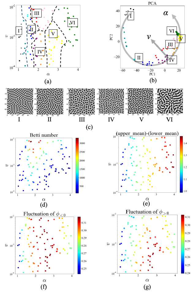
Figure 7: Results of classification of the magnetic domain patterns using feature data $\{{\bf v}_{i}(\sigma,d)\}_{i=1}^{96}$ [Eq. 24] extracted from the PD. (a) Classification results were obtained by K-means clustering. The horizontal axis represents $\alpha$ and the vertical axis represents $v$ of the TDGL equation. (b) Results of PCA of $\{{\bf v}_{i}(\sigma,d)\}_{i=1}^{96}$. The horizontal axis represents the principal component with the largest eigenvalue, whereas the vertical axis represents the principal component with the second largest eigenvalue. (c) Magnetic domain patterns at $t=2T_{0}$ roughly corresponding to points I–VI in figures (a) and (b). (d) Distribution of the Betti number of the domain structure binarized using $\phi=0$ at $t=2T_{0}$. (e) Distribution of differentiation between the mean magnetic moment of the positive magnetic domain and negative magnetic domain at $t=2T_{0}$. (f) Distribution of the standard deviation of the magnetic moment of the inverse magnetic domain at $t=2T_{0}$. (g) Distribution of the standard deviation of the magnetic moment of the positive magnetic domain at $t=2T_{0}$.

Magnetic domain patterns were classified on the basis of PD, and the relationship between the characteristics representing each classification class and the dominant factors $\alpha$ and $v$ of the system was examined. We applied the K-means clustering method[25, 26, 27] to the vectorized data $\{{\bf v}_{i}(\sigma_{\rm opt},d_{\rm opt})\}_{i=1}^{96}$ of PDs to find pattern classes with similar properties. The vectorized parameters $\sigma_{\rm opt}$ and $d_{\rm opt}$ of PDs were selected on the basis of regression analysis results in the previous paragraph. The classification is based on the Euclidean distance defined for any two vectors ${\bf v}_{i_{1}}(\sigma_{\rm opt},d_{\rm opt})$ and ${\bf v}_{i_{2}}(\sigma_{\rm opt},d_{\rm opt})$ taken from the vectorized data $\{{\bf v}_{i}(\sigma_{\rm opt},d_{\rm opt})\}_{i=1}^{96}$:

$$\sqrt{\left[{\bf v}_{i_{1}}(\sigma_{\rm opt},d_{\rm opt})-{\bf v}_{i_{2}}(\sigma_{\rm opt},d_{\rm opt})\right]^{T}\left[{\bf v}_{i_{1}}(\sigma_{\rm opt},d_{\rm opt})-{\bf v}_{i_{2}}(\sigma_{\rm opt},d_{\rm opt})\right]}.$$ (28)

The optimal hyperparameters $\sigma_{\rm opt}$ and $d_{\rm opt}$ take different values between the regression analysis results of $\alpha$ and $v$. We performed clustering analysis for each hyperparameter. Since the results were almost identical, we only show clustering results using hyperparameters optimized by regression analysis of $\alpha$ (see Appendix D for clustering analysis based on regression analysis of $v$). The number of clusters K was determined using the elbow method[28], which employs the sum of squared distances of samples to their closest cluster center as the criteria of a good cluster. As a result, $K=11$ was chosen. The classification result is shown in Fig. 7(a). Fig. 7(a) takes $\alpha$ as the horizontal axis and $v$ as the vertical axis, and each point in the figure corresponds to the magnetic domain pattern at $t=2T_{0}$ obtained by numerical simulation using each parameter. The different colors of points in Fig. 7(a) represent the different clusters. From this figure, it was found that the clusters obtained on the basis of PDs also have a cluster structure in the dominant parameters $\alpha$–$v$ space. This supports the results of regression analysis that the geometric structure obtained from the PDs is strongly related to $\alpha$ and $v$. These classification results could be independent of the clustering method (see Appendix C). Fig. 7(b) shows the distribution of the vectorized PDs data $\{{\bf v}_{i}(\sigma_{\rm opt},d_{\rm opt})\}_{i=1}^{96}$ reduced to two dimensions by principal component analysis (PCA). The cumulative contribution of the two principal components comprising the reduced space was more than 85%. This confirms that the information of $\alpha$ and $v$ is smoothly embedded in the principal component space of the features. The increase in $\alpha$ appears to correspond to the clockwise direction in this reduced space, and the increase in $v$ appears to correspond to the direction of the center of the circle. Thus, the feature space obtained from the PD appears to retain significant information about the physical property of the system.

The physical meaning of the obtained cluster structure is interpreted by defining some feature values obtained from regression analysis results. For later explanation, we define six parameter regions delineated by dotted lines in Fig. 7(a). Examples of magnetic domain patterns I–VI for each parameter region are illustrated in Fig. 7(c). Pattern III has an sea-island structure described in previous studies[5, 2], and patterns V and VI have a labyrinthine structure. Pattern I also has a labyrinthine structure, and patterns II and IV have a mixture of sea-island and labyrinthine structures. From the knowledge of the relationship between PD and magnetic domain patterns obtained from the inverse analysis of PD and the regression analysis of ${\rm PD_{all}}$, ${\rm PD_{long}}$, and ${\rm PD_{short}}$, we interpret the physical meaning of the cluster structure. Because ${\rm PD_{long}}$ and ${\rm PD_{short}}$ were found to have information on the dominant parameters $\alpha$ and $v$ of the system from the regression analysis, it should be possible to understand the physical meaning of the cluster structure using the features that are considered to be related to these PD regions. In particular, we considered the following four features corresponding to the number of holes and the creation and annihilation times of each hole in the PD. First, we interpret the cluster structure using as a feature the number of isolated domains (Betti number) of the magnetic domain pattern obtained when binarizing with $\phi=0$ as the threshold value. The Betti number can be calculated from the sum of generators whose persistence intervals include $t^{\prime}=0$, which corresponds to the sum of generators in ${\rm PD_{long}}$. The Betti number in the domain pattern binarized at $t^{\prime}=0$ gives information about the global domain structure, such as the number of islands in a sea or the number of walls in a labyrinthine structure. The distribution of the Betti number indicates that regions where pattern III exists can be characterized as regions with a large Betti number [Fig. 7(d)]. This suggests that this region, similar to pattern III, shares a common sea-island structure with a greater number of isolated domains than the labyrinthine structure. Next, we employed the difference between the average magnetic moment of the positive magnetic domain (upper mean) and the average magnetic moment of the inverse magnetic domain (lower mean) as the feature to interpret the cluster structure. The birth and death times of the generator in the upper right of ${\rm PD_{short}}$ give the range of magnetic moments taken by the inverse magnetic domain, and the birth and death times of the generator in the lower left of ${\rm PD_{short}}$ give the range of magnetic moments taken by the positive magnetic domain. From this, the approximate average values of the inverse and positive magnetic domains could be determined. The distribution of the difference between the magnetic moments of the positive and negative magnetic domains characterizes the region where pattern V belongs as a region with particularly large values [Fig. 7(e)]. Moreover, the difference between the magnetic moments of the positive and negative magnetic domains increases monotonically with increasing anisotropy parameter $\alpha$ [Fig. 7(e)]. This tendency is also observed in Fig. 4(a). That is, the increase in the anisotropy parameter $\alpha$ causes systematic decreases in the birth and death times of the generators in the lower-left region of ${\rm PD_{short}}$, whereas the birth and death times of the generator in the upper right region of ${\rm PD_{short}}$ increase [Fig. 4(a)]. This simple one-to-one correspondence between $\alpha$ and simple features on the PD may be the reason for the high accuracies of estimating $\alpha$ using only ${\rm PD_{short}}$, which does not have information of the global domain structure. Note that the birth and death times of the generator of ${\rm PD_{long}}$ also provide limited information about the magnetic moments of the positive and inverse magnetic domains, that is, the upper limit of the positive one and the lower limit of the inverse one. This property might explain the relatively low accuracy of estimating $\alpha$ using ${\rm PD_{long}}$. The last two features are the variances of the magnetic moments within the inverse and positive magnetic domains. We define an inverse magnetic domain as a region where $\phi<0$ and a positive magnetic domain as a region where $\phi>0$. The number of generators in the upper right region of the PD and the birth and death times give the roughness of the structure in the domain as well as the variance of the magnetic moment in the inverse magnetic domain. The generator distribution in the lower-left region of the PD would similarly provide the same information as the variance of magnetic moment in the positive magnetic domain. The distribution of the variance of the inverse magnetic domains characterizes the regions containing patterns III–V as those with significantly larger values [Fig. 7(f)]. The distribution of the variance of the positive magnetic domains shows that only the region containing pattern V can be characterized as a region with significantly large values [Fig. 7(g)]. In summary, the parameter region containing pattern III is characterized by the Betti number, the parameter region containing pattern VI by the difference between the magnetic moments of the positive and inverse magnetic domains, and the parameter region containing pattern V by the variance of the magnetic moments of the positive magnetic domains. The parameter region containing pattern IV is characterized by a combination of the Betti number and variances of the magnetic moment. The parameter region containing pattern I is characterized by particularly small values of three features of the magnetic moment. The parameter region containing pattern II is characterized by the absence of a specific value in all features. Thus, part of the physical mechanism underlying the cluster structure inferred on the basis of PD has been elucidated. From a visual inspection, it is also confirmed that the magnetic domain patterns within the same parameter regions were similar. Hereafter, the parameter regions delineated by dotted lines are referred to as pattern states I–VI.

Examination of the relationship between the characteristics of the defined pattern states I–VI and the dominant factors $\alpha$ and $v$ of the system leads to the following novel findings. Figs. 7(a) and (b) show that, with increasing $\alpha$, the magnetic domain pattern changes from the labyrinthine structure (I) to a mixture of labyrinthine and sea-island structures (II, IV), and back to the labyrinthine structure (V). In addition, the intradomain fluctuations increased at $\alpha=2.0$, just when the mixture or the sea-island structure appeared. No study has ever quantitatively shown that, with increasing $\alpha$, a magnetic domain pattern with a labyrinthine structure recursively appears and the intradomain fluctuations become larger in the intervening parameter regions. Moreover, the existence of a mixture of pattern states II and IV has not been reported to date. On the basis of the results of the TDA of the pattern formation process in the next section, we will discuss the physical mechanisms behind these discovered phenomena. Classification by the number of isolated domains, which was used as a feature in previous studies, cannot clearly distinguish between pattern states I, V, and VI, but analysis using PH enabled us to classify them. The fact that we were able to classify pattern states I, V, and VI as different structures is due to topological data analysis that treats $\phi\left(\bm{r}\right)$ as a continuous value, rather than a binarized topological feature of the pattern such as the Betti number.

V Analysis of pattern formation process

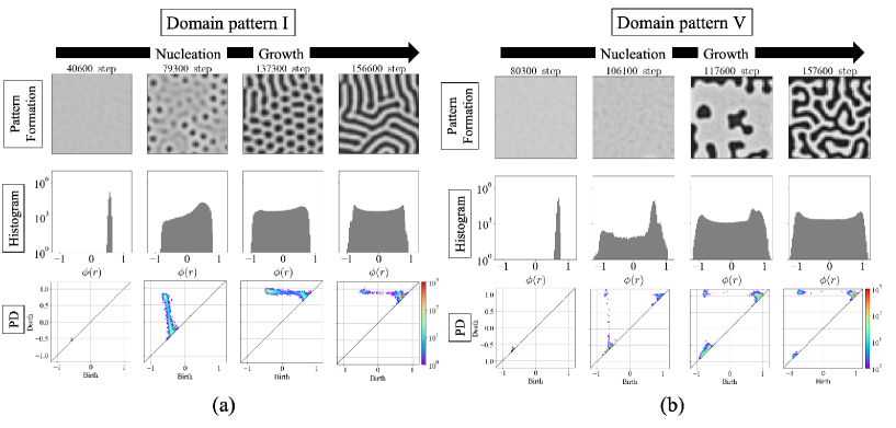
Figure 8: Process of magnetic domain pattern formation and the time evolution of the PD. The row showing pattern formation in the figure displays the time evolution of the magnetic domain pattern itself, whereas the row showing histograms displays the time evolution of the histograms of the intensity distribution of the magnetic moment $\phi\left(\bm{r}\right)$. The row showing PDs displays the time evolution of the PD. (a) Process of labyrinthine pattern formation and the time evolution of the PD in a region with a small $\alpha$ (I). (b) Process of labyrinthine pattern formation and the time evolution of the PD in a region with a large $\alpha$ (V).

In this section, we elucidate the physical mechanism underlying the novel physical findings discovered in the previous section by TDA of the magnetic domain formation process. We focused on the processes of pattern formation of pattern states I and V because they have the same labyrinthine pattern but are not adjacent to each other in the parameter space $\alpha$–$v$, which prominently represents the novel physical findings. Examples of the magnetic domain pattern formation belonging to pattern states I and V are shown in the first row of Fig. 8. We calculate the PDs of pattern states I and V at each time of the evolution process until the formation of the magnetic domain pattern and analyze the transition of its topological features. The transitions of PD according to the formation processes of pattern states I and V are distinctly different. In particular, the second and third columns of Figs. 8(a) and (b) show the time when the inverse magnetic domain is generated and the time when the inverse magnetic domain grows to form a labyrinthine structure, respectively. The time when the inverse domain is generated is the time when the initial microregions with a value of $\phi<0$ are generated, and the growth time of the inverse domain is the time when the area of the inverse magnetic domain grows (see “Histogram” in Fig. 8). The pattern states I and V, which form the same magnetic domain structure, are found to have very different PD transition processes in their inverse magnetic domain generation and growth processes [see the rows of PD in Figs. 8(a) and (b)]. In other words, the PDs of pattern state I during the generation and growth of inverse magnetic domains have a continuous and elongated distribution structure, whereas the PDs of pattern state V have three separated distributions corresponding to ${\rm PD}_{\rm long}$ and ${\rm PD}_{\rm short}$.

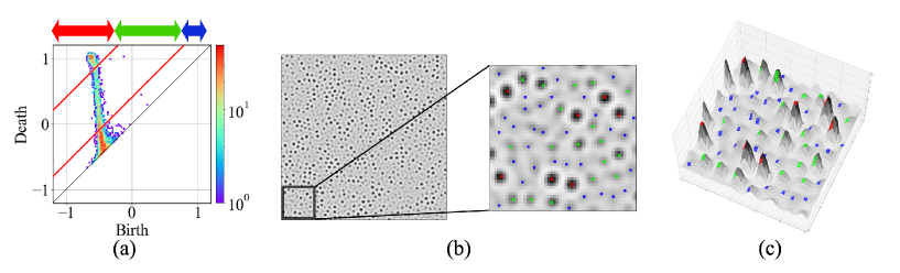
Figure 9: Correspondence between the distribution of generators and the magnetic domain pattern of the PD at the time of domain generation. (a) PD of the magnetic domain pattern ($\alpha=1.5$, $v=0.01$) around the time of domain generation, where the region with long-lifetime generators is indicated by a red arrow, the region with intermediate-lifetime generators is indicated by a green arrow, and the region with short-lifetime generators is indicated by a blue arrow. (b) Magnetic domain pattern and its magnified view. Each color point in the magnified image represents the position of each death cube corresponding to the lifetime region of the corresponding color in the PD. (c) Landscape of magnetic domain pattern, where each color point represents the position of each death cube corresponding to the lifetime region of the corresponding color in the PD. The HomCloud library[23] was used to extract the locations of death cubes.

The peculiar behavior of the PD at the time of generation of inverse magnetic domains is investigated by inverse analysis. The position of the death cube corresponding to the PD of pattern state I at the time of domain generation is given in Fig. 9. It is found that the continuous distribution structure of PD is due to the fact that the generated domains take not only large positive and small negative values of the magnetic moment but also intermediate values. This inverse analysis suggests that, in the parameter region where $\alpha$ is small, the magnetic domains are formed through the continuous increase in the intensity of magnetic moment $\phi\left(\bm{r}\right)$. On the other hand, in the region where $\alpha$ is large, the magnetic domains do not take the intermediate intensity of magnetic moments and they emerge discretely.

To investigate how the continuous and discrete magnetic domain generation processes are related to the dominant parameters $\alpha$ and $v$ of the system, we quantify the degree to which the inverse magnetic domains take intermediate states during their generation and growth as follows. First, we generated a histogram from the magnetic domain pattern data $\phi\left(\bm{r}\right)_{t=2T_{0}}$ at $t=2T_{0}$, and the values of the positive peaks $\phi_{\rm max}$ and negative peak $\phi_{\rm min}$ were obtained. Similarly, we obtained the standard deviations of the magnetic moment in the $\phi\left(\bm{r}\right)_{t=2T_{0}}\leq 0$ and $\phi\left(\bm{r}\right)_{t=2T_{0}}>0$ regions called $\sigma_{\rm+}$ and $\>\sigma_{\rm-}$, respectively. We define the condition under which the lifetime $\Delta t^{\prime}_{\rm mid\>life}$ of the hole corresponding to the domain in the intermediate state should be satisfied as

$$(\phi_{\rm min}+2\sigma_{\rm-})<\Delta t^{\prime}_{\rm mid\>life}<(\phi_{\rm max}-2\sigma_{\rm+}).$$ (29)

Note that the terms $t^{\prime}$ and lifetime do not correspond to the time of the pattern formation process, but to the threshold for binarizing a grayscale image to calculate PH. Moreover, the range of the birth time $t^{\prime}_{\rm birth}$ values of the generators involved in domain generation is defined as

$$t^{\prime}_{\rm birth}\leq\phi_{\rm min}+2\sigma_{\rm-},$$ (30)

and the range of the death time $t^{\prime}_{\rm death}$ values of the generators involved in domain growth is defined as

$$t^{\prime}_{\rm death}\geq\phi_{\rm max}-2\sigma_{\rm+}.$$ (31)

A hole that has a lifetime in the range of $\Delta t^{\prime}_{\rm mid\>life}$ and its birth is earlier than $t^{\prime}_{\rm birth}$ is defined as a generator in an intermediate state during domain generation. A hole that has a lifetime in the range of $\Delta t^{\prime}_{\rm mid\>life}$ and its death is later than $t^{\prime}_{\rm death}$ is defined as a generator in an intermediate state during domain growth. For example, from these definitions, the intermediate state of domain generation and domain growth corresponds to the red regions in Figs. 10(a) and (c). Let $N^{\rm gen}_{\rm mid}$ and $N^{\rm grow}_{\rm mid}$ be the numbers of generators within these intermediate states of domain generation and growth, respectively, and let $N_{\rm all}$ be the number of generators in the PD. Then, the ratios of the number of generators in the intermediate states during domain generation and growth to the total number of generators are defined respectively as follows:

$$R^{\rm gen}(t) := \frac{N^{\rm gen}_{\rm mid}(t)}{N_{\rm all}(t)}$$ (32)

$$R^{\rm grow}(t) := \frac{N^{\rm grow}_{\rm mid}(t)}{N_{\rm all}(t)}$$ (33)

As an indicator of whether or not intermediate states occur during the generation and growth, the maximum ratios of $R^{\rm gen}(t)$ and $R^{\rm grow}(t)$ are defined respectively as

$$R^{\rm gen}_{\rm max} := R(t^{\rm gen}_{\rm max}),\>\>\>\>\>t^{\rm gen}_{\rm max}:=\mathop{\rm arg~{}max}\limits_{t}R^{\rm gen}(t),$$ (34)

$$R^{\rm grow}_{\rm max} := R(t^{\rm grow}_{\rm max}),\>\>\>\>\>t^{\rm grow}_{\rm max}:=\mathop{\rm arg~{}max}\limits_{t}R^{\rm grow}(t).$$ (35)

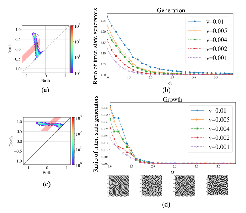
Figure 10: Relationship of the ratio of the number of generators in intermediate state with the total number of generators and $\alpha$ and $v$. (a) PD around the time of domain generation, where the red region is defined as the region of the intermediate state of domain generation. (b) Ratio of generator number with intermediate state around the time of domain generation. The horizontal axis is $\alpha$, and the vertical axis is the ratio of generator $R^{\rm gen}_{\rm max}$ with intermediate state. (c) PD around the time of domain growth, where the red region is defined as the region of the intermediate state of domain growth. (d) Ratio of generator number with intermediate state around the time of domain growth. The horizontal axis is $\alpha$, and the vertical axis is the ratio of generator $R^{\rm grow}_{\rm max}$ with intermediate state.

It is confirmed that $R^{\rm gen}$ and $R^{\rm grow}$ at $v<0.005$ take relatively large values when $\alpha<2.0$, and decrease rapidly to 0 at around $\alpha=2.0$ [Figs. 10(b) and (d)]. This result indicates that there are two types of magnetic domain pattern formation process for the same labyrinthine structure: one involves inverse magnetic domains that were generated and grew discontinuously, and the other involves those that were generated and grew continuously. The parameter regions of the first and second types of formation process correspond approximately to the parameter regions of pattern states I and V, respectively. In addition, $\alpha=2.0$, where this magnetic domain pattern formation process transitioned, corresponds to the region of pattern states III and IV, which are the sea-island structure and mixed states, respectively.

The result that different magnetic domain formation processes occur rapidly as $\alpha$ increases can be understood from $H_{\mathrm{ani}}$, whose relative intensity is controlled by $\alpha$. In other words, since $\alpha$ represents the intensity of magnetic anisotropy, it is easier to form an intermediate state when this value is small, and it is more difficult to form an intermediate state when this value is large. These insights are also obtained owing to the treatment of $\phi\left(\bm{r}\right)$ as a continuous value in TDA. We can quantitatively determine that there are two types of domain formation process in labyrinthine structures using methods other than PH-based feature extraction, such as analysis of histograms. However, in the first place, without confirmation of the clear difference between state transitions observed in the PH-based feature extraction (Fig. 8), it is difficult to see the difference. In the next section, this intuitive understanding will be discussed more elaborately by analyzing the energy function.

VI Discussion

In this section, by analyzing the energy function, we discuss why there are two types of magnetic domain pattern formation process for similar labyrinthine structures but have different domain formation processes, which change from continuous to discrete formation depending on the increase in $\alpha$.

From the results of numerical simulations, it can be seen that when an inverse magnetic domain is generated, the region other than the inverse magnetic domain does not change in response to changes in the external magnetic field, but only the region within the inverse magnetic domain changes (see Appendix D). Therefore, by placing the scalar variable $\phi$ as the magnetic moment characterizing the inverse magnetic domain, the energy function $H(\phi\left(\bm{r}\right))$ [Eq. (2)] is reduced to the following energy function $H^{\prime}(\phi)$ (see Appendix D):

$$H^{\prime}(\phi)=w_{0}(\beta)+w_{1}(\beta,\gamma,h(t))\phi+w_{2}(\alpha,\beta,\gamma)\phi^{2}+w_{4}(\alpha)\phi^{4},$$ (36)

where $w_{0}$, $w_{1}$, $w_{2}$, and $w_{4}$ represent constants independent of $\phi$. If we focus on the case where an isomorphic magnetic domain is generated, we find that $w_{1}\propto-h(t)+C_{1}(\alpha)\propto t-C^{\prime}_{1}(\alpha)$, $w_{2}\propto-\alpha+C_{2}$, $w_{4}\propto\alpha>0$, and $C_{2}>0$. Since only $w_{1}\phi$ is an asymmetric term of energy function $H^{\prime}(\phi)$, $w_{1}<0$ at $t=0$ and changes to $w_{1}>0$ around the time of domain generation. If $H^{\prime}(\phi)$ takes a sufficiently large $\alpha$ and the system exist around domain generation $w_{1}\sim 0$, then we find that $H^{\prime}(\phi)$ has two minimal solutions from the discriminant formula $D$ for the cubic equation $\frac{dH^{\prime}(\phi)}{d\phi}=0$. Similarly, the fact that $w_{1}\propto t$ and $w_{1}>0$ after the domain generation demonstrates that $w_{1}$ with a positive value increases with time and that there is a single minimal solution for the cubic equation $\frac{dH^{\prime}(\phi)}{d\phi}=0$. This indicates that for an energy function with two minimal solutions around the time of domain generation when the value of $\alpha$ is sufficiently large, one of the minimal solutions is eliminated with time. Since the TDGL equation is a deterministic time evolution model, the system is expected to remain in a metastable state until the minimal solution of the energy function is retained. This type of evolution of an energy landscape at a large $\alpha$ suggests that domain generation passes through supersaturation states ($\alpha>2.0$ in Fig. 11). Similarly, when the value of $\alpha$ is small and there is only one minimal solution even around the time of domain generation, the number of minimal solutions remains to be one despite the increase in time. This explains the occurrence of continuous domain generation seen when $\alpha<2.0$ (Fig. 11). This drastic change of the energy landscape with $\alpha$ is the mechanism behind the two similar pattern states I and V with different formation processes.

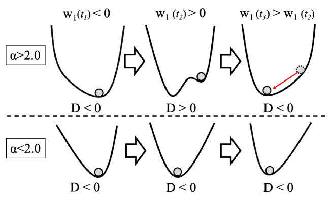
Figure 11: Schematic diagram of the generation mechanism of two different inverse magnetic domains such as pattern states I and V. The time evolution of the reduced energy landscape with the scalar variable $\phi$ is shown. $\phi$ is a representative value of the magnetic moment of the inverse domain.

From this reduced energy model, we can also discuss the mechanism of the sea-island state III and mixed states II and IV at around $\alpha=2.0$. $\alpha\sim 2.0$ should be the boundary parameter region between the continuous and discontinuous magnetic domain generation ($w_{2}\sim 0$). Therefore, owing to the spatial inhomogeneity $\lambda$ of anisotropy, some spatial regions are expected to be continuous and others discrete in magnetic domain generation. Compared with the case where magnetic domains are generated continuously, the discrete generation of magnetic domains is relatively delayed because the magnetic domains are not generated until the bimodal structure is resolved. A state in which there is already an inverse magnetic domain can be seen as an additional negative external magnetic field. This might prevent the resolution of the bimodal structure, thus creating a structure that partially lacks the labyrinthine structure. Although we only discussed the domain generation here, similar mechanisms are expected to work in domain growth. Thus, we can confirm that PH is capable of extracting useful features that can provide novel mechanisms of the magnetic domain pattern formation process.

VII Summary

In this study, by treating $\phi\left(\bm{r}\right)$ as a continuous value using PH, we obtained the following findings that have not been obtained in previous studies of magnetic domain formation using the TDGL equation.

1. The intensity fluctuations in the domain are strongly correlated with the properties $\alpha$ and $v$.

2. As $\alpha$ continuously changes, the magnetic domain pattern changes from a labyrinthine structure to an sea-island structure or a mixture of the two, and then back to a labyrinthine structure.

3. There are two types of magnetic domain pattern formation process for similar labyrinthine structures: discontinuous inverse magnetic domain formation and continuous inverse magnetic domain formation.

4. The cause of the qualitative transition in pattern formation dynamics depending on the value of $\alpha$ might be the occurrence of a transition of the energy landscape.

These findings also suggest the importance of measuring landscape structures of magnetic domain accurately to experimental researchers.

PH-based features should be useful not only for the TDGL equation, but also for the analysis of systems in the continuum approximation with similar energy functions and the corresponding measurement data. Furthermore, because PD can estimate physical properties and analyze time-series data, it is possible to develop a prediction model of the time evolution of physical properties using the time evolution model of the PD. The analysis procedure with PH presented in this paper gives one format applicable to extracting scientific knowledge from a wide range of pattern formation processes with long-range interactions.

Appendix A Differences in PH groups due to differences in construction method of cubical complex

The term “holes” has been used ambiguously in the main text. Depending on how holes are quantified from the figure data, different PH groups are obtained from the same data. This section explains how construction method of cubical complex produce different PH groups. For this purpose, the calculation procedure for PD is explained in detail. The characteristics of each PH group obtained by the two libraries with different construction methods employed in this study, GUDHI[29] and HomCloud[23] library, are described in the last paragraph of this appendix.

To establish holes quantitatively, figure data are first reexpressed as a set of triangles (a simplicical complex) or rectangles (a cubical complex) to ensure that they can be dealt with algebraically. When grayscale pixel image data $G:=\{G(i,j)\in[0,1]\mid\>1\leq i\leq d_{x},1\leq j\leq d_{y}\}$ are provided as input data, they are converted to a cubical complex using the following data structure: we consider the grayscale pixel data as a set of binary images binarized at a certain threshold $t$ which is expressed as

$$G = \{G^{\rm binary}_{t}\mid t\in[t_{\rm min},t_{\rm max}]\},$$ (37)

$$G^{\rm binary}_{t} = \{G(i,j)\mid G(i,j)\geq t\},$$ (38)

and represent each binary image $G^{\rm binary}_{t}$ as a cubical complex $K^{t}$. A pixel in a binary image $G^{\rm binary}_{t}$ is considered a rectangle, and the structure of this image can be covered by rectangles [Fig. 1(b), upper panel]. Because a rectangle is a closed convex set, this coverage can be considered a representation of a figure by a set of closed convex sets. A set of closed convex sets can be transformed into a cubical complex with the same topological structure. For example, by mapping a convex set (pixel) to a cube, a cubical complex can be constructed as follows [Fig. 1(c), upper panel]: If a pixel $G(i,j)$ belongs to a domain, then a zero-dimensional cube denoted as $[i,i]\times[j,j]$, called a zero-cube or point, is placed at the center of a rectangle. If a neighboring pixel $G(i,j)$ of $G(i\pm 1,j)$ or $G(i,j\pm 1)$ belongs to a domain, then we assume that $G(i,j)$ and neighboring pixels are connected, and set a one-dimensional cube, called a one-cube or line, which is represented as $[i,i\pm 1]\times[j,j]$ or $[i,i]\times[j,j\pm 1]$. Similarly, if four adjacent pixels $G(i,j)$, $G(i+\delta_{i},j)$, $G(i,j+\delta_{j})$, and $G(i+\delta_{i},j+\delta_{j})$, where $\delta_{i}=\pm 1$ and $\delta_{j}=\pm 1$ belong to a domain, we set a two-dimensional cube, called a two-cube or square, which is denoted as $[i,i+\delta_{i}]\times[j,j+\delta_{j}]$. For pixel data with $d$ dimensions ($d\geq 3$), we can also set a higher-order cube $[i_{1},i_{1}+\delta_{i_{1}}]\times[i_{2},i_{2}+\delta_{i_{2}}]\times\cdots\times[i_{d},i_{d}+\delta_{i_{d}}]$. By appropriately combining the above-mentioned squares, $G^{\rm binary}_{t}$ is represented as a set of cubes or cubical complexes $K_{t}$. The cube elements of $K_{t}$ increase as the threshold, $t$, decrease. Here, the threshold value $t$ is replaced by $t^{\prime}=1-t$ to let the increase of threshold value correspond to the increasing sequence of cube elements. the sequence of cube elements of $K_{t^{\prime}}$ which is created according to an increase of threshold $t^{\prime}$ forms a monotonically increasing sequence. Such an increasing sequence is called a filtration $\mathbf{K}$.

$$\mathbf{K}:=K_{t_{1}}\subset K_{t_{2}}\cdots\subset K_{t_{n_{\Theta}}}$$ (39)

where $0\leq t^{\prime}_{k}<t^{\prime}_{k+1}\leq 1$ and $n_{\Theta}$ is the total number of thresholds $t^{\prime}$ at which a cube belonging to $\mathbf{K}$ is generated depending on the increase in $t^{\prime}$. To capture the change in a graphic structure due to threshold $t^{\prime}$, we consider the following vector in an $n_{\Theta}$-dimensional space:

$$\hat{\sigma}_{m}=(0,0,\ldots,0,\sigma_{m},0,\ldots,0),$$ (40)

where the non-zero element $\sigma_{m}$ is located at the $n_{b_{m}}$-th element of the vector, and the $n_{b_{m}}$-th element corresponds to threshold $b_{m}$ at which a certain cube $\sigma_{m}$ generated. Consider an operator $x$ that acts on this vector space and shifts one element to the right (i.e., moves to the threshold where the next young cube is generated) as follows:

$$x(c_{1},c_{2}\cdots)=(0,c_{1},c_{2},\ldots)$$ (41)

Thus, all cube elements in each cubical complex corresponding to $\mathbf{K}$, which vary with threshold $t^{\prime}$, can be represented using the basis vector in Eq. (40) and manipulate using the operator $x$. This representation allows us the algebraic manipulation of geometric elements of the figure, such as cubical complexes.

Geometrical structures, such as cycles and boundaries, can also be defined and manipulated algebraically by representing them in the same manner. Here, we simplify a figure as a binary image and explain the concepts of a cycle, boundary, and hole by assuming that the vector of the cubical complex is one dimensional, i.e., $\hat{\sigma}_{m}=\sigma_{m}$. It corresponds to the definition of a cycles and boundaries for a binary image in the homology group.

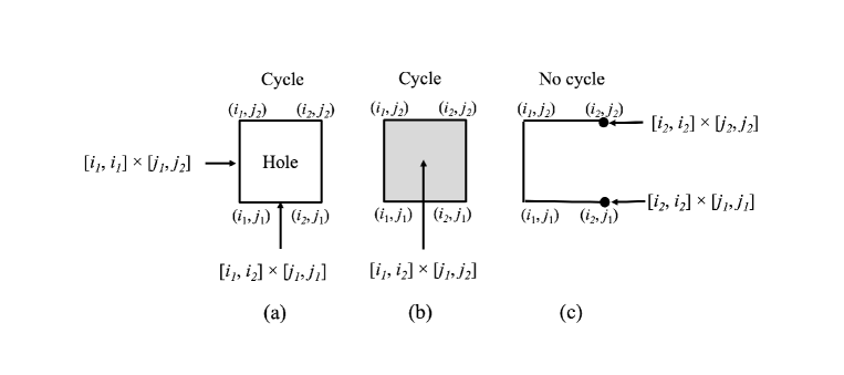
Figure 12: Examples of cubical complexes with (a) a cycle and hole, and (b) a cycle filled by a two-cube, and (c) a one-cubical complex with a two-boundary structure. The boundaries comprise the endpoints of the cubical complex.

A $d$-dimensional cycle, which is the candidate of a hole, is a $d$-dimensional cubical complex with a boundary less structure [Figs. 12(a) and (b)]. The boundary of a cubical complex comprises its endpoints. For example, if a cubical complex is a line (one-cube) $[i_{1},j_{1}]\times[i_{2},i_{2}]$ where $i_{1}\neq j_{1}$, then both endpoints (zero-cubes) of the line, $[i_{1},i_{1}]\times[i_{2},i_{2}]$ and $\>[j_{1},j_{1}]\times[i_{2},i_{2}]$, form its boundary. If a cubical complex is a rectangle (two-cube) $[i_{1},j_{1}]\times[i_{2},j_{2}]$ where $i_{1}\neq j_{1}$ and $i_{2}\neq j_{2}$, then its boundary comprises four lines (one-cubes) around a two-cube: $[i_{1},j_{1}]\times[i_{2},i_{2}],\>[i_{1},j_{1}]\times[j_{2},j_{2}],\>[i_{1},i_{1}]\times[i_{2},j_{2}]$, and $[j_{1},j_{1}]\times[i_{2},j_{2}]$. Thus, a boundaryless connection signifies that the endpoints of each cube are connected without excess or deficiency, such as $[i_{1},j_{1}]\times[i_{2},i_{2}],\>[i_{1},j_{1}]\times[j_{2},j_{2}],\>[i_{1},i_{1}]\times[i_{2},j_{2}]$, and $[j_{1},j_{1}]\times[i_{2},j_{2}]$. Specifically, to be a cycle, there should be exactly two multiples of the endpoint structures of the shape when adding the endpoint structures of each side. This is expressed as follows:

$$([i_{1},i_{1}]\times[i_{2},i_{2}]+[j_{1},j_{1}]\times[i_{2},i_{2}])+([j_{1},j_{1}]\times[i_{2},i_{2}]+[j_{1},j_{1}]\times[j_{2},j_{2}])$$ (42)

$$+ ([j_{1},j_{1}]\times[j_{2},j_{2}]+[i_{1},i_{1}]\times[j_{2},j_{2}])+([i_{1},i_{1}]\times[j_{2},j_{2}]+[i_{1},i_{1}]\times[i_{2},i_{2}])$$

$$= 2([i_{1},i_{1}]\times[i_{2},i_{2}])+2([j_{1},j_{1}]\times[i_{2},i_{2}])+2([j_{1},j_{1}]\times[j_{2},j_{2}])+2([i_{1},i_{1}]\times[j_{2},j_{2}]).$$

Thus, the condition for a given cubical complex to constitute a cycle is that the coefficients resulting from the addition of the boundary structures are multiples of 2. To provide a more explicit indicator of the presence or absence of such a cycle, we replace the coefficient from adding the cube complexes corresponding to the endpoints with the remainder of dividing that coefficient by 2, i.e., the coefficient is replaced from integer $\mathbf{Z}$ to factor ring $\mathbf{Z_{2}}$. Consequently, the addition of zero-cubes corresponding to endpoints of one-cubes is expressed as follows:

$$2([i_{1},i_{1}]\times[i_{2},i_{2}])+2([j_{1},j_{1}]\times[i_{2},i_{2}])+2([j_{1},j_{1}]\times[j_{2},j_{2}])+2([i_{1},i_{1}]\times[j_{2},j_{2}])$$ (43)

$$= 0([i_{1},i_{1}]\times[i_{2},i_{2}])+0([j_{1},j_{1}]\times[i_{2},i_{2}])+0([j_{1},j_{1}]\times[j_{2},j_{2}])+0([i_{1},i_{1}]\times[j_{2},j_{2}])$$

$$= 0.$$

Thus, finding a cycle corresponds to finding structures in which the boundaries of a cubical complex are added and their coefficients are zero. A d-dimensional hole is defined as a $d$-dimensional cycle that is not filled by a (d+1)-dimensional cubical complex, i.e., a $d$-dimensional cycle that is not the boundary of a (d+1)-dimensional cubical complex [Fig. 12(a)]. Therefore, to extract the subset of a cubical complex corresponding to a hole, we take the difference (quotient set) between the subset of a $d$-dimensional cubical complex representing d-dimensional cycle structures and the set of a $d$-dimensional cubical complex that forms the boundary of a ($d+1$)-dimensional cubical complex.

For a grayscale image, if the threshold $t^{\prime}$ at which a boundary is generated or disappears is known, the threshold at which hole $k$ is generated $b_{k}$ and disappears $d_{k}$ can be calculated. The PD can be calculated if the pairs of $b_{k}$ and $d_{k}$ for all holes are obtained. For this purpose, a boundary is treated in the vector space in the same way as $\hat{\sigma}_{m}$. The boundary $\hat{\sigma}^{l}_{m}$, which is the boundary of an $l$-dimensional cube generated at $m$, is obtained as

$$\partial_{l}\left(\hat{\sigma}^{l}_{m}\right) = \partial_{l}\left(0,0,\ldots,[i_{1},j_{1}]\times[i_{2},j_{2}]\times\cdots\times[i_{l},j_{l}],\ldots,0,0\right)$$

$$:= \sum_{k=1}^{l}\left[x^{b(\sigma^{l}_{m})-b(\sigma^{l-1}_{i_{k}})}\left(0,0,\ldots,\sigma^{l-1}_{i_{k}},\ldots,0,0\right)\right.$$

$$+ x^{b(\sigma^{l}_{m})-b(\sigma^{l-1}_{j_{k}})}\left.\left(0,0,\ldots,\sigma^{l-1}_{j_{k}},\ldots,0,0\right)\right],$$ (45)

$$\sigma^{l-1}_{i_{k}} := [i_{1},j_{1}]\times\cdots\times[i_{k},i_{k}]\times\cdots\times[i_{l},j_{l}],$$ (46)

$$\sigma^{l-1}_{j_{k}} := [i_{1},j_{1}]\times\cdots\times[j_{k},j_{k}]\times\cdots\times[i_{l},j_{l}],$$ (47)

where $\partial_{l}\left(\hat{\sigma}^{l}\right)$ is a vector whose elements correspond to the threshold at which the boundary is generated, $i_{s}\neq j_{s}$ for all $s$, and $b(\cdot)$ represents the index of vector $\hat{\sigma}_{m}$ [Eq. (40)], and corresponds to the threshold at which the $l$-dimensional cube, $\sigma_{m}$, generates. $\partial_{l}\left(\hat{\sigma}^{l}\right)$ is called a boundary operator. In the case of a binary image, the boundary set of cubical complex that add to zero correspond to a cycle. When adding the vector elements in $\partial_{l}\left(\hat{\sigma}^{l}\right)$, each vector element is multiplied by the exponentiation of $x$ to align the vector elements. Thus, in the case of a grayscale image, a cycle that is not a boundary is calculated as the case of the binary image. Accordingly, the persistence interval $I$ and persistent diagram $PD(\mathbf{K})$ specifying the PH group is calculated algebraically in the vector space. Thus, once pixel image data are covered by convex sets, the PH group can be calculated.

Here, we explain the changes in the calculated PH groups due to the difference in the methods used to cover pixel image data by convex sets. One approach to covering pixel image data $G_{t^{\prime}}(i,j)$, which are binarized at a certain threshold $t^{\prime}$, is to cover one pixel as a single cube, as described above. This coverage treats adjacent diagonal pixels as if they are disconnected. Another type of relationship can be considered as a connected cubical complex by setting zero-cubes (points) at the center of a pixel, its four corners, and its four border lines [Fig. 1(b), upper panel]. In this study, the latter type of coverage was chosen because it can extract more diverse information about an object. The calculation of PH groups based on such coverage was implemented in the GUDHI library[29]. In this study, the HomCloud library[23] was also used to extract the pixels corresponding to the center of a death cube to understand the PDs. The HomCloud library uses a coverage method that sets a single zero-cube at the center of a pixel. Therefore, it should be noted that in the analysis of the location of a death cube, as described in Sec. IV.1, not all rectangle locations obtained in the GUDHI library were extracted; instead, only their approximate properties were derived.

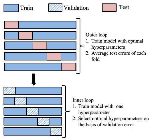
Figure 13: Procedure for the nested cross-validation method[24].

Appendix B Procedure for the nested cross-validation method

Nested cross-validation estimates the generalization error of the underlying model and its hyperparameters based on two cross-validations in a nested relationship (i.e., an inner loop and an outer loop). The detailed procedures for both loops are described in Fig. 13. In the innerloop, the model is trained with one hyperparameter, and the optimal hyperparameters are selected based on the validation error. In the outerloop, the model is trained with optimal hyperparameters obtained from the innerloop, and the prediction error of the model is the average of the test errors of each fold.

Appendix C Additional analyses for magnetic-domain patterns at $t=2T_{0}$

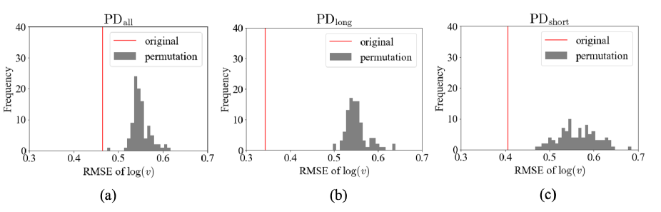
Figure 14: Results of the permutation test for (a) ${\rm PD}_{\rm all}$, (b) ${\rm PD}_{\rm long}$, and (c) ${\rm PD}_{\rm short}$.

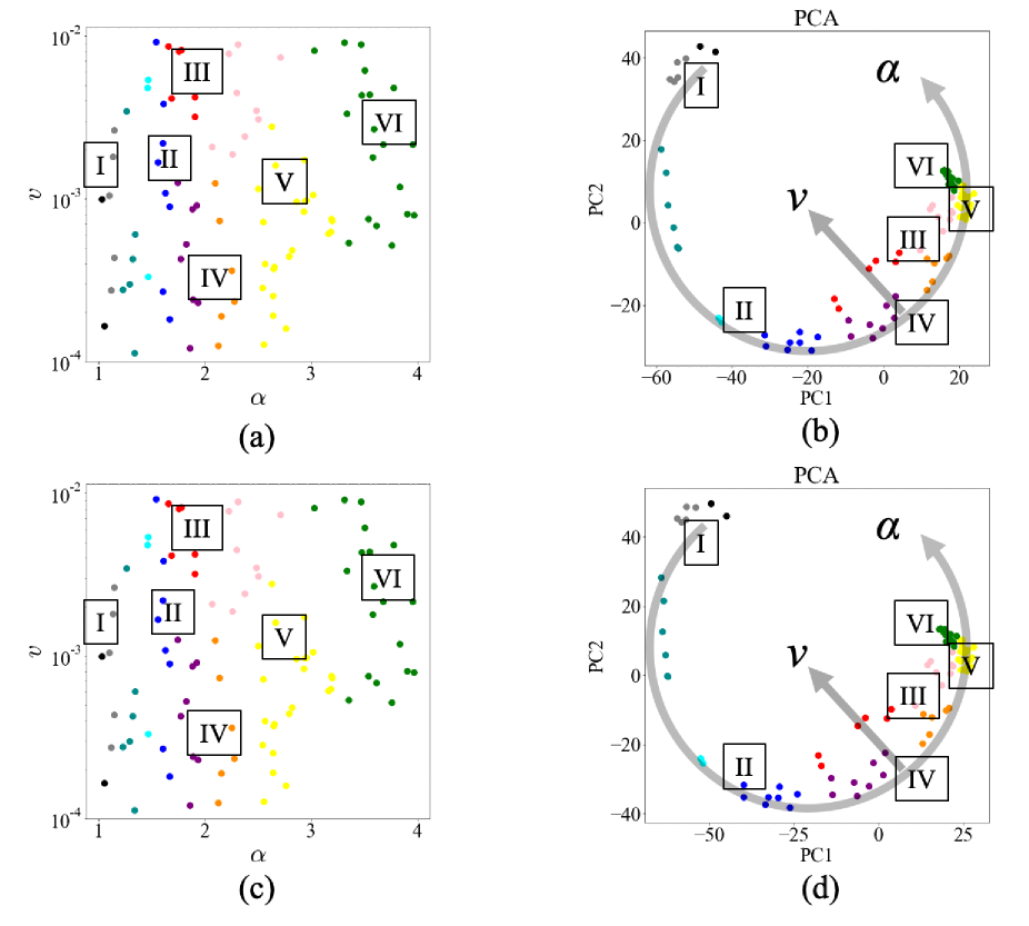
Figure 15: Clustering results of the K-means method and results of the PCA. (a) K-means clustering results of the PDs vectorized with parameters $\sigma$ and $d$ estimated by regression analysis of $\alpha$. (b) Results of the PCA of the PDs vectorized with parameters $\sigma$ and $d$ estimated by regression analysis of $\alpha$. (c) K-means clustering results of the PDs vectorized with parameters $\sigma$ and $d$ estimated by a regression analysis of $\log\>\>v$. (d) Results of a PCA of the PDs vectorized with parameters $\sigma$ and $d$ estimated by a regression analysis of $\log\>\>v$.

Three additional analyses were conducted to support the conclusions drawn from the analysis of a magnetic domain pattern at $t=2T_{0}$ discussed in the main text. The first was a statistical validation that suggests that the PDs are a good feature for estimating $\log\>v$. Under the ridge regression of $\log\>v$ with nested cross-validation that is described in the previous section (Appendix B), we statistically tested whether the PDs contain the information required to estimate $\log\>v$. In the verification, the RMSE distribution by permutation of the objective variable of the regression, $\log\>\>v$, was calculated and used to the statistical test whether the regression accuracy of the original data was significantly high. The results of this permutation test confirmed that for all ${\rm PD}$, the estimation accuracy of $\log\>v$ of the original data was significantly higher than that of the permutated data (Fig. 14). These results suggest that the vectorized data of the three parts of the ${\rm PD}$ are good features for estimating $\log\>v$.

The second additional analysis supported the K-means clustering results based on ${\rm PD}_{\rm all}$. The clustering results using vectorization parameters $\sigma$ and $d$ of the PDs obtained from the regression analysis of $\log\>v$ were not included in the analysis presented in the main text. Therefore, in this section, we show these results in Fig. 15. The exact same clustering results and the similar PCA results in the case of $\alpha$ were obtained.

In the last analysis, K-means clustering results were compared with results determined by other clustering methods. As shown in Fig. 16, the clustering results are similar to the K-means method results under appropriate parameter settings, which demonstrates the robustness of the clusters obtained by the K-means method.

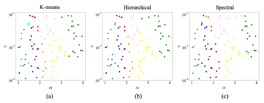
Figure 16: Clustering results from various clustering methods. (a) Clustering results using the K-means method. The number of clusters is determined using the elbow method[28] (see main text). (b) Clustering results using the hierarchical clustering method[30]. The hierarchy clustering method is adopted with the following hyperparameters: metric = euclidean, Linkage criteria = ward, and number of clusters K = 11. (c) Clustering results using the spectral clustering method[31]. The spectral clustering library is adopted with the following hyperparameters: affinity matrix = polynomial function with degree = 5, and kernel coefficient for polynomial function = 0.0001. The number of clusters is optimized using the elbow method and determined as K = 9.

Appendix D Analysis of the energy landscape in inverse magnetic domain generation

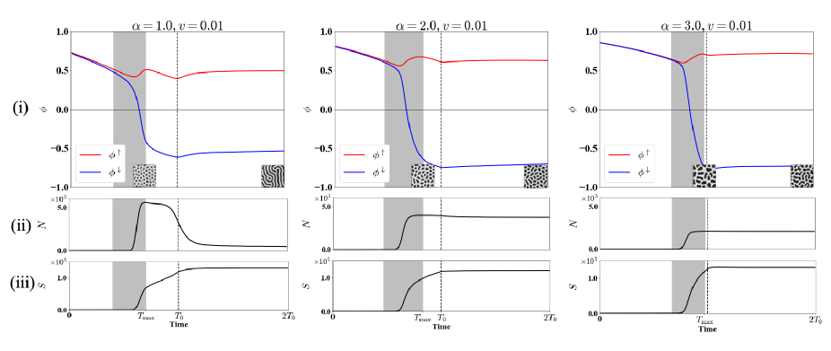
Figure 17: Time evolution of the average magnetic moment during domain generation at $v=0.01$ and $\alpha=1.0$, $2.0$, and $3.0$. The time region of the domain generation is shown in gray. The time at which the total number of domains $N$ is the largest is set to be the completion time of the domain generation $T_{\rm max}$, and the first time at which $N$ is greater than zero is set to be the start time of generation. (i) Time evolution of the average magnetic moment $\phi^{\downarrow}$ in the region in which the magnetic moment becomes negative in column $T_{\rm max}$ and is maintained until $2T_{0}$ together with the time evolution of the average magnetic moment $\phi^{\uparrow}$ in the region in which it is positive. (ii) Column time evolution of the total number of domains $N$. (iii) Column time evolution of the area of the inverse magnetic domain region ($\phi<0$).

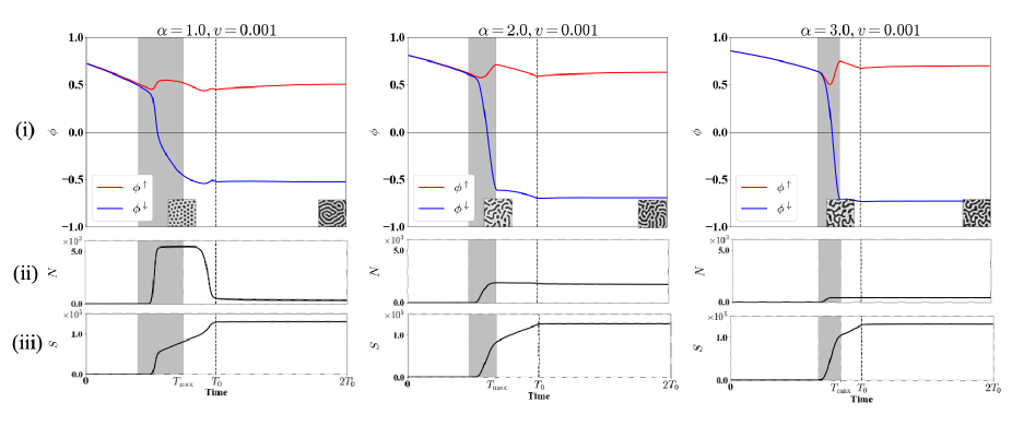
Figure 18: Time evolution of the average magnetic moment during domain generation at $v=0.001$ and $\alpha=1.0$, $2.0$, and $3.0$. The time region of the domain generation is shown in gray. The time at which the total number of domains $N$ is the largest is set to be the completion time of the domain generation $T_{\rm max}$, and the first time at which $N$ is greater than zero is set to be the start time of generation. (i) Time evolution of the average magnetic moment $\phi^{\downarrow}$ in the region in which the magnetic moment becomes negative in column $T_{\rm max}$ and is maintained until $2T_{0}$ together with the time evolution of the average magnetic moment $\phi^{\uparrow}$ in the region in which it is positive. (ii) Column time evolution of the total number of domains $N$. (iii) Column time evolution of the area of the inverse magnetic domain region ($\phi<0$).

In this appendix, by focusing on the structural change in the energy landscape, we analytically reveal the mechanism of the qualitative transition of the inverse magnetic domain generation process due to the increase in $\alpha$ as described in Sec. V. We define $T_{\rm max}$ as the time at which the number of isolated domains in the inverse magnetic domain reaches a maximum, and use it as the approximate end time of the inverse magnetic domain generation. The region that becomes an inverse magnetic domain at $T_{\rm max}$ and is maintained until $2T_{0}$ is denoted as $D_{T_{\rm max}}^{\downarrow}$, and the region that does not is denoted as $D_{T_{\rm max}}^{\uparrow}$. In the time domain in which the inverse magnetic domain occurs, the magnetic moment of $D_{T_{\rm max}}^{\downarrow}$ changes significantly, whereas that of $D_{T_{\rm max}}^{\uparrow}$ does not [Figs. 17(i) and 18(i)]. Using this knowledge, the magnetic moment $\phi(\bm{r})$ at the time of domain generation can be simplified using representative values of a scalar variable $\phi$ as

$$\phi(\bm{r})=\begin{cases}\phi\>\>\>(\bm{r}\in D_{T_{\rm max}}^{\downarrow})&\\ C(\alpha)\>\>\>(\bm{r}\in D_{T_{\rm max}}^{\uparrow})&\end{cases},$$ (48)

where $C={\rm const}$.

By substituting this simplified model into the energy function in Eq. (2), we derive the coarse-grained energy function $H(\phi)$, expressed in terms of the representative values of the magnetic moments of the inverse magnetic domain, $\phi$. If the area of the inverse magnetic domain region at $T_{\rm max}$ is $S_{\rm max}$, the boundary length of the inverse magnetic domain region is $L_{\rm max}$, area of $D_{\downarrow}$ is $S$, and the boundary length is $L$. Thus, the energy function in Eq. (2) at the time of inverse magnetic domain generation is

$$H(\phi(\bm{r})) = H^{\prime}(\phi)=H_{\rm ani}^{\prime}(\phi)+H_{\rm J}^{\prime}(\phi)+H_{\rm di}^{\prime}(\phi)+H_{\rm ex}^{\prime}(\phi)$$

$$= \alpha S\lambda\left(-\frac{\phi^{2}}{2}+\frac{\phi^{4}}{4}\right)$$

$$+\beta\frac{L(C(\alpha)-\phi)^{2}}{2}$$

$$+\gamma\left[\int_{\bm{r}\in D_{T_{\rm max}}^{\downarrow}}d\bm{r}\int_{\bm{r}^{\prime}\in D_{T_{\rm max}}^{\uparrow}}d\bm{r}^{\prime}\frac{C(\alpha)\phi}{\left|\bm{r}-\bm{r}^{\prime}\right|^{3}}+\int_{\bm{r}\in D_{T_{\rm max}}^{\downarrow}}d\bm{r}\int_{\bm{r}^{\prime}\in D_{T_{\rm max}}^{\downarrow}}d\bm{r}^{\prime}\frac{\phi^{2}}{\left|\bm{r}-\bm{r}^{\prime}\right|^{3}}\right]$$

$$-h(t)S\phi+{\rm const.},$$ (50)

$$= w_{0}(\beta)+w_{1}(\beta,\gamma,h(t))\phi+w_{2}(\alpha,\beta,\gamma)\phi^{2}+w_{4}(\alpha)\phi^{4},$$ (51)

where $w_{0}$, $w_{1}$, $w_{2}$, and $w_{4}$ represent constants independent of $\phi$. If we consider only the case in which an isomorphic magnetic domain generates, we find that $w_{1}\propto-h(t)+C_{1}(\alpha)\propto t-C^{\prime}_{1}(\alpha)$, $w_{2}\propto-\alpha+C_{2}$, $w_{4}\propto\alpha>0$, and $C_{2}>0$. Because only $w_{1}\phi$ is an asymmetric term, $w_{1}<0$ at $t=0$ changes to $w_{1}>0$ around the domain generation.

$H^{\prime}(\phi)$ has two minimal solutions when the discriminant formula of $\frac{dH^{\prime}(\phi)}{d\phi}=0$,

$$D=-\left(\frac{w_{2}(\alpha,\beta,\gamma)}{2w_{4}(\alpha)}\right)^{3}-27\left(\frac{w_{1}(\alpha,\beta,\gamma)}{4w_{4}(\alpha)}\right)^{2},$$ (52)

is positive, and one minimal solution when it is negative. Since $\frac{w_{2}}{w_{4}}\propto\frac{-\alpha+C_{2}}{\alpha}=-1+\frac{C_{2}}{\alpha}$ decreases as $\alpha$ increases, the discriminant expression, $D$, increases. In particular, if $\alpha$ is sufficiently large and the system exist around domain generation $w_{1}\sim 0$, then $w_{2}$ is a large negative value and $D>0$. This demonstrates that in a large region of $\alpha$, $H^{\prime}(\phi)$ has two minimal solutions around time of domain generation. Similarly, the fact that $w_{1}\propto t$ and $w_{1}>0$ after the domain generation suggests that the absolute value of $w_{1}$ increases with time, and the discriminant expression, $D$, decreases. This demonstrates that for an energy function with two minimal solutions around time of domain generation when the value of $\alpha$ is sufficiently large, one of the minimal states can be eliminated as time evolves. This change in the energy landscape explains the nucleation-like inversion of the magnetic domain at $\alpha>2.0$, because in the deterministic time-evolution model of the TDGL equation, the metastable state remains stable until it is resolved (Fig. 11). Similarly, if the value of $\alpha$ is small and only one minimal solution exists even around the time of domain generation, the number of minimal solutions does not change with time. This explains the continuous domain generation at $\alpha<2.0$ (Fig. 11).

References

- Jagla [2004] E. A. Jagla, Numerical simulations of two-dimensional magnetic domain patterns, Physical Review E 70, 046204 (2004).
- Kudo et al. [2007] K. Kudo, M. Mino, and K. Nakamura, Magnetic domain patterns depending on the sweeping rate of magnetic fields, Journal of the Physical Society of Japan 76, 013002 (2007).
- Chen [2002] L.-Q. Chen, Phase-field models for microstructure evolution, Annual Review of Materials Research 32, 113 (2002).
- Gray and Scott [1983] P. Gray and S. Scott, Autocatalytic reactions in the isothermal, continuous stirred tank reactor: isolas and other forms of multistability, Chemical Engineering Science 38, 29 (1983).
- Kudo and Nakamura [2007] K. Kudo and K. Nakamura, Field sweep-rate dependence of magnetic domain patterns: Numerical simulations for a simple ising-like model, Physical Review B 76, 054111 (2007).
- Guiu-Souto et al. [2012] J. Guiu-Souto, J. Carballido-Landeira, and A. P. Munuzuri, Characterizing topological transitions in a turing-pattern-forming reaction-diffusion system, Physical Review E 85, 056205 (2012).
- Nahas et al. [2020] Y. Nahas, S. Prokhorenko, Q. Zhang, V. Govinden, N. Valanoor, and L. Bellaiche, Topology and control of self-assembled domain patterns in low-dimensional ferroelectrics, Nature communications 11, 1 (2020).
- König et al. [2004] P.-M. König, R. Roth, and K. Mecke, Morphological thermodynamics of fluids: shape dependence of free energies, Phys. Rev. Lett. 93, 160601 (2004).
- Mecke [1996] K. Mecke, Morphological characterization of patterns in reaction-diffusion systems, Physical Review E 53, 4794 (1996).
- Carlsson [2009] G. Carlsson, Topology and data, Bulletin of the American Mathematical Society 46, 255 (2009).
- Edelsbrunner [2014] H. Edelsbrunner, A short course in computational geometry and topology, Mathematical methods (Springer, 2014).
- Dłotko and Wanner [2016] P. Dłotko and T. Wanner, Topological microstructure analysis using persistence landscapes, Physica D: Nonlinear Phenomena 334, 60 (2016).
- Calcina and Gameiro [2021] S. S. Calcina and M. Gameiro, Parameter estimation in systems exhibiting spatially complex solutions via persistent homology and machine learning, Mathematics and Computers in Simulation 185, 719 (2021).
- Obayashi et al. [2018] I. Obayashi, Y. Hiraoka, and M. Kimura, Persistence diagrams with linear machine learning models, Journal of Applied and Computational Topology 1, 421 (2018).
- Vandaele et al. [2020] R. Vandaele, G. A. Nervo, and O. Gevaert, Topological image modification for object detection and topological image processing of skin lesions, Scientific Reports 10, 1 (2020).
- Dey et al. [2011] T. K. Dey, A. N. Hirani, and B. Krishnamoorthy, Optimal homologous cycles, total unimodularity, and linear programming, SIAM Journal on Computing 40, 1026 (2011).
- Gameiro et al. [2016] M. Gameiro, Y. Hiraoka, and I. Obayashi, Continuation of point clouds via persistence diagrams, Physica D: Nonlinear Phenomena 334, 118 (2016).
- Cohen-Steiner et al. [2007] D. Cohen-Steiner, H. Edelsbrunner, and J. Harer, Stability of persistence diagrams, Discrete Comput. Geom. 37, 103 (2007).
- Hubert and Schäfer [2008] A. Hubert and R. Schäfer, Magnetic domains: the analysis of magnetic microstructures (Springer Science & Business Media, 2008).
- Hauser et al. [2016] C. Hauser, T. Richter, N. Homonnay, C. Eisenschmidt, M. Qaid, H. Deniz, D. Hesse, M. Sawicki, S. G. Ebbinghaus, and G. Schmidt, Yttrium iron garnet thin films with very low damping obtained by recrystallization of amorphous material, Scientific reports 6, 1 (2016).
- Zomorodian and Carlsson [2005] A. Zomorodian and G. Carlsson, Computing persistent homology, Discrete & Computational Geometry 33, 249 (2005).
- Adams et al. [2017] H. Adams, T. Emerson, M. Kirby, R. Neville, C. Peterson, P. Shipman, S. Chepushtanova, E. Hanson, F. Motta, and L. Ziegelmeier, Persistence images: A stable vector representation of persistent homology, Journal of Machine Learning Research 18 (2017).
- [23] HomCloud, https://homcloud.dev/index.html.
- Cawley and Talbot [2010] G. C. Cawley and N. L. Talbot, On over-fitting in model selection and subsequent selection bias in performance evaluation, The Journal of Machine Learning Research 11, 2079 (2010).
- Rokach and Maimon [2005] L. Rokach and O. Maimon, Clustering methods, in Data mining and knowledge discovery handbook (Springer, 2005) pp. 321–352.
- Forgy [1965] E. W. Forgy, Cluster analysis of multivariate data: efficiency versus interpretability of classifications, biometrics 21, 768 (1965).
- MacQueen et al. [1967] J. MacQueen et al., Some methods for classification and analysis of multivariate observations, in Proceedings of the fifth Berkeley symposium on mathematical statistics and probability, Vol. 1 (Oakland, CA, USA, 1967) pp. 281–297.
- Thorndike [1953] R. L. Thorndike, Who belongs in the family?, Psychometrika 18, 267 (1953).
- Dłotko [2018] P. Dłotko, Computational and applied topology, tutorial, arXiv preprint arXiv:1807.08607 (2018).
- Maimon and Rokach [2005] O. Maimon and L. Rokach, Data mining and knowledge discovery handbook, (2005).
- Von Luxburg [2007] U. Von Luxburg, A tutorial on spectral clustering, Statistics and computing 17, 395 (2007).
- Seul et al. [1992] M. Seul, L. Monar, and L. O’Gorman, Pattern analysis of magnetic stripe domains morphology and topological defects in the disordered state, Philosophical Magazine B 66, 471 (1992).
- Abu-Libdeh and Venus [2011] N. Abu-Libdeh and D. Venus, Dynamics of topological defects in a two-dimensional magnetic domain stripe pattern, Physical Review B 84, 094428 (2011).
- Tibshirani [1996] R. Tibshirani, Regression shrinkage and selection via the lasso, Journal of the Royal Statistical Society: Series B (Methodological) 58, 267 (1996).
- Baum and Petrie [1966] L. E. Baum and T. Petrie, Statistical inference for probabilistic functions of finite state markov chains, The annals of mathematical statistics 37, 1554 (1966).
- Hiraoka et al. [2016] Y. Hiraoka, T. Nakamura, A. Hirata, E. G. Escolar, K. Matsue, and Y. Nishiura, Hierarchical structures of amorphous solids characterized by persistent homology, Proceedings of the National Academy of Sciences 113, 7035 (2016).
- Ichinomiya et al. [2017] T. Ichinomiya, I. Obayashi, and Y. Hiraoka, Persistent homology analysis of craze formation, Physical Review E 95, 012504 (2017).
- Hastie et al. [2009] T. Hastie, R. Tibshirani, and J. Friedman, The elements of statistical learning: data mining, inference and prediction, 2nd ed. (Springer, 2009).
- Douglas and Michael [1991] C. E. Douglas and F. A. Michael, On distribution-free multiple comparisons in the one-way analysis of variance, Communications in Statistics-Theory and Methods 20, 127 (1991).