Stochastic Coherence Over Attention Trajectory
For Continuous Learning In Video Streams

Abstract

Devising intelligent agents able to live in an environment and learn by observing the surroundings is a longstanding goal of Artificial Intelligence. From a bare Machine Learning perspective, challenges arise when the agent is prevented from leveraging large fully-annotated dataset, but rather the interactions with supervisory signals are sparsely distributed over space and time. This paper proposes a novel neural-network-based approach to progressively and autonomously develop pixel-wise representations in a video stream. The proposed method is based on a human-like attention mechanism that allows the agent to learn by observing what is moving in the attended locations. Spatio-temporal stochastic coherence along the attention trajectory, paired with a contrastive term, leads to an unsupervised learning criterion that naturally copes with the considered setting. Differently from most existing works, the learned representations are used in open-set class-incremental classification of each frame pixel, relying on few supervisions. Our experiments leverage 3D virtual environments and they show that the proposed agents can learn to distinguish objects just by observing the video stream. Inheriting features from state-of-the art models is not as powerful as one might expect.

1 Introduction

In the context of Artificial Intelligence, the idea of designing agents that exist in an environment and perceive and act Russell and Norvig (2009) is a longstanding goal that introduces a huge number of challenges. While Machine Learning solutions applied to Computer Vision might help in pursuing such a goal, most of their outstanding results are obtained in well-defined vision tasks, leveraging huge collections of supervised data or exploiting pretrained backbones Ranftl et al. (2021). More recently, there has been a growing interest in Self-Supervised Learning to learn robust representations without human intervention, still exploiting very large collections of images Jing and Tian (2020).

A lot of issues arise when trying to exploit neural models from other vision tasks in order to design a visual agent that learns while watching a video stream, especially when the agent is expected to parsimoniously interact with humans to get information on what it sees. Pretrained models might not always help in capturing properties of entities that belong to the particular environment in which the agent lives Kornblith et al. (2019), and they are subject to inductive biases. Moreover, the agent must be able to learn synchronously with the continuous video stream, and the target classes are not known in advance. This setting not only implies redundancy in visual information, but it also introduces constraints in the the data order, that cannot be shuffled as commonly done to implement stochastic gradient descent. To this regard, the scientific community is progressively paying more attention to continual learning Parisi et al. (2019).

An often neglected element of crucial importance is the focus of attention, which guides the agent in wild visual scenes and attributes precise locations to the human-machine interaction. For example, consider an agent that asks for or receives a specific supervision in a crowded scene, or whenever there is a linguistic interface to exchange information with the human. Without contextualizing the dialogue to what is being precisely observed, the interaction is hardly meaningful. In particular, we are referring to the simulation of human-like visual attention trajectories Zanca et al. (2020), which is different from popular neural attention models Chaudhari et al. (2019), that are learnt to cope with a certain task, still relying on large datasets processed offline. Supervisions can be in the form of a class/instance label about what is being observed, without a precise indication on the boundaries of what is supervised, differently from several Computer Vision tasks Long et al. (2015). Fig. 1 depicts what we discussed so far (first and second frame).

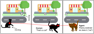
Figure 1: Stream with static and moving elements. The focus of attention (red circle) disambiguates what is observed, making the supervision well contextualized (2nd pic). The agent learns (1) pixel-wise representations that are coherent over the focused moving region, and (2) to make predictions (3rd pic). A stochastic sampling procedure yields an attention graph that facilitates learning.

In this paper, (i) we propose a novel approach to online learning from a video stream, that is rooted on the idea of using a scanpath-based focus of attention mechanism Zanca et al. (2020) to explore the video and to drive the learning dynamics in conjunction with motion information. The attention coordinates offer a precise location for interaction purposes, and its trajectory has been recently proved to efficiently select the most salient information of the video stream when learning with deep architectures Tiezzi et al. (2020). We propose to learn representations that are coherent over the temporal attention trajectory during slow movements of the simulated gaze, that are likely to cover visual patterns with the same semantics. Attention is paired with information coming from motion, that intrinsically suggests the spatial bounds of the attended area. This leads to a spatio-temporal unsupervised criterion that enforces coherence in the representations learned while observing what is moving (Fig. 1). In order to avoid trivial solutions, we augment the criterion with a contrastive term that favours the development of different representations in what is inside the moving area and what is right outside of it. Thanks to a graph-based formalization of this approach, we define a stochastic procedure that introduces variability in the information provided to the learning algorithm and leads to faster processing, also mitigating the effects of noisy motion information. (ii) We consider the case in which the human intervention is rare, and each supervision is about the coordinates of a single pixel with its class/instance label, thus not a signal that can strongly drive the features development. Target classes are not known in advance, and our model includes an open-set approach to avoid making predictions about unknown elements. In order to cope with continual learning, we propose a template-based schema with a dynamic update procedure that is synchronous with the processed stream and efficiently handled by modern hardware. (iii) Dealing with this setting introduces the further challenge of how to evaluate the artificial agent. We exploit the growing activity in realistic 3D Virtual Environments Meloni et al. (2020), designing from scratch (and sharing) three ad-hoc streams with different visual difficulty levels. (iv) We compare the learned representations with those from state-of-the art pretrained models that exploited a massive supervision, showing that the latter are not as powerful as one might expect in the considered setting.

2 Related Work

Online, continual, open set learning.

An online learning model progressively learns from a stream of data, continuously adapting to every new processed input instance Hoi et al. (2018). In the specific case of continual learning (also known as life-long, continuous or incremental learning Parisi et al. (2019)), the goal of the agent is not fixed a priori but changes over time. In this paper, the goal of the agent is to learn to predict the class labels in every pixel of a video stream. Such goal is not fully defined in advance, since the agent becomes aware of classes in function of what the human supervisor tells him, being closer to task-free cases Aljundi et al. (2019). Open-set classifiers Scheirer et al. (2012) can distinguish between examples belonging to different training classes and they can detect whether data do not belong to any of them, that is the case of what we propose. Our work is class-incremental Geng et al. (2020), due to the progressive inclusion of new classes after human intervention.

Focus of attention.

Several attempts to model human-like focus of attention mechanisms were presented Borji and Itti (2012), that not only differ in the way they are implemented, but also in the nature of the predicted attention (i.e., a temporal trajectory rather than saliency) Borji (2019). Recently, an unsupervised dynamical model was proposed Zanca et al. (2020) that can be applied both to static images and videos, also studied in the context of online learning in deep networks Tiezzi et al. (2020)—without any loss of generality, it is the model we consider here.

Learning invariant features.

Typical convolutional neural architectures require high sample complexity to learn representations invariant to factors that are not informative for the task at hand. Some solutions disentangle what and where features, each of them separately encoding informative and uninformative factors of variation Burt et al. (2021). This paper follows the perspective in which the attention trajectory, paired with motion information, offers a compact way to implicitly constrain the agent to learn invariances. This idea is linked to recent studies about learning invariance to motion in unsupervised learning over time Betti et al. (2020).

Semantic segmentation.

Semantic segmentation aims at associating a class label to each pixel of a given image. Deep architectures for this task usually rely on supervised learning from offline data, including fully convolutional networks Long et al. (2015), models based on transposed convolutions, dilated convolutions, upsampling and/or unpooling (U/V-net architectures Ronneberger et al. (2015)), transformers Ranftl et al. (2021). We will compare with these models.

Virtual environments.

The significantly improved quality of the rendered scenes and the intrinsic versatility of 3D Virtual Environments have quickly increased their popularity in the Machine Learning community (e.g., Gan et al. (2020)). SAILenv Meloni et al. (2020) is a recently proposed environment based on Unity3D, specifically aimed at easy customization and interface to Machine Learning libraries. SAILenv yields pixel-level motion information from Unity3D, and provides utilities to ease the generation of ad-hoc scenes for continual learning scenarios Meloni et al. (2021), making it well suited for what we propose.

3 Model

The basic concepts of the proposed unsupervised feature extractor are summarized in the example of Fig. 2. Our method is based on the assumption that a human-like attention trajectory Zanca et al. (2020) generally spans the important location of the stream, and the gaze moves more slowly within areas with uniform semantic properties, whose bounds can be further guessed by motion information. Hence, we enforce both temporal and spatial coherence constraints to force pixel embeddings to be consistent in time and space, with respect to locations virtually connected by the attention trajectory and by motion, respectively. We exploit a contrastive loss to avoid trivial solutions, and a stochastic approach to lighten the computational burden. Given the pixel embeddings, a template-based classifier learns how to classify each of them in an open-set class-incremental setting (Fig. 3).

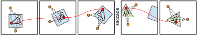
$t=0$          $t=1$          $t=2$          $t=3$          $t=4$

Figure 2: A rectangle rotates toward the right, attracting the attention $a_{t}$ (red nodes) that explores it. Then, a triangle enters the scene, and the simulated gaze quickly moves on it (saccade). The red path links nodes on which we enforce temporal coherence (not in saccades). For each $t$, some coordinates (yellow) are sampled in the moving region that includes $a_{t}$, while other points (orange) are sampled outside of it. Solid lines (positive edges) link spatially coherent samples; dashed lines (negative edges) are about the contrastive term.

Let us indicate with $X$ the set $\mathbb{R}^{w\times h\times c}$, and consider a continuous and potentially life-long video stream $V\in(X)^{\mathbb{N}}$ that, at the discrete time index $t\in\mathbb{N}\mapsto V_{t}\in X$, yields the video frame $V_{t}$ at the resolution of $w\times h$ pixels with $c$ channels. We also consider a neural network model that implements the function $f(\cdot,\omega)\colon X\rightarrow F$, with $F=\mathbb{R}^{w\times h\times d}$, where $\omega$ indicates the weights and biases of the net. The network is designed to process a frame $V_{t}$, and $f(V_{t},\omega)$ is an encoded representation of the frame where, for each pixel, we have a vector with $d$ components (Fig. 3). The network evolves over time and $\omega_{t}$ are the weights and biases at time $t$. We denote with $f_{x}$ the output of $f$ restricted to the pixel at 2D coordinates $x\in Z^{\diamond}:=\{1,\dots,w\}\times\{1,\dots,h\}$. In online learning from a video stream $V$, the network weights $\omega_{t+1}$ are obtained updating the previous $\omega_{t}$ with a law that depends on the gradient of a suitable loss function $L$ with respect to $\omega$.

Human-like attention.

The first pillar sustaining our model is a function $t\mapsto a(t)$, yielding an explicit estimate of the 2D coordinates where human would focus the attention at each time $t$. Among the various attention-prediction models yielding temporal trajectories Borji and Itti (2012), the recent unsupervised model Zanca et al. (2020) achieved state-of-the art results in simulating human-like attention. The authors showed that visual cues of the frame can act as gravitational masses. The equation of the potential of the gravitational field, $\varphi(x,t):=-{{(2\pi)}^{-1}}\int_{Z}\log\|x-z\|\mu(z,t)\,dz$, is at the basis of the attention model, where $Z$ is the continuous set of frame coordinates and $\mu(x,t)$ is the total mass at $(x,t)$. In particular, the magnitude of the brightness and an optical-flow-based measure of motion activity can be modeled as masses, and their impact is controlled by two positive scalars $\alpha_{b}$ and $\alpha_{m}$, respectively, and an inhibitory signal is also included. The focus of attention is modeled as a point-like particle subject to the above potential, and its trajectory $a(t)$ is determined integrating the following equation with initial conditions $a(0)=a^{0}$ and $\dot{a}(0)=a^{1}$,

$$\ddot{a}(t)+\rho\dot{a}(t)+\nabla\varphi(a(t),t)=0\qquad t>0,$$ (1)

where the dissipation is controlled by $\rho>0$ and $\nabla\varphi$ is the spatial gradient of the potential. The gaze performs fixations in locations of interest, with relatively low speed movements. Smooth pursuit consists of slow tracking movements performed to follow a considered stimulus. Differently, saccades are fast movements to relocate the attention toward a new target. In the most naive case, the first two categories of patterns can be distinguished by the latter exploiting a thresholding procedure on velocity, based on $\nu>0$.

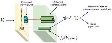
Figure 3: Pixels of frame $V_{t}$ are encoded into new representations by the neural net $f$. Inference involves all the coordinates (example for $x$), and the classifier $c$ can predict one or more classes or nothing (open-set). Classes are not known in advance. Learning is only about the attended moving area, developing coherent representations over time and space.

Temporal coherence.

During fixations, the attention spans a certain part of an object, with limited displacements of the gaze. Similarly, during smooth-pursuit the attended moving area has uniform semantic properties. Differently, during saccades, the attention switches the local context, shifting toward something that might or might not belong to the same object. We implement the notion of temporal coherence defining the loss function $L_{T}$ that ($i.$) restricts learning to the attention trajectory, filtering out the information in the visual scene Tiezzi et al. (2020) and ($ii.$) avoids abrupt changes in the feature representation during fixations and smooth pursuit,

$$L_{T}(\omega,\hat{\omega},t):=\delta_{t}\left\|f_{a_{t}}(V_{t},\omega)-f_{a_{t-1}}(V_{t-1},\hat{\omega})\right\|^{2},$$ (2)

where $\|\cdot\|$ is the Euclidean norm, and $\delta_{t}$ is equal to $0$ in case of saccades, otherwise it is $1$. When plugged into the online optimization, $\omega\leftarrow\omega_{t}$ and $\hat{\omega}\leftarrow\omega_{t-1}$. This loss is forced to zero for $t=0$, and it will be paired with other penalties described in the following, thus avoiding trivial solutions.

Spatial coherence.

Temporal coherence is not enough to capture the spatial extension of the encoded data, since it is only limited to the attention trajectory. Motion naturally provides such spatial information, and we follow this intuition designing agents that learn by observing moving attended regions. As a matter of fact, motion plays a twofold role, being crucial in defining the attention masses and as a mean to extend the notion of coherence to a frame region, i.e., spatial coherence. Formally, for each fixed $t\in\mathbb{N}$, we indicate with $S_{t}\subseteq Z^{\diamond}$ the set of frame coordinates that belong to the region of connected moving pixels that includes $a_{t}$. We introduce what we refer to as spatial attention graph at $t$, $\mathcal{G}_{t}$, with a node for each pixel of the frame ($\forall x\in Z^{\diamond}$) and with two types of edges, referred to as positive and negative edges. Positive edges link pairs of nodes whose coordinates belong to $S_{t}$, while negative edges link nodes of $S_{t}$ to nodes outside the moving region. The positive edges of the attention graph allow us to introduce a spatial coherence loss $L_{S}$,

$$L_{S}(\omega,t):=\frac{1}{2}\hskip-14.22636pt\sum_{\hskip 14.22636pt\begin{subarray}{c}x,z\in S_{t},x\neq z\end{subarray}}\hskip-14.22636pt\left\|f_{x}(V_{t},\omega)-f_{z}(V_{t},\omega)\right\|^{2},$$ (3)

that encourages the agent to develop similar representations inside the attended moving area $S_{t}$, while $\omega\leftarrow\omega_{t}$. The notion of learning driven by the fulfilment of spatio-temporal coherence over the attention trajectory ($L_{S}$ and $L_{T}$ of Eq. 2 and Eq. 3) is the second pillar on which our model is built.

Contrastive loss.

In order to prevent the development of trivial constant solutions, which fulfill the spatio-temporal coherence, we add a contrastive loss $L_{C}$ that works the opposite way $L_{S}$ does. In particular, $L_{C}$ exploits negative edges of $\mathcal{G}$ to foster different representations between what is inside the moving area and what is outside of it,

$$L_{C}(\omega,t):={\left(\hskip-14.22636pt\sum_{\hskip 14.22636ptx\in S_{t},z\in O_{t}}\hskip-19.91692pt\left\|f_{x}(V_{t},\omega)-f_{z}(V_{t},\omega)\right\|^{2}+\hskip-1.42262pt\varepsilon\right)^{-1}},$$ (4)

where $O_{t}=Z^{\diamond}\setminus S_{t}$ is composed of frame coordinates not in $S_{t}$ and $\varepsilon>0$ avoids divisions by zero. We notice that this contrastive loss is different from InfoNCE Oord et al. (2018).

Stochastic coherence.

These spatial and contrastive losses are plagued by two major issues. First, the number of pairs in Eq. 3 and Eq. 4 is large, being it $(1/2)|S_{t}|(|S_{t}|-1)$ and $|S_{t}|(wh-|S_{t}|)$, respectively, making the computation of the loss terms pretty cumbersome. Secondly, whenever an exact copy of a moving object appears in a not-moving part of the scene, there will be pixels of the first instance that are fostered to develop different representations with respect to pixels of the second one, what we refer to as collision. However, this clashes with the idea of developing a common representation of the object pixels. Hence, we replace $\mathcal{G}_{t}$ with the subgraph $\tilde{\mathcal{G}}_{t}$, that is the stochastic spatial attention graph at time $t$, composed by nodes that are the outcome of a stochastic sub-sampling of those belonging to $\mathcal{G}_{t}$. In particular, the node set of $\tilde{\mathcal{G}}_{t}$ is the union of $\tilde{S}_{t}\subseteq S_{t}$ and $\tilde{O}_{t}\subseteq O_{t}$, where $a_{t}$ is guaranteed to belong to the former. Edges of $\tilde{\mathcal{G}}_{t}$ are the positive and negative edges of $\mathcal{G}_{t}$ connecting the subsampled nodes. The key property of the stochastic graph is that the number of positive and negative edges is a chosen $e>0$. The set $\tilde{S}_{t}$ is populated by uniformly sampling nodes in $S_{t}$, ensuring that $a_{t}$ is always present, while $\tilde{O}_{t}$ is populated by sampling from a Gaussian distribution centered in $a_{t}$ and with variance $\sigma$, discarding samples $\notin O_{t}$. Large $\sigma$’s lead to sampling data also far away from the focus of attention, while small $\sigma$’s will generate samples close to the boundary of the moving region. In the example of Fig. 2 we emphasized how the attention bridges multiple instances of $\tilde{\mathcal{G}}_{t}$ over time, yielding a stochastic attention graph. Such a graph reduces the probability of collisions, both due to the random sampling and to the control on the sampled area by means of $\sigma$, and it introduces variability in the loss functions also when computed on consecutive frames. Moreover, the impact of imperfect segmentation of the moving region is reduced, since only some pixels are actually exploited, re-sampled at every frame. Since the number of pairs is bounded, the stochastic graph makes the formulation suitable for real-time processing.

Cumulative loss.

We define $L$ as the cumulative loss at a certain time instant $t$, where the contributes of Eq. 2, Eq. 3, Eq. 4 are weighted by the positive scalars $\lambda_{T}$, $\lambda_{S}$ and $\lambda_{C}$,

$$L(\omega,\hat{\omega},t):=\lambda_{T}L_{T}(\omega,\hat{\omega},t)+\lambda_{S}\tilde{L}_{S}(\omega,t)+\lambda_{C}\tilde{L}_{C}(\omega,t).$$ (5)

The losses $\tilde{L}_{S}$ and $\tilde{L}_{C}$ are the stochastic counterparts of $L_{S}$ and $L_{C}$, respectively, in which the sets $\tilde{S}_{t}$ and $\tilde{O}_{t}$ are used in place of $S_{t}$ and $O_{t}$. We define $\nabla L$ to be the gradient of the loss with respect to its first argument, that drives the online learning process, $\omega_{0}=\varpi,\ \omega_{t+1}=\omega_{t}-\alpha\nabla L(\omega_{t},\omega_{t-1},t),\ t\in\mathbb{N}$, with $\alpha>0$ (learning rate) and $\varpi$ some random initialization of the parameters of the network. We remark that other recent learning schemes for temporal domains could be exploited as well Tiezzi et al. (2020).

Pixel-wise classification.

A human supervisor occasionally provides a supervision at coordinates $a_{t}$ about a certain class $y_{t}$. Let us define an open-set classifier $c(\cdot,\xi,\zeta)\colon F\mapsto Q$ that predicts the class-membership scores (belonging to a generic set indicated with $Q$), over a certain number of classes that can be attached to each pixel-level representation. The main parameters of the classifier are collected in $\zeta$, and when all the membership scores are below threshold $\xi$ the classifier assumes to be in front on an unknown visual element and it does not provide a decision (open-set)—see Fig. 3. Whenever a supervision on a never-seen-before class is received, the classifier becomes capable of computing the membership score of such class for all the following time steps (class-incremental). We consider the case in which supervisions are extremely rare, not offering a suitable basis for gradient-based learning of $c$ or further refinements of $f$. The previously described unsupervised learning process is what is crucial to learn compact representations that can be easily classified, since it favours pixels of the same object to be represented in similar ways over time and space.

The most straightforward way to implement the open-set $c$ is with a distance-based model, storing the feature vectors associated to the supervised pixels as templates. This allows the model to not make predictions when the minimum distance from all the templates is greater than $\xi$. We indicate with $(k_{t},y_{t})$ a supervised pair where $k_{t}=f_{a_{t}}(V_{t},\omega_{t})$ is the template at coordinates $a_{t}$ of frame $V_{t}$. The intrinsic dependence of $k_{t}$ on the time index could make templates become outdated during the agent life, for example due to the evolution of the system, so that for some $t^{\prime}>t$ we might have $\|k_{t}-f_{a_{t}}(V_{t},\omega_{t^{\prime}})\|\gg 0$, leading to potentially wrong predictions. In order to solve this issue, we propose to dynamically update the templates. Modern hardware and software libraries for Machine Learning are designed to efficiently exploit batched computations In online learning, this feature is commonly not exploited, since only one data sample becomes available for each $t$. We indicate with $B_{t}$ a special type of mini-batch of frames, $B_{t}=\{V_{t}\}\cup\{V_{r},\ r\in H_{t}\}$, composed of the current $V_{t}$ and the frames associated to supervised time instants whose indices are in $H_{t}$. Due to the tiny number of supervisions, storing supervised frames does not introduce any critical issues, and a maximum size $b>1$ for each mini-batch can also be defined, populating $B_{t}$ with up to $b-1$ previously supervised frames, chosen with or without priority. This way, batched computations can be efficiently exploited to keep templates up-to-date.

4 Experiments

In order to create the right setting to evaluate what we propose, we need continuous streams able to provide pixel labels at spatio-temporal coordinates that are not defined in advance.

Virtual environments.

We consider photo-realistic 3D Virtual Environments within the SAILenv platform Meloni et al. (2020), that include pixel-wise semantic labeling and motion vectors of potentially endless streams, creating (from scratch) three 3D scenes to emphasize different and challenging aspects on which we measure the skills of the agents.. The agent observes the scene from a fixed location, and some objects of interest move, one at the time, along pre-designed smooth trajectories while rotating and getting closer to/farther from the camera. We denote with the term lap a complete route traveled by each object to its starting location.

We designed three different scenes. (i) EmptySpace: four photo-realistic textured object from the SAILenv library (chair, laptop, pillow, ewer) move over a uniform background. The goal is to distinguish them in a non-ambiguous setting. (ii) Solid: a gray-scale environment with three white solids (cube, cylinder, sphere) is considered. Due to the lack of color-related features, the agent must necessarily develop the capability of encoding information from larger contexts around each pixel. (iii) LivingRoom: the objects from EmptySpace are placed in a photo-realistic living room composed by other non-target objects (i.e., an heterogeneous background with a couch, tables, staircase, door, floor), and multiple static instances of the objects of interest. Samples of are shown in Fig. 4 (top) and, in what follows, $n$ is the number of target objects in each stream, while $m=n+1$ is the total number of categories (including the “unknown” class).

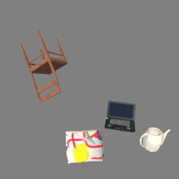
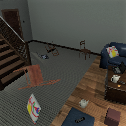
EmptySpace             Solid               LivingRoom

 $e=1\,$k, $\beta=1$    $e=20\,$k, $\beta=1$    $e=20\,$k, $\beta=5$

Figure 4: Top: sample frames from the three 3D scenes/streams (objects rotate and scale while moving). Bottom: samples of stochastic spatial graphs in EmptySpace (same color patterns of Fig. 2).

Setup.

We created three pre-rendered 2D visual streams by observing the moving scenes ($256\times 256$ pixels, with $\approx 51\,$k, $12\,$k and $20\,$k frames, respectively, corresponding to $31$ completed laps for each object), both in grayscale (BW) and color (RGB)—Solid is BW only. The agent learns by watching the first $25$ laps per object and, only in the subsequent laps, receives a total of $3$ supervisions $(k_{t},y_{t})$ per object, spaced out by at least $100$ frames. Learning stops when all the objects complete $30$ laps and, finally, performances are measured in the the last lap, considering the F1 score (averaged over the $m$ categories), either along the attention trajectory or in the whole frame area. We evaluated the proposed approach considering two different families of deep convolutional architectures yielding $d$ output features, referred to as HourGlass ( UNet-like Ronneberger et al. (2015)) and FCN-ND (6-layer Fully-Convolutional without any downsamplings Sherrah (2016)), respectively (see the supplementary material for all the details). We compared the obtained features against those produced by massively pretrained state-of-the-art models in Semantic Segmentation. We considered the Dense Prediction Transformer (DPT) Ranftl et al. (2021) and DeepLabV3 Chen et al. (2017) with ResNet101 backbone, exploiting both the features produced by the penultimate layer in the classification heads (-C suffix) and the ones obtained by the backbones (i.e., upsampling the representations if needed, -B suffix). In this way, we investigate both lower-level features based on backbones pretrained on millions of images (ImageNet), and task-specialized higher-level features for semantic segmentation (COCO Lin et al. (2014) and ADE20k Zhou et al. (2019) datasets—the latter explicitly includes the categories of the considered textured objects). As Baseline model we considered the case in which the pixel representations are left untouched (i.e., pixel color/brightness).

Parameters.

Parameters of the attention model were either fixed ($\alpha_{m}=1$), or adapted according to a preliminary run of the model ($\alpha_{b}$, $\rho$). For each video stream, we searched for the model hyper-parameters that maximize the F1 along the attention trajectory, measured during the $30$-th laps (hyper-params grids and the best selected are reported in the suppl. material). Fig. 4 (bottom) shows the effects of the parameters $e$ and $\beta$ in modeling the stochastic coherence graph.

Results.

Table 1 (top) shows the F1 along the attention trajectory measured during the latest object lap, averaged over 3 runs with different initialization. The proposed learning mechanism is competitive and able to overcome models pretrained on large supervised data. This is mostly evident in the case of HourGlass, while FCN-ND is less accurate, mostly due to the lack of implicit spatial aggregation. Table 1 (bottom) is about the F1 computed considering predictions on all the pixels of all the frames. This measure is not directly affected by the attention model, and while our model performs worse, it is still on par with some of the competitors, with the exception of LivingRoom (RGB).

	EmptySpace		Solid	LivingRoom
	BW	RGB	BW	BW	RGB
DPT-C	$0.70$	$0.76$	$0.54$	$0.38$	$0.39$
DPT-B	0.73	0.77	$0.53$	$0.29$	$0.32$
DeepLab-C	$0.46$	$0.57$	$0.56$	$0.19$	$0.26$
DeepLab-B	$0.61$	$0.72$	$0.66$	$0.28$	$0.35$
Baseline	$0.39$	$0.61$	$0.32$	$0.52$	0.65
HourGlass	0.73 $\pm 0.03$	0.77 $\pm 0.05$	0.68 $\pm 0.02$	0.59 $\pm 0.02$	$0.45$ $\pm 0.12$
FCN-ND	$0.69$ $\pm 0.03$	$0.57$ $\pm 0.08$	$0.58$ $\pm 0.07$	$0.39$ $\pm 0.02$	$0.38$ $\pm 0.02$
DPT-C	$0.66$	$0.67$	$0.64$	$0.35$	$0.39$
DPT-B	0.71	$0.69$	0.68	0.39	$0.39$
DeepLab-C	$0.49$	$0.61$	$0.57$	$0.31$	$0.34$
DeepLab-B	$0.70$	$0.65$	$0.66$	$0.34$	0.44
Baseline	$0.50$	$0.45$	$0.18$	$0.10$	$0.23$
HourGlass	$0.55$ $\pm 0.03$	0.71 $\pm 0.03$	$0.50$ $\pm 0.01$	$0.31$ $\pm 0.04$	$0.25$ $\pm 0.07$
FCN-ND	$0.60$ $\pm 0.05$	$0.51$ $\pm 0.07$	$0.48$ $\pm 0.03$	$0.24$ $\pm 0.01$	$0.28$ $\pm 0.03$

Table 1: Top: F1 score (mean $\pm$ std) measured along the attention trajectory. Competitors are not affected by the model initialization (no std). Bottom: F1 considering all the pixels.

We investigated our results, showing in Fig. 5 some sample predictions comparing HourGlass with transformers (DPT-B). Indeed, state-of-the-art models have troubles in recognizing closer objects and also in discriminating from the background, due to the fact that their pixel representations are typically strongly affected by a large context. When presenting objects in unusual orientations, likely different from what observed during the fully supervised training, they tend to perform badly. Differently, our model adapts to the video stream, learning more coherent representations when the object transforms. Overall, the attention model allows to focus on what is more important, and, although just a tiny number of supervisions are provided, our model can online-learn to make predictions that competes with the massively offline trained competitors.

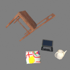
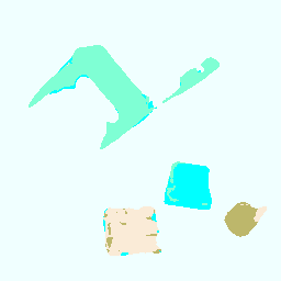
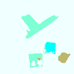
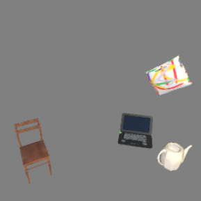
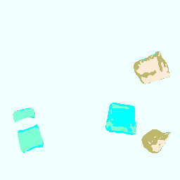
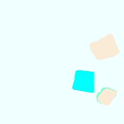
  Frame               HourGlass               DPT-B

Figure 5: Predictions in two frames, comparing HourGlass (our) with DPT-B (transformers) in EmptySpace stream. Different colors indicate different predictions.

In-depth studies and ablations.

In order to evaluate the sensitivity of the proposed approach to the key elements of the considered setup, we selected the HourGlass model of Table 1. Fig. 6 reports results of experiments in which we changed the number of supervisions per object, the number of edges $e$ (per type) in the stochastic graph, we disabled the temporal coherence, and we changed the length of the streams (discarding Solid in which differences were less appreciable). Even with a single supervision, the model is able to distinguish the target objects in EmptySpace, while in the more cluttered LivingRoom it benefits from multiple supervisions, as expected. Our proposal is better than using a non-stochastic criterion (LivingRoom), and works well even with a limited value for $e$. Moreover, the agent benefits from relatively longer streams (going from 15 to 30 laps), that allow it to develop more coherent representations (we tuned the model in the 30-lap case, that is the reason for the slight performance drop in 55-lap), and temporal coherence has an important role in the overall results. For completeness, we highlighted in Fig. 6 (last) the computational benefits, in terms of time (one lap per object), brought by the stochastic subsampling, showing that they are more evident for large $d$.

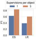
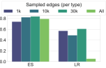
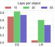
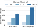
Figure 6: First 4 plots (left-to-right, top-to-bottom): in-depth experiments on EmptySpace (ES) and LivingRoom (LR) RGB streams (F1 on focus trajectory). Last plot: timings (3 runs) for stochastic sampling ($e=10\,$k) and no subsampling at all, varying $d$.

5 Conclusions

We presented a novel approach to the design of agents that continuously learn from a visual environment dealing with an open-set class-incremental setting, leveraging a focus of attention mechanism and spatio-temporal coherence. We devised an innovative way of benchmarking this class of algorithms using 3D Virtual Environments, in which our proposal leads to results that, on average, are comparable to those obtained using state-of-the art strongly-supervised models.

Supplemental Material
  

This supplemental paper includes more details about some aspects of the main paper. Moreover, it provides full references to our code, to the instructions to reproduce our results (including all the selected hyperparameters), and, more importantly, to the 3D scenes that we created for this activity. Such scenes are plugged into the 3D Virtual Environment named SAILenv Meloni et al. [2020], for which we provide further references and instructions. The same scenes were also pre-rendered, saving frames, pixel-wise labels, and optical flow to disk—we are also sharing these data.

Notice that the bibliographic references in this supplemental paper are about the bibliography of the main paper.

Appendix A Normalized Representations

In addition to what has been described in the main paper, we also explored the case in which the feature vectors are normalized in order to have unitary Euclidean norms,

$$\|f_{x}(V_{t},\omega_{t})\|=1,\quad\forall x\in Z^{\diamond},\quad\forall t\geq 0.$$ (6)

This avoids the system to encode information in the length of the feature vectors, and it can be used to simplify the loss terms of Eq. 2, Eq. 3, Eq. 4 as follows,

$$L_{T}(\omega,\hat{\omega},t)\hskip-5.69054pt := \hskip-5.69054pt\delta_{t}\left(1-\langle f_{a_{t}}(V_{t},\omega),f_{a_{t-1}}(V_{t-1},\hat{\omega})\rangle\right)$$ (7)

$$L_{S}(\omega,t)\hskip-5.69054pt := \hskip-5.69054pt\frac{1}{2}\sum_{\begin{subarray}{c}x,z\in S_{t}\\ x\neq z\end{subarray}}\left(1-\langle f_{x}(V_{t},\omega),f_{z}(V_{t},\omega)\rangle\right)$$ (8)

$$L_{C}(\omega,t)\hskip-5.69054pt := \hskip-8.53581pt\sum_{x\in S_{t}}\sum_{z\in O_{t}}\left(1+\langle f_{x}(V_{t},\omega),f_{z}(V_{t},\omega)\rangle\right)$$ (9)

where $\langle\cdot,\cdot\rangle$ is the dot product and each loss has zero as minimum value. In the case of pixel-wise classification, when using normalized representations we computed the distance between a template $k_{t}$ and a certain feature vector $f_{x}(V_{t^{\prime}},\omega_{t^{\prime}})$ (with $t^{\prime}\geq t$) as

$$\texttt{dist}\left(k_{t},f_{x}(V_{t^{\prime}},\omega_{t^{\prime}})\right)=1-\langle k_{t},f_{x}(V_{t^{\prime}},\omega_{t^{\prime}})\rangle,$$ (10)

and the open-set threshold $\xi$ belongs to $(0,2]$.

Appendix B Segmenting the Attended Moving Region

The coordinates belonging to set $S_{t}$ are those of the pixels that belong to the moving region that includes the attention coordinates $a_{t}$. If $v_{x,t}$ is the 2D velocity of pixel at coordinates $x$ and time $t$, then such pixel is a moving pixel if and only if it is associated to a non-vanishing optical flow, i.e.,

$$\|v_{x,t}\|>\gamma,$$ (11)

given $\gamma>0$ and being $\|\cdot\|$ the Euclidean norm. Two moving pixels that are direct neighbors in the image plane are defined as connected, and a chain of connected pixels implements what we will refer to as a path. We introduce the function $\texttt{path\_exists}(x,a_{t})$, that returns true if there exists a path connecting $x$ to the attention $a_{t}$. Hence,

$$S_{t}=\{x\colon\texttt{path\_exists}(x,a_{t})\}\cup\{a_{t}\}.$$ (12)

If there are no moving pixels in the current frame, then we consider $S_{t}$ to be empty (in this case, also $a_{t}\notin S_{t}$), and the spatial coherence and contrastive losses are set to zero.

In order to segment the moving area as defined above, we implemented a frontier-based algorithm reported in Alg. 1, where the function neighbors(x) returns the set of direct neighbors of $x$.

Algorithm 1 Determining the moving area that includes the focus of attention.

0:  Optical flow $\left[v_{x,t}\right]_{x\in Z^{\diamond}}$, attention coordinates $a_{t}$, threshold $\gamma>0$.

0:  Set of coordinates belonging to the moving area, i.e., $S_{t}$.

1:  $S_{t}\leftarrow\{a_{t}\}$ {$\triangleright$ initial set}

2:  $\mathcal{F}\leftarrow\{a_{t}\}$ {$\triangleright$ initial frontier}

3:  while $\mathcal{F}\neq\emptyset$ do

4:     $\mathcal{N}\leftarrow\cup_{x\in\mathcal{F}}\texttt{neighbors}(x)$ {$\triangleright$ union of the neighbors of the points in the frontier}

5:     $\mathcal{F}\leftarrow\{z:z\in\mathcal{N}\land z\notin S_{t}\land\|v_{z,t}\|>\gamma\}$ {$\triangleright$ new frontier: moving pixels in $\mathcal{N}$ (not in $S_{t}$)}

6:     $S_{t}\leftarrow S_{t}\cup\mathcal{F}$ {$\triangleright$ adding the new frontier to $S_{t}$}

7:  end while

8:  if $|S_{t}|=1$ then

9:     $S_{t}\leftarrow\emptyset$ {$\triangleright$ if only $a_{t}$ belongs to $S_{t}$, we clear it}

10:  end if

11:  return  $S_{t}$

Appendix C Setup

We created three visual streams ($256\times 256$), both in grayscale (BW) and color (RGB)—Solid is BW only—by observing the moving scenes. To accelerate the experimental validation we generated $\approx 51\,$k, $12\,$k and $20\,$k pre-rendered frames from the three aforementioned streams, respectively, that correspond to $31$ completed laps for each object. The agent learns by watching the first $25$ laps per object and, afterwards, he receives $3$ supervisions $(k_{t},y_{t})$ per object at different time instants, starting from the first frame of the route and waiting at least $100$ frames before supervising the same object again (of course, $a_{t}$ must belong to the supervised object, and we set $b=1+3n$ to ensure a frequent update of the templates). When all the objects complete $30$ laps, we stopped learning the model parameters and, finally, the last lap was the one on which performance is measured.

Parameters.

The parameters of the attention model were either fixed ($\alpha_{m}=1$), or adapted according to a preliminary run of the model on the video streams ($\alpha_{b}$, $\rho$). For each video stream, we searched for the model hyper-parameters that maximize the F1 along the attention trajectory, measured during the $30$-th laps, considering the following grids: $\alpha\in\{5\cdot 10^{-6},10^{-4},5\cdot 10^{-4},10^{-3}\}$, $\lambda_{T}\in\{10^{-2},10^{-1},1\}$, $\lambda_{S}\in\{10^{-4},10^{-3},10^{-2}\}$, $\lambda_{C}\in\{10^{-4},10^{-2},10^{-1},1,10\}$, $d\in\{32,128\}$, $e\in\{5\,\text{k},10\,\text{k},30\,\text{k}\}$, $\beta\in\{3,5\}$. For simplicity, we assumed the model to be aware of the optimal open-set threshold $\xi$, that we found by searching on a dense grid. Fig. 4 (bottom) shows the effects of the parameters $e$ and $\beta$ in modeling the stochastic coherence graph.

Appendix D Neural Architectures

Our models.

The experimental campaign was carried out evaluating the performance of the proposed approach using two different types of deep convolutional architectures with $d$ output filters, referred to as HourGlass and FCN-ND, respectively. The former is a UNet Ronneberger et al. [2015] architecture based on a ResNet18 backbone. We explored several architectural variations for this model, including the removal of Batch Normalization (that in our setting boils down to spatial normalization since we process frames one after the other) from the whole structure and by removing some skip connections. Indeed, differently from what commonly happens in supervised Semantic Labeling where a target is defined on each pixel, in our case, due to the unsupervised criterion, the presence of skip connections could induce the model to not consider the inner portions of the network, developing representations that are extremely local in terms of spatial information that they encode. This fact could entail trivial solutions in datasets composed by simple objects characterized by several pixels with instance-specific colors, making the RGB information an attractive way for representing pixel-wise features. Hence, we tested some variations of the original implementation, either removing all the skip connections or only the one connecting the input with the output layer. We treated these variants of the HourGlass network as special hyperparameters of the model. Differently, the other model we considered, FCN-ND, is a 6-layer Fully-Convolutional model that maintains the same image-resolution throughout the whole architecture, without any downsamplings/poolings, inspired by Sherrah [2016]. It is based on $5\times 5$ filters, with 6 layers composed of 32 filters in each hidden layer, except from the first one, which contains $16$ filter banks. In the experiments, we report the average results obtained over 3 runs initialized with random seeds (torch.manual_seed in the PyTorch library, leveraging the time package). We report in Table 2 the hyperparameters corresponding to the best models. See the provided code repository for further details (e.g, on the network variations hyperparameters.)

		EmptySpace		Solid	LivingRoom
	Parameters	BW	RGB	BW	BW	RGB
HourGlass	$\alpha$	$5\cdot 10^{-6}$	$5\cdot 10^{-4}$	$10^{-4}$	$10^{-3}$	$5\cdot 10^{-4}$
	$\lambda_{T}$	1	1	$10^{-1}$	$10^{-1}$	$10^{-1}$
	$\lambda_{S}$	$10^{-4}$	$10^{-4}$	$10^{-3}$	$10^{-2}$	$10^{-3}$
	$\lambda_{C}$	$10^{-1}$	$10^{-1}$	$10^{-1}$	10	10
	$d$	32	128	128	32	32
	$e$	$30\,\text{k}$	$30\,\text{k}$	$10\,\text{k}$	$30\,\text{k}$	$30\,\text{k}$
	$\beta$	5	5	5	5	5
	Norm.	yes	yes	yes	yes	yes
FCN-ND	$\alpha$	$10^{-3}$	$10^{-3}$	$10^{-3}$	$10^{-4}$	$10^{-3}$
	$\lambda_{T}$	$10^{-1}$	$10^{-2}$	$10^{-2}$	$10^{-2}$	$10^{-2}$
	$\lambda_{S}$	$10^{-2}$	$10^{-3}$	$10^{-2}$	$10^{-2}$	$10^{-3}$
	$\lambda_{C}$	$10^{-2}$	$10^{-2}$	$10^{-2}$	1	$10^{-1}$
	$d$	32	32	32	128	128
	$e$	$10\,\text{k}$	$10\,\text{k}$	$10\,\text{k}$	$30\,\text{k}$	$30\,\text{k}$
	$\beta$	5	3	3	3	3
	Norm.	no	no	no	yes	yes

Table 2: Optimal parameters. Best selected hyperparameters drawn from the grid search described in the main text (see Section 4), both for HourGlass (top) and FCN-ND (bottom) architectures. Additionally, we denote with Norm. $\in\{yes,no\}$ the choice of processing normalized feature vectors (unitary norm) and not normalized ones, respectively. For further details, see the provided code repository.

Competitors.

DPT Ranftl et al. [2021] is a recently proposed architecture based on vision transformers as a backbone for dense prediction tasks, characterized by high resolutions processing and global receptive fields over the whole frame. We leveraged a pretrained implementation on the ADE20K dataset Zhou et al. [2019]. We exploited the best-performing model of Ranftl et al. [2021], that the authors named DPT-Hybrid. Differently, DeepLabv3 Chen et al. [2017] is based on multiple atrous convolutions rates in order to capture multi-scale contexts. We employed a model based on a ResNet101 backbone and finetuned on COCO dataset Lin et al. [2014].

Appendix E Code, 3D Scenes, Video Streams

This section contains full references to our code and the instructions to reproduce our results. At the following link: https://github.com/sailab-code/cl_stochastic_coherence the reader can find all that is needed to run the experiments. We include the code (PyTorch–Modified BSD license), data (MIT license) and the selected hyper-parameters. See the README file for further details on the archive contents and how to execute the code and on the mapping of the parameters name in the code – see the ”Argument description” in HOW TO RUN AN EXPERIMENT. Notice that the reproduce_runs.txt contains the command lines (hence, the best selected parameters) required to reproduce the experiments of the main results (also reported in Table 2 for completeness).

Moreover, we provide in the same repository (folder 3denv) the three visual scenes we created (EmptySpace, Solid, LivingRoom) for this activity, leveraging the 3D Virtual Environment named SAILenv Meloni et al. [2020]. In addition, the same scenes were pre-rendered into the three visual streams we exploited in the experimental section, saving frames, pixel-wise labels, and motion information to disk.

In the following, we will describe how to load such scenes into the SAILenv environment and the pre-rendered data folder structure.

Computing infrastructure.

The experimental campaign was mainly carried out on a machine equipped with Ubuntu 18.04.3 LTS, two NVIDIA Tesla V100-SXM2-32GB GPUs, Intel Xeon Silver 4110 (32 cores) @ 2.101GHz CPU, 48 GB of RAM. Additionally, a portion of the experiments was carried out on two other machines: the former one is equipped with Ubuntu 18.04.1 LTS, three NVIDIA 1080Ti-11GB GPUs, Intel i9-7900X (20 cores) @ 3.30GHz CPU, 128 GB of RAM. The latter one with Ubuntu 18.04.4 LTS, an NVIDIA GTX TITAN-6GB GPU, Intel i7-3970X (12 cores) @ 3.50GHz CPU, 64 GB of RAM.

We used Numpy (v1.19.5) for saving numerical arrays and We exploited the wandb platform to organize and track our experiments.

E.1 3D scenes

EmptySpace                           Solid                           LivingRoom

Figure 7: Sample frames from the three 3D scenes/streams (objects rotate and scale while moving). We report the same figures of the main paper (see Figure 4, top) in a bigger resolution, to better appreciate the visual stream details.

The scenes are available in the 3denv folder of the same repository (link https://github.com/sailab-code/cl_stochastic_coherence). The 3denv folder contains three .unity files and three associated directories.

• EmptySpace.unity: contains the scene named EmptySpace.

• Solid.unity: contains the scene named Solid.

• LivingRoom.unity: contains the scene named LivingRoom.

To install the scenes you must follow these instructions:

1. Download the latest SAILenv source code from SAILenv site (https://sailab.diism.unisi.it/sailenv/) and extract the files into a directory.

2. Download Unity 2019.4.2f1 from Unity website (https://unity3d.com/get-unity/download). Using Unity HUB is the easiest way. NOTE: to use Unity you will need to create an account with a personal free license (Unity Personal).

3. Open the SAILenv directory with Unity. The first time it will take around 15 minutes to fully load.

4. Copy the content of the scenes directory (3denv/scenes) into Assets/Scenes

5. Through the Unity Editor, open the file Assets/Settings/AvailableScenesSettings.

6. The Inspector will show a list of the available scenes. Change the textbox named Size from 4 to 7. This will create three new empty boxes that can be filled by dragging the scenes objects from the Project view to the scene box in the Inspector and assign names to the scenes in the textbox below (see Figure 8) (the scenes will be exposed through the Python API with these names - see the example scripts in the official site (https://sailab.diism.unisi.it/sailenv/).

   

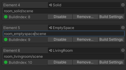
   Figure 8: Example on how to assign names to the scenes in the text box in Unity.

7. Press the Add (buildIndex N) and then confirm Add as enabled for each of the newly added scenes.

8. On the top bar, select SAILenv/Builds/Local AssetBundles. It will take a while to compile the resources.

9. Open the ”Main Menu” scene in Assets/Scenes and press the Play button on the top. There is no need to interact with this scene, just proceed to the next step.

10. The Environment is now running and you can use the Python API to open the new scenes through the names you have given.

The visual stream is made available to clients (default port 8085) by clicking on the play icon in Unity or by building and launching a standalone application. A brief snippet of code that uses the InputStream class (available in our source code) to fetch in real time the rendered stream is available in Figure 9. We report in Figure 7 a sample frame from each one of the processed visual streams.

⬇

import lve

\par# sailenv settings for the Solid scene

unity_settings = {

’depth_frame_active’: False,

’flow_frame_active’: True,

’object_frame_active’: False,

’main_frame_active’: True,

’category_frame_active’: True,

’use_gzip’: False,

’scene’: ’room_solid/scene’

}

\par# create InputStream object

ins = lve.InputStream(”localhost:8085”, w=256, h=256,

fps=8, repetitions=20,

force_gray=False,

unity_settings=unity_settings)

\par# set agent camera as grey solid background

agent = ins.get_unity_agent()

agent.change_main_camera_clear_flags(128, 128, 128)

\par# place agent into its default position for the scene

agent.toggle_follow()

\par# getting next frame, motion, supervision and foa traj.

img, of, supervisions, foa = ins.get_next()

\par

Figure 9: Code snippet to access the SAILenv scenes using the Python API and the provided InputStream class. Frame data are obtained with the .get_next() method.

E.2 Video Streams folders

We rendered the three scenes and extracted the corresponding visual streams described in Section 4. The data folder contains one subfolder for each one of such visual streams. The directory tree of each one of such folders (named after the streams name EmptySpace, Solid, LivingRoom) is composed as follows.

.foa file It is the output of the FOA (focus of attention) computation. The attention is stored in a CSV-like format: foa_x, foa_y, v_x, v_y, saccade, with Focus of Attention (FOA) frame coordinates and velocity, besides a boolean flag which is true if a saccade is detected for the current frame.

frames directory It contains the full-resolution frames, stored in PNG format in subfolders of 100 frames.

motion directory It contains the motion arrays (pixel-wise XY velocity, in $(w,h,2)$-shaped tensors), stored in NumPy format (gzip compressed, .bin extension) in subfolders of 100 frames.

sup directory It contains the frame-wise supervision arrays (targets and indices), both stored in NumPy format (gzip compressed, .bin extension) in subfolders of 100 frames. Such supervision is stored in a sparse manner, given the fact that we consider pixel-wise supervisions on the FOA coordinates $a_{t}$. targets contains the target class of the supervision for some pixels, while indices contains the raveled index of the corresponding supervised pixels.

Loading the pre-rendered scenes.

The InputStream class utility can be used to load into Python the prerendered scenes. Figure 10 contains a simple code example to load one of the streams and get some data from it. In particular, the get_next() method returns the next frame, its optical flow, pixel-wise supervisions and the coordinates attended by the Focus of Attention in that frame.

⬇

import lve

\par# precomputed FOA trajectory file

foa_file=”data/emptyspace/empty_space_bench_foa_long.foa”

# create InputStream object

ins = lve.InputStream(”data/emptyspace”, w=-1, h=-1,

fps=None, max_frames=None,

repetitions=1, force_gray=”yes”,

foa_file=foa_file)

\par# getting next frame, motion, supervision and foa traj.

img, of, supervisions, foa = ins.get_next()

\par

Figure 10: Loading the pre-rendered EmptySpace visual stream through the InputStream class and getting the data from the next frame using Python.

References

- Aljundi et al. [2019] Rahaf Aljundi, Klaas Kelchtermans, and Tinne Tuytelaars. Task-free continual learning. In Proc. of the IEEE/CVF CVPR, pages 11254–11263, 2019.
- Betti et al. [2020] Alessandro Betti, Marco Gori, and Stefano Melacci. Learning visual features under motion invariance. Neural Networks, 126:275–299, 2020.
- Borji and Itti [2012] Ali Borji and Laurent Itti. State-of-the-art in visual attention modeling. IEEE TPAMI, 35(1):185–207, 2012.
- Borji [2019] Ali Borji. Saliency prediction in the deep learning era: Successes and limitations. IEEE TPAMI, 2019.
- Burt et al. [2021] Ryan Burt, Nina N. Thigpen, Andreas Keil, and Jose C. Principe. Unsupervised foveal vision neural architecture with top-down attention. Neural Networks, 141:145–159, 2021.
- Chaudhari et al. [2019] Sneha Chaudhari, Varun Mithal, Gungor Polatkan, and Rohan Ramanath. An attentive survey of attention models. arXiv preprint arXiv:1904.02874, 2019.
- Chen et al. [2017] Liang-Chieh Chen, George Papandreou, Iasonas Kokkinos, Kevin Murphy, and Alan L Yuille. Deeplab: Semantic image segmentation with deep convolutional nets, atrous convolution, and fully connected crfs. IEEE TPAMI, 40(4):834–848, 2017.
- Gan et al. [2020] Chuang Gan, Jeremy Schwartz, Seth Alter, Martin Schrimpf, et al. Threedworld: A platform for interactive multi-modal physical simulation. arXiv:2007.04954, 2020.
- Geng et al. [2020] Chuanxing Geng, Sheng-jun Huang, and Songcan Chen. Recent advances in open set recognition: A survey. IEEE TPAMI, 2020.
- Hoi et al. [2018] Steven CH Hoi, Doyen Sahoo, Jing Lu, and Peilin Zhao. Online learning: A comprehensive survey. arXiv preprint arXiv:1802.02871, 2018.
- Jing and Tian [2020] Longlong Jing and Yingli Tian. Self-supervised visual feature learning with deep neural networks: A survey. IEEE TPAMI, 2020.
- Kornblith et al. [2019] Simon Kornblith, Jonathon Shlens, and Quoc V. Le. Do better imagenet models transfer better? In Proc. of the IEEE/CVF CVPR, June 2019.
- Lin et al. [2014] Tsung-Yi Lin, Michael Maire, Serge Belongie, James Hays, Pietro Perona, Deva Ramanan, Piotr Dollár, and C Lawrence Zitnick. Microsoft coco: Common objects in context. In ECCV, pages 740–755. Springer, 2014.
- Long et al. [2015] Jonathan Long, Evan Shelhamer, and Trevor Darrell. Fully convolutional networks for semantic segmentation. In Proc. of the IEEE/CVF CVPR, pages 3431–3440, 2015.
- Meloni et al. [2020] Enrico Meloni, Luca Pasqualini, Matteo Tiezzi, Marco Gori, and Stefano Melacci. Sailenv: Learning in virtual visual environments made simple. In ICPR, pages 8906–8913, 2020.
- Meloni et al. [2021] Enrico Meloni, Alessandro Betti, Lapo Faggi, Simone Marullo, Matteo Tiezzi, and Stefano Melacci. Evaluating continual learning algorithms by generating 3d virtual environments. arXiv preprint arXiv:2109.07855, 2021.
- Min et al. [2021] Juhong Min, Dahyun Kang, and Minsu Cho. Hypercorrelation squeeze for few-shot segmentation. arXiv preprint arXiv:2104.01538, 2021.
- Oord et al. [2018] Aaron van den Oord, Yazhe Li, and Oriol Vinyals. Representation learning with contrastive predictive coding. arXiv preprint arXiv:1807.03748, 2018.
- Parisi et al. [2019] German I Parisi, Ronald Kemker, Jose L Part, Christopher Kanan, and Stefan Wermter. Continual lifelong learning with neural networks: A review. Neural Networks, 113:54–71, 2019.
- Ranftl et al. [2021] René Ranftl, Alexey Bochkovskiy, and Vladlen Koltun. Vision transformers for dense prediction. CoRR, abs/2103.13413, 2021.
- Ronneberger et al. [2015] Olaf Ronneberger, Philipp Fischer, and Thomas Brox. U-net: Convolutional networks for biomedical image segmentation. In MICCAI, pages 234–241. Springer, 2015.
- Russell and Norvig [2009] Stuart Russell and Peter Norvig. Artificial Intelligence: A Modern Approach. Prentice Hall Press, USA, 3rd edition, 2009.
- Scheirer et al. [2012] Walter J Scheirer, Anderson de Rezende Rocha, Archana Sapkota, and Terrance E Boult. Toward open set recognition. IEEE TPAMI, 35(7):1757–1772, 2012.
- Sherrah [2016] Jamie Sherrah. Fully convolutional networks for dense semantic labelling of high-resolution aerial imagery. arXiv preprint arXiv:1606.02585, 2016.
- Tiezzi et al. [2020] Matteo Tiezzi, Stefano Melacci, Alessandro Betti, Marco Maggini, and Marco Gori. Focus of attention improves information transfer in visual features. In NeurIPS, volume 33, pages 22194–22204, 2020.
- Zanca et al. [2020] Dario Zanca, Stefano Melacci, and Marco Gori. Gravitational laws of focus of attention. IEEE TPAMI, 42(12):2983–2995, 2020.
- Zhou et al. [2019] Bolei Zhou, Hang Zhao, Xavier Puig, Tete Xiao, Sanja Fidler, Adela Barriuso, and Antonio Torralba. Semantic understanding of scenes through the ade20k dataset. IJCV, 127(3):302–321, 2019.