Broad Recommender System: An Efficient Nonlinear Collaborative Filtering Approach

Abstract

Recently, Deep Neural Networks (DNNs) have been largely utilized in Collaborative Filtering (CF) to produce more accurate recommendation results due to their ability of extracting the nonlinear relationships in the user-item pairs. However, the DNNs-based models usually encounter high computational complexity, i.e., consuming very long training time and storing huge amount of trainable parameters. To address these problems, we develop a novel broad recommender system named Broad Collaborative Filtering (BroadCF), which is an efficient nonlinear collaborative filtering approach. Instead of DNNs, Broad Learning System (BLS) is used as a mapping function to learn the nonlinear matching relationships in the user-item pairs, which can avoid the above issues while achieving very satisfactory recommendation performance. However, directly feeding the original rating data into BLS is not suitable due to the very large dimensionality of the original rating vector. To this end, a new preprocessing procedure is designed to generate user-item rating collaborative vector, which is a low-dimensional user-item input vector that can leverage quality judgments of the most similar users/items. Convincing experimental results on seven datasets have demonstrated the effectiveness of the BroadCF algorithm.

I Introduction

In the era of information explosion, the rich choices of online services lead to an increasingly heavy role for recommender systems (RSs). The goal of RSs is to recommend the preferable items to users based on their latent preferences extracted from the historical behavioral data [1, 2, 3, 4, 5, 6, 7, 8, 9, 10, 11]. Collaborative filtering is one of the most classical recommendation algorithms, which has been widely used in many real-world tasks [12, 13, 14, 15, 16, 17].

The traditional collaborative filtering is user-oriented or item-oriented, which relies mainly on the rating information of similar users or items to predict unknown ratings. Among various collaborative filtering techniques, Matrix Factorization (MF) [18, 19, 20, 21] is the most popular approach, which operates by learning the latent representations of users/item in the common space. In the common space, the recommender system predicts the rating of the user-item pair based on their latent representations. However, in practical applications, scoring data is prone to long-tail distribution [22], which can lead to the sparsity problem in the MF methods. To overcome the sparsity problem, several methods have been developed [23], e.g., adding social relations to MF or using invisible feedback [24].

Deep Neural Networks (DNNs) have been rapidly developed recently, which have shown satisfactory results in different fields such as computer vision and natural language processing. DNNs have also been introduced into the field of RSs [25, 26, 27, 28, 29, 30]. In the traditional matrix decomposition, the relationships in the user-item pairs are usually assumed to be linear, which is however not true in real-world scenarios. To better learn nonlinear matching relationships in the user-item pairs, Xue et al. propose Deep Matrix Factorization (DMF) [26] that leverages a dual-path neural network instead of the linear embedding adopted in the conventional matrix decomposition. DNNs are able to approximate any function, so they are well suitable for learning complex matching functions. For example, He et al. propose the Neural Collaborative Filtering (NCF) framework [27], which takes as input the concatenation of user-item embeddings and uses Multi-Layer Perceptron (MLP) for prediction. Deng et al. propose DeepCF [31] which is a unified deep collaborative filtering framework integrating matching function learning and representation learning. However, the above DNNs-based models require a large number of training epochs that are computationally expensive, and therefore cannot be applied to large-scale data and are very time consuming. As shown in our experiments, due to the out-of-memory error, most DNNs-based models fail to generate results when dealing with an Amazon dataset containing 429622 users, 23966 items, and 583933 ratings on a server with an Intel Core i9-10900 CPU, GeForce RTX 3090, and 256GB of RAM. And even for the relatively small datasets that can generate results, most DNNs-based models are time-consuming. In [29], a BP Neural Network with Attention Mechanism (BPAM) has been developed to mitigate this problem by combining attention mechanism with the BP network. However, the gradient-based optimization still consumes long time.

To address the aforementioned problems, this paper proposes a novel broad recommender system, called Broad Collaborative Filtering (BroadCF), which is an efficient nonlinear collaborative filtering approach. Different from the DNNs-based methods that feed the user-item rating data into DNNs, the proposed BroadCF method feeds the user-item rating data into Broad Learning System (BLS) [32]. As shown in the literature [32, 33], BLS is also able to approximate any function, and its general approximation capability has been theoretically analyzed at the beginning of its design and proved by rigorous theoretical proof. In particular, it can map the data points to a discriminative space by using random hidden layer weights via any continuous probability distribution [32, 33]. This random mechanism provides a fast training process for BLS. That is, it only needs to train the weights from the hidden layer to the output layer by a pseudo-inverse algorithm. Therefore, BroadCF does not need to consume so much training time compared with the DNNs-based models, and is more suitable for larger datasets due to the small number of stored parameters.

However, it is not a trivial task to input the user-item rating data into BLS. The DNNs-based methods take the original user/item rating vectors (or their direct concatenation) as input, which is suitable because the DNNs-based methods learn the latent factor vectors by stacking several hidden layers, the dimensions of which usually decrease monotonously from input, hidden to output. Different from the DNNs-based methods, BLS needs to broaden the original input data into the mapped features and enhanced features with several-order magnitude larger dimensions. Therefore, it is not suitable to take the original user/item rating vectors (or their direct concatenation) as input for BLS. Inspired by the previous work [29], this paper proposes a new preprocessing procedure to generate user-item rating collaborative vector, which is a low-dimensional user-item input data that can leverage quality judgments of the most similar users/items.

The contributions of this work are concluded as follows.

• A new broad recommender system called BroadCF is proposed to overcome the problems of long training time and huge storage requirements in the DNNs-based models.

• A novel data preprocessing procedure is designed to convert the original user-item rating data into the form of (Rating collaborative vector, Rating) as input and output of BroadCF.

• Extensive experiments are performed on seven datasets to confirm the effectiveness of the model. The results show that BroadCF performs significantly better than other state-of-the-art algorithms and reduces training time consumption and storage costs.

The remainder of the paper is organized as follows. We will review the related work in Section II. In Section III, we will introduce the problem statement and preliminaries. We will detail the BroadCF method in Section IV. In Section V, the experimental results will be reported with convincing analysis. We will draw the conclusion in Section VI.

II Related Work

II-A Shallow Learning based Collaborative Filtering Methods

Early collaborative filtering in its original form is user-oriented or item-oriented [34], which relies primarily on the rating information of similar users/items to predict unknown ratings. Many efforts have been made in developing variants of CF from different perspectives [35, 36, 37, 38, 39]. In [36], Bell and Koren propose to learn the interpolation weights from the rating data as the global solution, which leads to an optimization problem of CF and improves the rating prediction performance. In [24], Koren propose to extend the SVD-based model to the SVD++ model by utilizing the additional item factors to model the similarity among items. Another early attempt is [37], in which the temporal information is considered for improving the accuracy. Instead of relying on the co-rated items, Patra et al. propose to utilize all rating information for searching useful nearest users of the target user from the rating matrix [38]. In order to recommend new and niche items to users, based on the observation of the Rogers’ innovation adoption curve [40], Wang et al. propose an innovator-based collaborative filtering algorithm by designing a new concept called innovators [35], which is able to balance serendipity and accuracy. For more literature reviews of the shallow learning based collaborative filtering methods, please refer to the survey papers [23, 41]. Despite the wide applications, the conventional shallow learning based CF methods assume the linear relationships in the user-item pairs, which is however not true in the real-world applications.

II-B Deep Learning based Collaborative Filtering Methods

Recently, DNNs have been widely adopted in CF to learn the complex mapping relationships in the user-item pairs due to their ability to approximate any continuous function. For example, in [26], Xue et al. develop a new matrix decomposition model based on a neural network structure. It maps users and items into a shared low-dimension space via a nonlinear projection. He et al. develop a neural network structure to capture the latent features of users/items, and design a general framework called Neural Collaborative Filtering (NCF) [27]. In [31], Deng et al. propose a unified deep CF framework integrating matching function learning and representation learning. In [42], Xue et al. propose a deep item-based CF method, which takes into account of the higher-order relationship among items. In [43], Fu et al. propose a multi-view feed-forward neural network which considers the historical information of both user and item. In [44], Han et al. develop a DNNs-based recommender framework with an attention factor, which can learn the adaptive representations of users. In [45], Liu et al. propose a dual-message propagation mechanism for graph collaborative filtering, which can model preferences and similarities for recommendations. In [46], Zhong et al. propose a cross-domain recommendation method, which utilizes autoencoder, MLP, and self-attention to extract and integrate the latent factors from different domains. In [47], Xia et al. introduce the hypergraph transformer network for collaborative filtering recommendation via self-supervised learning. For more literature reviews of the DNNs-based CF methods, please refer to the survey paper [48]. However, due to the large amount of trainable parameters and complex structures involved, the DNNs-based models usually encounter high computational complexity, i.e., consuming very long training time and storing huge amount of trainable parameters.

In this paper, to overcome the above problems, we propose a novel neural network based recommender system called Broad Collaborative Filtering (BroadCF). Instead of DNNs, Broad Learning System (BLS) is used as a mapping function to learn the nonlinear matching relationships in the user-item pairs, which can avoid the above issues while achieving very satisfactory recommendation performance.

III Problem Statement and Preliminaries

In this section, we will present the problem statement and preliminaries. Table I summarizes the major notations used throughout this paper.

TABLE I: The major notations.

$\mathcal{U}$, $\mathcal{V}$	User set, item set
$\mathbf{R}\in\mathbb{R}^{\left|\mathcal{U}\right|\times\left|\mathcal{V}\right|}$	User-item rating matrix
$r_{u,v}$	Rating of user $u$ to item $v$
$\hat{r}_{u,v}$	Predicted rating of user $u$ to item $v$
$k$	Number of the nearest users of each user $u$
$\bm{\pi}^{u}\in\mathbb{R}^{1\times k}$	Index vector storing the indexes of $k$ nearest users (KNU)
	of user $u$
$\bm{\pi}^{u}[i]$	Index of the $i$-th nearest user of user $u$
$\mathbf{p}^{{u}}_{v}\in\mathbb{R}^{1\times k}$	KNU rating vector of user $u$ on item $v$, i.e. the ratings
	of the $k$ nearest users of user $u$ on item $v$
$\mathbf{\bar{p}}^{{u}}_{v}\in\mathbb{R}^{1\times k}$	Post-processed KNU rating vector of user $u$ on item $v$
$l$	Number of the nearest items of each item $v$
$\bm{\eta}^{v}\in\mathbb{R}^{1\times l}$	Index vector storing the indexes of $l$ nearest items (LNI)
	of item $v$
$\bm{\eta}^{v}[i]$	Index of the $i$-th nearest item of item $v$
$\mathbf{q}^{{u}}_{v}\in\mathbb{R}^{1\times l}$	LNI rating vector of item $v$ from user $u$, i.e. the ratings
	of user $u$ to the $l$ nearest items of item $v$
$\mathbf{\bar{q}}^{{u}}_{v}\in\mathbb{R}^{1\times l}$	Post-processed LNI rating vector of item $v$ from user $u$
$\mathbf{x}^{{u}}_{v}\in\mathbb{R}^{1\times(k+l)}$	User-item rating collaborative vector for the given
	user-item pair composed of user $u$ and item $v$
$\mathcal{D}$	Training set of the proposed BroadCF algorithm
$\mathbf{X}\in\mathbb{R}^{|\mathcal{D}|\times(k+l)}$	Training input matrix of BLS
$\mathbf{y}\in\mathbb{R}^{|\mathcal{D}|\times 1}$	Training output vector of BLS
$d_{z}$	Dimension of each mapped feature group
$\mathbf{Z}_{i}\in\mathbb{R}^{|\mathcal{D}|\times d_{z}}$	The $i$-th mapped feature matrix
$n$	Number of the mapped feature groups
$\phi_{i}$	The $i$-th nonlinear feature mapping function
$d_{h}$	Dimension of each enhanced feature group
$\mathbf{H}_{i}\in\mathbb{R}^{|\mathcal{D}|\times d_{h}}$	The $i$-th enhanced feature matrix
$m$	Number of the enhanced feature groups
$\xi_{i}$	The $i$-th nonlinear feature enhancement function
$\mathbf{w}\in\mathbb{R}^{(nd_{z}+md_{h})\times 1}$	Learnable weight vector of BLS

III-A Problem Statement

Let $\mathcal{U}$ and $\mathcal{V}$ denote the user set and item set respectively. Following [31], based on the users’ ratings on items, we can obtain a user-item rating matrix $\mathbf{R}\in\mathbb{R}^{\left|\mathcal{U}\right|\times\left|\mathcal{V}\right|}$ as follows,

$${\mathbf{R}}_{u,v}=\begin{cases}r_{u,v},&\mbox{if user }u\mbox{ has made rating on item }v\\ 0,&\mbox{otherwise}\end{cases}$$ (1)

where $r_{u,v}$ represents the rating score of user $u$ on item $v$. Notice that, in most of the recommendation tasks, the user-item ratings are integers, e.g., $\{1,2,3,4,5\}$.

The goal of RSs is to predict the missing entries in the rating matrix $\mathbf{R}$. In the model-based methods, the predicted rating score $\hat{r}_{u,v}$ of user $u$ on item $v$ can be obtained as follows,

$$\hat{r}_{u,v}=f(u,v|\Theta)$$ (2)

where $f$ is a mapping function which outputs the predicted rating score of user $u$ on item $v$ by taking as input the rating information of neighbor users or items, and $\Theta$ denotes the model parameters [31].

In DNNs-based CF, $f$ inherits the capability of learning nonlinear representations from DNNs, and thus it is able to learn the nonlinear matching relationships in the user-item pairs. However, due to the large number of trainable parameters, the complex structure, and the continuous iterative training process, the DNNs-based models often suffer from high computational complexity, i.e., consuming very long training time and storing huge amount of trainable parameters. A recent work called BPAM [29] has shed light on mitigating the problem of training time consumption by combining attention mechanisms with the BP networks. However, the gradient-based optimization still takes some time. In this paper, instead of DNNs, a lightweight neural network called Broad Learning System (BLS) [32] is used as a mapping function to learn the nonlinear matching relationships in the user-item pairs, which can avoid the above issues while achieving very satisfactory recommendation performance.

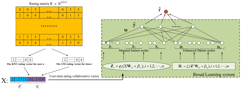
Figure 1: Illustration of the proposed BroadCF algorithm.

III-B Preliminaries

BLS is a lightweight neural network that can approximate any function [32], which has been widely used in many different applications [49, 50, 51, 52, 53, 54]. It is derived from the Random Vector Functional Linked Neural Network (RVFLNN) [55]. In BLS, the original data are firstly mapped into the mapped features by random weights, which are stored in the mapped feature nodes. Next, the mapped features are further mapped by random weights to obtain the enhanced features, which are used for extensive scaling. Finally, the parameter normalization optimization is solved using the ridge regression approximation to learn the final network weights.

The advantage of BLS is that it can use random hidden layer weights to map the original data points to a discriminative feature space tensed by these vectors. In the hidden layer, the parameters are randomly generated in accordance with any continuous probability distribution, the rationale of which has been theoretically proven. This random mechanism provides a fast training process for BLS. It solves the serious training time consuming problem suffered by the DNNs-based models. Specifically, BLS can be updated incrementally when adding newly samples and hidden nodes, without the need of rebuilding the entire network from scratch. As a result, BLS requires a small amount of parameters to be stored, which can solve the problem of huge storage requirements arising from the DNNs-based models. Most importantly, in BLS, the feature layer is directly connected to the output layer, and the structure is very simple but effective. Therefore, even without a large amount of samples in RSs, the prediction performance can be ensured.

IV Broad Collaborative Filtering

In this section, we will describe the proposed Broad Collaborative Filtering (BroadCF) method in detail. First of all, we will describe how to transform the original user-item rating data into the form of (Rating collaborative vector, Rating) for every user-item pair, which will be taken as input and output to BLS respectively. Then, we will describe the broad learning part. Finally, we will describe the rating prediction procedure and summarize the propose BroadCF method. For clarity purpose, Figure 1 illustrates the major procedure of the BroadCF method.

IV-A Data Preprocessing

From Eq. (2), for each user-item pair $(u,v)$, the model-based RSs aim to establish a mapping function from the user-item input data to the user-item rating. A simple type of user-item input data is the direct concatenation of the rating vectors ${\mathbf{R}}_{u,:}$ and ${\mathbf{R}}_{:,v}$ of user $u$ and item $v$ respectively. It has been commonly adopted in the DNNs-based methods, i.e., the DNNs-based methods learn the latent factor vectors from the original user/item rating vectors. However, it does not work well in the case of BLS, as will be explained below. The DNNs-based methods stack several hidden layers with decreasing layer sizes, e.g., from the $10^{4}$-dimensional input to the first hidden layer of $10^{3}$ dimension, and further to the second hidden layer of $10^{2}$ dimension, etc. On the contrary, as will be shown later, BLS requires broadening the original input features into the mapped features and the enhanced features, e.g., from the $10^{4}$-dimensional input to the mapped features of $10^{5}$ dimension, and further to the enhanced features of $10^{6}$ dimension, resulting in several-order magnitude larger dimension. In addition, directly utilizing extremely sparse user rating vector and item rating vector may cause the overfitting issue. Inspired by the previous work [29], a new preprocessing procedure is designed to generate user-item rating collaborative vector, which is a low-dimensional user-item input vector that can leverage quality judgments of the most similar users/items.

IV-A1 KNU Rating Vector

First of all, for each user $u$, a set of $k$ nearest users (KNU) is searched by computing the cosine similarity between the rating vector of the target user $u$ and those of the other users. And their indexes are stored in the KNU index vector $\bm{\pi}^{u}\in\mathbb{R}^{1\times k}$, i.e., the $i$-th nearest user of the target user $u$ can be expressed as $\bm{\pi}^{u}[i],\forall i=1,\cdots,k$. Based on the KNU index vector $\bm{\pi}^{u}$ and the rating matrix $\mathbf{R}$, for the user-item pair $(u,v)$, we can obtain the KNU rating vector ${\mathbf{p}}_{v}^{u}\in\mathbb{R}^{1\times k}$ of user $u$ on item $v$ with each entry ${\mathbf{p}}_{v}^{u}[i]$ being defined as follows,

$$\begin{aligned} \mathbf{p}_{v}^{u}[i]=\mathbf{R}_{\bm{\pi}^{u}[i],v}~{}~{}~{}\forall i=1,\cdots,{k}.\end{aligned}$$ (3)

That is, ${\mathbf{p}}_{v}^{u}[i]$ is the rating value of user $\bm{\pi}^{u}[i]$ to item $v$.

In the above procedure, it is possible that some entries ${\mathbf{p}}_{v}^{u}[i]$ are zeros, i.e., user $\bm{\pi}^{u}[i]$ did not rate item $v$. In [29], the mean value of the ratings of user $\bm{\pi}^{u}[i]$ is used to fill the missing rating, which however, treats all the unrated items of user $\bm{\pi}^{u}[i]$ equally while failing to utilize the rating of other similar users to item $v$. To this end, a more reasonable strategy is designed as follows,

$$\begin{aligned} &\mathbf{\bar{p}}_{v}^{u}[i]=\\ &\begin{cases}\mathbf{p}_{v}^{u}[i]&\text{~{}~{}~{}if~{}}\mathbf{p}_{v}^{u}[i]\neq 0\\ \mathbf{R}_{u^{*},v}&\text{~{}~{}~{}if~{}}\mathbf{p}_{v}^{u}[i]=0\&\text{sim}(u^{*},\bm{\pi}^{u}[i])\geq\theta\\ \text{mean}(\mathbf{R}_{{\bm{\pi}^{u}[i]},:})&\text{~{}~{}~{}if~{}}\mathbf{p}_{v}^{u}[i]=0\&\text{sim}(u^{*},\bm{\pi}^{u}[i])<\theta\end{cases}\end{aligned}$$ (4)

where $u^{*}$ denotes the nearest user of user $\bm{\pi}^{u}[i]$ who has rated item $v$, $\text{sim}(u^{*},\bm{\pi}^{u}[i])\geq\theta$ indicates that the similarity between user $u^{*}$ and user $\bm{\pi}^{u}[i]$ is no smaller than the threshold $\theta$, and $\text{mean}(\mathbf{R}_{{\bm{\pi}^{u}[i]},:})$ denotes the mean value of the ratings of user $\bm{\pi}^{u}[i]$. That is, when user $\bm{\pi}^{u}[i]$ did not rate item $v$ (i.e. $\mathbf{p}_{v}^{u}[i]=0$), we first search the most similar user of user $\bm{\pi}^{u}[i]$ who has already rated item $v$, denoted as user $u^{*}$. If the similarity between user $u^{*}$ and user $\bm{\pi}^{u}[i]$ is no smaller than the threshold $\theta$, we use the rating of user $u^{*}$ on item $v$ to fill the missing rating of user $\bm{\pi}^{u}[i]$ on item $v$. Otherwise, we use the mean value of the ratings of user $\bm{\pi}^{u}[i]$ to fill the missing rating of user $\bm{\pi}^{u}[i]$ on item $v$.

IV-A2 LNI Rating Vector

Similarly, for each item $v$, a set of $l$ nearest items (LNI) is searched by computing the cosine similarity between the rating vectors of the target item $v$ and the other items. And their indexes are stored in the LNI index vector $\bm{\eta}^{v}\in\mathbb{R}^{1\times l}$, i.e., the $i$-th nearest item of item $v$ can be expressed as $\bm{\eta}^{v}[i],\forall i=1,\cdots,l$. Based on the LNI index vector $\bm{\eta}^{v}$ and the rating matrix $\mathbf{R}$, for the user-item pair $(u,v)$, we can obtain the LNI rating vector $\mathbf{q}_{v}^{u}\in\mathbb{R}^{1\times l}$ of user $u$ on item $v$ with each entry $\mathbf{q}_{v}^{u}[i]$ being defined as follows,

$$\begin{aligned} \mathbf{q}_{v}^{u}[i]=\mathbf{R}_{u,\bm{\eta}^{v}[i]}~{}~{}~{}\forall i=1,\cdots,l.\end{aligned}$$ (5)

That is, $\mathbf{q}_{v}^{u}[i]$ denotes the rating value of user $u$ to item $\bm{\eta}^{v}[i]$.

Like before, the following strategy is used to fill the missing entries

$$\begin{aligned} &\mathbf{\bar{q}}_{v}^{u}[i]=\\ &\begin{cases}\mathbf{q}_{v}^{u}[i]&\text{~{}~{}~{}if~{}}\mathbf{q}_{v}^{u}[i]\neq 0\\ \mathbf{R}_{u,v^{*}}&\text{~{}~{}~{}if~{}}\mathbf{q}_{v}^{u}[i]=0\&\text{sim}(v^{*},\bm{\eta}^{v}[i])\geq\theta\\ \text{mean}(\mathbf{R}_{:,\bm{\eta}^{v}[i]})&\text{~{}~{}~{}if~{}}\mathbf{q}_{v}^{u}[i]=0\&\text{sim}(v^{*},\bm{\eta}^{v}[i])<\theta\end{cases}\end{aligned}$$ (6)

where $v^{*}$ denotes the nearest item of item $\bm{\eta}^{v}[i]$ rated by user $u$, $\text{sim}(v^{*},\bm{\eta}^{v}[i])\geq\theta$ indicates that the similarity between item $v^{*}$ and item $\bm{\eta}^{v}[i]$ is no smaller than the threshold $\theta$, and $\text{mean}(\mathbf{R}_{:,\bm{\eta}^{v}[i]})$ denotes the mean value of the ratings of item $\bm{\eta}^{v}[i]$.

IV-A3 User-Item Rating Collaborative Vector

After obtaining $\bar{\mathbf{p}}_{v}^{u}$ and $\bar{\mathbf{q}}_{v}^{u}$, a user-item rating collaborative vector is obtained by concatenation, i.e.,

$$\mathbf{x}_{v}^{u}=\left[\bar{\mathbf{p}}_{v}^{u}|\bar{\mathbf{q}}_{v}^{u}\right]\in\mathbb{R}^{1\times(k+l)}.$$ (7)

Note that the dimension of the input data $\mathbf{x}_{v}^{u}$, i.e. $k+l$, is much smaller than that of the direct concatenation of the rating vectors $\mathbf{R}_{u,:}$ and $\mathbf{R}_{:,v}$ of user $u$ and item $v$, i.e. $|\mathcal{V}|+|\mathcal{U}|$.

IV-A4 Training Data of BLS

Finally, for every user-item pair $(u,v)$ with known rating in the training rating matrix, the user-item rating collaborative vector $\mathbf{x}_{v}^{u}$ and the user-item rating $r_{u,v}$ are taken as the input and output of a training sample $(\mathbf{x}_{v}^{u},r_{u,v})$ respectively. That is, the training set of the proposed BroadCF method is

$$\mathcal{D}=\{(\mathbf{x}_{v}^{u},r_{u,v})|\mathbf{R}_{u,v}\neq 0\}.$$ (8)

IV-B Broad Learning

In this subsection, we will describe the mapping function $f$ that maps the rating collaborative vector $\mathbf{x}_{v}^{u}$ into the predicted rating $r_{u,v}$, which will be achieved by BLS. According to [32], BLS is composed of three modules, namely mapped feature layer, enhanced feature layer, and output layer.

IV-B1 Mapped Feature Layer

Given the training set $\mathcal{D}=\{(\mathbf{x}_{v}^{u},r_{u,v})|\mathbf{R}_{u,v}\neq 0\}$, the training input matrix of BLS is formed as

$$\mathbf{X}=\left[\begin{array}[]{c}\mathbf{x}_{v_{1}}^{u_{1}}\\ \mathbf{x}_{v_{2}}^{u_{2}}\\ \vdots\\ \mathbf{x}_{v_{|\mathcal{D}|}}^{u_{|\mathcal{D}|}}\\ \end{array}\right]\in\mathbb{R}^{|\mathcal{D}|\times(k+l)}$$ (9)

where $|\mathcal{D}|$ is the training sample number, i.e., there are $|\mathcal{D}|$ user-item pairs $(u_{1},v_{1}),(u_{2},v_{2}),...,(u_{|\mathcal{D}|},v_{|\mathcal{D}|})$. The training output vector of BLS is formed as

$$\mathbf{y}=\left[\begin{array}[]{c}r_{u_{1},v_{1}}\\ r_{u_{2},v_{2}}\\ \vdots\\ r_{u_{|\mathcal{D}|},v_{|\mathcal{D}|}}\\ \end{array}\right]\in\mathbb{R}^{|\mathcal{D}|\times 1}.$$ (10)

In the mapped feature layer, the input matrix $\mathbf{X}$ is transformed into the mapped feature matrix $\mathbf{Z}_{i}\in\mathbb{R}^{|\mathcal{D}|\times d_{z}}$ as follows

$$\begin{aligned} \mathbf{Z}_{i}=\phi_{i}(\mathbf{X}\mathbf{W}_{z_{i}}+\bm{\beta}_{z_{i}}),~{}~{}i=1,2,\cdots,n\end{aligned}$$ (11)

where $d_{z}$ denotes the dimension of each mapped feature group, $n$ is the number of the mapped feature groups, and $\phi_{i}$ is the $i$-th nonlinear feature mapping function. In our experiments, ReLu is used as the nonlinear feature mapping function. In the above procedure, $\mathbf{W}_{z_{i}}\in\mathbb{R}^{(k+l)\times d_{z}}$ and $\bm{\beta}_{z_{i}}\in\mathbb{R}^{|\mathcal{D}|\times d_{z}}$ are randomly generated matrices. In this way, the mapped feature matrices can be obtained, i.e.,

$$\mathbf{Z}^{n}=[\mathbf{Z}_{1}|\mathbf{Z}_{2}\cdots|\mathbf{Z}_{n}]\in\mathbb{R}^{|\mathcal{D}|\times nd_{z}}.$$ (12)

Algorithm 1 Broad Collaborative Filtering (BroadCF)

Training part:

1:Input: $\mathbf{R}$: training rating matrix; $k$: number of the nearest users; $l$: number of the nearest items; $n$: number of mapped feature groups; $d_{z}$: mapped feature dimension; $m$: number of enhanced feature groups; $d_{h}$: enhanced feature dimension.

2:Search the $k$ nearest users of each user $u$.

3:Search the $l$ nearest items of each item $v$.

4:for all training user-item pair with $\mathbf{R}_{u,v}\neq 0$ do

5:   Generate user-item rating collaborative vector $\mathbf{x}^{u}_{v}$ via Eq. (7).

6:end for

7:Generate the training set $\mathcal{D}$ via Eq. (8).

8:Generate the training input matrix $\mathbf{X}$ and training output vector $\mathbf{y}$ via Eq. (9) and Eq. (10) respectively.

9:Generate the mapped feature matrices $\mathbf{Z}^{n}$ and enhanced feature matrices $\mathbf{H}^{m}$ via Eq. (12) and Eq. (14) respectively.

10:Calculate the trainable weight vector $\mathbf{w}$ via Eq. (16).

11:Output: The trainable weight vector $\mathbf{w}$.

Testing part:

1:Input: A user-item pair $(u,v)$ with unknown rating.

2:Generate user-item rating collaborative vector $\mathbf{x}^{u}_{v}$ via Eq. (7).

3:Feed $\mathbf{x}^{u}_{v}$ into the broad learning procedure to generate the predicted user-item rating $\hat{r}^{u}_{v}$.

4:Output: The predicted rating $\hat{r}^{u}_{v}$.

IV-B2 Enhanced Feature Layer

After obtaining $\mathbf{Z}^{n}$, the enhanced feature matrix $\mathbf{H}_{i}\in\mathbb{R}^{|\mathcal{D}|\times d_{h}}$ is calculated as follows,

$$\begin{aligned} \mathbf{H}_{i}=\xi_{i}(\mathbf{Z}^{n}\mathbf{W}_{h_{i}}+\bm{\beta}_{h_{i}}),~{}~{}i=1,2,\cdots,m\end{aligned}$$ (13)

where $d_{h}$ denotes the dimension of each enhanced feature group, $m$ is the number of the enhanced feature groups, and $\xi_{i}$ is the $i$-th nonlinear feature enhancement function. In our experiments, ReLu is used as the nonlinear feature enhancement function. In the above procedure, $\mathbf{W}_{h_{i}}\in\mathbb{R}^{nd_{z}\times d_{h}}$ and $\bm{\beta}_{h_{i}}\in\mathbb{R}^{|\mathcal{D}|\times d_{h}}$ are randomly generated matrices. In this way, the enhanced feature matrices is obtained, i.e.,

$$\mathbf{H}^{m}=[\mathbf{H}_{1}|\mathbf{H}_{2}\cdots|\mathbf{H}_{m}]\in\mathbb{R}^{|\mathcal{D}|\times md_{h}}.$$ (14)

IV-B3 Output Layer

After obtaining the mapped feature matrices $\mathbf{Z}^{n}$ and the enhanced feature matrices $\mathbf{H}^{m}$, the output vector $\mathbf{y}\in\mathbb{R}^{|\mathcal{D}|\times 1}$ can be predicted as

$$\begin{aligned} \begin{aligned} \mathbf{y}&=\left[\mathbf{Z}^{n}|\mathbf{H}^{m}\right]\mathbf{w}\end{aligned}\end{aligned}$$ (15)

where $\mathbf{w}\in\mathbb{R}^{(nd_{z}+md_{h})\times 1}$ is the trainable weight vector that maps the concatenated mapped and enhanced features into the output $\mathbf{y}$.

In the training procedure, the only trainable weight vector $\mathbf{w}$ can be solved by applying the ridge regression approximation of pseudoinverse $\left[\mathbf{Z}^{n}|\mathbf{H}^{m}\right]^{+}$, i.e.,

$$\mathbf{w}=\left[\mathbf{Z}^{n}|\mathbf{H}^{m}\right]^{+}\mathbf{y}.$$ (16)

IV-C Rating Prediction and Algorithm Summary

In the testing procedure, for every user-item pair $(u,v)$ with unknown rating, the predicted rating can be obtained by feeding the user-item rating collaborative vector $\mathbf{x}_{v}^{u}\in\mathbb{R}^{1\times(k+l)}$ into the broad learning procedure, which outputs the predicted user-item rating $\hat{r}_{u,v}$. For clarity, Algorithm 1 summarizes the main procedure of BroadCF.

TABLE II: Statistic information of the seven datasets.

Datasets	#Users	#Items	#Ratings	Sparsity	Scale
ml-la	610	9,724	100,836	98.30%	[1, 5]
Amazon-DM	1000	4,796	11,677	99.90%	[1, 5]
Amazon-GGF	2,500	7,527	11,532	99.96%	[1, 5]
Amazon-PLG	5,000	5,400	12,429	99.98%	[1, 5]
Amazon-Automotive	5,000	6,596	12,665	99.98%	[1, 5]
Amazon-Baby	6,000	5,428	17,532	99.98%	[1, 5]
Amazon-IV	429,622	23,966	583,933	99.98%	[1, 5]

TABLE III: The comparison results on prediction performance: The mean value and standard deviation (std. dev.) of RMSE achieved by running each algorithm five times on each dataset.

Methods	ml-la		Amazon-DM		Amazon-GGF		Amazon-PLG		Amazon-Automotive		Amazon-Baby		Amazon-IV
	Mean	Std. dev.	Mean	Std. dev.	Mean	Std. dev.	Mean	Std. dev.	Mean	Std. dev.	Mean	Std. dev.	Mean	Std. dev.
PMF	1.0016	0.0029	2.2170	0.0122	3.2144	0.0263	3.0658	0.0346	3.2621	0.0329	2.6281	0.0225	NA	NA
NeuMF	2.3643	0.0042	2.0587	0.0253	2.3508	0.0497	1.7665	0.0391	2.9946	0.0310	2.9796	0.0374	1.2749	0.0258
DMF	1.6325	0.0034	3.6161	0.0215	4.1642	0.0328	4.1030	0.0216	4.1488	0.1088	3.2546	0.0154	NA	NA
DeepCF	2.1133	0.0094	1.7025	0.0217	1.2487	0.0314	1.6426	0.0452	1.6352	0.0449	1.6669	0.0441	NA	NA
BPAM	0.8484	0.0035	1.2509	0.0132	1.7281	0.0274	1.9805	0.0328	1.9805	0.0373	0.8678	0.0301	2.4521	0.0324
SHT	1.5023	0.0096	2.2758	0.1082	1.9724	0.0501	1.6721	0.1120	1.4503	0.0731	2.0094	0.0636	NA	NA
BroadCF	0.7220	0.0363	0.7292	0.1542	0.9683	0.1110	0.9877	0.0698	0.8570	0.0155	0.8528	0.0426	0.7933	0.0542

TABLE IV: The comparison results on prediction performance: The mean value and standard deviation (std. dev.) of MAE achieved by running each algorithm five times on each dataset.

Methods	ml-la		Amazon-DM		Amazon-GGF		Amazon-PLG		Amazon-Automotive		Amazon-Baby		Amazon-IV
	Mean	Std. dev.	Mean	Std. dev.	Mean	Std. dev.	Mean	Std. dev.	Mean	Std. dev.	Mean	Std. dev.	Mean	Std. dev.
PMF	0.7525	0.0026	1.6670	0.0107	2.9038	0.0320	2.6038	0.0281	2.8330	0.0269	2.1097	0.0117	NA	NA
NeuMF	1.9791	0.0032	1.3896	0.0221	1.6070	0.0374	1.7446	0.0323	2.5148	0.0215	2.4489	0.0308	1.0138	0.0211
DMF	1.2297	0.0037	3.4477	0.0275	3.9433	0.0305	3.8417	0.0226	3.9055	0.1004	3.2546	0.0131	NA	NA
DeepCF	1.6345	0.0082	1.6202	0.0188	1.2237	0.0296	1.6189	0.0360	1.6798	0.0391	1.5738	0.0319	NA	NA
BPAM	0.6570	0.0024	1.5800	0.0175	1.2425	0.0212	1.5440	0.0290	0.6790	0.0326	1.4900	0.0257	1.9529	0.0289
SHT	1.4391	0.0105	1.7279	0.0658	1.5720	0.0419	1.4839	0.0914	1.2942	0.0739	1.4900	0.0541	NA	NA
BroadCF	0.5353	0.0274	0.5151	0.1320	0.5903	0.0563	0.6512	0.0698	0.5202	0.0585	0.5672	0.0432	0.3994	0.0507

V Experiments

In this section, extensive experiments will be conducted to confirm the effectiveness of the proposed BroadCF method. All experiments are conducted in Python and run on a server with an Intel Core i9-10900 CPU, GeForce RTX 3090, and 256GB of RAM.

V-A Experimental Settings

V-A1 Datasets

In our experiments, seven real-world publicly available datasets are used, which are obtained from the two main sources.

1. MovieLens: The MovieLens dataset contains rating data of movies by users. For experimental purpose, we use the ml-latest dataset (abbr. ml-la).

2. Amazon: It is an upgraded version of the Amazon review dataset for 2018 [56], which contains reviews (ratings, text, and helpful polls), product meta-data (category information, brand and image features, price, and descriptions) and links (also view/buy charts). For experimental purpose, we use six datasets, namely Digital-Music (Amazon-DM), Grocery-and-Gourmet-Food (Amazon-GGF), Patio-Lawn-and-Garden (Amazon-PLG), Automotive (Amazon-Automotive), Baby (Amazon-Baby), and Instant-Video (Amazon-IV).

Table II summarizes the statistic information of the above seven datasets. From the table, we can see that Amazon-IV is relatively very large. On each dataset, the rating information of each user is randomly split into the training set (75%) and the testing set (25%). Furthermore, in the training set, a quarter of the ratings are randomly selected as the validation set to tune the hyper-parameters for all the methods.

V-A2 Evaluation Measures

To evaluate the performance of rating prediction, two evaluation measures are used, namely Root Mean Square Error (abbr. RMSE) and Mean Absolute Error (abbr. MAE). The two measures are calculated via computing the rating prediction error w.r.t. the ground-truth rating, where smaller values indicate better rating prediction results. In addition, the running cost, including training time, testing time, and trainable parameter storage cost is also used as evaluation criteria.

V-B Comparison Results

V-B1 Baselines

The proposed BroadCF approach is compared with the following six approaches.

• PMF [39] is a classical CF approach that considers only latent factors and uses matrix decomposition to capture the linear relationships in the user-item pairs.

• NeuMF [27] takes as input the connection of user/item embeddings and uses the MLP model for prediction.

• DMF [26] uses a dual-path neural network instead of the linear embedding operation used in the conventional matrix decomposition.

• DeepCF [31] integrates a unified deep collaborative filtering framework with representation learning and matching function learning.

• BPAM [29] is a neighborhood-based CF recommendation framework that captures the global influence of a target user’s nearest users on their nearest target set of users by introducing a global attention matrix.

• SHT [47] introduces the hypergraph transformer network for collaborative filtering recommendation via self-supervised learning.

The hyper-parameters of the above six methods are tuned as suggested by the original authors. In PMF, the factor number is set to 30 for both users and items, and the regularization hyper-parameters are set to 0.001 and 0.0001 for users and items respectively. In NeuMF, the number of predictors for the generalized matrix decomposition part and the embedding sizes for users and items are set as 8 and 16, respectively. In DMF, the predictor number is set to 64 for both users and items. In DeepCF, the sizes of the MLP layers and the DMF layers in the representation learning and the matching function learning are both set to [512, 256, 128, 64]. In BPAM, the numbers of the nearest users and items are tuned in [3, 5, 7, 9]. In SHT, the number of GNN layers and the learning rate are set to 2 and 0.001 respectively. For the deep models, i.e., NeuMF, DMF, DeepCF and SHT, the batch size is set as 256. In BroadCF, we set the number of both nearest users and nearest items as 5, i.e., $k=l=5$, the number of both mapped feature groups and enhanced feature groups as 7, i.e., $n=m=7$, and the mapped feature dimension and the enhanced feature dimension as 3, i.e., $d_{z}=d_{h}=3$. For the DNNs-based methods, including NeuMF, DMF, DeepCF and SHT, GPUs are used, while for the rest methods, including PMF, BPAM and BroadCF, GPU is not used. The code of BroadCF is made publicly available at https://github.com/BroadRS/BroadCF.

TABLE V: The comparison results on running cost: The training time (in seconds) consumed by each algorithm on each dataset.

Methods	ml-la	Amazon-DM	Amazon-GGF	Amazon-PLG	Amazon-Automotive	Amazon-Baby	Amazon-IV
PMF	98.24	202.92	1132.87	4072.20	4311.29	1100.17	NA
NeuMF	6013.53	109.42	75.38	68.71	80.47	101.84	48219.60
DMF	2462.42	62.70	85.75	123.25	104.01	209.50	NA
DeepCF	2059.59	202.80	306.60	362.40	366.40	501.00	NA
BPAM	159.36	128.72	143.30	125.70	130.27	137.80	11416.20
SHT	48.67	26.05	42.14	61.78	64.33	71.03	NA
BroadCF	38.00	2.60	2.49	3.37	5.08	7.06	14.57

TABLE VI: The comparison results on running cost: The testing time (in seconds) consumed by each algorithm on each dataset.

Methods	ml-la	Amazon-DM	Amazon-GGF	Amazon-PLG	Amazon-Automotive	Amazon-Baby	Amazon-IV
PMF	0.03	0.01	0.01	0.01	0.01	0.01	NA
NeuMF	301.40	118.53	189.72	331.24	464.19	450.14	10825.30
DMF	21.11	7.95	29.69	95.61	73.82	126.90	NA
DeepCF	427.09	67.44	102.65	120.89	94.47	171.50	NA
BPAM	0.76	0.11	0.13	0.20	0.19	0.28	7.13
SHT	2.32	0.09	0.17	0.27	0.32	0.35	NA
BroadCF	1.18	0.08	0.08	0.10	0.14	0.19	6.55

TABLE VII: The comparison results on running cost: The number of trainable parameters to be stored during the training procedure of each algorithm on each dataset.

	ml-la	Amazon-DM	Amazon-GGF	Amazon-PLG	Amazon-Automotive	Amazon-Baby	Amazon-IV
PMF	310,080	173,910	300,840	312,030	347,910	342,900	NA
NeuMF	392,601	234,521	403,761	418,681	466,521	459,801	18,038,161
DMF	12,327,168	33,519,232	40,030,464	48,012,672	20,921,728	29,942,272	NA
DeepCF	39,266,060	97,444,766	115,947,300	137,582,762	62,738,578	86,977,048	NA
BPAM	43,615	31,500	78,750	157,500	157,500	189,000	7,518,367
SHT	509,025	363,777	511,105	499,169	549,377	544,001	NA
BroadCF	3,125	3,125	3,125	3,125	3,125	3,125	3,125

V-B2 Comparison on Prediction Performance

The comparison results on the prediction performance measured by RMSE and MAE are listed in Table III and Table IV respectively. In the comparison experiment, each method is run 5 times on each dataset, and the mean value and standard deviation (std. dev.) over the 5 runs are listed. Out-of-memory errors occur when training PMF, DMF, DeepCF and SHT on the largest Amazon-IV dataset. This is because the four models take the user-item rating matrix as input, but for the Amazon-IV dataset, the entire rating matrix takes up to $32\cdot|\mathcal{U}|\cdot|\mathcal{V}|$ bits of memory, which is about 308.64 GB, exceeding 256 GB memory of the experimental machine. As a result, no result is reported in the corresponding entries of the comparison result tables (i.e. NA). From the two tables, we have the following observations.

Overall, the values of RMSE and MAE achieved by the proposed BroadCF algorithm are much smaller than those by the other algorithms, including the classical CF method (PMF), four DNNs-based algorithms (DMF, NeuMF, DeepCF and SHT), and one BP neural network-based method (BPAM). In particular, compared with PMF, the proposed BroadCF algorithm achieves at least 27.91% and 28.86% improvements of RMSE and MAE, which is a relatively significant performance improvement. The main reason is that PMF only captures the linear latent factors, i.e. the linear relationships in the user-item pairs, while BroadCF is able to capture the nonlinear relationships in the user-item pairs. Compared with the four DNNs-based algorithms, BroadCF also obtains significant improvements of RMSE and MAE, which is a more significant performance improvement. The main reason may be that, although both the DNNs-based algorithms and BroadCF are able to capture the nonlinear relationships in the user-item pairs, the DNNs-based algorithms easily encounter the overfitting issue, i.e., given the very large number of trainable parameters, the testing performance cannot be improved compared with the training performance. As a contrast, compared with BPAM, which is a lightweight neural network based method, the prediction performance of BroadCF is still better than that of BPAM, although the performance improvement is not such significant. As will be shown in the comparison on running cost, the number of trainable parameters in BPAM is relatively small compared with those of the DNNs-based algorithms, although still larger than that of BroadCF. Overall, the comparison results on the prediction performance have demonstrated the effectiveness of the proposed BroadCF method.

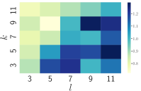
(a) ml+la

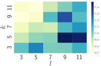
(b) Amazon-DM

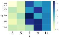
(c) Amazon-GGF

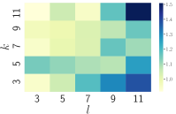
(d) Amazon-PLG

Figure 2: Hyper-parameter analysis: The results in terms of RMSE achieved by BroadCF with different ${k}$ and $l$.

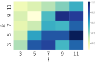
(a) ml-la

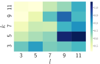
(b) Amazon-DM

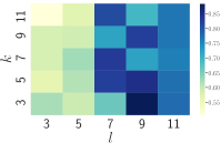
(c) Amazon-GGF

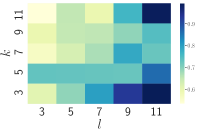
(d) Amazon-PLG

Figure 3: Hyper-parameter analysis: The results in terms of MAE achieved by BroadCF with different ${k}$ and $l$.

V-B3 Comparison on Running Cost

Apart from the prediction and recommendation performance, BroadCF has superiority on running cost. To this end, this subsection compares the running cost of BroadCF with the baselines, including the training time, testing time, and trainable parameter storage cost.

(a) ml-la

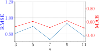
(b) Amazon-DM

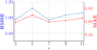
(c) Amazon-GGF

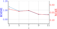
(d) Amazon-PLG

Figure 4: Hyper-parameter analysis: The results in terms of RMSE and MAE achieved by BroadCF with different $n$.

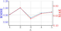
(a) ml-la

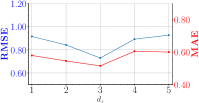
(b) Amazon-DM

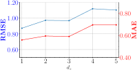
(c) Amazon-GGF

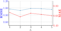
(d) Amazon-PLG

Figure 5: Hyper-parameter analysis: The results in terms of RMSE and MAE achieved by BroadCF with different $d_{z}$.

Table V and Table VI report the training time and the testing time (in seconds) consumed by each algorithm on each dataset. Specifically, the training time and the testing time account for the time from feeding the preprocessed data into the model to outputting the results. According to the two tables, we can see that the proposed BroadCF algorithm is very efficient on running time. In particular, from Table V, BroadCF consumes several-magnitude shorter running time compared with the baselines. On the ml-la dataset, BroadCF is twice faster than the fastest baseline namely PMF, and it consumes about 23% running time by BPAM. Most importantly, when comparing with the DNNs-based models except SHT, BroadCF consumes less than 2% running time on ml-la, while BroadCF is still slightly faster than SHT. On the six Amazon datasets, the five neural network based baselines namely NeuMF, DMF, DeepCF, BPAM and SHT, are faster than PMF. This is mainly due to that the neural network models take the rating vectors, which is relatively efficient in the case of relatively sparse dataset with small number of ratings. However, BroadCF is still much faster than the five neural network based baselines. This may be due to that the optimization problem of BroadCF is solved by using the ridge regression approximation of pseudoinverse without need of iterative training process.

From Table VI, we can see that although BroadCF is not the fastest algorithm on the testing time, it is very close to the fastest baseline namely PMF. This is mainly due to that, BroadCF requires calculating the mapped features and enhanced features, in addition to the multiplication by the trainable weight vector, while PMF only requires to compute the matching score of the user/item latent factors. Nevertheless, BroadCF is still much faster than the five neural network based baselines namely NeuMF, DMF, DeepCF, BPAM and SHT. The above comparison results on training time and testing time have demonstrated the efficiency of the proposed BroadCF method from the perspective of running time.

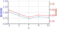
(a) ml-la

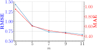
(b) Amazon-DM

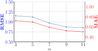
(c) Amazon-GGF

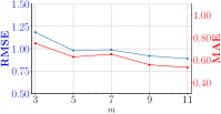
(d) Amazon-PLG

Figure 6: Hyper-parameter analysis: The results in terms of RMSE and MAE achieved by BroadCF with different $m$.

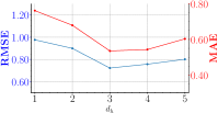
(a) ml-la

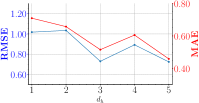
(b) Amazon-DM

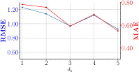
(c) Amazon-GGF

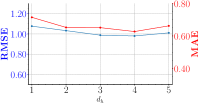
(d) Amazon-PLG

Figure 7: Hyper-parameter analysis: The results in terms of RMSE and MAE achieved by BroadCF with different $d_{h}$.

We also demonstrate the efficiency of BroadCF from the perspective of storage requirements. Following [29], Table VII reports the number of trainable parameters to be stored during the training procedure of each algorithm on each dataset. From the table, we can see that, the proposed BroadCF algorithm is several-magnitude more efficient than all the baselines. This is mainly due to that the only trainable parameters to be stored in BroadCF are the weight vector $\mathbf{w}\in\mathbb{R}^{(nd_{z}+md_{h})\times 1}$, which is independent of the input data size and dimension. On the contrary, all the baselines need to store much more trainable parameters, especially for the DNNs-based models. This result also confirms the fact that BroadCF requires several-magnitude less training parameters, even less than the linear model namely PMF. Despite the relatively small number of trainable parameters, BroadCF can still well capture the nonlinear relationships in the user-item pairs and therefore generates much better results as shown in the comparison of prediction and recommendation performance. This is mainly due to the advantage achieved by mapping the original features into the mapped features and then into the enhanced features via random matrices plus nonlinear activation functions, which can be regarded as learning nonlinear representations from different views. Overall, the above comparison results on running cost have confirmed the efficiency of the proposed BroadCF algorithm from the perspective of trainable parameter storage requirement.

V-C Hyper-Parameter Analysis

In this subsection, we will analyze the effect of six hyper-parameters on the prediction performance of BroadCF, i.e., nearest user number $k$, nearest item number $l$, number of mapped feature groups $n$, mapped feature dimension $d_{z}$, number of enhanced feature groups $m$, and enhanced feature dimension $d_{h}$. When investigating one hyper-parameter, the other hyper-parameters are fixed. Due to the space limit, only the first four datasets are analyzed in this part of experiments, i.e., ml-la, Amazon-DM, Amazon-GGF and Amazon-PLG. Notice that the three Amazon datasets cover different degrees of sparsity, namely 99.90%, 99.96% and 99.98%. And similar observations can be obtained on the remaining datasets.

V-C1 Number of the Nearest Users/Items

First of all, we will investigate the effect of the number of the nearest users/items, namely $k$ and $l$, on the prediction performance of BroadCF. To this end, we run BroadCF by setting $k$ and $l$ in the range of [3, 5, 7, 9, 11], and report the prediction performance measured by RMSE and MAE in Figure 2 and Figure 3 respectively. From the figures, we can observe that a relatively stable performance is achieved when using different $k$ and $l$ on most datasets. That is, the variances of the RMSE and MAE values in the two figures are relatively small as shown in the heatmaps. However, a general trend is that when increasing $k$ and $l$, the prediction performance would slightly degenerate expect on the ml-la dataset. This is mainly due to the long-tail distribution, i.e., most of users/items have very few ratings. Setting a relatively large number of the nearest users/items would mistakenly introduce more noises, i.e., filling the missing entries by means of the nearest rating via Eq. (4) and Eq. (6). And the exception on the ml-la dataset has confirmed this analysis. That is, ml-la is a relatively dense dataset compared with the other datasets, in which the users/items contain more ratings. Regarding the trade-off between the running efficiency and the accuracy, we set $k$ and $l$ to 5 in the experiments.

V-C2 Hyper-Parameters in Feature Mapping

Secondly, we will investigate the effect of the hyper-parameters in the feature mapping module, including the number of mapped feature groups $n$ and the mapped feature dimension $d_{z}$. In the proposed BroadCF algorithm, the feature mapping module plays the role of mapping the original input matrix composed of user-item collaborative vectors into the mapped feature matrix, which is the first step of capturing the nonlinear relationships in the user-item pairs. The two hyper-parameters would affect the performance of this mapping capability. To this end, we run BroadCF by setting $n$ and $d_{z}$ in the ranges of [3,5,7,9,11] and [1,2,3,4,5] respectively, and report the RMSE and MAE values as a function of $n$ and $d_{z}$ in Figure 4 and Figure 5 respectively. From the two figures, although the best values of $n$ and $d_{z}$ differ on different datasets, the performance variation is relatively small. This confirms the relatively insensitivity of the proposed BroadCF algorithm to the hyper-parameters in feature mapping. And in our experiments, we set $n$ and $d_{z}$ to 7 and 3 respectively.

V-C3 Hyper-Parameters in Feature Enhancement

Similar to the previous subsection, we will also investigate the effect of the hyper-parameters in feature enhancement module, including the number of enhanced feature groups $m$ and the enhanced feature dimension $d_{h}$. In the proposed BroadCF algorithm, the feature enhancement module plays the role of mapping the mapped feature matrices into the enhanced feature matrix, which is the second step of capturing the nonlinear relationships in the user-item pairs. The two hyper-parameters would affect the prediction performance of this enhancement capability. Similarly, we run BroadCF by setting $m$ and $d_{h}$ in the ranges of [3,5,7,9,11] and [1,2,3,4,5] respectively, and report the RMSE and MAE values as a function of $m$ and $d_{h}$ in Figure 6 and Figure 7 respectively. From the two figures, although the best values of $m$ and $d_{h}$ differ on different datasets, the performance variation is relatively small. This confirms the relatively insensitivity of the proposed BroadCF algorithm to the hyper-parameters in feature enhancement. And in our experiments, we set $m$ and $d_{h}$ to 7 and 3 respectively.

VI Conclusions

In this paper, we have developed a novel neural network based recommendation method called Broad Collaborative Filtering (BroadCF). Compared with the existing DNNs-based recommendation methods, the proposed BroadCF method is also able to capture the nonlinear relationships in the user-item pairs, and hence can generate very satisfactory recommendation performance. However, the superiority of BroadCF is that it is much more efficient than the DNNs-based methods, i.e., it consumes relatively very short training time and only requires relatively small amount of data storage, in particular trainable parameter storage. The main advantage lies in designing a data preprocessing procedure to convert the original rating data into the form of (Rating collaborative vector, Rating), which is then feed into the very efficient BLS for rating prediction. Extensive experiments have been conducted on seven datasets and the results have confirmed the superiority of the proposed model, including both prediction/recommendation performance and running cost.

Ling Huang received her Ph.D. degree in computer science in 2020 from Sun Yat-sen University, Guangzhou. She joined South China Agricultural University in 2020 as an associate professor. She has published over 10 papers in international journals and conferences such as IEEE TCYB, IEEE TKDE, IEEE TNNLS, IEEE TII, ACM TIST, ACM TKDD, IEEE/ACM TCBB, Pattern Recognition, KDD, AAAI, IJCAI and ICDM. Her research interest is data mining.

Can-Rong Guan received his B.E. degree in computer science in 2021 from South China Agricultural University. He is currently working toward the Master degree at South China Agricultural University. His research interest is data mining.

Zhen-Wei Huang received his B.E. degree in computer science in 2021 from South China Agricultural University. He is currently working toward the Master degree at South China Agricultural University. His research interest is data mining.

Yuefang Gao received the Ph.D. degree in computer science in 2009 from South China University of Technology, Guangzhou, China. She is a visiting scholar at the University of Sydney from March 2016 to April 2017. She joined South China Agricultural University in 2003, where she is currently an associate professor with School of Mathematics and Informatics. Her current research interests include computer vision and machine learning. She has published over 10 scientific papers in international journals and conferences such as TCSVT, Pattern Recognition and ACM MM.

Chang-Dong Wang received the Ph.D. degree in computer science in 2013 from Sun Yat-sen University, Guangzhou, China. He was a visiting student with University of Illinois at Chicago from January 2012 to November 2012. He joined Sun Yat-sen University in 2013, where he is currently an associate professor with School of Computer Science and Engineering. His current research interests include machine learning and data mining. He has published over 100 scientific papers in international journals and conferences such as IEEE TPAMI, IEEE TCYB, IEEE TKDE, IEEE TNNLS, KDD, AAAI, IJCAI and ACM MM. His ICDM 2010 paper won the Honorable Mention for Best Research Paper Awards. He won 2012 Microsoft Research Fellowship Nomination Award. He was awarded 2015 Chinese Association for Artificial Intelligence (CAAI) Outstanding Dissertation. His research works won 2018 First Prize of Guangdong Provincial Natural Science Award and 2020 Second Prize of Guangdong Provincial Natural Science Award respectively. He is an Associate Editor in Journal of Artificial Intelligence Research (JAIR). He is a Distinguished Member of China Computer Federation (CCF).

C. L. Philip Chen (Fellow, IEEE) received the M.S. degree in electrical engineering from the University of Michigan at Ann Arbor, Ann Arbor, MI, USA, in 1985, and the Ph.D. degree in electrical engineering from Purdue University, West Lafayette, IN, USA, in 1988. He is currently a Chair Professor and the Dean of the School of Computer Science and Engineering, South China University of Technology, Guangzhou, China. Being a Program Evaluator of the Accreditation Board of Engineering and Technology Education in the USA, for computer engineering, electrical engineering, and software engineering programs, he successfully architects the University of Macau’s Engineering and Computer Science programs receiving accreditations from Washington/Seoul Accord through the Hong Kong Institute of Engineers (HKIE), of which is considered as his utmost contribution in engineering/computer science education for Macau as the former Dean of the Faculty of Science and Technology. His current research interests include systems, cybernetics, and computational intelligence. Dr. Chen received the IEEE Norbert Wiener Award in 2018 for his contribution in systems and cybernetics, and machine learnings. He is also a 2018 Highly Cited Researcher in Computer Science by Clarivate Analytics. He was a recipient of the 2016 Outstanding Electrical and Computer Engineers Award from his alma mater, Purdue University. He was the IEEE Systems, Man, and Cybernetics Society President from 2012 to 2013. He was the Editor-in-Chief of the IEEE TRANSACTIONS ON SYSTEMS, MAN, AND CYBERNETICS: SYSTEMS, and the IEEE TRANSACTIONS ON CYBERNETICS. He is currently a Vice President of the Chinese Association of Automation (CAA). He is a member of the Academia Europaea, the European Academy of Sciences and Arts, and the International Academy of Systems and Cybernetics Science. He is a Fellow of IEEE, AAAS, IAPR, CAA, and HKIE.

References

- [1] D. Wang, X. Zhang, D. Yu, G. Xu, and S. Deng, “CAME: content- and context-aware music embedding for recommendation,” IEEE Trans. Neural Networks Learn. Syst., vol. 32, no. 3, pp. 1375–1388, 2021.
- [2] J. Ma, J. Wen, M. Zhong, W. Chen, and X. Li, “MMM: multi-source multi-net micro-video recommendation with clustered hidden item representation learning,” Data Sci. Eng., vol. 4, no. 3, pp. 240–253, 2019.
- [3] P. Hu, R. Du, Y. Hu, and N. Li, “Hybrid item-item recommendation via semi-parametric embedding,” in IJCAI, 2019, pp. 2521–2527.
- [4] L. Xu, C. Jiang, Y. Chen, Y. Ren, and K. J. R. Liu, “User participation in collaborative filtering-based recommendation systems: A game theoretic approach,” IEEE Trans. Cybern., vol. 49, no. 4, pp. 1339–1352, 2019.
- [5] C. Xu, P. Zhao, Y. Liu, J. Xu, V. S. Sheng, Z. Cui, X. Zhou, and H. Xiong, “Recurrent convolutional neural network for sequential recommendation,” in WWW, 2019, pp. 3398–3404.
- [6] O. Barkan, N. Koenigstein, E. Yogev, and O. Katz, “CB2CF: a neural multiview content-to-collaborative filtering model for completely cold item recommendations,” in RecSys, 2019, pp. 228–236.
- [7] C. Wang, M. Niepert, and H. Li, “RecSys-DAN: Discriminative adversarial networks for cross-domain recommender systems,” IEEE Trans. Neural Networks Learn. Syst., vol. 31, no. 8, pp. 2731–2740, 2020.
- [8] W. Fu, Z. Peng, S. Wang, Y. Xu, and J. Li, “Deeply fusing reviews and contents for cold start users in cross-domain recommendation systems,” in AAAI, 2019, pp. 94–101.
- [9] A. Ferraro, “Music cold-start and long-tail recommendation: bias in deep representations,” in RecSys, 2019, pp. 586–590.
- [10] F. Xiong, W. Shen, H. Chen, S. Pan, X. Wang, and Z. Yan, “Exploiting implicit influence from information propagation for social recommendation,” IEEE Trans. Cybern., vol. 50, no. 10, pp. 4186–4199, 2020.
- [11] J. Chen, W. Chen, J. Huang, J. Fang, Z. Li, A. Liu, and L. Zhao, “Co-purchaser recommendation for online group buying,” Data Sci. Eng., vol. 5, no. 3, pp. 280–292, 2020.
- [12] X. He, X. Du, X. Wang, F. Tian, J. Tang, and T.-S. Chua, “Outer product-based neural collaborative filtering,” in IJCAI, 2018, pp. 2227–2233.
- [13] J. L. Herlocker, J. A. Konstan, A. Borchers, and J. Riedl, “An algorithmic framework for performing collaborative filtering,” SIGIR Forum, vol. 51, no. 2, pp. 227–234, 2017.
- [14] J. B. Schafer, D. Frankowski, J. L. Herlocker, and S. Sen, “Collaborative filtering recommender systems,” in The Adaptive Web, Methods and Strategies of Web Personalization, 2007, pp. 291–324.
- [15] D.-K. Chae, J.-S. Kang, S.-W. Kim, and J. Choi, “Rating augmentation with generative adversarial networks towards accurate collaborative filtering,” in WWW, 2019, pp. 2616–2622.
- [16] H. Shin, S. Kim, J. Shin, and X. Xiao, “Privacy enhanced matrix factorization for recommendation with local differential privacy,” IEEE Trans. Knowl. Data Eng., vol. 30, no. 9, pp. 1770–1782, 2018.
- [17] H. Zhang, Y. Sun, M. Zhao, T. W. S. Chow, and Q. M. J. Wu, “Bridging user interest to item content for recommender systems: An optimization model,” IEEE Trans. Cybern., vol. 50, no. 10, pp. 4268–4280, 2020.
- [18] C. Chen, Z. Liu, P. Zhao, J. Zhou, and X. Li, “Privacy preserving point-of-interest recommendation using decentralized matrix factorization,” in AAAI, 2018, pp. 257–264.
- [19] M. Vlachos, C. Dünner, R. Heckel, V. G. Vassiliadis, T. P. Parnell, and K. Atasu, “Addressing interpretability and cold-start in matrix factorization for recommender systems,” IEEE Trans. Knowl. Data Eng., vol. 31, no. 7, pp. 1253–1266, 2019.
- [20] Y. He, C. Wang, and C. Jiang, “Correlated matrix factorization for recommendation with implicit feedback,” IEEE Trans. Knowl. Data Eng., vol. 31, no. 3, pp. 451–464, 2019.
- [21] X. He, J. Tang, X. Du, R. Hong, T. Ren, and T.-S. Chua, “Fast matrix factorization with nonuniform weights on missing data,” IEEE Trans. Neural Networks Learn. Syst., vol. 31, no. 8, pp. 2791–2804, 2020.
- [22] L. Hu, L. Cao, J. Cao, Z. Gu, G. Xu, and D. Yang, “Learning informative priors from heterogeneous domains to improve recommendation in cold-start user domains,” ACM Trans. Inf. Syst., pp. 13:1–13:37, 2016.
- [23] Y. Shi, M. A. Larson, and A. Hanjalic, “Collaborative filtering beyond the user-item matrix: A survey of the state of the art and future challenges,” ACM Comput. Surv., vol. 47, no. 1, pp. 3:1–3:45, 2014.
- [24] Y. Koren, “Factorization meets the neighborhood: a multifaceted collaborative filtering model,” in KDD, 2008, pp. 426–434.
- [25] C. Shi, B. Hu, W. X. Zhao, and P. S. Yu, “Heterogeneous information network embedding for recommendation,” IEEE Trans. Knowl. Data Eng., vol. 31, no. 2, pp. 357–370, 2019.
- [26] H.-J. Xue, X. Dai, J. Zhang, S. Huang, and J. Chen, “Deep matrix factorization models for recommender systems.” in IJCAI, 2017, pp. 3203–3209.
- [27] X. He, L. Liao, H. Zhang, L. Nie, X. Hu, and T.-S. Chua, “Neural collaborative filtering,” in WWW, 2017, pp. 173–182.
- [28] H. Liu, F. Wu, W. Wang, X. Wang, P. Jiao, C. Wu, and X. Xie, “NRPA: neural recommendation with personalized attention,” in SIGIR, 2019, pp. 1233–1236.
- [29] C.-D. Wang, W.-D. Xi, L. Huang, Y.-Y. Zheng, Z.-Y. Hu, and J.-H. Lai, “A BP neural network based recommender framework with attention mechanism,” IEEE Trans. Knowl. Data Eng., vol. 34, no. 7, pp. 3029–3043, 2022.
- [30] Y.-C. Chen, T. Thaipisutikul, and T. K. Shih, “A learning-based POI recommendation with spatiotemporal context awareness,” IEEE Trans. Cybern., vol. 52, no. 4, pp. 2453–2466, 2022.
- [31] Z.-H. Deng, L. Huang, C.-D. Wang, J.-H. Lai, and P. S.Yu, “DeepCF: A unified framework of representation learning and matching function learning in recommender system,” in AAAI, 2019, pp. 61–68.
- [32] C. L. P. Chen, Z. Liu, and F. Shuang, “Universal approximation capability of broad learning system and its structural variations,” IEEE Trans. Neural Networks Learn. Syst., vol. 30, no. 4, pp. 1191–1204, 2019.
- [33] X.-R. Gong, T. Zhang, C. L. P. Chen, and Z. Liu, “Research review for broad learning system: Algorithms, theory, and applications,” IEEE Trans. Cybern., vol. 52, no. 9, pp. 8922–8950, 2022.
- [34] G. Linden, B. Smith, and J. York, “Amazon.com recommendations: Item-to-item collaborative filtering,” IEEE Internet Computing, vol. 7, no. 1, pp. 76–80, 2003.
- [35] C.-D. Wang, Z.-H. Deng, J.-H. Lai, and P. S. Yu, “Serendipitous recommendation in e-commerce using innovator-based collaborative filtering,” IEEE Trans. Cybern., vol. 49, no. 7, pp. 2678–2692, 2019.
- [36] R. M. Bell and Y. Koren, “Scalable collaborative filtering with jointly derived neighborhood interpolation weights,” in ICDM, 2007, pp. 43–52.
- [37] R. Jia, M. Jin, and C. Liu, “Using temporal information to improve predictive accuracy of collaborative filtering algorithms,” in APWeb, 2010, pp. 301–306.
- [38] B. K. Patra, R. Launonen, V. Ollikainen, and S. Nandi, “A new similarity measure using Bhattacharyya coefficient for collaborative filtering in sparse data,” Knowledge-Based Systems, pp. 163–177, 2015.
- [39] A. Mnih and R. R. Salakhutdinov, “Probabilistic matrix factorization,” in NIPS, 2008, pp. 1257–1264.
- [40] C. C. Krueger, The Impact of the Internet on Business Model Evolution within the News and Music Sectors. Citeseer, 2006.
- [41] Z. Zheng, X. Li, M. Tang, F. Xie, and M. R. Lyu, “Web service QoS prediction via collaborative filtering: A survey,” IEEE Trans. Serv. Comput., vol. 15, no. 4, pp. 2455–2472, 2022.
- [42] F. Xue, X. He, X. Wang, J. Xu, K. Liu, and R. Hong, “Deep item-based collaborative filtering for top-n recommendation,” ACM Trans. Inf. Syst., vol. 37, no. 3, pp. 33:1–33:25, 2019.
- [43] M. Fu, H. Qu, Z. Yi, L. Lu, and Y. Liu, “A novel deep learning-based collaborative filtering model for recommendation system,” IEEE Trans. Cybern., vol. 49, no. 3, pp. 1084–1096, 2019.
- [44] J. Han, L. Zheng, Y. Xu, B. Zhang, F. Zhuang, P. S. Yu, and W. Zuo, “Adaptive deep modeling of users and items using side information for recommendation,” IEEE Trans. Neural Networks Learn. Syst., vol. 31, no. 3, pp. 737–748, 2020.
- [45] H. Liu, B. Yang, and D. Li, “Graph collaborative filtering based on dual-message propagation mechanism,” IEEE Trans. Cybern., vol. 53, no. 1, pp. 352–364, 2023.
- [46] S.-T. Zhong, L. Huang, C.-D. Wang, J.-H. Lai, and P. S. Yu, “An autoencoder framework with attention mechanism for cross-domain recommendation,” IEEE Trans. Cybern., vol. 52, no. 6, pp. 5229–5241, 2022.
- [47] L. Xia, C. Huang, and C. Zhang, “Self-supervised hypergraph transformer for recommender systems,” in KDD, 2022, pp. 2100–2109.
- [48] L. Wu, X. He, X. Wang, K. Zhang, and M. Wang, “A survey on accuracy-oriented neural recommendation: From collaborative filtering to information-rich recommendation,” IEEE Trans. Knowl. Data Eng., 2022.
- [49] B. Sheng, P. Li, Y. Zhang, L. Mao, and C. L. P. Chen, “GreenSea: Visual soccer analysis using broad learning system,” IEEE Trans. Cybern., vol. 51, no. 3, pp. 1463–1477, 2021.
- [50] J. Du, C.-M. Vong, and C. L. P. Chen, “Novel efficient RNN and lstm-like architectures: Recurrent and gated broad learning systems and their applications for text classification,” IEEE Trans. Cybern., vol. 51, no. 3, pp. 1586–1597, 2021.
- [51] J. Huang, C.-M. Vong, G. Wang, W. Qian, Y. Zhou, and C. P. Chen, “Joint label enhancement and label distribution learning via stacked graph regularization-based polynomial fuzzy broad learning system,” IEEE Trans. Fuzzy Syst., 2023.
- [52] T. Wang, M. Zhang, J. Zhang, W. W. Y. Ng, and C. L. P. Chen, “BASS: Broad network based on localized stochastic sensitivity,” IEEE Trans. Neural Networks Learn. Syst., 2023.
- [53] X.-K. Cao, C.-D. Wang, J.-H. Lai, Q. Huang, and C. L. P. Chen, “Multiparty secure broad learning system for privacy preserving,” IEEE Trans. Cybern., 2023.
- [54] H. Xia, J. Tang, W. Yu, and J. Qiao, “Online measurement of dioxin emission in solid waste incineration using fuzzy broad learning,” IEEE Trans. Ind. Informatics, 2023.
- [55] Y.-H. Pao and Y. Takefuji, “Functional-link net computing: Theory, system architecture, and functionalities,” Computer, vol. 25, no. 5, pp. 76–79, 1992.
- [56] R. He and J. J. McAuley, “Ups and downs: Modeling the visual evolution of fashion trends with one-class collaborative filtering,” in WWW, 2016, pp. 507–517.