Decays $B\rightarrow D_{\left(s\right)}^{\left(*\right)}h$ ($h=\pi,\rho$) in confined covariant quark model

Abstract

Decay processes $B\rightarrow D_{\left(s\right)}^{\left(*\right)}h$ ($h=\pi,\rho$) are studied in the framework of the confined covariant quark model using the naïve factorization assumption. We observe that the theoretical results on branching fractions have tendency to systematically exceed the experimental numbers. Such a behavior has already been seen for similar processes by other authors.

1 Introduction

The recent measurements by Belle [1] and LHCb [2] collaborations complement the previous BaBar results [3, 4, 5] on $B$ decays into $D$ particles and pions. Including also reactions with the $\varrho$ meson in the final state [6, 5, 7, 8], we focus in this analysis on a set of decay processes with a rich mix of properties. The processes differ in spin and flavor structure and are described by various diagram topologies. Rather than addressing some specific question, we see several broader motivations for our study. First, we are interested in the ability of the confined covariant quark model (CCQM) to describe the experimental branching fraction values as established from the new measurements. The importance of their good theoretical understanding stems from the fact that several of the studied decay channels have a clean experimental signature measured with a high statistical significance and thus play an important role of a relative reference for processes, which are more difficult to measure. Further, in the framework we use, we rely on the naïve factorization assumption, which we in this way also indirectly test. The assumption is presumed valid for the processes with the spectator quark entering the $D$ meson, which is justified in the heavy-quark limit [9]. The latter can be no longer upheld if the spectator quark becomes the part of the light meson. In addition, our description of the chosen processes depends on five CKM matrix elements, i.e. on all except $V_{us}$ and those related to the top quark. So, our ability to describe various decay processes within a single framework can be also seen as a probe and a consistency check of the weak sector understanding. Finally, our previous works covered most of the interesting non–leptonic $B_{\left(c,s\right)}$ decays [10, 11, 12, 13, 14]. $B$ decays to light unflavored mesons and $D$ particles were within the CCQM not treated up to now.

In Sec. 2 we review the description of the selected decays in the Standard Model a provide formulas for amplitudes and decay widths. In Sec. 3 the main features of the CCQM are discussed and hadronic form factors are computed. In the last section we present results and conclude the text.

2 Amplitudes and decay widths

The work is done assuming the factorization validity and considering the leading order Feynman diagrams. The annihilation topologies are not taken into account, since their contributions can be neglected (see Sec. 3.3.6 of [9]).

The weak transition is described in the effective theory approach based on a Hamiltonian constructed from four-fermion operators $Q_{i}$ weighted by scale-dependent Wilson coefficients $C_{i}\left(\mu\right)$ and CKM factors $V_{i}$

$$\mathcal{H}_{\text{eff.}}=-\frac{G_{F}}{\sqrt{2}}\sum V_{i}C_{i}\left(\mu\right)Q_{i},$$

where $G_{F}$ is the Fermi constant and $V_{i}=V_{q_{1},q_{2}}V_{q_{3},q_{4}}^{\dagger}$. At the leading order two operators play a role

$$Q_{1} =\left(\left(\overline{q_{1}}\right)_{a_{1}}\left(q_{2}\right)_{a_{1}}\right)_{V-A}\left(\left(\overline{q_{3}}\right)_{a_{2}}\left(q_{4}\right)_{a_{2}}\right)_{V-A},$$

$$Q_{2} =\left(\left(\overline{q_{1}}\right)_{a_{2}}\left(q_{2}\right)_{a_{1}}\right)_{V-A}\left(\left(\overline{q_{3}}\right)_{a_{2}}\left(q_{4}\right)_{a_{1}}\right)_{V-A},$$

$$\left(\overline{q}_{1}q_{2}\right)_{V-A}\equiv\overline{q}_{1}O^{\mu}q_{2}=\overline{q}_{1}\gamma^{\mu}\left(1-\gamma^{5}\right)q_{2},$$

where $a_{1,2}$ are color indices and $q_{i}$ represents quark fields. Further, if $p_{B}$ denotes the four-momentum of $B$ and $p_{H}$ the momentum of the final-state meson containing the spectator quark, then, for a given Feynman diagram, we define

$$P=p_{B}+p_{H}\quad\text{ and }\quad q=p_{B}-p_{H}.$$

The matrix elements of the $B\rightarrow H$ transition can be described with help of covariant form factors where the form of the parametrization depends on the spin of $H$. For pseudo-scalar particles ($H=PS$) and vector particles ($H=V$) one has

$$\left\langle PS_{\left[\bar{q}_{3},q_{2}\right]}\left(p_{H}\right)|\overline{q}_{1}O^{\mu}q_{2}|B_{\left[\bar{q}_{3},q_{1}\right]}\left(p_{b}\right)\right\rangle =F_{+}\left(q^{2}\right)P^{\mu}+F_{-}\left(q^{2}\right)q^{\mu},$$

$$\left\langle V_{\left[\bar{q}_{3},q_{2}\right]}\left(p_{H},\epsilon\right)|\overline{q}_{1}O^{\mu}q_{2}|B_{\left[\bar{q}_{3},q_{1}\right]}\left(p_{b}\right)\right\rangle =\frac{\epsilon_{\nu}^{\dagger}}{m_{H}+m_{V}}$$

$$\times\left[-g_{\mu\nu}P\cdot qA_{0}\left(q^{2}\right)+P^{\mu}P^{\nu}A_{+}\left(q^{2}\right)\right.$$

$$\left.+q^{\mu}P^{\nu}A_{-}\left(q^{2}\right)+i\varepsilon^{\mu\nu\alpha\beta}P_{\alpha}q_{\beta}V\left(q^{2}\right)\right].$$

Because operators $Q_{1,2}$ do not contain $\sigma^{\mu\nu}q_{\nu}$ terms, the corresponding tensor form factors do enter our analysis. It is convenient to define helicity form factors

• $B\rightarrow PS$

$$H_{t}=\frac{1}{\sqrt{q^{2}}}\left[\left(m_{B}^{2}-m_{H}^{2}\right)F_{+}+q^{2}F_{-}\right],\quad H_{0}=\frac{2m_{B}\left|\mathbf{p_{2}}\right|}{\sqrt{q^{2}}}F_{+},$$

• $B\rightarrow V$

  $$H_{t} =\frac{1}{m_{B}+m_{H}}\frac{m_{B}\left|\mathbf{p_{2}}\right|}{m_{H}\sqrt{q^{2}}}\left[\left(m_{B}^{2}-m_{H}^{2}\right)\left(A_{+}-A_{0}\right)+q^{2}A_{-}\right],$$

  $$H_{\pm} =\frac{1}{m_{B}+m_{H}}\left[-\left(m_{B}^{2}-m_{H}^{2}\right)A_{0}\pm 2m_{B}\left|\mathbf{p_{2}}\right|V\right],$$

  $$H_{0} =\frac{1}{m_{B}+m_{H}}\left[-\left(m_{B}^{2}-m_{H}^{2}\right)\left(m_{B}^{2}-m_{H}^{2}-q^{2}\right)A_{0}+4m_{B}^{2}\left|\mathbf{p_{2}}\right|^{2}A_{+}\right],$$

with $\left|\mathbf{p_{2}}\right|=\sqrt{\lambda^{\text{Källén}}\left(m_{B}^{2},m_{H}^{2},m_{H^{\prime}}^{2}\right)}/2m_{B}$ being the momentum of the final state particles $H$ and $H^{\prime}$ in the rest frame of $B$. The decay width formula depends on the diagram topology and spin structure. The studied processes can be organized in a table with respect to the latter criteria as follows

	Diagram type
Spin structure	$\quad D_{1}$	$\quad D_{2}$	$\quad D_{3}$
(A) $\underline{\boldsymbol{PS}\rightarrow\boldsymbol{PS}}+PS$	$\underline{B^{0}\rightarrow D^{-}}+\pi^{+}$ $\underline{B^{0}\rightarrow\pi^{-}}+D^{+}$ $\underline{B^{0}\rightarrow\pi^{-}}+D_{s}^{+}$ $\underline{B^{+}\rightarrow\pi^{0}}+D_{s}^{+}$	$\underline{B^{0}\rightarrow\pi^{0}}+\overline{D}^{0}$	$\underline{B^{+}\rightarrow\overline{D}^{0}}+\pi^{+}$
(B) $\underline{\boldsymbol{PS}\rightarrow\boldsymbol{PS}}+V$	$\underline{B^{0}\rightarrow D^{-}}+\varrho^{+}$ $\underline{B^{0}\rightarrow\pi^{-}}+D_{s}^{*+}$ $\underline{B^{+}\rightarrow\pi^{0}}+D^{*+}$ $\underline{B^{+}\rightarrow\pi^{0}}+D_{s}^{*+}$	$\underline{B^{0}\rightarrow\pi^{0}}+\overline{D^{*}}^{0}$	$\underline{B^{+}\rightarrow\overline{D}^{0}}+\varrho^{+}$
(C) $\underline{\boldsymbol{PS}\rightarrow\boldsymbol{V}}+PS$	$\underline{B^{0}\rightarrow D^{*-}}+\pi^{+}$ $\underline{B^{0}\rightarrow\varrho^{-}}+D_{s}^{+}$ $\underline{B^{+}\rightarrow\varrho^{0}}+D_{s}^{+}$	$\underline{B^{0}\rightarrow\varrho^{0}}+\overline{D}^{0}$	$\underline{B^{+}\rightarrow\overline{D^{*}}^{0}}+\pi^{+}$
(D) $\underline{\boldsymbol{PS}\rightarrow\boldsymbol{V}}+V$	$\underline{B^{0}\rightarrow D^{*-}}+\varrho^{+}$ $\underline{B^{0}\rightarrow\varrho^{-}}+D_{s}^{*+}$ $\underline{B^{+}\rightarrow\varrho^{0}}+D_{s}^{*+}$	$\underline{B^{0}\rightarrow\varrho^{0}}+\overline{D^{*}}^{0}$	$\underline{B^{+}\rightarrow\overline{D^{*}}^{0}}+\varrho^{+}$

Table 1: Classification of processes.

where the diagram types are depicted in the following Figure

($D_{1}$)                                                    ($D_{2}$)

($D_{3}$)

Figure 1: Diagram structures $D_{1}$, $D_{2}$ and $D_{3}$.

For the processes listed in Table 1 we underline the part containing the transition of the spectator quark, for the $D_{3}$ case we apply this rule the fist of the two diagrams. The $D_{1/2/3}$ decays are sometimes referred to as class-1/2/3 processes [15], $D_{2}$ are called color-suppressed. In our analysis we do not distinguish between $u$ and $d$ quarks and denote both by $q$. In order to make the decay width formulas compact we introduce the symbol $\theta_{0}$ which takes the value $1/\sqrt{2}$ if an unflavored light neutral meson is in the final state and is equal to one otherwise. The formulas for the $D_{1}$ decays are

$$\Gamma_{[A,D_{1}]}\left(\underline{S_{1}\rightarrow S_{2}}+S_{3}\right)=\frac{G_{F}^{2}}{16\pi}\frac{\left|\boldsymbol{p}_{2}\right|}{m_{S_{1}}^{2}}\left|\theta_{0}V_{q_{1}q_{2}}V_{q_{3}q_{4}}^{\dagger}a_{1}f_{S_{3}}m_{S_{3}}\right|^{2}\left\{H_{t}^{S_{1}\rightarrow S_{2}}\left(m_{S_{3}}^{2}\right)\right\}^{2},$$

$$\Gamma_{[B,D_{1}]}\left(\underline{S_{1}\rightarrow S_{2}}+V\right)=\frac{G_{F}^{2}}{16\pi}\frac{\left|\boldsymbol{p}_{2}\right|}{m_{S_{1}}^{2}}\left|\theta_{0}V_{q_{1}q_{2}}V_{q_{3}q_{4}}^{\dagger}a_{1}f_{V}m_{V}\right|^{2}\left\{H_{0}^{S_{1}\rightarrow S_{2}}\left(m_{V}^{2}\right)\right\}^{2},$$

$$\Gamma_{[C,D_{1}]}\left(\underline{S_{1}\rightarrow V}+S_{2}\right)=\frac{G_{F}^{2}}{16\pi}\frac{\left|\boldsymbol{p}_{2}\right|}{m_{S_{1}}^{2}}\left|\theta_{0}V_{q_{1}q_{2}}V_{q_{3}q_{4}}^{\dagger}a_{1}f_{S_{2}}m_{S_{2}}\right|^{2}\left\{H_{t}^{S_{1}\rightarrow V}\left(m_{S_{2}}^{2}\right)\right\}^{2},$$

$$\Gamma_{[D,D_{1}]}\left(\underline{S\rightarrow V_{1}}+V_{2}\right)=\frac{G_{F}^{2}}{16\pi}\frac{\left|\boldsymbol{p}_{2}\right|}{m_{S}^{2}}\left|\theta_{0}V_{q_{1}q_{2}}V_{q_{3}q_{4}}^{\dagger}a_{1}f_{V_{2}}m_{V_{2}}\right|^{2}\sum_{i=0,\pm}\left\{H_{i}^{S_{1}\rightarrow V_{1}}\left(m_{V_{2}}^{2}\right)\right\}^{2}.$$

The decay formulas for the color-suppressed $D_{2}$ processes can be written as function of those for $D_{1}$

$$\Gamma_{[X,D_{2}]}^{[a_{1},a_{2}]}\left(\underline{B\rightarrow H}+H^{\prime}\right)=\Gamma_{[X,D_{1}]}^{[a_{2},a_{1}]}\left(\underline{B\rightarrow H}+H^{\prime}\right),$$

where we make appear the coefficients $a_{1}$ and $a_{2}$ which we define hereunder and whose roles are swapped. The decay widths of the $D_{3}$ processes are given by

$$\Gamma_{[A,D_{3}]}\left(\underline{S_{1}\rightarrow S_{2}}+S_{3}\right) =\frac{G_{F}^{2}}{16\pi}\frac{\left|\boldsymbol{p}_{2}\right|}{m_{S_{1}}^{2}}\theta_{0}^{2}\left|V_{q_{1}q_{2}}V_{q_{3}q_{4}}^{\dagger}\right|^{2}$$

$$\times\left\{a_{1}f_{S_{3}}m_{S_{3}}H_{t}^{S_{1}\rightarrow S_{2}}\left(m_{S_{3}}^{2}\right)+a_{2}f_{S_{2}}m_{S_{2}}H_{t}^{S_{1}\rightarrow S_{3}}\left(m_{S_{2}}^{2}\right)\right\}^{2},$$

$$\Gamma_{[B,D_{3}]}\left(\underline{S_{1}\rightarrow S_{2}}+V\right) =\frac{G_{F}^{2}}{16\pi}\frac{\left|\boldsymbol{p}_{2}\right|}{m_{S_{1}}^{2}}\theta_{0}^{2}\left|V_{q_{1}q_{2}}V_{q_{3}q_{4}}^{\dagger}\right|^{2}$$

$$\times\left\{a_{1}f_{V}m_{V}H_{0}^{S_{1}\rightarrow S_{2}}\left(m_{V}^{2}\right)+a_{2}f_{S_{2}}m_{S_{2}}H_{t}^{S_{1}\rightarrow V}\left(m_{S_{2}}^{2}\right)\right\}^{2}$$

$$\Gamma_{[C,D_{3}]}\left(\underline{S_{1}\rightarrow V}+S_{2}\right) =\frac{G_{F}^{2}}{16\pi}\frac{\left|\boldsymbol{p}_{2}\right|}{m_{S_{1}}^{2}}\theta_{0}^{2}\left|V_{q_{1}q_{2}}V_{q_{3}q_{4}}^{\dagger}\right|^{2}$$

$$\times\left\{a_{1}f_{S_{2}}m_{S_{2}}H_{t}^{S_{1}\rightarrow V}\left(m_{S_{2}}^{2}\right)+a_{2}f_{V}m_{V}H_{0}^{S_{1}\rightarrow S_{2}}\left(m_{V}^{2}\right)\right\}^{2},$$

$$\Gamma_{[D,D_{3}]}\left(\underline{S\rightarrow V_{1}}+V_{2}\right) =\frac{G_{F}^{2}}{16\pi}\frac{\left|\boldsymbol{p}_{2}\right|}{m_{S}^{2}}\theta_{0}^{2}\left|V_{q_{1}q_{2}}V_{q_{3}q_{4}}^{\dagger}\right|^{2}$$

$$\times\sum_{i=0,\pm}\left\{a_{1}f_{V_{2}}m_{V_{2}}H_{i}^{S\rightarrow V_{1}}\left(m_{V_{2}}^{2}\right)+a_{2}f_{V_{1}}m_{V_{1}}H_{i}^{S\rightarrow V_{2}}\left(m_{V_{1}}^{2}\right)\right\}^{2}.$$

In the above formulas $f$ denotes the leptonic decay constant and $a_{1}$ and $a_{2}$ are combinations of the Wilson coefficients $C_{1}$ and $C_{2}$

$$a_{1}=C_{1}+\xi C_{2},\quad a_{2}=C_{2}+\xi C_{1}.$$

Here $\xi$ is the color suppression factor inversely proportional to the number of colors $N_{c}$, $\xi=1/N_{c}$. Working in the large-$N_{c}$ limit $\xi=0$ we have

$$a_{1}=1.0111\quad a_{2}=-0.2632.$$

We take values of the Wilson coefficients from [16], where they were computed at the matching scale $\mu_{0}=2M_{W}$ at the NNLO precision and run down to the

hadronic scale $\mu_{b}=4.8\mathrm{GeV}$. The last ingredient necessary for the evaluation of decay widths are the hadronic form factors. Because of their non-perturbative nature, one has to rely on a model-dependent approach. We evaluate these form factors within the CCQM.

3 Hadronic form factors in CCQM

The description of nonleptonic heavy meson decays in the framework of the CCQM was already presented several times [10, 11, 12, 13, 14, 17]. We summarize here the most important attributes of our approach.

The CCQM uses the scheme where a hadron is before the interaction converted into its constituent quarks. This is expressed by the non-local effective Lagrangian

$$\mathcal{L}_{int} =g_{M}M\left(x\right)J_{M}\left(x\right)+\text{ H.c. },$$

$$J_{M}\left(x\right) =\int dx_{1}\int dx_{2}F_{M}\left(x;x_{1},x_{2}\right)\overline{q}_{2}\left(x_{2}\right)\varGamma_{M}q_{1}\left(x_{1}\right),$$

which guarantees a full Lorentz covariance. The interaction strength between the mesonic field $M$ and its interpolating quark current $J_{M}$ is given by the coupling $g_{M}$. The current is constructed from quark fields $q$, an appropriate Dirac matrix $\varGamma_{M}$ and a vertex function $F_{M}$. The latter is chosen to have a translational invariant form

$$F_{M}\left(x;x_{1},x_{2}\right)=\delta\left(x-w_{1}x_{1}-w_{2}x_{2}\right)\varPhi_{M}\left[\left(x_{1}-x_{2}\right)^{2}\right]$$

with $w_{i}=m_{q_{i}}/(m_{q_{1}}+m_{q_{2}})$, so that the meson position $x$ can be interpreted as the barycenter of the quark system. The function $\varPhi_{M}$ is taken Gaussian in the momentum representation

$$\varPhi_{M}\left[\left(x_{1}-x_{2}\right)^{2}\right]=\int\frac{d^{4}k}{\left(2\pi\right)^{4}}e^{-ik\left(x_{1}-x_{2}\right)}\widetilde{\varPhi}_{M}\left(-k^{2}\right),\quad\widetilde{\varPhi}_{M}\left(-k^{2}\right)=e^{k^{2}/\varLambda_{M}^{2}}.$$

Here $\varLambda_{M}$ is a free parameter of the model which characterizes the meson $M$.

The presence of both, hadrons and quarks, rises concerns about the double counting. We remedy the latter by applying the so-called compositeness condition [18]

$$Z_{M}=1-g_{M}^{2}\Pi_{M}^{{}^{\prime}}\left(m_{M}^{2}\right)=0,$$ (1)

which originates in the works [19, 20, 21]. Here $\Pi_{M}^{{}^{\prime}}$ is the derivative of the mass operator corresponding to the self–energy diagram of the meson field fluctuating into a pair of quarks. Setting the renormalization constant $Z_{M}^{1/2}$ to zero implies that the physical and the corresponding bare state have no overlap, i.e. the physical state does not contain the bare state and is therefore interpreted as bound. The condition effectively excludes the constituent degrees of freedom from the space of physical states because the constituents exist in virtual states only. The equality in (1) is reached by an appropriate choice of $g_{M}$ and in this way the coupling constants are determined and do not appear as model parameters.

Another notable feature of the CCQM is the confining property. So as to prevent hadrons from decaying into quarks in situations where the hadron mass is greater than those of constituent quarks summed, an infrared cutoff $1/\lambda^{2}$ is introduced as an upper integration limit in the integration over the space of Schwinger parameters. The latter appear in the parameterization of quark propagators, which become, after the cutoff being applied, entire functions with all possible thresholds in the corresponding quark loop diagrams removed (more details given in [22], Section II C).

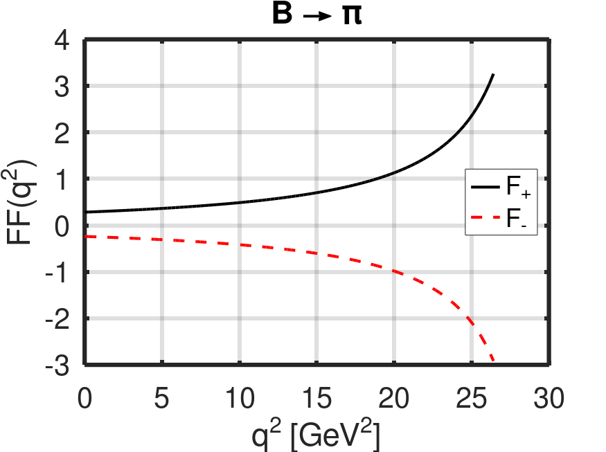
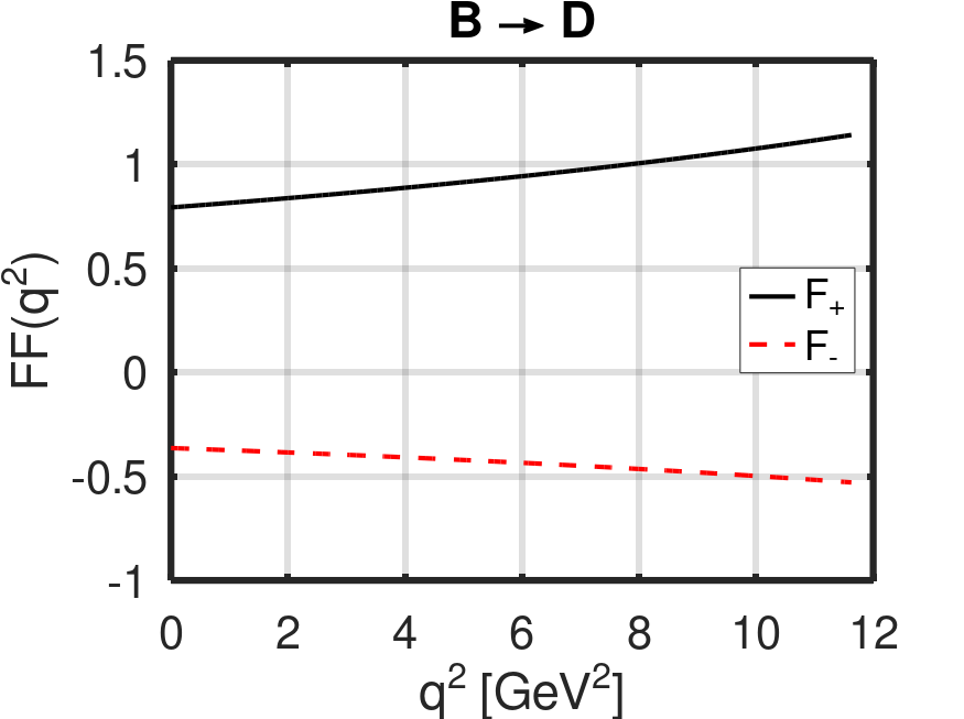
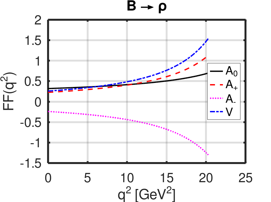
Figure 2: Form factors of transitions which determine the investigated decays.

The evaluation of hadronic form factors within the CCQM proceeds via standard computation techniques based on evaluation of the corresponding Feynman diagrams. For $B\rightarrow PS$ and $B\rightarrow V$ the transition the form factors are given by

$$F_{+}\left(q^{2}\right)P^{\mu}+F_{-}\left(q^{2}\right)q^{\mu}=$$

$$\hskip 56.9055pt=\frac{3g_{B}g_{H}}{4\pi^{2}}\int\frac{d^{4}k}{4\pi^{2}i}\widetilde{\varPhi}_{B}\left[-\left(k+w_{b}p_{B}\right)^{2}\right]\widetilde{\varPhi}_{H}\left[-\left(k+w_{q_{i}}p_{H}\right)^{2}\right]$$

$$\hskip 71.13188pt\times\mathrm{Tr}\left[S_{q_{i}}\left(k+p_{H}\right)O^{\mu}S_{b}\left(k+p_{B}\right)\gamma^{5}S_{q_{s}}\left(k\right)\gamma^{5}\right],$$

$$\frac{\epsilon_{H\nu}^{*}}{m_{B}+m_{H}}[-g^{\mu\nu}PqA_{0}\left(q^{2}\right)+P^{\mu}P^{\nu}A_{+}\left(q^{2}\right)$$

$$+q^{\mu}P^{\nu}A_{-}\left(q^{2}\right)+i\varepsilon^{\mu\nu\alpha\beta}P_{\alpha}q_{\beta}V\left(q^{2}\right)]=$$

$$\hskip 56.9055pt=\frac{3g_{B}g_{H}}{4\pi^{2}}\int\frac{d^{4}k}{4\pi^{2}i}\widetilde{\varPhi}_{B}\left[-\left(k+w_{b}p_{B}\right)^{2}\right]\widetilde{\varPhi}_{H}\left[-\left(k+w_{q_{i}}p_{H}\right)^{2}\right]$$

$$\hskip 71.13188pt\times\mathrm{Tr}\left[S_{q_{i}}\left(k+p_{H}\right)O^{\mu}S_{b}\left(k+p_{B}\right)\gamma^{5}S_{q_{s}}\left(k\right)\epsilon_{H\mu}\gamma^{\mu}\right].$$

Here $q_{s}$ and $q_{i}$ denote the spectator and the interacting quark of $H$ respectively ($H$ being $PS$ or $V$), $S$ represents quark propagators and $\epsilon_{H}$ the polarization vector of $H\equiv V$. Giving the vertex functions the above-mentioned Gaussian form and writing the propagators in the Schwinger representation, one performs the loop integration and applies the infrared cutoff in the integration over the Schwinger parameters, this last integration being done numerically. The model parameters were determined in our previous works [23, 18] and their numerical values are

$\varLambda_{B}$	$\varLambda_{D}$	$\varLambda_{D^{*}}$	$\varLambda_{D_{s}}$	$\varLambda_{D_{s}^{*}}$	$\varLambda_{\pi}$	$\varLambda_{\rho}$	$m_{b}$	$m_{s}$	$m_{q}$	$\lambda$
$1.96$	$1.60$	$1.53$	$1.75$	$1.56$	$0.87$	$0.61$	$5.04$	$0.428$	$0.241$	$0.181$

Table 2: CCQM parameters. Values are in GeV.

The predicted behavior of form factors in four studied transitions is shown in Fig. 2.

4 Results, conclusion

	Process	Diagram	$\mathcal{B}_{\mathrm{CCQM}}/\mathrm{E}$		$\mathcal{B}_{\mathrm{PDG}}/\mathrm{E}$	$\mathrm{E}$
1	$B^{0}\rightarrow D^{-}+\pi^{+}$	$D_{1}$	$5.34\pm 0.27$		$2.52\pm 0.13$	$10^{-3}$
2	$B^{0}\rightarrow\pi^{-}+D^{+}$	$D_{1}$	$11.19\pm 0.56$		$7.4\pm 1.3$	$10^{-7}$
3	$B^{0}\rightarrow\pi^{-}+D_{s}^{+}$	$D_{1}$	$3.48\pm 0.17$		$2.16\pm 0.26$	$10^{-5}$
4	$B^{+}\rightarrow\pi^{0}+D_{s}^{+}$	$D_{1}$	$1.88\pm 0.09$		$1.6\pm 0.5$	$10^{-5}$
5	$B^{0}\rightarrow D^{-}+\rho^{+}$	$D_{1}$	$14.06\pm 0.70$		$7.6\pm 1.2$	$10^{-3}$
6	$B^{0}\rightarrow\pi^{-}+D_{s}^{*+}$	$D_{1}$	$3.66\pm 0.18$		$2.1\pm 0.4$	$10^{-5}$
7	$B^{+}\rightarrow\pi^{0}+D^{*+}$	$D_{1}$	$0.804\pm 0.04$		$<3.6$	$10^{-6}$
8	$B^{+}\rightarrow\pi^{0}+D_{s}^{*+}$	$D_{1}$	$0.197\pm 0.01$		$<2.6$	$10^{-4}$
9	$B^{0}\rightarrow D^{*-}+\pi^{+}$	$D_{1}$	$4.74\pm 0.24$		$2.74\pm 0.13$	$10^{-3}$
10	$B^{0}\rightarrow\rho^{-}+D_{s}^{+}$	$D_{1}$	$2.76\pm 0.14$		$<2.4$	$10^{-5}$
11	$B^{+}\rightarrow\rho^{0}+D_{s}^{+}$	$D_{1}$	$0.149\pm 0.01$		$<3.0$	$10^{-4}$
12	$B^{0}\rightarrow D^{*-}+\rho^{+}$	$D_{1}$	$14.58\pm 0.73$		$6.8\pm 0.9$	$10^{-3}$
13	$B^{0}\rightarrow\rho^{-}+D_{s}^{*+}$	$D_{1}$	$5.09\pm 0.25$		$4.1\pm 1.3$	$10^{-5}$
14	$B^{+}\rightarrow\rho^{0}+D_{s}^{*+}$	$D_{1}$	$0.275\pm 0.01$		$<4.0$	$10^{-4}$
15	$B^{0}\rightarrow\pi^{0}+\overline{D}^{0}$	$D_{2}$	$0.085\pm 0.00$		$2.63\pm 0.14$	$10^{-4}$
16	$B^{0}\rightarrow\pi^{0}+\overline{D}^{*0}$	$D_{2}$	$1.13\pm 0.06$		$2.2\pm 0.6$	$10^{-4}$
17	$B^{0}\rightarrow\rho^{0}+\overline{D}^{0}$	$D_{2}$	$0.675\pm 0.03$		$3.21\pm 0.21$	$10^{-4}$
18	$B^{0}\rightarrow\rho^{0}+\overline{D}^{*0}$	$D_{2}$	$1.50\pm 0.08$		$<5.1$	$10^{-4}$
19	$B^{+}\rightarrow\overline{D}^{0}+\pi^{+}$	$D_{3}$	$3.89\pm 0.19$		$4.68\pm 0.13$	$10^{-3}$
20	$B^{+}\rightarrow\overline{D}^{0}+\rho^{+}$	$D_{3}$	$1.83\pm 0.09$		$1.34\pm 0.18$	$10^{-2}$
21	$B^{+}\rightarrow\overline{D}^{*0}+\pi^{+}$	$D_{3}$	$7.60\pm 0.38$		$4.9\pm 0.17$	$10^{-3}$
22	$B^{+}\rightarrow\overline{D}^{*0}+\rho^{+}$	$D_{3}$	$11.75\pm 0.59$		$9.8\pm 1.7$	$10^{-3}$

Table 3: Computed branching fractions compared with experimental measurements [24].

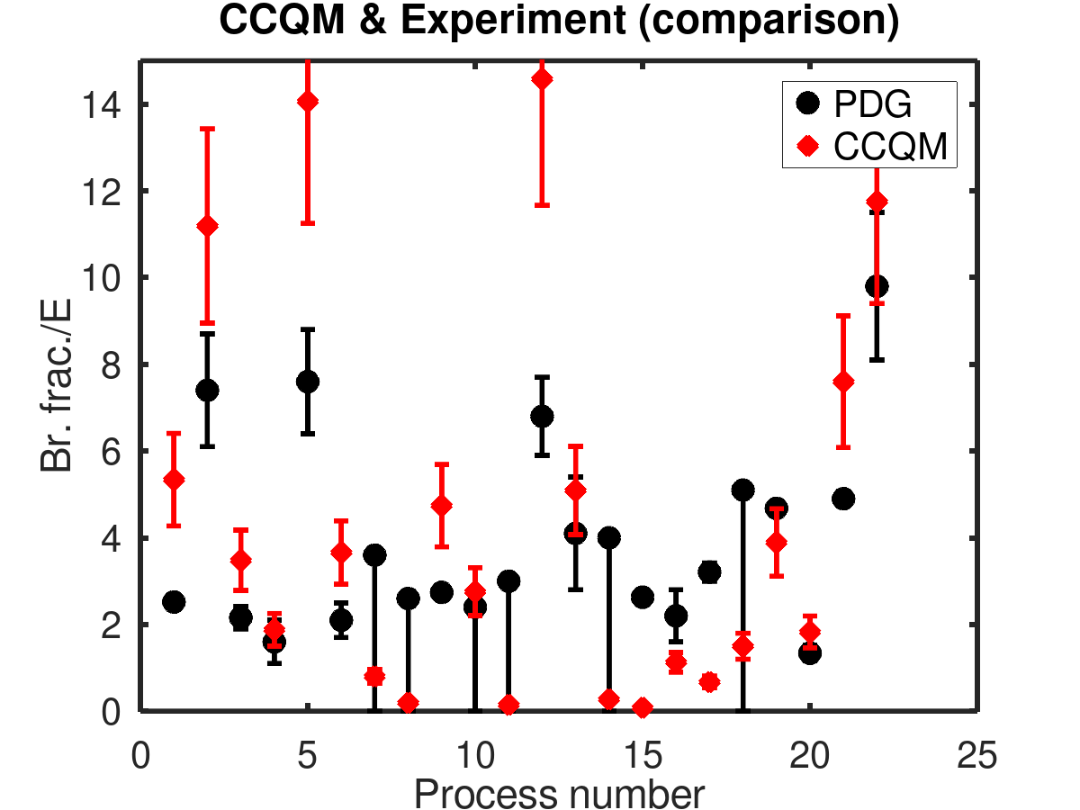
Figure 3: CCQM branching fraction predictions compared with the experimental values listed in the PDG [24]. Processes are numbered as in Tab. 3.

Our results are summarized in Table 3, the error on branching fractions is estimated to be 20%. The precision of the description of the experimental data is limited, as seen in Fig 3. The central values of the CCQM numbers are in agreement with those measurements which provide upper limits and in two other cases they lay inside 1$\sigma$ error of the measured value. For the rest, the CCQM provides mostly fair estimates of the experimental numbers, usually within the factor of two. However, also in these situations the difference in terms of standard deviations can be large, if the measured point has a small error. From this point of view large deviations are seen for color-suppressed processes (15)(17) and for those with $B\rightarrow D^{\left(*\right)}$ transition (1)(9)(21). Since the factorization assumption has no solid justification for the color-suppressed decays we address, we attribute the observe difference in (15)(17) to its breaking. Concerning processes (1)(9)(21), they have rather small experimental errors which may partly explain the large differences in terms of sigmas. One may also notice that they share the same set of form factors which implies correlation in their behavior and one indeed observes important overestimation also for other $B\rightarrow D^{\left(*\right)}$ processes, e.g. (5)(12). Actually, an overestimation is seen for almost all $D_{1}$ and $D_{3}$ decays (with the exception of (19)), the overestimation is just more pronounced for some processes than for others. Such systematic shift is somewhat surprising, but we are not the first to observe it, see [25, 26]. The authors of [27] notice the same behavior in similar decays too. They argue that it is difficult to provide a solid explanation within the Standard Model and thus propose new physics mechanisms. Our results seem to confirm their observations, which they label as “novel puzzle”. New physics explanations are also investigated in [28]. The comparison of our results with those of other authors is shown in Table 4.

Decay mode	our results	[25]	[28]
$B^{0}\rightarrow D^{-}\pi^{+}$	$5.34\pm 0.27$	$3.93_{-0.42}^{+0.43}$	$4.74_{-0.69}^{+0.61}$
$B^{0}\rightarrow D^{*-}\pi^{+}$	$4.74\pm 0.24$	$3.45_{-0.50}^{+0.53}$	$4.26_{-0.80}^{+0.75}$
$B^{0}\rightarrow D^{-}\rho^{+}$	$14.06\pm 0.70$	$10.42_{-1.20}^{+1.24}$	$12.28_{-1.63}^{+1.40}$
$B^{0}\rightarrow D^{*-}\rho^{+}$	$14.58\pm 0.73$	$9.24_{-0.71}^{+0.72}$	$11.61_{-2.01}^{+1.88}$

Table 4: Comparison of theoretical predictions for chosen branching fractions (in units $10^{-3}$).

References

• [1] E.Β Waheed etΒ al. Study of $\overline{B}{}^{0}\rightarrow D^{+}h^{-}(h=K/\pi)$ decays at Belle. 11 2021.
• [2] Roel Aaij etΒ al. Measurement of the branching fraction of the ${{B}^{0}}{\rightarrow}{{D}^{+}_{s}}{{\pi}^{-}}$ decay. Eur. Phys. J. C, 81(4):314, 2021.
• [3] Bernard Aubert etΒ al. Evidence for the Rare Decay $B^{+}\to D^{+}_{s}\pi^{0}$. Phys. Rev. Lett., 98:171801, 2007.
• [4] Bernard Aubert etΒ al. Branching fraction measurement of $B^{0}\to D^{(*)}+\pi^{-}$, $B^{-}\to D^{(*)}0\pi^{-}$ and isospin analysis of $\bar{B}\to D^{(*)}\pi$ decays. Phys. Rev. D, 75:031101, 2007.
• [5] Bernard Aubert etΒ al. Measurement of the absolute branching fractions $B$ to Dpi, D*pi, $D^{pi}$ with a missing mass method. Phys. Rev. D, 74:111102, 2006.
• [6] Roel Aaij etΒ al. Dalitz plot analysis of $B^{0}\to\overline{D}^{0}\pi^{+}\pi^{-}$ decays. Phys. Rev. D, 92(3):032002, 2015.
• [7] S.Β E. Csorna etΒ al. Measurements of the branching fractions and helicity amplitudes in $B\to D^{*}\rho$ decays. Phys. Rev. D, 67:112002, 2003.
• [8] M.Β S. Alam etΒ al. Exclusive hadronic B decays to charm and charmonium final states. Phys. Rev. D, 50:43–68, 1994.
• [9] M.Β Beneke, G.Β Buchalla, M.Β Neubert, and ChristopherΒ T. Sachrajda. QCD factorization for exclusive, nonleptonic B meson decays: General arguments and the case of heavy light final states. Nucl. Phys. B, 591:313–418, 2000.
• [10] Stanislav Dubnicka, AnnaΒ Z. Dubnickova, Aidos Issadykov, MikhailΒ A. Ivanov, and Andrej Liptaj. Study of $B_{c}$ decays into charmonia and $D$ mesons. Phys. Rev. D, 96(7):076017, 2017.
• [11] Stanislav Dubnicka, AnnaΒ Z. Dubnickova, MikhailΒ A. Ivanov, and Andrej Liptaj. Decays Bsβ†’J/ψ+Ξ·β†’subscriptπ΅π‘ π½πœ“πœ‚B_{s}\rightarrow J/\psi+\eta and Bsβ†’J/ψ+Ξ·β€²β†’subscriptπ΅π‘ π½πœ“superscriptπœ‚β€²B_{s}\rightarrow J/\psi+\eta^{\prime} in the framework of covariant quark model. Phys. Rev. D, 87:074201, 2013.
• [12] MikhailΒ A. Ivanov, JurgenΒ G. KΓΆrner, SergeyΒ G. Kovalenko, Pietro Santorelli, and GozyalΒ G. Saidullaeva. Form factors for semileptonic, nonleptonic and rare $B\,(B_{s})$ meson decays. Phys. Rev. D, 85:034004, 2012.
• [13] MichailΒ A. Ivanov, J.Β G. KΓΆrner, and O.Β N. Pakhomova. The Nonleptonic decays $B^{+}_{c}\to D^{+}_{s}\bar{D}^{0}$ and $B^{+}_{c}\to D^{+}_{s}D^{0}$ in a relativistic quark model. Phys. Lett. B, 555:189–196, 2003.
• [14] MikhailΒ A. Ivanov, JurgenΒ G. KΓΆrner, and Pietro Santorelli. Exclusive semileptonic and nonleptonic decays of the $B_{c}$ meson. Phys. Rev. D, 73:054024, 2006.
• [15] Matthias Neubert and AlexeyΒ A. Petrov. Comments on color suppressed hadronic B decays. Phys. Lett. B, 519:50–56, 2001.
• [16] Sebastien Descotes-Genon, Tobias Hurth, Joaquim Matias, and Javier Virto. Optimizing the basis of $B\to K^{*}ll$ observables in the full kinematic range. JHEP, 05:137, 2013.
• [17] Georges Aad etΒ al. Study of $B_{c}^{+}\to J/\psi D_{s}^{+}$ and $B_{c}^{+}\to J/\psi D_{s}^{*+}$ decays in $pp$ collisions at $\sqrt{s}=13$ TeV with the ATLAS detector. 3 2022.
• [18] Gurjav Ganbold, Thomas Gutsche, MikhailΒ A. Ivanov, and ValeryΒ E. Lyubovitskij. On the meson mass spectrum in the covariant confined quark model. J. Phys. G, 42(7):075002, 2015.
• [19] B.Β Jouvet. On the meaning of Fermi coupling. Nuovo Cim., 3:1133–1135, 1956.
• [20] Abdus Salam. Lagrangian theory of composite particles. Nuovo Cim., 25:224–227, 1962.
• [21] Steven Weinberg. Elementary particle theory of composite particles. Phys. Rev., 130:776–783, 1963.
• [22] Tanja Branz, Amand Faessler, Thomas Gutsche, MikhailΒ A. Ivanov, JurgenΒ G. KΓΆrner, and ValeryΒ E. Lyubovitskij. Relativistic constituent quark model with infrared confinement. Phys. Rev. D, 81:034010, 2010.
• [23] MikhailΒ A. Ivanov, JurgenΒ G. KΓΆrner, and ChanΒ T. Tran. Exclusive decays $b\to\ell^{-}\bar{\nu}$ and $b\to d^{(\ast)}\ell^{-}\bar{\nu}$ in the covariant quark model. Phys. Rev. D, 92(11):114022, 2015.
• [24] P.Β A. Zyla etΒ al. Review of Particle Physics. PTEP, 2020(8):083C01, 2020.
• [25] Tobias Huber, Susanne KrΓ€nkl, and Xin-Qiang Li. Two-body non-leptonic heavy-to-heavy decays at NNLO in QCD factorization. JHEP, 09:112, 2016.
• [26] Marzia Bordone, Nico Gubernari, Tobias Huber, Martin Jung, and Danny van Dyk. A puzzle in $\bar{B}_{(s)}^{0}\to D_{(s)}^{(*)+}\{\pi^{-},K^{-}\}$ decays and extraction of the $f_{s}/f_{d}$ fragmentation fraction. Eur. Phys. J. C, 80(10):951, 2020.
• [27] Syuhei Iguro and Teppei Kitahara. Implications for new physics from a novel puzzle in BΒ―(s)0β†’D(s)(βˆ—)+​{Ο€βˆ’,Kβˆ’}β†’superscriptsubscript¯𝐡𝑠0subscriptsuperscript𝐷limit-fromβˆ—π‘ superscriptπœ‹superscript𝐾\bar{B}_{(s)}^{0}\to D^{(\ast)+}_{(s)}\{\pi^{-},K^{-}\} decays. Phys. Rev. D, 102(7):071701, 2020.
• [28] Fang-Min Cai, Wei-Jun Deng, Xin-Qiang Li, and Ya-Dong Yang. Probing new physics in class-I B-meson decays into heavy-light final states. JHEP, 10:235, 2021.