BOOSTING PRUNED NETWORKS WITH LINEAR OVER-PARAMETERIZATION
Abstract
Structured pruning is a popular technique for reducing the computational cost and memory footprint of neural networks by removing channels. It often leads to a decrease in network accuracy, which can be restored through fine-tuning. However, as the pruning ratio increases, it becomes progressively more difficult to restore the accuracy of the trimmed network. To overcome this challenge, we propose a method that linearly over-parameterizes the compact layers, increasing the number of learnable parameters, and re-parameterizes them back to their original layers after fine-tuning, therefore contributing to better accuracy restoration. Similarity-preserving knowledge distillation is exploited to maintain the feature extraction ability of the expanded layers. Our method can be easily integrated without additional technology, making it compatible and can effectively benefit the pruning process for existing pruning techniques. Our approach outperforms fine-tuning on CIFAR-10 and ImageNet under different pruning strategies, particularly when dealing with large pruning ratios.
Index Terms— structured pruning, fine-tuning, over-parameterization, knowledge distillation
1 Introduction
Network pruning [1, 2, 3, 4], including structured [5, 6] and non-structured pruning [7, 8], is a widely used technique for reducing the computational complexity and memory usage of deep learning models by removing “unimportant” weights. However, these process often results in a significant drop in model accuracy. As the pruning ratio increases, it becomes increasingly challenging to restore the accuracy of the trimmed network. To address the issue of accuracy degradation, He et al. [9] reconstructed the outputs with remaining channels with linear least squares and avoided the process of fine-tuning. Zhu et al. [10] proposed an automated gradual pruning strategy in which pruning and fine-tuning are carried out alternately to prune the network gradually. However, previous fine-tuning methods either bypass the fine-tuning process or aim to alleviate the accuracy drop rather than focusing on the accuracy recovery during fine-tuning.
In this paper, we address this challenge by leveraging linear over-parameterization [11, 12], an approach designed for training compact neural networks from scratch. Linear over-parameterization generally expands linear layer of the compact network into multiple consecutive linear layers without nonlinear operations and contracts it back to the original structure after training. However, over-parameterization for fine-tuning after model pruning faces two problems: 1) the loss of information due to the removal of “unimportant” weights, and 2) the difficulty in gathering valuable features during fine-tuning. Facing these problems, we leverage similarity-preserving knowledge distillation [13, 14] to guide the fine-tuning of the over-parameterized network. In conclusion, our approach can better recover precision than vanilla fine-tuning, and maintain the representation ability during pruning and fine-tuning. Comprehensive experiments show that it outperforms existing pruning methods, particularly with large pruning ratios. When the pruning ratio increases to an extreme 95.52%, our method achieves 2.04% higher accuracy restoration than fine-tuning itself.
2 METHOD
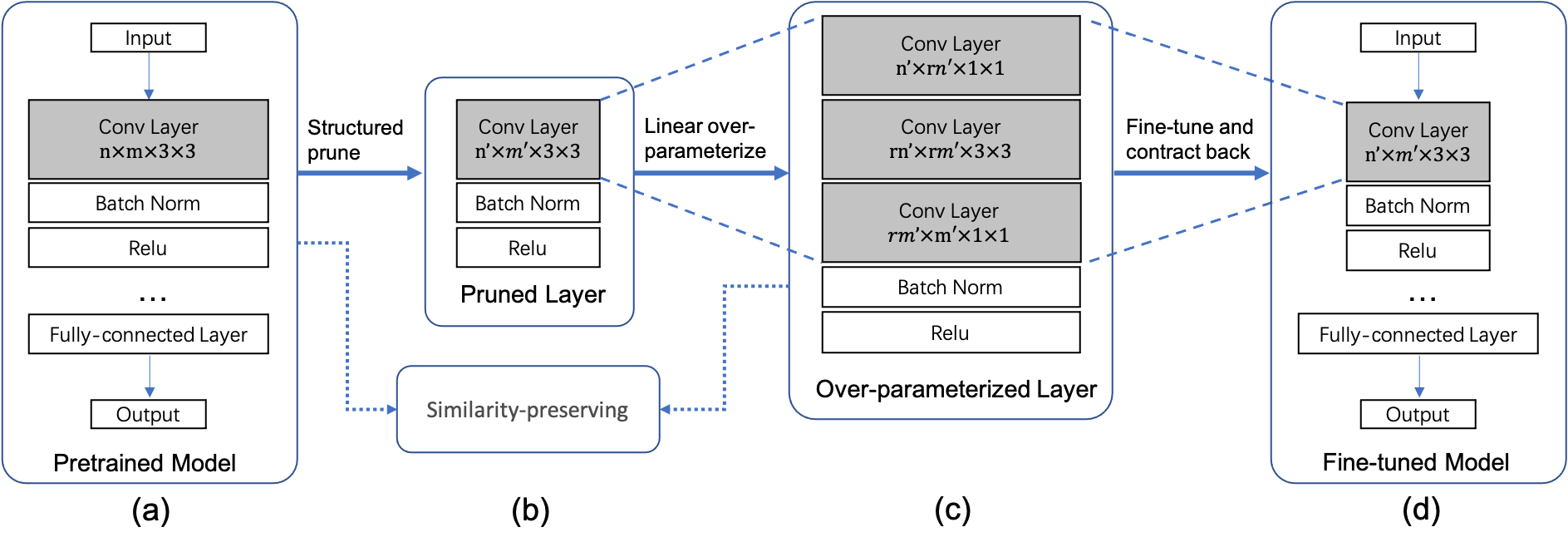
An overview of our proposed approach is illustrated in Fig. 1. The pretrained network undergoes a sequential process of structural pruning, linear over-parameterization, fine-tuning, and contraction to achieve the final slim model. During fine-tuning, similarity-preserving knowledge distillation is introduced to preserve feature extraction ability.
2.1 Expand Layers
Expanding convolutional layers. In this section, the filters of a convolutional layer are represented as , where and denote the number of input and output channels, and the kernel size. For a convolutional layer, Guo et al. [11] proposed to over-parameterize it into 3 consecutive layers: a convolution; a one; and another one (Fig. 1(c)). Based on that, for , we define the output channel number of the first layer as and the output channel number of the intermediate layer as with an expansion rate .
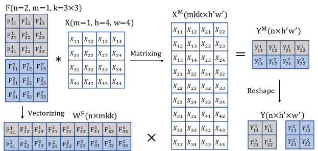
For a input tensor with height and width , the convolution can be formulated as
| (1) | ||||
where is the corresponding output tensor, and are the height and width of output tensor , is the unrolled matrix representation of the input tensor , and is the matrix representation of the convolutional filters . Fig. 2 provides an illustration of this process. Based on formula 1, a layer can be expanded linearly by replacing one matrix with matrices multiplied in succession.
More specifically, the matrix multiplication is formulated as
| (2) | ||||
Based on formula 2, the expanded layers are determined by matrix solving. More specifically, and are randomly initialized, so the weight of can be determined by matrix decomposition. This process can be formulated as
| (3) | ||||
where indicates the right inverse of and , the left inverse of . After similarity-preserving guided fine-tuning, the decomposed parameters go through matrix reconstruction following the decomposition pathway into the compact shape (Fig. 1(d)). To expand a convolutional layer with padding , we apply padding in the first layer of the expanded unit while not padding the remaining layers. To handle a stride , we set the stride of the middle layer to and that of the others to 1.
Expanding depthwise convolutional layers. To expand the depthwise convolutional layers, we set the group parameter of the expanded layers same as the original layer, then the normal convolutional expansion strategy is applied on these three consecutive layers within each group. This makes the expanded layers equivalent to the original ones for each group.
Expanding fully-connected layers. As for a fully-connected layer, we can directly expand a linear layer with input and output dimensions into linear layers as
| (4) |
We allocate the weights of the expanding layers by randomly initializing of them and calculating the weight of the remaining -th layer by matrix decomposition.
| (5) | ||||
For convenience, we denote and in Eq. 4 to get Eq. 5. In practice, considering the computational complexity of fully-connected layers, we expand each layer into only two or three layers with a small expansion rate.
Existence of left and right inverses. The left and right inverses of matrices need to be computed in Eq. 3 and Eq. 5 so they must exist. In our work, all matrices that need determining the inverses are initialized randomly. Considering matrix , the necessary and sufficient condition for the existence of its right inverse is and , i.e., matrix is row full rank. As is randomly initialized with normal distribution, the inverse can be determined after we remove the last columns. Under these circumstances, we can compare their full rank probability as
| (6) |
Feng et al. [15] has proved that a rational random matrix has full rank with probability 1, that is, . Thus with Eq. 6 we get and its right inverse exist certainly. In this way, in order to ensure the existence of a matrix’s left and right inverse, what we need to do is to control the expansion rate. E.g., when we expand a fully-connected layer to , if we randomly initialize and calculate , we should ensure . Conversely, we should set the value .
2.2 Feature Extraction Preserving
Over-parameterization will destroy the stable feature extraction ability of the pretrained and pruned model. To handle this, similarity-preserving knowledge distillation [13] is applied. Given an input mini-batch, it denotes the activation map produced by the un-pruned network T (teacher network) at a particular layer as and the activation map produced by the over-parameterized network S (student network) at the last corresponding expand layer as . The distillation loss, an L2 regularization penalty, is applied. First, let . Then we get
| (7) |
| (8) |
| (9) |
| (10) |
The similarity-preserving knowledge distillation loss is designed as
| (11) |
where collects the layer pairs. Finally, the total loss for student network training is defined as
| (12) |
where denotes the loss function of vision task, is the ground truth, and is the input mini-batch. denotes the output from over-parameterized network S.
3 EXPERIMENTS
3.1 Implemented Details
In our experiments, we evaluate the proposed strategies on CIFAR-10 [16] and ImageNet [17]. The image size is 3232 for CIFAR-10 and 224224 for ImageNet, and trained with the batch size 256. We apply the ADMM strategy and compare the effect of our proposed method and other fine-tuning methods in the fine-tuning stage. To demonstrate the generalization of our proposed method, we conduct comparative experiments under other pruning strategies, including AMC [18], HRank [19], ThiNet [20], and EagleEye [21].
3.2 Results
3.2.1 Results for ADMM
After removing the less important parameters, there are two styles of fine-tuning: (1) retaining the remaining weights and (2) training the pruned structure from scratch. For the first case, we fine-tune the network for 150 epochs, with a learning rate of 0.01 decay by a factor 10 at epochs 60, 100, and 120. We retrain the network for 280 epochs for the second case, with a learning rate of 0.1 decayed by a factor 10 at epochs 100, 160, 210, and 250.
In this section, we compare the proposed method with four other competing methods. These methods include: 1) training from scratch, 2) ExpandNets [11], 3) vanilla distillation, where we retrain the reinitialized model with similarity-preserving knowledge distillation loss, and 4) vanilla fine-tuning.
| ADMM | Percent of weights removed (%) | ||||
|---|---|---|---|---|---|
| 0 | 68.37 | 78.23 | 94.80 | 98.66 | |
| Training from scratch | 94.17 | 86.22 | 83.47 | 72.08 | 49.08 |
| ExpandNets | 94.36 | 87.61 | 84.99 | 75.14 | 51.25 |
| Vanilla distillation | 94.17 | 87.80 | 85.03 | 75.03 | 51.31 |
| Vanilla fine-tuning | 94.17 | 93.27 | 92.74 | 86.03 | 54.39 |
| Ours | 94.17 | 93.31 | 93.26 | 87.97 | 56.88 |
MobileNetV2 on CIFAR-10. Tab. 1 presents the results for all methods. Our method outperforms the other methods in terms of accuracy restoration, especially when the pruning ratio is relatively large. ExpandNets and vanilla distillation produce similar results, which is consistent with [11]. Both methods perform much worse than vanilla fine-tuning, indicating that applying over-parameterization and knowledge distillation alone is not sufficient for pruning.
ResNet-50 on ImageNet. For ResNet-50 on ImageNet, the top-1 accuracy results are shown in Tab. 2, which are consistent with the conclusions above.
| ADMM | Percent of weights removed (%) | ||||
|---|---|---|---|---|---|
| 0 | 28.37 | 54.25 | 71.23 | 93.18 | |
| Training from scratch | 79.18 | 74.14 | 71.42 | 67.39 | 56.79 |
| ExpandNets | 78.87 | 74.28 | 73.82 | 71.06 | 58.07 |
| Vanilla distillation | 79.18 | 75.32 | 73.69 | 72.61 | 58.65 |
| Vanilla fine-tuning | 79.18 | 77.63 | 75.03 | 72.88 | 62.47 |
| Ours | 79.18 | 77.47 | 75.76 | 73.36 | 64.08 |
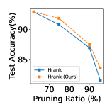
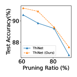
3.2.2 Results for other pruning strategies
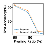
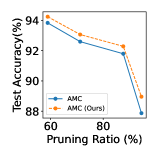
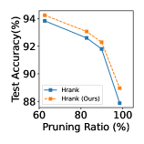
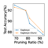
In this section, we apply various pruning strategies to prove the reliability of the proposed method. And we compare the proposed with Vanilla fine-tuning. Fig. 3, Fig. 4 and Tab. 3 show that in most cases, our proposed method is superior to Vanilla fine-tuning.
| AMC | Percent of weights removed (%) | |||
|---|---|---|---|---|
| 0 | 52.64 | 63.28 | 95.63 | |
| Vanilla fine-tuning | 80.10 | 74.60 | 72.30 | 50.52 |
| Ours | 80.10 | 75.50 | 73.15 | 51.20 |
3.3 Ablation Study
Similarity-preserving knowledge distillation. The ablation study is carried out on CIFAR-10 with MobileNetV2. The results are shown in Tab. 4. Over-parameterized fine-tuning without knowledge distillation performs slightly better than vanilla fine-tuning but is unstable. When we use similarity-preserving knowledge distillation, our method can achieve better and more stable performance.
| ADMM | Distillation | Percent of weights removed (%) | ||||
|---|---|---|---|---|---|---|
| 0 | 68.37 | 89.80 | 94.80 | 98.66 | ||
| Vanilla fine-tuning | w/o KD | 94.17 | 93.27 | 91.67 | 86.03 | 54.39 |
| Ours | w/o KD | 94.17 | 93.25 | 91.83 | 86.28 | 54.92 |
| Ours | w/ KD | 94.17 | 93.31 | 92.07 | 87.97 | 56.88 |
Expansion rate. We investigated the contribution of expanding the fully-connected layers in our experiments, and the results are presented in Tab. 5. A suitable expansion rate, such as 3, can enhance the overall performance of the network. Conversely, a large value, such as 5, may overly complicate the network and hinder convergence.
| Rate | Expand FC | FLOPs | Params | Acc(%) |
|---|---|---|---|---|
| 0 | w/o Expand FC | 43.298M | 215.642K | 88.91 |
| 2 | w Expand FC | 313.736M | 1.675M | 89.43 |
| 3 | w/o Expand FC | 591.660M | 3.127M | 90.15 |
| 3 | w Expand FC | 591.665M | 3.132M | 90.12 |
| 5 | w/o Expand FC | 1.392G | 7.282M | 90.07 |
| 5 | w Expand FC | 1.392G | 7.293M | 90.13 |
4 CONCLUSION
In this paper, we propose a linear over-parameterization approach to improve accuracy restoration in structurally pruned neural networks. It’s achieved by fine-tuning the over-parameterized layers with increased parameters of the compact networks, during which similarity-preserving knowledge is exploited to maintain the feature extraction ability. Comprehensive comparisons of CIFAR-10 and ImageNet datasets show that our approach outperforms fine-tuning, especially with large pruning ratios. Our method benefits the fine-tuning stage of pruning and synergizes with techniques in the areas of pruning optimization, weight importance evaluation, and adaptive pruning ratios. Consequently, it can be concurrently applied with these methods to enhance the overall effectiveness of pruning.
References
- [1] Shangqian Gao, Feihu Huang, Weidong Cai, and Heng Huang, “Network pruning via performance maximization,” in Proceedings of the IEEE/CVF Conference on Computer Vision and Pattern Recognition, 2021, pp. 9270–9280.
- [2] Tailin Liang, John Glossner, Lei Wang, Shaobo Shi, and Xiaotong Zhang, “Pruning and quantization for deep neural network acceleration: A survey,” Neurocomputing, vol. 461, pp. 370–403, 2021.
- [3] Wenxiao Wang, Minghao Chen, Shuai Zhao, Long Chen, Jinming Hu, Haifeng Liu, Deng Cai, Xiaofei He, and Wei Liu, “Accelerate cnns from three dimensions: A comprehensive pruning framework,” in International Conference on Machine Learning. PMLR, 2021, pp. 10717–10726.
- [4] Ruichi Yu, Ang Li, Chun-Fu Chen, Jui-Hsin Lai, Vlad I Morariu, Xintong Han, Mingfei Gao, Ching-Yung Lin, and Larry S Davis, “Nisp: Pruning networks using neuron importance score propagation,” in Proceedings of the IEEE conference on computer vision and pattern recognition, 2018, pp. 9194–9203.
- [5] Xiaohan Ding, Guiguang Ding, Yuchen Guo, and Jungong Han, “Centripetal sgd for pruning very deep convolutional networks with complicated structure,” in Proceedings of the IEEE/CVF conference on computer vision and pattern recognition, 2019, pp. 4943–4953.
- [6] Hao Li, Asim Kadav, Igor Durdanovic, Hanan Samet, and Hans Peter Graf, “Pruning filters for efficient convnets,” arXiv preprint arXiv:1608.08710, 2016.
- [7] Xin Dong, Shangyu Chen, and Sinno Pan, “Learning to prune deep neural networks via layer-wise optimal brain surgeon,” Advances in Neural Information Processing Systems, vol. 30, 2017.
- [8] Namhoon Lee, Thalaiyasingam Ajanthan, Stephen Gould, and Philip HS Torr, “A signal propagation perspective for pruning neural networks at initialization,” arXiv preprint arXiv:1906.06307, 2019.
- [9] Yihui He, Xiangyu Zhang, and Jian Sun, “Channel pruning for accelerating very deep neural networks,” in Proceedings of the IEEE international conference on computer vision, 2017.
- [10] Michael Zhu and Suyog Gupta, “To prune, or not to prune: exploring the efficacy of pruning for model compression,” arXiv preprint arXiv:1710.01878, 2017.
- [11] Shuxuan Guo, Jose M Alvarez, and Mathieu Salzmann, “Expandnets: Linear over-parameterization to train compact convolutional networks,” arXiv preprint arXiv:1811.10495, 2018.
- [12] Xiaohan Ding, Xiangyu Zhang, Ningning Ma, Jungong Han, Guiguang Ding, and Jian Sun, “Repvgg: Making vgg-style convnets great again,” in Proceedings of the IEEE/CVF Conference on Computer Vision and Pattern Recognition, 2021.
- [13] Frederick Tung and Greg Mori, “Similarity-preserving knowledge distillation,” in Proceedings of the IEEE/CVF International Conference on Computer Vision, 2019.
- [14] Jie Zhang, Chen Chen, Bo Li, Lingjuan Lyu, Shuang Wu, Shouhong Ding, Chunhua Shen, and Chao Wu, “DENSE: Data-free one-shot federated learning,” in Advances in Neural Information Processing Systems, Alice H. Oh, Alekh Agarwal, Danielle Belgrave, and Kyunghyun Cho, Eds., 2022.
- [15] Xinlong Feng and Zhinan Zhang, “The rank of a random matrix,” Applied mathematics and computation, vol. 185, no. 1, pp. 689–694, 2007.
- [16] Alex Krizhevsky, Geoffrey Hinton, et al., “Learning multiple layers of features from tiny images,” Tech. Rep., 2009.
- [17] Jia Deng, Wei Dong, Richard Socher, Li-Jia Li, Kai Li, and Li Fei-Fei, “Imagenet: A large-scale hierarchical image database,” in 2009 IEEE conference on computer vision and pattern recognition. Ieee, 2009.
- [18] Yihui He, Ji Lin, Zhijian Liu, Hanrui Wang, Li-Jia Li, and Song Han, “Amc: Automl for model compression and acceleration on mobile devices,” in Proceedings of the European conference on computer vision (ECCV), 2018, pp. 784–800.
- [19] Mingbao Lin, Rongrong Ji, Yan Wang, Yichen Zhang, Baochang Zhang, Yonghong Tian, and Ling Shao, “Hrank: Filter pruning using high-rank feature map,” in Proceedings of the IEEE/CVF conference on computer vision and pattern recognition, 2020, pp. 1529–1538.
- [20] Jian-Hao Luo, Jianxin Wu, and Weiyao Lin, “Thinet: A filter level pruning method for deep neural network compression,” in Proceedings of the IEEE international conference on computer vision, 2017.
- [21] Bailin Li, Bowen Wu, Jiang Su, and Guangrun Wang, “Eagleeye: Fast sub-net evaluation for efficient neural network pruning,” in European conference on computer vision. Springer, 2020, pp. 639–654.