ATLASGAL-selected massive clumps in the inner Galaxy. X. Observations of atomic carbon at 492 GHz

Abstract

Context. While high-mass stars are key drivers of the evolution of galaxies, how they form and interact with the surrounding gas remains not fully understood. To shed light on this overarching issue, we have been performing a multi-telescope campaign to observe carbon species in $\sim$100 massive clumps identified by the ATLASGAL survey (Top100 sample). Our targets constitute a representative sample of high-mass star-forming regions with a wide range of masses ($\sim$20–10⁴ $M_{\odot}$), bolometric luminosities ($\sim$60–10⁶ $L_{\odot}$), and evolutionary stages (70 $\mu$m weak, infrared weak, infrared bright, and H ii region sources).

Aims. We aim to probe the physical conditions of [C i]-traced gas in the Top100 sample based on APEX [C i] 492 GHz single-pointing observations. This is the first of a series of papers presenting results from our [C ii] and [C i] campaign.

Methods. To determine physical properties such as the temperature, density, and column density, we combined the obtained [C i] 492 GHz spectra with APEX observations of [C i] 809 GHz and ¹³CO(2–1), as well as with other multi-wavelength data, and employed both local thermodynamic equilibrium (LTE) and non-LTE methods.

Results. Our 98 sources are clearly detected in [C i] 492 GHz emission, and the observed integrated intensities and line widths tend to increase toward evolved stages of star formation. In addition to these “main” components that are associated with the Top100 sample, 41 emission and two absorption features are identified by their velocities toward 28 and two lines of sight respectively as “secondary” components. The secondary components have systematically smaller integrated intensities and line widths than the main components. We found that [C i] 492 GHz and ¹³CO(2–1) are well correlated with the ¹³CO(2–1)-to-[C i] 492 GHz integrated intensity ratio varying from 0.2 to 5.3. In addition, we derived the H₂-to-[C i] conversion factor, $X$(C i), by dividing 870 $\mu$m-based H₂ column densities by the observed [C i] 492 GHz integrated intensities and found that $X$(C i) (in units of cm^-2 (K km s^-1)^-1) ranges from 2.3 $\times$ 10²⁰ to 1.3 $\times$ 10²² with a median of 1.7 $\times$ 10²¹. In contrast to the strong correlation with ¹³CO(2–1), [C i] 492 GHz has a scattered relation with the 870 $\mu$m-traced molecular gas. Finally, we performed LTE and non-LTE analyses of the [C i] 492 GHz and 809 GHz data for a sub-set of the Top100 sample and inferred that [C i] emission likely originates from warm (kinetic temperature $\gtrsim$ 60 K), optically thin (opacity $<$ 0.5), and highly pressurized (thermal pressure $\sim$ a few (10⁵–10⁸) K cm^-3) regions.

Conclusions. Our [C i] 492 GHz survey demonstrates that [C i] 492 GHz is prevalent in the inner Galaxy and traces not only massive clumps, but also non-star-forming relatively diffuse gas. The strong correlation between [C i] 492 GHz and ¹³CO(2–1) indicates that they probe similar conditions, and the observed variations in the intensity ratio of the two transitions likely reflect local conditions of the interstellar medium. The scattered relation between [C i] 492 GHz and the 870 $\mu$m-based molecular gas, on the other hand, implies that [C i] 492 GHz and ¹³CO(2–1) probe warm molecular gas that surrounds denser and colder clumps traced by 870 $\mu$m emission.

1 Introduction

High-mass stars play a key role in the evolution of galaxies (e.g., Kennicutt & Evans 2012). For instance, massive stars inject a substantial amount of radiative and mechanical energy into the surrounding gas via ultraviolet (UV) radiation fields, stellar outflows/winds, and supernova explosions. This stellar feedback has been argued to be critical for regulating star formation in galaxies (e.g., Cox 1981; Silk 1997; Ostriker et al. 2010; Hopkins et al. 2014). In addition, high-mass stars enrich the interstellar medium with heavy elements throughout their lives, driving the chemical evolution of galaxies (e.g., Matteucci 2021).

Despite their importance, how high-mass stars form and interact with the surrounding gas is not yet fully understood (e.g., Motte et al. 2018). One of the challenges has been that massive star-forming regions tend to be widely separated and located far awary from us due to the rarity of high-mass stars. Furthermore, high-mass stars reach the main sequence while deeply embedded in their parental molecular clouds, preventing us from probing the early stage of star formation with traditional optical and near-infrared (NIR) observations. To overcome these difficulties and provide a comprehensive census of high-mass star-forming regions, a number of Galactic plane surveys at far-infrared (FIR) and submillimeter (submm) wavelengths have been performed in recent years, including the APEX Telescope Large Area Survey of the Galaxy (ATLASGAL; Schuller et al. 2009). ATLASGAL is a 870 $\mu$m survey of the inner Galaxy (covering $|l|<60^{\circ}$ with $|b|<1.5^{\circ}$ and $280^{\circ}<l<300^{\circ}$ with $-2^{\circ}<b<1^{\circ}$) conducted with the Atacama Pathfinder EXperiment (APEX) 12 m submillimeter telescope in Chile. This survey identified $\sim$10⁴ massive clumps (e.g., Contreras et al. 2013; Csengeri et al. 2014; Urquhart et al. 2014), and the brightest $\sim$100 of them (Top100 hereafter) have been a subject of various follow-up studies, e.g., Giannetti et al. (2014) (investigating CO depletion and isotopic ratios), Csengeri et al. (2016) (probing SiO-traced shocked gas), Kim et al. (2017) (searching for H ii regions), and König et al. (2017) (characterizing physical properties based on dust continuum emission). More specifically, König et al. (2017) constructed dust spectral energy distributions (SEDs) from 8 $\mu$m to 870 $\mu$m and measured dust temperatures and fluxes. Along with distance information, the authors then estimated clump masses, luminosities, and column densities on $\sim$19^′′ scales. These dust-based analyses showed that the Top100 sample could be divided into four groups, i.e., 70 $\mu$m weak sources (70w), mid-infrared (MIR) weak sources (IRw), MIR-bright sources (IRb), and MIR-bright sources associated with radio continuum emission (H ii regions), and the dust temperature and bolometric luminosity increase along this sequence, implying that the Top100 sample represents different evolutionary stages of high-mass star formation.

We have been conducting a multi-telescope campaign for observing carbon species in the Top100 clumps to address the following questions: (1) What are the physical conditions of the interstellar medium leading to high-mass star formation? (2) How do the energetics of gas surrounding massive young stellar objects and protostellar objects vary as the sources evolve? Carbon is a critical ingredient in the evolution of the interstellar medium (e.g., Henning & Salama 1998). In its different forms, i.e., C⁺, C⁰, and CO, it is one of the primary coolants and provides a powerful diagnostic tool for examining the physical conditions and energetics of gas. For example, [C ii], [C i], and low-$J$ CO transitions (upper $J$ $\lesssim$ 4) can be used to probe the properties of photodissociation regions, while mid- and high-$J$ CO lines can trace shock-heated gas (e.g., Pon et al. 2014; Lee et al. 2019). Among these carbon phases, atomic carbon has received relatively little attention, mainly because [C i] fine-structure transitions are typically fainter than low-$J$ CO emission and are heavily affected by atmospheric absorption. Theoretically, atomic carbon is expected to be abundant at the surfaces of molecular clouds (e.g., Langer 1976), but subsequent observations have shown that [C i] emission is widespread throughout the clouds, invoking an interest in [C i] emission as a tracer of total gas mass (e.g., Frerking et al. 1989; Schilke et al. 1995; Kramer et al. 2008; Oka et al. 2001; Shimajiri et al. 2013).

This is the first of a series of papers presenting results from our [C ii] and [C i] campaign for the Top100 sources. As a pilot study, we here focus on examining the physical conditions of [C i]-traced gas based on APEX [C i] 492 GHz single-pointing observations, and the two science questions described above will be addressed with more data in forthcoming papers. The organization of this paper is as follows. In Sect. 2, we present APEX [C i] and ¹³CO(2–1) observations of the Top100 sources and describe the determination of line parameters (including central velocities and line widths) via Gaussian fitting. The observed properties of [C i] 492 GHz are probed across different evolutionary stages of high-mass star formation (Sect. 3) and are compared to molecular gas tracers (e.g., ¹³CO(2–1) and dust-based H₂; Sect. 4). In addition, the [C i] 492 GHz and 809 GHz data for a small sub-set of the Top100 sources are analyzed to derive the physical conditions of [C i]-traced gas (Sect. 5). Finally, we discuss our results and summarize main findings in Sect. 6.

2 Observations and data reduction

2.1 [C i] 492 GHz

Single-pointing observations of the [C i] ${}^{3}P_{1}$–${}^{3}P_{0}$ transition at 492.16065 GHz were made toward 98 of the Top100 sources using the APEX FLASH⁺ (First Light APEX Submillimeter Heterodyne instrument; Klein et al. 2014) receiver in 2016 (project IDs: M0039-97 and M0013-98). Two different off positions were observed in the total power mode to avoid contamination, while additional observations were performed in the wobbler mode to accurately measure continuum levels. The characteristic of the observed sources, including locations, distances, and classifications, are summarized in Table LABEL:t:appendix_table1. The obtained spectra were processed with the GILDAS CLASS software and were converted into units of main-beam brightness temperature ($T_{\rm MB}$) using a forward efficiency ($F_{\rm eff}$) of 0.95 and a main-beam efficiency ($B_{\rm eff}$) of 0.46 based on Mars observations. The final spectra on 13^′′ scales were smoothed to a velocity resolution of 0.46 km s^-1 and have a root-mean-square (rms) noise level of 0.1–0.6 K (median $\sim$ 0.3 K).

2.2 [C i] 809 GHz

Nine of the Top100 sources were mapped in the [C i] ${}^{3}P_{2}$–${}^{3}P_{1}$ transition at 809.34197 GHz using the APEX CHAMP⁺ (Carbon Heterodyne Array of the MPIfR; Güsten et al. 2008) instrument in 2013 (project ID: M0010-92). The mapping was made in the On-The-Fly (OTF) mode with a coverage of 1.6^′ $\times$ 1.6^′, and the observed sources are marked in Table LABEL:t:appendix_table1. The GILDAS CLASS software was employed for data reduction, and the processed data cubes were translated into the $T_{\rm MB}$ units by adopting $F_{\rm eff}$ = 0.95 and $B_{\rm eff}$ = 0.38 based on Mars observations. The final data on 8^′′ scales were smoothed to a velocity resolution of 0.70 km s^-1 and have a median rms noise level of $\sim$1 K.

2.3 ¹³CO(2–1)

The 98 sources in our [C i] 492 GHz survey were also observed in the ¹³CO(2–1) transition at 220.39868 GHz (single-pointing) using the APEX PI230 receiver in 2016 (project ID: M0024-97). Unlike the [C i] 492 GHz observations, only one off position was observed for each source in the total power mode. The obtained ¹³CO(2–1) data were reduced using the GILDAS CLASS software and were converted into the $T_{\rm MB}$ units by assuming $F_{\rm eff}$ = 0.95 and $B_{\rm eff}$ = 0.66 (Tang et al. 2018). The final science-ready spectra have a resolution of 30^′′ and a rms noise level of 0.04–0.14 K (median $\sim$ 0.06 K) per 0.66 km s^-1 channel.

2.4 Deriving line parameters

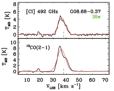
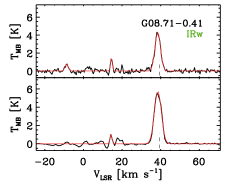
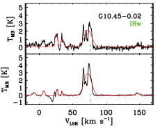
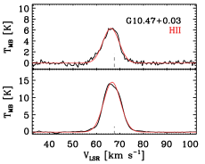
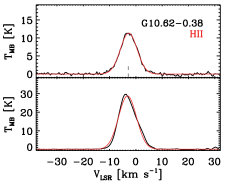
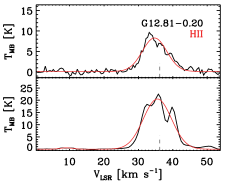
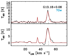
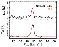
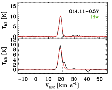
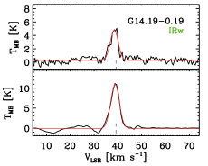
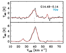
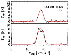
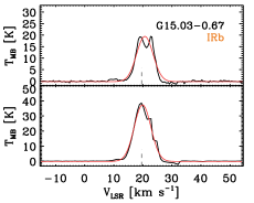
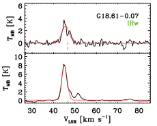
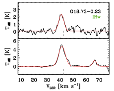
Figure 14: APEX [C i] 492 GHz and ¹³CO(2–1) spectra (top and bottom for each panel). The fitted Gaussians are overlaid in red, and the source velocities are indicated as the gray dashed lines. Several spectra (in particular ¹³CO(2–1)) show absorption features, which most likely result from contaminated reference positions. On the other hand, [C i]-absorbing components toward G43.17$+$0.01 and G330.95$-$0.18 are labelled with the word “ABS”.

While the observed [C i] 809 GHz spectra can be approximated as single Gaussians, the [C i] 492 GHz and ¹³CO(2–1) spectra often show complex shapes with multiple components (Appendix B). For our analyses, we identified individual components by fitting Gaussian functions to the final spectra and estimated line parameters such as central velocities and full width at half maximum (FWHMs). When two components are close to each other, we examined the difference between their central velocities and considered them as one component if the difference is smaller than the sum of their FWHMs. In addition, we calculated the integrated intensity ($I$([C i]) or $I$(¹³CO)) of each identified component by integrating the emission over a velocity range over which the component is clearly detected. For [C i] 809 GHz, we smoothed the cubes and used the spectra that were extracted at a resolution of 13^′′ to compare with the [C i] 492 GHz data (Sect. 5). The final [C i] and ¹³CO(2–1) spectra with the fitted Gaussians are shown in Fig. 14, and the derived line parameters and integrated intensities are presented in Table LABEL:t:appendix_table2.

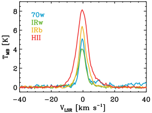
Figure 1: Average [C i] 492 GHz spectra of the four evolutionary groups (70w, IRw, IRb, and H ii region groups in blue, green, yellow, and red). To derive these spectra, sources with contaminated reference positions were excluded.

3 Observational results

In this section, we mainly discuss the observed properties of [C i] 492 GHz (integrated intensities and FWHMs) and how they vary in a diversity of environments.

3.1 [C i] 492 GHz detection rate

We regard components whose peak-to-rms ratios are equal to or higher than five as detections. With this threshold, we found that all 98 sources are detected in [C i] 492 GHz emission. The exact breakdown of the sources is as follows: 14, 31, 31, and 22 for the 70w, IRw, IRb, and H ii region groups respectively. These different evolutionary groups have comparable median distances ($\sim$4 kpc) and [C i] 492 GHz sensitivities ($\sim$0.3 K), making comparisons of the groups straightforward. In addition to the main components that are directly associated with the Top100 sources, secondary components are detected in both emission and absorption (Fig. B.1): 41 emission components toward 28 lines of sight and two absorption components toward two lines of sight. Throughout this paper, we refer to these components as “diffuse clouds”, since they likely trace colder and less dense gas than the main 98 components.

3.2 Average [C i] 492 GHz spectra

To examine how [C i] 492 GHz changes across different environments, we first derived average spectra of the four evolutionary groups by shifting the observed spectra to a central velocity of 0 km s^-1 based on the source velocities and stacking them (Fig. 1). For this, 94 sources with clean reference positions were considered (12, 30, 30, and 22 for the 70w, IRw, IRb, and H ii region groups respectively).

Fig. 1 shows that the characteristics of [C i] 492 GHz emission systematically change across the four evolutionary stages in terms of brightness and line width. Specifically, the peak temperature increases from 5.8 K to 7.8 K for the IRb and H ii region groups, while the 70w spectrum has a slightly higher peak than the IRw spectrum (4.7 K versus 3.8 K). On the other hand, the FWHM increases toward more evolved stages: 4.3, 5.6, 5.9, and 8.4 km s^-1 for the 70w, IRw, IRb, and H ii region groups. The peak temperature and FWHM values here were estimated from Gaussian fitting of the average spectra.

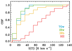
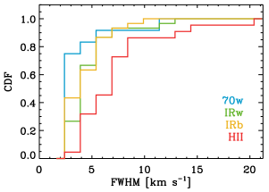
Figure 2: CDFs of the [C i] 492 GHz integrated intensity (top) and FWHM (bottom). For both plots, the 70w, IRw, IRb, and H ii region groups are shown in blue, green, yellow, and red respectively.

3.3 Integrated intensities and line widths of the main components

Next we probed how statistically different [C i] 492 GHz properties are between the evolutionary stages by constructing cumulative distribution functions (CDFs) of the integrated intensity and FWHM for the main components (Fig. 2). Like in Sect. 3.2, we used the 94 sources with clean reference positions only.

The top panel of Fig. 2 suggests that the 70w, IRw, and IRb groups have comparable distributions of the integrated intensity, while the H ii region group has systematically higher values (median $I$(C i) $\sim$ 23, 21, 26, and 67 K km s^-1 for the 70w, IRw, IRb, and H ii region group respectively). This result is supported by two-sided Kolmogorov-Smirnov (K-S) tests at a significance level of 5%, where only the H ii region group is found to be statistically distinct from the rest. Similarly, we found that the 70w and H ii region groups have the smallest and largest FWHMs, while the IRw and IRb groups have intermediate FWHMs (Fig. 2 bottom): median FWHM $\sim$ 3.7, 4.6, 4.4, and 7.0 km s^-1 for the 70w, IRw, IRb, and H ii region group respectively. This conclusion again agrees with K-S tests where the 70w group is found to be statistically different from the IRw and H ii region groups and the H ii region group stands out against the rest.

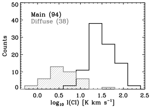
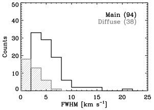
Figure 3: Histograms of the [C i] 492 GHz integrated intensity (top) and FWHM (bottom). The distributions of the 94 main components and 38 diffuse cloud components are shown in black and gray respectively.

3.4 Comparison between the main and diffuse cloud components

As noted in Sect. 3.1, 41 components are detected along 28 lines of sight as secondary emission components. In comparison to the main components that are associated with the Top100 sources, these secondaries have systematically smaller values of the [C i] 492 GHz integrated intensity and line width (Fig. 3). For example, the median $I$(C i) is 29 K km s^-1 and 4 K km s^-1 for the main and diffuse cloud components respectively, while the median FWHM is 5 km s^-1 and 2 km s^-1. For these estimates and the histograms in Fig. 3, spectra with clean reference positions were used (94 and 38 for the main and diffuse cloud components respectively).

In summary, our APEX survey suggests that [C i] 492 GHz is ubiquitous and traces not only massive dense clumps, but also non-star-forming relatively diffuse gas. The observed integrated intensities and FWHMs systematically vary across different environments, which is likely driven by local conditions of the interstellar medium.

Table 1: Types of [C i] and ¹³CO detections.

	Type 0(a)	Type 1(a)	Type 2(a)
[C i] detection	✓	✗	✓
13CO detection	✓	✓	✗
70w	14 (10)	0	0
IRw	31 (21)	0	0
IRb	31 (21)	0	0
H ii region	22 (22)	0	0
Diffuse(b)	35 (23)	45 (42)	5 (3)
Total	133 (97)	45 (42)	5 (3)

Notes. ^(a) The values in parenthesis are the numbers of detections that have clean reference positions. ^(b) G22.37$+$0.45 shows two components in [C i] 492 GHz, which are sufficiently close to be considered as one component in ¹³CO(2–1). When we compared [C i] 492 GHz to ¹³CO(2–1), we therefore used a sum of the two components in [C i] 492 GHz for this source. Because of this, the total number of diffuse cloud components detected in [C i] 492 GHz is 40 in this table, as opposed to 41 as we mentioned in Sect. 3.4.

4 Relation between [C i] 492 GHz and molecular gas tracers

From which part of a molecular cloud [C i] 492 GHz emission arises has long been a subject of debate. Considering the small difference between the ionization threshold of C⁰ (11.26 eV) and the dissociation threshold of CO (11.09 eV), C⁰ is expected to form a narrow layer between C⁺ and CO, limiting its usefulness as a tracer of total gas mass. However, a significant body of research has revealed that this expectation could be wrong and C⁰ could exist deep inside molecular clouds (e.g., Frerking et al. 1989; Schilke et al. 1995; Kramer et al. 2008). For example, the proportionality between the [C i] 492 GHz and low-$J$ ¹³CO integrated intensities has often been interpreted as evidence of the widespread [C i] 492 GHz emission throughout molecular clouds (e.g., Keene et al. 1997; Oka et al. 2001; Shimajiri et al. 2013; Izumi et al. 2021). In this section, we try to shed light on the origin of [C i] 492 GHz emission by examining a relation between [C i] 492 GHz and molecular gas tracers (including ¹³CO(2–1) and 870 $\mu$m-based H₂).

4.1 [C i] 492 GHz and ¹³CO(2–1)

4.1.1 Classification of [C i] and ¹³CO detections

We here probe the relation between [C i] 492 GHz and ¹³CO(2–1) in detail. First, we started our analysis by classifying the [C i] and ¹³CO data into three types: (1) Type 0 where [C i] 492 GHz and ¹³CO(2–1) are detected; (2) Type 1 where only ¹³CO(2–1) is detected; (3) Type 2 where only [C i] 492 GHz is detected. The breakdown of each type is summarized in Table 1.

Among 139 components that are seen in [C i] 492 GHz emission, 133 show clear ¹³CO(2–1) detections, implying a good correspondence between [C i] 492 GHz and ¹³CO(2–1) in general. On the other hand, 45 secondary components are newly detected in ¹³CO(2–1) only, which is in contrast to a handful number of components seen in [C i] 492 GHz only (5). This striking difference partially results from the higher sensitivity of the ¹³CO(2–1) data (Sect. 2).

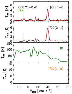
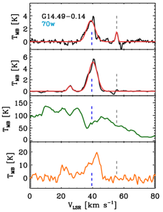
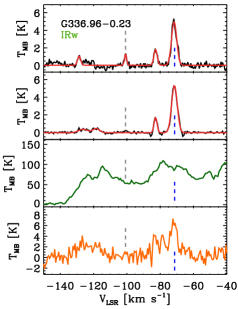
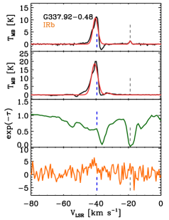
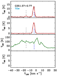
Figure 4: Comparison between [C i] 492 GHz (black), ¹³CO(2–1) (black), H i (green), and ¹²CO(1–0) (orange) for five sources. For H i, the absorption spectrum from Brown et al. (2014) is shown for G337.92$-$0.48, while SGPS data are presented for the remaining sources. In addition, ¹²CO(1–0) spectra from the FUGIN (G14.49$-$0.14) and Mopra (G336.96$-$0.23 and G337.92$-$0.48) surveys are used. Over the [C i] 492 GHz and ¹³CO(2–1) spectra, the fitted Gaussians are overlaid in red. Finally, the source velocities and the secondary components that are seen in [C i] 492 GHz without corresponding ¹³CO(2–1) detections are indicated in blue and gray respectively.

4.1.2 [C i] 492 GHz as a tracer of “CO-dark” molecular gas

The [C i] 492 GHz components without corresponding ¹³CO(2–1) detections can be candidates for “CO-dark” molecular gas and require an in-depth look. In Fig. 4, we compare [C i] 492 GHz, ¹³CO(2–1), H i, and ¹²CO(1–0) for the five sources toward which [C i] components without association with ¹³CO(2–1) emission are identified (indicated as gray dashed lines). For G08.71$-$0.41, G14.49$-$0.14, G336.96$-$0.23, and G351.57$+$0.77, H i is seen in emission, and 2^′-scale spectra from the Southern Galactic Plane Survey (SGPS; McClure-Griffiths et al. 2005) are shown. On the contrary, absorption features are detected toward G337.92$-$0.48, and the H i absorption spectrum from Brown et al. (2014) is presented. Finally, for ¹²CO(1–0), 20^′′- and 36^′′-scale spectra from the FOREST Unbiased Galactic plane Imaging survey with the Nobeyama 45 m telescope (FUGIN; Umemoto et al. 2017) and the Mopra southern Galactic plane survey (Braiding et al. 2018) are used.

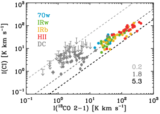
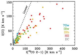
Figure 5: Comparison between the [C i] 492 GHz and ¹³CO(2–1) integrated intensities. All three types (Types 0, 1, and 2; Sect 4.1.1) are used here, and the 70w, IRw, IRb, H ii region groups, and diffuse cloud components are shown in different colors. For the Type 1, upper limits were calculated by $N.C$([C i]) $\times$ [C i] 492 GHz 5$\sigma$ $\times$ $\Delta\varv$([C i]) where $N.C$([C i]) is the number of [C i] channels over which ¹³CO is detected and $\Delta\varv$([C i]) is the velocity resolution of the [C i] spectra. A similar calculation was done for the Type 2, but using the number of ¹³CO channels over which [C i] is detected, ¹³CO 5$\sigma$, and velocity resolution of the ¹³CO spectra instead. These derived upper limits are indicated as the arrows. Left: log scale. The measured minimum, median, and maxium $I$(¹³CO)-to-$I$([C i]) ratios (0.2, 1.8, and 5.3) are indicated as the dashed lines in different shades of gray color. Right: linear scale. A linear one-to-one relation is shown as the black dashed line.

Fig. 4 shows that G08.71$-$0.41 and G14.49$-$0.14 likely suffer from bad reference positions in ¹³CO(2–1) at the velocities of our interest ($-$9 km s^-1 and 55 km s^-1 respectively), which means that ¹³CO(2–1) could have been detected. On the other hand, ¹³CO(2–1) is simply too faint at the velocities of our interest for G336.96$-$0.23, G337.92$-$0.48, and G351.57$+$0.77 ($-$101 km s^-1, $-$19 km s^-1, and $-$16 km s^-1 respectively), implying the $I$(¹³CO)-to-$I$([C i]) ratios lower than 0.7, 0.9, and 0.5 respectively. For these estimates, ¹³CO(2–1) 5$\sigma$ values for the velocity ranges where [C i] emission is integrated are considered. In general, Fig. 4 shows that H i is abundant toward the five sources. In particular, for G337.92$-$0.48, the [C i] component without associaiton with ¹³CO(2–1) emission corresponds to the strongest absorption feature, implying a substantial contribution from the cold H i . On the contrary, ¹²CO(1–0) is not detected at the velocities of our interest for G336.96$-$0.23 and G337.92$-$0.48 (rms of $\sim$1–2 K). These results suggest that the [C i] 492 GHz secondary components without corresponding ¹³CO(2–1) detections have a large amount of atomic gas and could trace “CO-dark” molecular gas. This conclusion, however, is drawn from a couple lines of sight and needs to be confirmed by extensive observations of [C i] 492 GHz, ¹³CO(2–1), and ¹²CO(1–0) with matching resolutions and sensitivities.

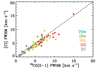
Figure 6: [C i] 492 GHz line width versus ¹³CO(2–1) line width. Only the Type 0 detections with simple spectra are shown here.

4.1.3 Correlation between the [C i] and ¹³CO integrated intensities

In Fig. 5, we show a comparison between the [C i] 492 GHz and ¹³CO(2–1) integrated intensities for all three types. To provide different perspectives, both linear and log versions are presented. For this comparison, we excluded 41 detections that suffer from bad reference positions in [C i] 492 GHz or ¹³CO(2–1) and used arrows to mark upper limits for the Types 1 and 2.

In general, we found that the [C i] 492 GHz and ¹³CO(2–1) integrated intensities are well correlated. For instance, the Type 0 detections have a strong correlation between [C i] 492 GHz and ¹³CO(2–1) with a Spearman rank correlation coefficient of 0.95. This suggests that [C i] 492 GHz and ¹³CO(2–1) arise from similar regions of the interstellar medium, which could be supported by comparable line widths of the two transitions (Fig. 6): the median of the absolute difference between the [C i] 492 GHz and ¹³CO(2–1) line widths is 0.8 km s^-1. Considering a factor of two larger resolution of the ¹³CO(2–1) data (13^′′ versus 30^′′), this difference in FWHM is surprisingly small. Finally, both [C i] 492 GHz and ¹³CO(2–1) are likely not too optically thick (Sect. 5.2; Urquhart et al. 2021), contributing to the good correlation between the two transitions.

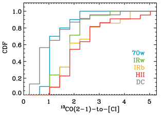
Figure 7: CDFs of the $I$(¹³CO)-to-$I$([C i]) ratio. The 70w, IRw, IRb, H ii region groups, and diffuse cloud components are shown in blue, green, yellow, red, and gray. For this plot, 97 Type 0 detections with clean off positions were considered.

4.1.4 Ratio of ¹³CO to [C i]

While [C i] 492 GHz and ¹³CO(2–1) are strongly correlated, the ratio of ¹³CO(2–1) to [C i] 492 GHz does vary, e.g., the $I$(¹³CO)-to-$I$([C i]) ratio ranges from 0.2 to 5.3 with a median of 1.8 (Fig. 5 left). These variations can be seen in Fig. 5 (right) as well, where the data points deviate from the linear one-to-one relation more significantly as the [C i] and ¹³CO integrated intensities increase beyond $\sim$50 K km s^-1. Considering that $I$([C i]) increases toward more evolved groups (Sect. 3.3), the systematic deviation from the linear one-to-one relation implies that the ratio of ¹³CO(2–1) to [C i] 492 GHz depends on the classification of the sources.

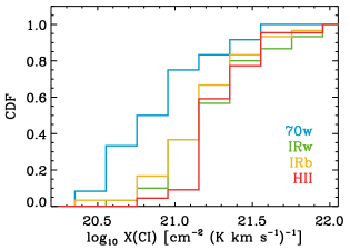
Figure 8: Left: $X$(C i) histogram. The median value of 1.7 $\times$ 10²¹ cm^-2 (K km s^-1)^-1 is indicated as the dashed line. Right: CDFs of the $X$(C i) factor (70w, IRw, IRb, and H ii region sources in blue, green, yellow, and red respectively).

To examine how the ratio of ¹³CO(2–1) to [C i] 492 GHz depends on the classification of the sources, we constructed CDFs of $I$(¹³CO)/$I$([C i]) for the 70w, IRw, IRb, H ii region, and diffuse cloud groups and found that the diffuse cloud and 70w groups have systematically lower ratios (Fig. 7). For example, the fraction of the sources with $I$(¹³CO)/$I$([C i]) $<$ 2 are 87%, 80%, 48%, 57%, and 41% for the diffuse cloud, 70w, IRw, IRb, and H ii region groups respectively. This conclusion is also supported by two-sided K-S tests, where the diffuse cloud and 70w groups are found to be drawn from the same distribution, while the null hypothesis is rejected at a significance level of 5% when the diffuse cloud components are compared against the IRw/IRb/H ii region groups.

The observed variations in the ¹³CO(2–1)-to-[C i] 492 GHz integrated intensity ratio most likely result from local conditions of gas and implies that the Top100 sources are in different stages of carbon phase transition (C⁺-, C⁰-, or CO-dominated). The exact stages of carbon phase transition, as well as the underlying physical and energetic conditions, will be examined in forthcoming papers where observations of important cooling lines ([C ii], [C i], [O i], and CO transitions) for the Top100 sources are analyzed using state-of-the-art models of photodissociation regions and shocks (e.g., Le Petit et al. 2006; Flower & Pineau des Forêts 2015).

4.2 [C i] 492 GHz and 870 $\mu$m-based H₂

4.2.1 $X$(C i) factor

In addition to ¹³CO(2–1), we examined a relation between [C i] 492 GHz and the total H₂ column density by calculating the ratio of $N$(H₂) to $I$([C i]) ($X$(C i) factor). For this calculation, we extracted the 870 $\mu$m-based $N$(H₂) estimates from König et al. (2017) for the 94 main components whose [C i] 492 GHz spectra have clean reference positions and scaled them by (13/19)² to compensate the difference in resolution (13^′′ and 19^′′ for [C i] 492 GHz and H₂ respectively; this scaling assumes that H₂ uniformly fills the 19^′′ beam). The derived $X$(C i) ranges from 2.3 $\times$ 10²⁰ to 1.3 $\times$ 10²² with a median of 1.7 $\times$ 10²¹ (in units of cm^-2 (K km s^-1)^-1; Fig. 8 left), and this median value is consistent with recent observations of the massive star-forming region RCW 38 (1.4 $\times$ 10²¹; Izumi et al. 2021), as well as predictions from numerical simulations ($\sim$10²¹; Offner et al. 2014; Glover et al. 2015).

While showing a Gaussian distribution with the well-defined peak of 1.7 $\times$ 10²¹, $X$(C i) has large variations (a factor of 55). To examine if there is any trend in these variations, we constructed CDFs for the four evolutionary groups (Fig. 8 right). The constructed CDFs show that the H ii region group has more sources with high $X$(C i) values. For example, sources with $X$(C i) $>$ 1.7 $\times$ 10²¹ constitute 77% of the H ii region group, while accounting for 25%, 57%, and 33% of the 70w, IRw, and IRb groups. When examined at a significance level of 5% for two-sided K-S tests, the H ii region group was found to be statistically different from the 70w and IRb groups.

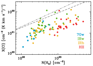
Figure 9: $X$(C i) versus $N$(H₂) (70w, IRw, IRb, and H ii region sources in blue, green, yellow, and red). The predicted relations, $X$(C i) = 8.4 $\times$ 10³ $N$(H₂)^0.79 ($G_{\rm UV}$ = 1 Draine field) and $X$(C i) = 1.2 $\times$ 10⁶ $N$(H₂)^0.69 ($G_{\rm UV}$ = 10 Draine field), by Offner et al. (2014) are shown in gray.

4.2.2 Dependence of $X$(C i) on $N$(H₂)

Sect. 4.2.1 showed that $N$(H₂) for a given $I$([C i]) is not constant and varies across the evolutionary groups. To better understand the origin of these variations, we examined how $X$(C i) changes with $N$(H₂) (Fig. 9) and found that $X$(C i) has a weak dependence on $N$(H₂) (Spearman’s rank correlation coefficient of 0.6; we did not attempt to perform least-squares fitting, since proper fitting is impossible without uncertainties in the H₂ column density). The same dependence of $X$(C i) on the H₂ column density was also found by Offner et al. (2014) and Izumi et al. (2021). In particular, Offner et al. (2014) performed hydrodynamic simulations of Galactic molecular clouds with two different UV radiation fields ($G_{\rm UV}$ = 1 and 10 Draine fields) and showed that $X$(C i) increases with $N$(H₂) $\gtrsim$ 10²² cm^-2 (gray lines in Fig. 9). This increase of $X$(C i) with $N$(H₂) was interpreted as a result of [C i] 492 GHz becoming optically thick and less sensitive to high H₂ column densities. In our case, however, [C i] 492 GHz is likely not too optically thick (Sect. 5). Our result could rather indicate the flattening of C⁰ abundance at high H₂ column densities, which can be verified by a comprehensive excitation study based on extensive [C i] 492 GHz and 809 GHz observations.

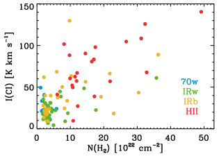
Figure 10: $I$([C i]) versus $N$(H₂) (70w, IRw, IRb, and H ii region sources in blue, green, yellow, and red).

4.2.3 Relation between $I$([C i]) and $N$(H₂)

The observed variations in $X$(C i) reflect a scattered relation between $I$([C i]) and $N$(H₂) (Fig. 10), which is in sharp contrast to the tight correlation between $I$([C i]) and $I$(¹³CO) (Fig. 5 right). While bearing in mind possible sources for the scatter (e.g., variations in the assumed properties of dust and gas, such as the dust opacity at 870 $\mu$m and dust-to-gas mass ratio), we take our result at face value and interpret it as a result of [C i] 492 GHz being a tracer of moderately dense molecular gas that is more closely associated with ¹³CO(2–1). Indeed, Duarte-Cabral et al. (2021) recently performed a cross-match between the ATLASGAL 870 $\mu$m and SEDIGISM ¹³CO(2–1) surveys and found that 4824 ATLASGAL clumps are enveloped within 1709 SEDIGISM clouds, implying that ¹³CO(2–1) probes the molecular gas that surrounds denser and colder clumps traced by 870 $\mu$m. Similarly, Plume et al. (2000) and Shimajiri et al. (2013) found that [C i] 492 GHz is poorly correlated with CS(1–0) and C¹⁸O(1–0) (dense molecular gas tracers) in Orion A. In general, our finding suggests that [C i] 492 GHz would not be a good tracer of total gas mass if the cloud mass is dominated by dense and cold molecular gas.

5 Physical conditions traced by [C i]

Two fine-structure transitions of [C i] at 492 GHz and 809 GHz are invaluable to constrain the physical properties of gas. For instance, in the optically thin regime, their flux ratio constrains the excitation temperature ($T_{\rm ex}$) as the integrated intensity is proportional to the upper state column density. In more general situations, including high optical depth cases, the physical properties of gas can be derived through escape probability radiative transfer models such as RADEX (van der Tak et al. 2007). In this section, we examine the physical conditions of [C i]-traced gas in a small sub-set of the Top100 sources by analyzing the [C i] 492 GHz and 809 GHz observations in the commonly adopted approximation of local thermodynamic equilibrium (LTE). Considering that what kind of the interstellar medium [C i] traces is not entirely clear, we perform a non-LTE calculation as well to evaluate the impact of sub-critical densities.

5.1 LTE calculation

As mentioned in Sect. 2.2, we observed nine sources in [C i] 809 GHz. To compare with the [C i] 492 GHz data, we smoothed the [C i] 809 GHz cubes and extracted spectra on 13^′′ scales from the pixels that correspond to the observed positions in our [C i] 492 GHz survey. The [C i] 809 GHz emission is detected in four sources, and the observed peak temperatures are summarized in Table 2.

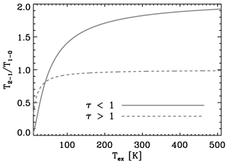
Figure 11: Ratio of the 809 GHz to 492 GHz peak temperature ($T_{2-1}$/$T_{1-0}$) as a function of the excitation temperature ($T_{\rm ex}$). Optically thin and thick cases are shown in solid and dashed lines.

Table 2: Properties of [C i] 492 GHz and 809 GHz.

Name	Class.	$T_{\rm peak,1-0}$	$T_{\rm peak,2-1}$	FWHM1-0	FWHM2-1	$T_{\rm ex}$	$\tau_{1-0}$	$\tau_{2-1}$	$N$(C)
		(K)	(K)	(km s-1)	(km s-1)	(K)			(1017 cm-2)
G24.63$+$0.17	IRw	4.4	9.5 $\downarrow$	3.0	$-$	510 $\downarrow$	0.01 $\uparrow$	0.02 $\uparrow$	3.1 $\downarrow$
G28.56$-$0.24	IRw	4.3	6.4 $\downarrow$	5.4	$-$	120 $\downarrow$	0.04 $\uparrow$	0.06 $\uparrow$	3.5 $\downarrow$
G337.17$-$0.03	IRw	3.5	4.3 $\downarrow$	7.4	$-$	72 $\downarrow$	0.06 $\uparrow$	0.08 $\uparrow$	3.5 $\downarrow$
G338.07$+$0.01	70w	2.4	4.1 $\downarrow$	11.4	$-$	196 $\downarrow$	0.01 $\uparrow$	0.02 $\uparrow$	5.5 $\downarrow$
G338.78$+$0.48	70w	5.1 $\uparrow$	6.7 $\downarrow$	4.9	$-$	$-$	$-$	$-$	$-$
G344.23$-$0.57	IRw	5.3	5.6	4.3	4.6	60${}_{-6}^{+11}$	0.11${}_{-0.02}^{+0.03}$	0.14${}_{-0.01}^{+0.02}$	3.3${}_{-0.1}^{+0.1}$
G345.00$-$0.23	H ii region	1.9	3.3	3.9	6.2	186${}_{-67}^{+107}$	0.01${}_{-0.005}^{+0.008}$	0.02${}_{-0.008}^{+0.009}$	1.6${}_{-0.1}^{+0.1}$
G345.49$+$0.32	H ii region	13.2	17.5	6.3	5.8	94${}_{-3}^{+4}$	0.17${}_{-0.01}^{+0.01}$	0.26${}_{-0.01}^{+0.01}$	14.2${}_{-0.1}^{+0.1}$
G345.51$+$0.35	IRb	10.4	9.6	4.5	5.4	49${}_{-2}^{+2}$	0.32${}_{-0.02}^{+0.02}$	0.35${}_{-0.01}^{+0.01}$	9.2${}_{-0.1}^{+0.1}$

Notes. The columns are as follows. Name: ATLASGAL source name; Class.: source classification based on König et al. (2017); $T_{\rm peak,1-0}$: [C i] 492 GHz peak main-beam brightness temperature; $T_{\rm peak,2-1}$: [C i] 809 GHz peak main-beam brightness temperature; FWHM_1-0: [C i] 492 GHz line width; FWHM_2-1: [C i] 809 GHz line width; $T_{\rm ex}$: excitation temperature; $\tau_{1-0}$: [C i] 492 GHz opacity; $\tau_{2-1}$: [C i] 809 GHz opacity; $N$(C): [C i] 492 GHz-based column density of atomic carbon. For the five sources where [C i] 492 GHz only is detected, the upper and lower limits on the relevant parameters are indicated as the downward and upward arrows. In the case of G338.78$+$0.48, the measured $T_{\rm peak,1-0}$ is most likely a lower limit, since its [C i] 492 GHz spectrum is affected by a contaminated reference position.

Given that the observed sources are dense clumps, we could assume LTE conditions and derive physical conditions including the excitation temperature, opacities at 492 GHz and 809 GHz ($\tau_{1-0}$ and $\tau_{2-1}$), and atomic carbon column density ($N$(C)) (Appendix C). But before the LTE calculation, we first explored how the ratio of the 809 GHz to 492 GHz peak main-beam brightenss temperature ($T_{2-1}$/$T_{1-0}$) changes with the excitation temperature in two extreme cases: optically thin and thick regimes. When $\tau\ll 1$, Eqs. (3) and (7) suggest that $T_{2-1}$/$T_{1-0}$ can be written as

$$\frac{T_{2-1}}{T_{1-0}}=2.1\leavevmode\nobreak\ \textrm{exp}\left(\frac{-23.6}{T_{\rm{ex}}}\right)\frac{\textrm{exp}(23.6/T_{\rm ex})-1}{\textrm{exp}(38.9/T_{\rm ex})-1}\frac{1-\textrm{exp}(-38.9/T_{\rm ex})}{1-\textrm{exp}(-23.6/T_{\rm ex})}.$$ (1)

On the other hand, when $\tau\gg 1$, $T_{2-1}$/$T_{1-0}$ can be written as

$$\frac{T_{2-1}}{T_{1-0}}=1.6\leavevmode\nobreak\ \frac{\textrm{exp}(23.6/T_{\rm ex})-1}{\textrm{exp}(38.9/T_{\rm ex})-1}.$$ (2)

Eqs. (1) and (2) are plotted as a function of the excitation temperature in Fig. 11.

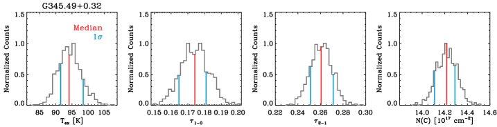
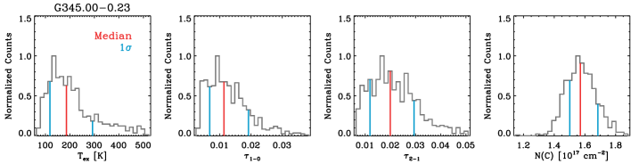
Figure 12: Normalized histograms of the MC-based parameters (top: G345.49$+$0.32; bottom: G345.00$-$0.23). The median values and 1$\sigma$ boundaries are indicated in red and blue.

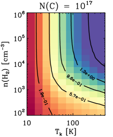
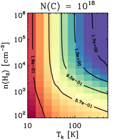
Figure 13: Predicted 809 GHz-to-492 GHz temperature ratios for $N$(C) = 10¹⁶, 10¹⁷, and 10¹⁸ cm^-2 (left, middle, and right respectively). In each plot, the overlaied contours range from 10% to 90% of the peak temperature ratio with 20% steps.

Fig. 11 shows interesting limiting behaviors. For example, the 809 GHz line would be twice as bright as the 492 GHz line (in temperature units) when the [C i]-emitting gas is warm ($k_{\rm B}T_{\rm ex}$ $\gg$ $h\nu_{2-1}$) and optically thin. On the other hand, the 809 GHz line would be about half as bright when the gas is cool ($T_{\rm ex}$ $\sim$ 10–20 K) and optically thick. The observed $T_{2-1}$/$T_{1-0}$ ranges from $\sim$0.9 to $\sim$1.7 (Table 2), suggesting that the [C i]-emitting gas is likely warm and optically thin.

To estimate $T_{\rm ex}$, $\tau_{1-0}$, $\tau_{2-1}$, $N$(C), and their associated 1$\sigma$ uncertainties, we performed Monte Carlo (MC) simulations where the [C i] spectra are perturbed 1000 times based on the rms values (Gaussian errors are assumed). Each perturbed spectrum is fitted with a Gaussian function to measure the peak temperature, and Eqs. (4), (5), and (10) are applied to the measured temperatures to derive $T_{\rm ex}$, $\tau_{1-0}$, $\tau_{2-1}$, and $N$(C). For our calculation of $N$(C), $\tau_{1-0}$ is used since it has a higher sensitivity than $\tau_{2-1}$. Finally, the distribution of each parameter is examined to estimate a median value, as well as $\pm$34% boundaries from the median (so that the data points within the boundaries are 68% of the total number). These median values and 1$\sigma$ boundaries are provided in Table 2, and the normalized histograms of the derived parameters for G345.49$+$0.32 and G340.00$-$0.23 are shown in Fig. 12 to demonstrate our calculation. We note that G345.00$-$0.23 has asymmetric distributions, leading to a large uncertainty in $T_{\rm ex}$ in particular. This is because the measured temperature ratio of 1.7 is on the asymptotic part of the $T_{2-1}$/$T_{1-0}$ versus $T_{\rm ex}$ curve (Fig. 11) and therefore a small change in the ratio can result in a large variation in $T_{\rm ex}$. For the five sources where [C i] 809 GHz is not detected, the lower and upper limits on the physical parameters are provided in Table 2.

Zmuidzinas et al. (1988) observed Galactic star-forming regions (OMC 1, NGC 2024, S140, DR 21(OH), W3, M17, and W51) in [C i] 492 GHz and 809 GHz and performed similar excitation analyses. Compared to Zmuidzinas et al. (1988) results (32–77 K), our excitation temperatures (49–186 K) are slightly higher. In particular, we found a tendency of higher temperatures for more evolved sources (94 K and 186 K for the two H ii region sources), though this needs to be verified by extensive [C i] 809 GHz observations in the future. Our optical depth values are, on the other hand, lower than Zmuidzinas et al. (1988), i.e., $\tau_{1-0}$ $\sim$ 0.01–0.32 versus 0.22–1.25.

Table 3: RADEX parameters for the individual sources.

	G344.23$-$0.57	G345.00$-$0.23	G345.49$+$0.32	G345.51$+$0.35
$T_{2-1}$/$T_{1-0}$(a)	1.06 (0.09)	1.74 (0.25)	1.33 (0.02)	0.92 (0.03)
$N$(C)(b) (1017 cm-2)	3.2	1.8	10	10
$T_{\rm k}$(c) (K)	57–500	136–500	136–324	57–324
	57	324	230	112
	132	140	133	120
$n$(H2)(c) (103 cm-3)	1–103	3–103	3–10	1–10
	20	100	7	2
	300	300	5	4
$P/k_{\rm B}$(c) (105 K cm-3)	3–600	20–5 $\times$ 103	10–14	2–6
	10	200	12	3
	200	103	2	1
$\tau_{1-0}$(c)	0.02–0.1	0.002–0.02	0.03–0.1	0.1–0.3
	0.09	0.006	0.06	0.2
	0.03	0.005	0.04	0.1
$\tau_{2-1}$(c)	0.10–0.12	0.008–0.03	0.20–0.21	0.36–0.39
	0.11	0.02	0.21	0.37
	0.01	0.01	0.01	0.01
$T_{1-0}$(c)	4.0–4.4	1.9–2.2	11.9–12.3	11.9–13.3
	4.1	2.0	12.1	12.7
	0.1	0.1	0.3	0.6
$T_{2-1}$(c)	4.0–4.7	3.2–3.7	15.8–16.4	11.0–12.5
	4.2	3.5	16.1	12.0
	0.2	0.2	0.4	0.6

Notes. ^(a) The observed temperature ratio and its 1$\sigma$ uncertainty (in parentheses). ^(b) The input $N$(C) for RADEX that is closest to the LTE-based $N$(C). ^(c) The RADEX parameters that are found to reproduce the observed temperature ratios within 1$\sigma$ uncertainties ($P/k_{\rm B}$ = thermal pressure). The ranges, median values, and 1$\sigma$ uncertainties are presented in rows.

5.2 Non-LTE consideration

While there is certainly a significant amount of dense gas in the observed massive clumps, whether the [C i] lines arise from this dense gas or from the lower density gas that surrounds the dense clumps is currently not clear. Since our previous calculations are based on the LTE assumption, it is therefore important to examine the impact of sub-critical densities on the derived parameters.

To this end, we employed RADEX (van der Tak et al. 2007), where the radiative transfer equation for isothermal and homogeneous gas is solved based on the escape probability method to compute the intensities of atomic and molecular transitions. To cover a wide range of physical conditions, we created a RADEX model grid with the following parameters: kinetic temperature $T_{\rm k}$ = 10–500 K, H₂ density $n$(H₂) = 10²–10⁶ cm^-3, and C⁰ column density $N$(C) = 10¹⁶–10¹⁸ cm^-2 (uniformly sampled in log space with ten, seventeen, and nine points). In addition to these key parameters, the line width of 5 km s^-1 (median of the measured FWHM_1-0; Table 2) and the background radiation of 2.73 K were assumed. To illustrate the RADEX modeling results, we present the predicted $T_{2-1}$/$T_{1-0}$ for $N$(C) = 10¹⁶, 10¹⁷, and 10¹⁸ cm^-2 in Fig. 13.

Fig. 13 illustrates a well-known degeneracy between the temperature and density: high density/low temperature and low density/high temperature combinations produce the same line ratio. To reproduce the observed $T_{2-1}$/$T_{1-0}$ of 0.9–1.7, $T_{\rm k}$ $\gtrsim$ 60 K and $n$(H₂) $\gtrsim$ 10³ cm^-3 are required, mostly ensuring LTE (densities lower than $\sim$10⁴ cm^-3 mainly result in a difference between the kinetic and excitation temperatures). To explore the RADEX predictions more closely, we then selected the $N$(C) values that are closest to our LTE-based estimates and extracted the physical parameters that reproduce the observed line ratios within 1$\sigma$ uncertainties (Table 3). Our results show that the H₂ density, kinetic temperature, and thermal pressure are poorly constrained, while the optical depths are relatively well constrained and not too different from our LTE values. The large variations in $T_{\rm k}$ and $n$(H₂) are mostly driven by the density-temperature degeneracy and hinder us from inferring any systematic variation across the different evolutionary groups. On the other hand, the predicted brightness temperatures are comparable to the observed values. All these results imply that our LTE-based optical depths and C⁰ column densities are not heavily affected by sub-critical densities and [C i] emission arises from warm ($T_{\rm k}$ $\gtrsim$ 60 K), optically thin ($\tau$ ¡ 0.5), and highly pressurized regions ($P/k_{\rm B}$ $\sim$ a few (10⁵–10⁸) K cm^-3) in several of the Top100 sources.

6 Summary

In this paper, we present APEX observations of [C i] 492 GHz toward ATLASGAL-selected massive clumps in the inner Galaxy (Top100 sample). Our target sources have been extensively examined in dust continuum and spectral lines and constitute a representative sample of high-mass star-forming regions covering a significant range of masses ($\sim$20–10⁴ $M_{\odot}$), bolometric luminosities ($\sim$60–10⁶ $L_{\odot}$), and evolutionary phases (70 $\mu$m weak, IR-weak, IR-bright, and H ii regions). To examine the physical conditions of [C i]-traced gas in the Top100 sources, we combined our APEX [C i] 492 GHz spectra with multi-wavelength observations of atomic and molecular gas and obtained the following results.

1. All 98 sources are detected in [C i] 492 GHz emission. In addition, 41 emission components and two absorption components are seen toward 28 and two lines of sight respectively as secondary components. These results imply that [C i] 492 GHz is prevalent in the inner Galaxy and traces not only massive clumps, but also non-star-forming relatively diffuse gas.

2. The observed [C i] 492 GHz integrated intensities and line widths tend to increase toward evolved stages of star formation. In comparison to these main components that are associated with the Top100 sample, the secondary emission components have systematically lower [C i] 492 GHz intensities and FWHMs.

3. Among 139 components that are seen in [C i] 492 GHz emisison, 133 have clear ¹³CO(2–1) detections, implying a good correlation between [C i] 492 GHz and ¹³CO(2–1) in general (Spearman rank correlation coefficient of 0.95). The ratio of the ¹³CO(2–1) to [C i] 492 GHz integrated intensity changes from 0.2 to 5.3 though, likely driven by local conditions of the interstellar medium.

4. For the secondary components, 45 are detected in ¹³CO(2–1) emission only, while five are visible in [C i] 492 GHz emission only. This contrast in the detection statistics is partially due to the difference in sensivitiy for the [C i] 492 GHz and ¹³CO(2–1) data. On the other hand, we found that the [C i] 492 GHz diffuse cloud components without corresponding ¹³CO(2–1) emission contain a significant amount of atomic gas and could trace “CO-dark” molecular gas. This conclusion, however, is based on few lines of sight and needs to be verified by sensitive [C i] 492 GHz, ¹³CO(2–1) and ¹²CO(1–0) observations in the future.

5. We derived the $X$(C i) factors by dividing the 870 $\mu$m-based H₂ column densities by the [C i] 492 GHz integrated intensities and found that $X$(C i) (in units of cm^-2 (K km s^-1)^-1) ranges from 2.3 $\times$ 10²⁰ to 1.3 $\times$ 10²² with a median of 1.7 $\times$ 10²¹. Our median value is in good agreement with recent observations of the massive star-forming region RCW 38 (1.4 $\times$ 10²¹), as well as predictions from numerical simulations of Galactic molecular clouds ($\sim$10²¹).

6. In contrast to the tight correlation with ¹³CO(2–1), [C i] 492 GHz shows a much more scattered relation with the 870 $\mu$m-traced molecular gas. We interpreted this as [C i] 492 GHz and ¹³CO(2–1) probing warm molecular gas that surrounds denser and colder clumps traced by 870 $\mu$m and cautioned not to use [C i] 492 GHz as a tracer of total gas mass if dense and cold molecular gas dominates the cloud mass.

7. our LTE and non-LTE analyses showed that [C i] emission arises from warm ($T_{\rm k}$ $\gtrsim$ 60 K), optically thin ($\tau$ $<$ 0.5), and highly pressurized regions ($P/k_{\rm B}$ $\sim$ a few (10⁵–10⁸) K cm^-3) in several of the Top100 sources.

Based on a large sample of sensitive [C i] 492 GHz spectra, this paper investigated the physical properties of [C i]-traced gas in a wide range of environments and shedded light on the origin of [C i] 492 GHz emission by probing the relation with molecular gas tracers. One of our key results is the systematic variation in the ratio of ¹³CO(2–1) to [C i] 492 GHz, which implies that the Top100 sources are in different stages of carbon phase transition (C⁺-, C⁰-, or CO-dominated). We will examine the exact stages of carbon phase transition and the underlying physical and energetic conditions in forthcoming papers where [C ii], [C i], [O i], and CO observations from our multi-telescope campaign are analyzed using state-of-the-art models of photodissociation regions and shocks (e.g., Le Petit et al. 2006; Flower & Pineau des Forêts 2015).

Appendix A Tables

Notes. The physical characteristics are from König et al. (2017), and the columns are as follows. Name: ATLASGAL source name; $l$: Galactic longtidue; $b$: Galactic latitude; $d$: distance; $\varv_{\rm src}$: source velocity; log₁₀($N$(H₂)): dust-based $N$(H₂) in log; Class: source classification; [C i] 809 GHz?: presence of the [C i] 809 GHz mapping data

Table 4: Characteristics of the Top100 sources.

Name	$l$	$b$	$d$	$\varv_{\rm src}$	log10($N$(H2))	Class.	[C i] 809 GHz?
	(deg)	(deg)	(kpc)	(km s-1)	(cm-2)
G08.68$-$0.37	8.68	$-$0.37	4.8	38.0	22.9	IRw
G08.71$-$0.41	8.71	$-$0.41	4.8	39.4	22.8	IRw
G10.45$-$0.02	10.44	$-$0.02	8.6	75.9	22.7	IRw
G10.47$+$0.03	10.47	0.03	8.6	67.6	23.7	HII
G10.62$-$0.38	10.62	$-$0.38	5.0	$-$2.9	23.6	HII
G12.81$-$0.20	12.81	$-$0.20	2.4	36.2	23.6	HII
G13.18$+$0.06	13.18	0.06	2.4	50.4	22.8	70w
G13.66$-$0.60	13.66	$-$0.60	4.5	48.4	22.8	IRb
G14.11$-$0.57	14.11	$-$0.57	2.6	20.9	22.9	IRw
G14.19$-$0.19	14.19	$-$0.19	3.9	39.2	23.0	IRw
G14.49$-$0.14	14.49	$-$0.14	3.9	39.5	23.1	70w
G14.63$-$0.58	14.63	$-$0.58	1.8	18.5	23.0	IRw
G15.03$-$0.67	15.03	$-$0.67	2.0	19.6	23.3	IRb
G18.61$-$0.07	18.61	$-$0.07	4.3	46.6	22.8	IRw
G18.73$-$0.23	18.73	$-$0.23	12.5	42.6	22.9	IRw
G18.89$-$0.47	18.89	$-$0.47	4.7	66.1	23.2	IRw
G19.88$-$0.54	19.88	$-$0.53	3.7	45.0	23.1	IRb
G22.37$+$0.45	22.38	0.45	4.0	54.0	22.9	IRw
G23.21$-$0.38	23.21	$-$0.38	4.6	78.2	23.2	IRw
G24.63$+$0.17	24.63	0.17	7.7	116.0	22.6	IRw	✓
G28.56$-$0.24	28.56	$-$0.24	5.5	87.2	23.1	IRw	✓
G30.82$-$0.06	30.82	$-$0.06	4.9	97.8	23.7	IRb
G30.85$-$0.08	30.85	$-$0.08	4.9	94.3	22.7	70w
G30.89$+$0.14	30.89	0.14	4.9	97.3	23.0	70w
G31.41$+$0.31	31.41	0.31	4.9	98.2	23.6	HII
G34.26$+$0.15	34.26	0.15	1.6	58.5	23.8	HII
G34.40$+$0.23	34.40	0.23	1.6	57.4	23.1	HII
G34.41$+$0.23	34.41	0.23	1.6	58.0	23.2	IRb
G34.82$+$0.35	34.82	0.35	1.6	58.3	22.7	IRb
G35.20$-$0.74	35.20	$-$0.74	2.2	34.7	23.2	IRb
G37.55$+$0.20	37.55	0.20	6.7	86.1	22.7	IRb
G43.17$+$0.01	43.17	0.01	11.1	5.3	23.8	HII
G49.49$-$0.39	49.49	$-$0.39	5.4	57.2	24.0	HII
G53.14$+$0.07	53.14	0.07	1.6	22.3	22.9	IRb
G301.14$-$0.23	301.14	$-$0.23	4.4	$-$39.1	23.4	HII
G305.19$-$0.01	305.19	$-$0.01	3.8	$-$34.2	22.7	IRw
G305.21$+$0.21	305.21	0.21	3.8	$-$42.5	23.3	IRb
G305.56$+$0.01	305.56	0.01	3.8	$-$39.8	22.7	HII
G305.80$-$0.10	305.79	$-$0.10	3.8	$-$40.8	22.7	70w
G309.38$-$0.13	309.38	$-$0.13	5.3	$-$51.3	22.8	IRb
G310.01$+$0.39	310.01	0.39	3.6	$-$41.3	22.7	IRb
G317.87$-$0.15	317.87	$-$0.15	3.0	$-$40.2	23.0	IRw
G318.78$-$0.14	318.78	$-$0.14	2.8	$-$38.1	22.6	IRw
G320.88$-$0.40	320.88	$-$0.40	10.0	$-$45.3	22.7	70w
G326.66$+$0.52	326.66	0.52	1.8	$-$39.8	22.7	IRb
G326.99$-$0.03	326.99	$-$0.03	4.0	$-$58.6	22.9	IRw
G327.12$+$0.51	327.12	0.51	5.5	$-$83.7	22.6	IRb
G327.29$-$0.60	327.29	$-$0.58	3.1	$-$44.7	23.9	IRb
G327.39$+$0.20	327.39	0.20	5.9	$-$89.2	22.8	IRb
G328.81$+$0.63	328.81	0.63	3.0	$-$41.9	23.4	HII
G329.03$-$0.20	329.03	$-$0.20	11.5	$-$43.5	23.3	IRw
G329.07$-$0.31	329.07	$-$0.31	11.6	$-$41.9	22.8	IRb
G330.88$-$0.37	330.88	$-$0.37	4.2	$-$62.5	23.3	HII
G330.95$-$0.18	330.95	$-$0.18	9.3	$-$91.2	23.8	HII
G331.71$+$0.60	331.71	0.58	10.5	$-$67.8	22.9	IRw
G332.09$-$0.42	332.09	$-$0.42	3.6	$-$56.9	22.9	IRb
G332.83$-$0.55	332.83	$-$0.55	3.6	$-$57.1	23.5	HII
G333.13$-$0.43	333.13	$-$0.43	3.6	$-$53.1	23.4	HII
G333.28$-$0.39	333.28	$-$0.39	3.6	$-$52.4	23.2	HII
G333.31$+$0.11	333.31	0.11	3.6	$-$46.5	22.8	IRb
G333.60$-$0.21	333.60	$-$0.21	3.6	$-$48.4	23.5	HII
G333.66$+$0.06	333.66	0.06	5.3	$-$85.0	22.7	70w
G335.79$+$0.17	335.79	0.17	3.7	$-$50.1	23.2	IRw
G336.96$-$0.23	336.96	$-$0.22	10.9	$-$71.3	22.8	IRw
G337.17$-$0.03	337.18	$-$0.03	11.0	$-$67.8	22.7	IRw	✓
G337.26$-$0.10	337.26	$-$0.10	11.0	$-$68.3	22.7	IRw
G337.28$+$0.01	337.29	0.01	9.4	$-$106.6	22.9	70w
G337.40$-$0.40	337.41	$-$0.40	3.3	$-$41.0	23.4	HII
G337.70$-$0.02	337.70	$-$0.05	12.3	$-$47.4	23.4	HII
G337.92$-$0.48	337.92	$-$0.48	3.2	$-$39.5	23.4	IRb
G338.07$+$0.01	338.07	0.04	4.7	$-$69.2	22.5	70w	✓
G338.78$+$0.48	338.79	0.48	4.5	$-$63.8	22.9	70w	✓
G338.92$+$0.56	338.92	0.55	4.4	$-$61.6	23.5	IRw
G339.62$-$0.12	339.62	$-$0.12	3.0	$-$34.6	22.7	IRb
G340.37$-$0.39	340.37	$-$0.39	3.6	$-$43.5	22.9	IRw
G340.75$-$1.00	340.75	$-$1.00	2.8	$-$29.4	22.6	IRb
G340.78$-$0.10	340.78	$-$0.10	10.0	$-$101.5	22.8	IRw
G341.22$-$0.21	341.22	$-$0.21	3.7	$-$43.5	22.9	IRb
G342.48$+$0.18	342.48	0.18	12.6	$-$41.5	22.8	IRw
G343.13$-$0.06	343.13	$-$0.06	3.0	$-$30.6	23.4	HII
G343.75$-$0.16	343.76	$-$0.16	2.9	$-$27.8	23.3	IRw
G344.23$-$0.57	344.23	$-$0.57	2.5	$-$22.3	23.6	IRw	✓
G345.00$-$0.23	345.00	$-$0.22	3.0	$-$27.6	23.4	HII	✓
G345.49$+$0.32	345.49	0.31	2.2	$-$17.6	23.3	HII	✓
G345.51$+$0.35	345.50	0.35	2.2	$-$17.9	23.1	IRb	✓
G345.72$+$0.82	345.72	0.82	1.6	$-$11.2	22.8	IRb
G351.13$+$0.77	351.13	0.77	1.8	$-$5.3	22.5	70w
G351.16$+$0.70	351.16	0.70	1.8	$-$6.7	23.7	IRb
G351.25$+$0.67	351.24	0.67	1.8	$-$3.3	23.3	IRb
G351.42$+$0.65	351.42	0.65	1.3	$-$7.4	23.8	HII
G351.45$+$0.66	351.44	0.66	1.3	$-$4.3	23.9	IRw
G351.57$+$0.77	351.57	0.76	1.3	$-$3.1	22.7	70w
G351.58$-$0.35	351.58	$-$0.35	6.8	$-$95.9	23.6	IRb
G351.77$-$0.54	351.77	$-$0.54	1.0	$-$2.8	23.8	IRb
G353.07$+$0.45	353.07	0.45	0.9	1.7	22.6	IRw
G353.41$-$0.36	353.41	$-$0.36	3.4	$-$16.1	23.5	IRb
G353.42$-$0.08	353.42	$-$0.08	6.1	$-$54.4	22.4	70w
G354.95$-$0.54	354.94	$-$0.54	1.9	$-$5.4	22.6	70w

Table 4: *

Notes. These are the data that were used for the analyses in Sect. 4.1. Among all fitted components, only those with clean reference positions were selected. When one of the two lines is not detected, 5$\sigma$ of the undetected transition is integrated over the velocity range where the other transition is seen, providing a upper limit on the integrated intensity (indicated as the downward arrows). The columns are as follows. Name: ATLASGAL source name; $\varv_{\rm c}$: representative velocity of the component (determined based on Gaussian fitting); $\varv_{\rm l}$: lower velocity for emission integration; $\varv_{\rm u}$: upper velocity for emission integration; $I$: integrated intensity; $\sigma(I)$: 1$\sigma$ on the integrated intensity.

Table 5: Derived line parameters for [C i] 492 GHz and ¹³CO(2–1).

Name	[C i] 492 GHz						13CO(2–1)
	$\varv_{\rm c}$	$\varv_{\rm l}$	$\varv_{\rm u}$	$I$	$\sigma(I)$		$\varv_{\rm c}$	$\varv_{\rm l}$	$\varv_{\rm u}$	$I$	$\sigma(I)$
	(km s-1)	(km s-1)	(km s-1)	(K km s-1)	(K km s-1)		(km s-1)	(km s-1)	(km s-1)	(K km s-1)	(K km s-1)
G08.68$-$0.37	36.55	30.0	45.0	31.03	0.47		36.35	30.0	50.0	60.90	0.13
G08.71$-$0.41	38.49	30.0	50.0	16.44	0.44		38.57	30.0	47.0	22.83	0.42
G10.45$-$0.02	72.72	60.0	83.0	31.34	0.75		72.52	60.0	85.0	40.92	0.19
G10.45$-$0.02	34.42	30.0	40.0	5.33	0.48		33.90	30.0	40.0	1.23	0.12
G10.45$-$0.02	–	$-$7.0	4.0	10.54$\downarrow$	–		$-$8.03	$-$7.0	4.0	1.70	0.11
G10.45$-$0.02	–	$-$12.0	0.0	13.70$\downarrow$	–		146.83	$-$12.0	0.0	1.93	0.13
G10.47$+$0.03	66.19	50.0	85.0	56.98	1.13		66.67	50.0	85.0	118.70	0.28
G10.62$-$0.38	$-$2.72	$-$20.0	10.0	97.99	0.99		$-$3.19	$-$15.0	10.0	248.43	0.19
G12.81$-$0.20	34.68	20.0	50.0	83.29	1.74		35.53	20.0	53.0	221.74	0.30
G12.81$-$0.20	–	5.0	14.0	20.56$\downarrow$	–		9.09	5.0	14.0	2.48	0.16
G13.18$+$0.06	35.75	33.0	38.0	2.61	0.32		35.90	34.0	38.0	6.42	0.06
G13.18$+$0.06	–	5.0	22.0	18.86$\downarrow$	–		13.25	5.0	22.0	8.01	0.13
G13.18$+$0.06	–	22.0	28.0	6.63$\downarrow$	–		25.53	22.0	28.0	3.53	0.08
G14.11$-$0.57	19.40	13.0	25.0	26.50	0.44		19.32	15.0	25.0	34.81	0.27
G14.49$-$0.14	38.91	30.0	50.0	24.06	0.51		40.23	30.0	50.0	36.41	0.24
G14.49$-$0.14	–	21.0	30.0	7.32$\downarrow$	–		25.55	21.0	30.0	3.35	0.17
G15.03$-$0.67	20.69	13.0	28.0	129.81	0.82		19.91	5.0	27.0	241.84	0.16
G18.61$-$0.07	45.57	40.0	50.0	11.81	0.60		45.10	40.0	60.0	33.89	0.25
G18.73$-$0.23	40.88	30.0	60.0	16.42	0.87		41.36	30.0	55.0	34.65	0.20
G18.89$-$0.47	65.45	57.0	72.0	44.74	0.48		65.43	55.0	80.0	96.07	0.24
G18.89$-$0.47	52.76	50.0	56.0	4.64	0.29		52.54	51.0	55.0	4.25	0.10
G18.89$-$0.47	–	33.0	36.0	2.53$\downarrow$	–		34.41	33.0	36.0	1.28	0.09
G19.88$-$0.54	44.09	35.0	54.0	37.50	1.22		44.08	35.0	55.0	62.21	0.16
G19.88$-$0.54	24.42	22.0	26.0	3.09	0.54		24.60	22.0	26.0	3.82	0.07
G22.37$+$0.45	52.68	45.0	70.0	19.78	1.03		53.00	50.0	70.0	27.36	0.20
G22.37$+$0.45	–	80.0	93.0	19.86$\downarrow$	–		83.83	80.0	93.0	6.14	0.16
G22.37$+$0.45	–	110.0	121.0	16.31$\downarrow$	–		113.44	110.0	121.0	2.26	0.15
G24.63$+$0.17	38.43	35.0	43.0	3.82	0.48		39.76	35.0	45.0	4.68	0.14
G24.63$+$0.17	53.24	50.0	57.0	3.73	0.45		53.13	49.0	56.0	5.84	0.12
G24.63$+$0.17	–	76.0	81.0	5.76$\downarrow$	–		78.57	76.0	81.0	0.88	0.10
G28.56$-$0.24	–	$-$6.0	0.0	19.00$\downarrow$	–		$-$3.41	$-$6.0	0.0	1.68	0.09
G28.56$-$0.24	–	61.5	66.0	13.15$\downarrow$	–		63.42	61.5	66.0	4.32	0.08
G30.82$-$0.06	–	110.0	120.0	20.75$\downarrow$	–		114.77	110.0	120.0	5.57	0.14
G30.89$+$0.14	107.14	101.0	110.0	22.62	0.70		106.92	101.5	111.5	30.83	0.13
G31.41$+$0.31	98.26	90.0	105.0	38.83	0.52		97.38	90.0	110.0	49.66	0.22
G34.26$+$0.15	56.85	50.0	68.0	67.75	0.69		56.09	50.0	80.0	130.86	0.36
G34.26$+$0.15	–	40.0	50.0	12.14$\downarrow$	–		47.52	40.0	50.0	3.53	0.21
G34.40$+$0.23	56.78	50.0	65.0	41.09	0.50		55.64	50.0	70.0	56.48	0.30
G34.40$+$0.23	104.98	103.0	107.0	2.50	0.24		104.82	102.5	107.0	1.96	0.13
G34.40$+$0.23	–	97.0	102.5	4.75$\downarrow$	–		99.97	97.0	102.5	1.17	0.16
G34.41$+$0.23	56.72	50.0	65.0	24.53	0.53		57.87	50.0	66.0	38.75	0.24
G34.41$+$0.23	68.13	65.0	73.0	2.82	0.38		68.15	66.0	72.0	2.71	0.15
G34.41$+$0.23	–	102.0	107.0	4.64$\downarrow$	–		104.33	102.0	107.0	1.19	0.13
G34.82$+$0.35	–	85.0	91.0	8.12$\downarrow$	–		88.08	85.0	91.0	1.48	0.08
G37.55$+$0.20	86.20	78.0	95.0	18.30	0.29		85.90	70.0	100.0	33.21	0.18
G37.55$+$0.20	65.97	64.0	68.0	0.90	0.14		65.47	62.0	67.5	0.70	0.08
G37.55$+$0.20	–	2.5	5.0	1.20$\downarrow$	–		3.52	2.5	5.0	0.33	0.05
G43.17$+$0.01	7.45	$-$10.0	20.0	125.88	1.51		6.30	$-$20.0	30.0	402.53	0.21
G49.49$-$0.39	55.86	47.0	73.0	140.48	1.34		56.31	47.5	78.0	355.20	0.38
G53.14$+$0.07	21.58	15.0	33.0	23.81	0.31		21.31	10.0	33.0	42.06	0.15
G53.14$+$0.07	–	51.0	55.0	2.24$\downarrow$	–		53.31	51.0	55.0	0.56	0.06
G301.14$-$0.23	$-$38.67	$-$50.0	$-$30.0	67.07	0.86		$-$39.47	$-$65.0	$-$10.0	183.12	0.27
G305.19$-$0.01	$-$32.33	$-$47.0	$-$20.0	30.47	1.10		$-$33.44	$-$41.5	$-$27.0	55.34	0.12
G305.19$-$0.01	31.67	27.0	35.0	3.66	0.60		31.65	26.0	37.0	6.67	0.10
G305.21$+$0.21	$-$42.83	$-$50.0	$-$35.0	33.64	1.50		$-$42.08	$-$60.0	$-$25.0	141.77	0.18
G305.56$+$0.01	$-$39.60	$-$45.0	$-$34.0	39.94	0.67		$-$39.57	$-$55.0	$-$20.0	105.42	0.18
G305.80$-$0.10	$-$40.79	$-$45.0	$-$35.0	16.97	1.04		$-$41.00	$-$47.0	$-$37.0	18.60	0.09
G310.01$+$0.39	$-$41.32	$-$52.0	$-$36.0	21.63	0.91		$-$41.80	$-$53.0	$-$27.0	54.41	0.19
G317.87$-$0.15	–	20.0	26.0	7.58$\downarrow$	–		22.73	20.0	26.0	1.85	0.11
G318.78$-$0.14	$-$37.83	$-$44.0	$-$33.0	11.38	0.82		$-$37.63	$-$44.5	$-$30.0	26.20	0.15
G318.78$-$0.14	–	$-$51.0	$-$44.5	11.72$\downarrow$	–		$-$48.14	$-$51.0	$-$44.5	3.15	0.10
G320.88$-$0.40	$-$45.29	$-$49.0	$-$42.0	16.68	0.61		$-$45.37	$-$50.0	$-$38.0	43.07	0.15
G326.66$+$0.52	–	$-$24.0	$-$18.0	11.25$\downarrow$	–		$-$21.92	$-$24.0	$-$18.0	2.30	0.16
G326.66$+$0.52	–	$-$4.0	0.0	7.79$\downarrow$	–		$-$2.04	$-$4.0	0.0	1.04	0.13
G326.99$-$0.03	$-$57.59	$-$62.0	$-$53.0	6.73	0.68		$-$58.73	$-$65.0	$-$52.5	23.26	0.12
G327.12$+$0.51	$-$83.93	$-$90.0	$-$75.0	13.61	1.11		$-$84.01	$-$96.0	$-$73.0	25.17	0.20
G327.29$-$0.60	$-$46.06	$-$55.0	$-$35.0	89.03	1.58		$-$45.37	$-$58.0	$-$28.0	159.91	0.59
G327.39$+$0.20	$-$90.05	$-$95.0	$-$85.0	9.23	0.57		$-$89.27	$-$94.0	$-$81.0	42.75	0.14
G328.81$+$0.63	$-$42.79	$-$49.0	$-$36.0	27.20	1.07		$-$42.99	$-$60.0	$-$30.0	127.16	0.25
G329.07$-$0.31	$-$42.10	$-$47.0	$-$36.0	8.92	0.75		$-$42.81	$-$50.0	$-$33.0	29.10	0.19
G330.88$-$0.37	$-$62.41	$-$72.0	$-$52.0	60.48	0.97		$-$62.98	$-$80.0	$-$52.0	166.41	0.22
G330.95$-$0.18	$-$91.56	$-$105.0	$-$80.0	104.73	0.67		$-$91.74	$-$110.0	$-$70.0	215.67	0.31
G331.71$+$0.60	$-$67.37	$-$71.0	$-$58.0	15.57	0.52		$-$67.37	$-$80.0	$-$55.0	38.15	0.22
G332.09$-$0.42	$-$57.12	$-$63.0	$-$52.0	39.75	0.55		$-$56.36	$-$75.0	$-$45.0	73.00	0.25
G332.09$-$0.42	–	$-$38.0	$-$33.0	6.33$\downarrow$	–		$-$36.42	$-$38.0	$-$33.0	1.84	0.10
G332.83$-$0.55	$-$58.18	$-$70.0	$-$50.0	80.75	1.26		$-$56.93	$-$72.0	$-$44.0	152.45	0.23
G333.13$-$0.43	$-$56.58	$-$75.0	$-$40.0	57.42	1.06		$-$53.85	$-$80.0	$-$40.0	302.85	0.32
G333.28$-$0.39	$-$52.08	$-$60.0	$-$45.0	101.65	0.53		$-$52.05	$-$62.0	$-$46.0	150.48	0.21
G333.31$+$0.11	–	$-$95.0	$-$85.0	6.97$\downarrow$	–		$-$93.26	$-$95.0	$-$85.0	2.38	0.12
G333.31$+$0.11	$-$80.05	$-$85.0	$-$75.0	6.10	0.29		$-$80.21	$-$85.0	$-$73.0	5.08	0.13
G333.31$+$0.11	$-$13.40	$-$14.0	$-$12.5	0.76	0.11		$-$13.37	$-$15.0	$-$12.0	1.24	0.07
G333.60$-$0.21	$-$44.78	$-$70.0	$-$25.0	90.46	0.93		$-$47.32	$-$70.0	$-$20.0	252.83	0.27
G333.60$-$0.21	$-$93.82	$-$96.0	$-$91.0	2.58	0.31		$-$93.73	$-$96.0	$-$92.0	2.48	0.08
G333.60$-$0.21	$-$89.43	$-$91.0	$-$88.0	1.95	0.25		$-$89.54	$-$92.0	$-$87.5	5.47	0.08
G333.66$+$0.06	$-$84.92	$-$100.0	$-$80.0	40.81	0.38		$-$85.13	$-$97.0	$-$75.0	49.68	0.19
G333.66$+$0.06	$-$70.29	$-$73.0	$-$67.0	4.50	0.21		$-$70.34	$-$74.0	$-$67.0	2.38	0.10
G333.66$+$0.06	$-$50.72	$-$57.0	$-$46.0	8.14	0.29		$-$49.51	$-$56.0	$-$46.0	15.06	0.13
G333.66$+$0.06	$-$42.44	$-$44.0	$-$40.0	1.28	0.17		$-$42.72	$-$46.0	$-$35.0	5.00	0.13
G335.79$+$0.17	$-$50.19	$-$58.0	$-$46.0	38.67	0.35		$-$50.13	$-$63.0	$-$30.0	84.60	0.31
G336.96$-$0.23	$-$71.63	$-$75.0	$-$67.0	20.58	0.46		$-$71.44	$-$78.0	$-$67.0	22.64	0.22
G336.96$-$0.23	$-$128.68	$-$131.0	$-$120.0	5.52	0.55		$-$126.33	$-$130.0	$-$114.0	4.57	0.26
G336.96$-$0.23	$-$100.82	$-$103.0	$-$99.0	2.37	0.34		–	$-$103.0	$-$99.0	1.57$\downarrow$	–
G336.96$-$0.23	$-$82.80	$-$85.0	$-$80.0	5.03	0.37		$-$82.78	$-$84.5	$-$80.5	3.89	0.13
G337.17$-$0.03	$-$65.94	$-$73.0	$-$60.0	23.56	0.94		$-$67.83	$-$73.0	$-$58.0	48.71	0.23
G337.17$-$0.03	–	$-$123.0	$-$116.5	11.54$\downarrow$	–		$-$119.81	$-$123.0	$-$116.5	2.84	0.16
G337.17$-$0.03	–	$-$116.5	$-$107.0	17.75$\downarrow$	–		$-$110.57	$-$116.5	$-$107.0	10.31	0.18
G337.17$-$0.03	–	$-$81.0	$-$74.0	13.31$\downarrow$	–		$-$78.90	$-$81.0	$-$74.0	5.33	0.16
G337.26$-$0.10	$-$119.57	$-$122.0	$-$116.0	4.13	0.48		$-$119.50	$-$122.0	$-$115.0	8.02	0.14
G337.26$-$0.10	–	$-$55.0	$-$47.0	11.39$\downarrow$	–		$-$50.00	$-$55.0	$-$47.0	3.29	0.16
G337.26$-$0.10	–	$-$37.0	$-$28.0	12.73$\downarrow$	–		$-$33.73	$-$37.0	$-$28.0	2.17	0.16
G337.28$+$0.01	$-$105.11	$-$117.5	$-$102.0	10.81	0.53		$-$108.82	$-$118.0	$-$100.0	14.33	0.24
G337.28$+$0.01	–	$-$131.0	$-$125.0	5.95$\downarrow$	–		$-$127.62	$-$131.0	$-$125.0	1.55	0.14
G337.40$-$0.40	$-$41.37	$-$47.0	$-$36.5	49.71	0.62		$-$42.07	$-$50.0	$-$30.0	95.38	0.29
G337.70$-$0.02	$-$47.66	$-$60.0	$-$40.0	52.18	0.69		$-$48.22	$-$69.0	$-$33.0	84.18	0.37
G337.92$-$0.48	–	$-$35.0	$-$24.0	10.17$\downarrow$	–		$-$32.35	$-$35.0	$-$24.0	5.65	0.28
G337.92$-$0.48	$-$18.95	$-$21.0	$-$17.0	2.30	0.25		–	$-$21.0	$-$17.0	2.08$\downarrow$	–
G338.07$+$0.01	$-$65.43	$-$72.0	$-$50.0	33.38	0.64		$-$68.51	$-$75.0	$-$47.0	35.67	0.22
G338.07$+$0.01	$-$121.18	$-$122.5	$-$115.5	5.54	0.36		$-$121.36	$-$125.0	$-$117.0	3.35	0.12
G338.07$+$0.01	–	$-$88.0	$-$82.0	6.03$\downarrow$	–		$-$85.49	$-$88.0	$-$82.0	1.26	0.10
G338.07$+$0.01	$-$40.39	$-$50.0	$-$30.0	35.07	0.61		$-$39.89	$-$47.0	$-$30.0	35.78	0.17
G338.78$+$0.48	–	$-$40.0	$-$36.0	2.85$\downarrow$	–		$-$37.66	$-$40.0	$-$36.0	0.54	0.10
G338.78$+$0.48	–	$-$36.0	$-$26.0	6.64$\downarrow$	–		$-$30.12	$-$36.0	$-$26.0	1.61	0.16
G338.92$+$0.56	$-$60.35	$-$70.0	$-$56.0	48.54	0.41		$-$63.89	$-$80.0	$-$50.0	122.80	0.44
G338.92$+$0.56	–	$-$25.0	$-$20.0	4.16$\downarrow$	–		$-$22.27	$-$25.0	$-$20.0	1.88	0.19
G339.62$-$0.12	$-$93.58	$-$95.0	$-$92.5	1.58	0.12		$-$93.64	$-$98.0	$-$92.0	1.44	0.12
G339.62$-$0.12	–	$-$74.0	$-$68.5	3.35$\downarrow$	–		$-$70.65	$-$74.0	$-$68.5	1.44	0.12
G340.75$-$1.00	$-$29.30	$-$35.0	$-$25.0	27.79	0.45		$-$29.32	$-$36.0	$-$20.0	61.91	0.13
G340.78$-$0.10	$-$101.53	$-$107.0	$-$98.0	13.09	0.55		$-$101.81	$-$110.0	$-$96.0	28.35	0.20
G340.78$-$0.10	–	$-$80.0	$-$76.0	5.01$\downarrow$	–		$-$78.04	$-$80.0	$-$76.0	1.01	0.10
G342.48$+$0.18	$-$41.29	$-$50.0	$-$36.0	27.74	0.41		$-$41.50	$-$50.0	$-$34.0	41.96	0.19
G343.13$-$0.06	$-$30.76	$-$55.0	$-$20.0	62.55	0.84		$-$31.21	$-$50.0	$-$10.0	115.64	0.65
G343.75$-$0.16	$-$26.80	$-$33.0	$-$20.5	18.72	0.60		$-$28.11	$-$35.0	$-$19.0	35.62	0.13
G344.23$-$0.57	$-$22.96	$-$27.5	$-$15.0	22.44	0.70		$-$21.96	$-$40.0	$-$10.0	44.18	0.33
G344.23$-$0.57	–	$-$4.5	$-$1.0	4.73$\downarrow$	–		$-$2.93	$-$4.5	$-$1.0	1.13	0.11
G345.00$-$0.23	$-$29.03	$-$35.0	$-$26.5	9.59	0.55		$-$30.39	$-$36.5	$-$12.0	34.01	0.43
G345.49$+$0.32	$-$17.36	$-$24.0	$-$10.0	88.32	0.54		$-$17.69	$-$27.0	$-$10.2	142.40	0.18
G345.51$+$0.35	$-$18.89	$-$25.0	5.0	68.51	0.65		$-$17.21	$-$33.0	5.0	128.31	0.33
G345.51$+$0.35	–	$-$41.5	$-$33.0	7.31$\downarrow$	–		$-$38.09	$-$41.5	$-$33.0	2.29	0.16
G345.72$+$0.82	$-$11.39	$-$16.0	$-$8.0	19.50	0.42		$-$10.90	$-$21.0	$-$5.0	27.03	0.17
G351.13$+$0.77	$-$5.09	$-$10.0	0.0	21.22	0.79		$-$5.39	$-$12.0	1.0	44.39	0.18
G351.16$+$0.70	$-$7.36	$-$22.0	6.0	66.27	0.51		$-$6.51	$-$30.0	8.0	190.41	0.37
G351.25$+$0.67	$-$3.47	$-$10.0	5.0	63.40	0.38		$-$3.03	$-$13.0	10.0	175.29	0.25
G351.42$+$0.65	$-$6.96	$-$17.0	3.0	108.45	1.81		$-$7.12	$-$17.0	7.0	218.95	0.35
G351.42$+$0.65	–	$-$25.0	$-$17.0	24.83$\downarrow$	–		$-$20.71	$-$25.0	$-$17.0	7.32	0.20
G351.42$+$0.65	–	30.0	40.0	28.97$\downarrow$	–		33.44	30.0	40.0	3.80	0.23
G351.45$+$0.66	$-$4.53	$-$13.0	3.0	61.06	0.82		$-$4.75	$-$15.0	7.0	141.01	0.22
G351.57$+$0.77	$-$3.72	$-$10.0	2.0	39.80	0.41		$-$3.62	$-$8.0	1.0	37.28	0.17
G351.57$+$0.77	$-$15.71	$-$19.0	$-$13.0	3.77	0.29		–	$-$19.0	$-$13.0	2.07$\downarrow$	–
G351.58$-$0.35	$-$97.74	$-$106.0	$-$77.0	38.39	1.06		$-$98.00	$-$110.0	$-$84.0	50.25	0.27
G351.77$-$0.54	$-$2.16	$-$15.0	10.0	43.40	0.82		$-$2.77	$-$28.0	19.0	191.80	0.56
G353.41$-$0.36	$-$15.20	$-$21.0	$-$9.0	56.45	0.64		$-$15.50	$-$25.0	$-$3.0	110.96	0.22
G354.95$-$0.54	$-$5.46	$-$12.0	1.0	22.43	0.36		$-$5.43	$-$10.0	0.0	31.24	0.18

Table 5: *

Appendix B Spectra

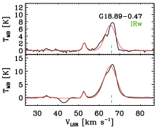
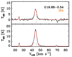
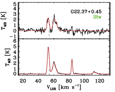
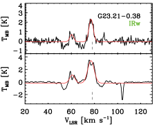
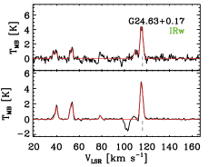
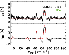
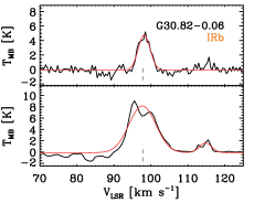
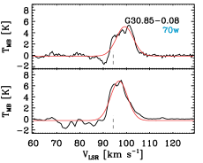
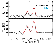
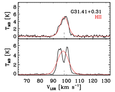
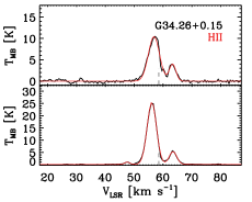
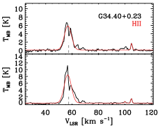
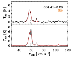
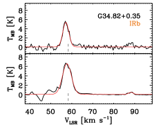
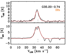
Figure 15: (continued)

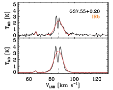
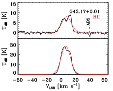
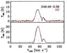
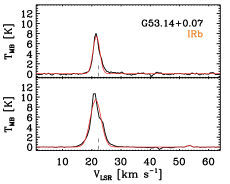
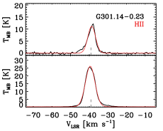
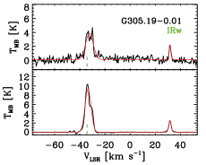
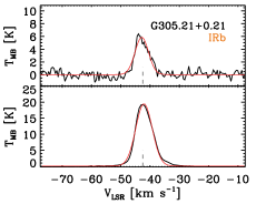
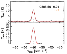
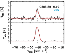
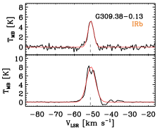
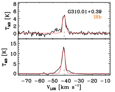
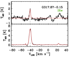
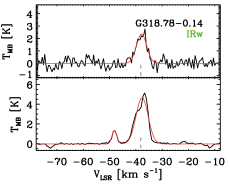
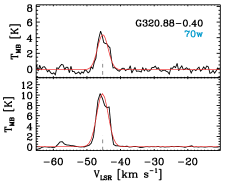
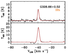
Figure 16: (continued)

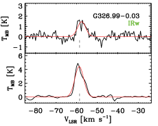
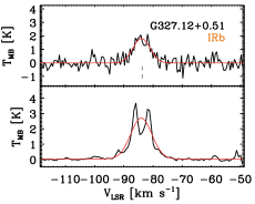
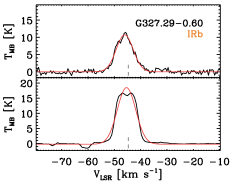
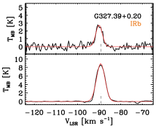
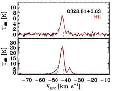
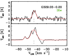
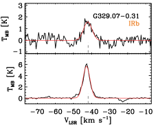
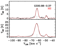
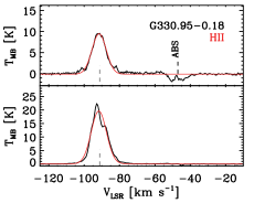
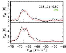
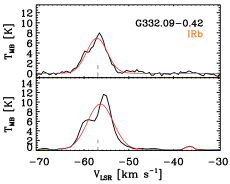
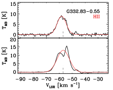
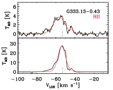
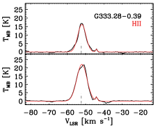
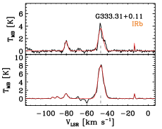
Figure 17: (continued)

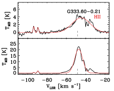
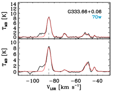
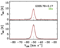
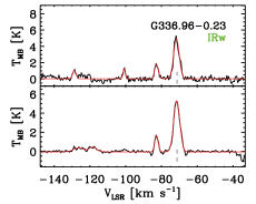
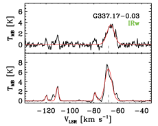
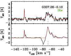
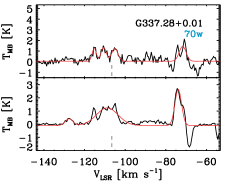
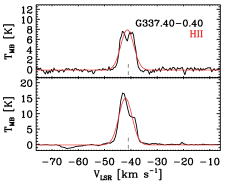
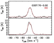
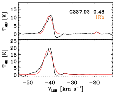
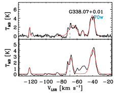
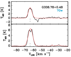
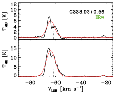
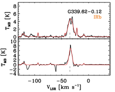
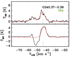
Figure 18: (continued)

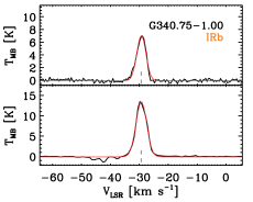
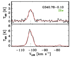
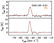
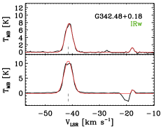
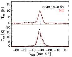
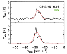
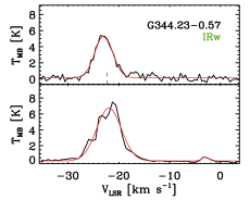
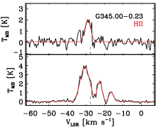
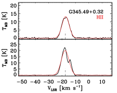
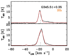
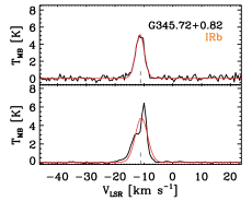
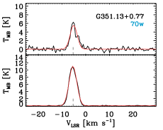
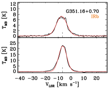
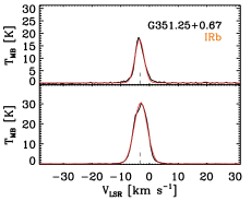
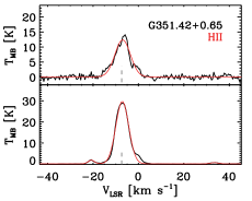
Figure 19: (continued)

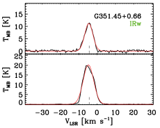
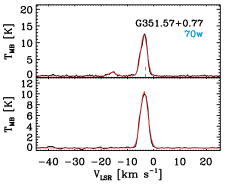
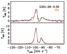
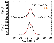
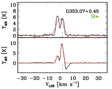
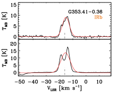
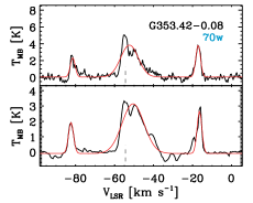
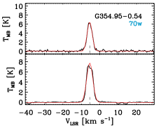
Figure 20: (continued)

Appendix C LTE calculation

To calculate the physical properties of the [C i]-traced main components (Sect. 5.1), we combined the APEX [C i] 492 GHz and 809 GHz observations and followed the LTE-based procedure as below. First, we started with the definition of optical depth:

$$\tau_{\varv}=\frac{c^{3}}{8\pi\nu^{3}}\left[\textrm{exp}\left(\frac{h\nu}{k_{\rm B}T_{\rm ex}}\right)-1\right]A_{\rm ul}\phi_{\varv}N_{\rm u}$$ (3)

where $c$ is the speed of light, $\nu$ is the frequency of the transition, $h$ is the Planck constant, $k_{\rm B}$ is the Boltzmann constant, $A_{\rm ul}$ is Einstein’s spontaneous emission coefficient, $\phi_{\varv}$ is the normalized spectral distribution of the transition as a function of velocity, and $N_{\rm u}$ is the column density of atoms in the upper transition state. With this definition of optical depth, the $\tau_{2-1}$-to-$\tau_{1-0}$ ratio can be written as

$$\frac{\tau_{2-1}}{\tau_{1-0}}=1.26\leavevmode\nobreak\ \textrm{exp}\left(\frac{-23.6}{T_{\rm ex}}\right)\frac{1-\textrm{exp}(-38.9/T_{\rm ex})}{1-\textrm{exp}(-23.6/T_{\rm ex})}$$ (4)

This equation assumes that [C i] 492 GHz and 809 GHz have the same excitation temperature and hence are in LTE. In addition, the atomic carbon column density can be estimated by

$$N(\textrm{C})=\frac{8\pi\nu^{3}}{c^{3}}\frac{Z}{A_{\rm ul}g_{\rm u}}\textrm{exp}\left(\frac{E_{\rm u}}{k_{\rm B}T_{\rm ex}}\right)\left[\textrm{exp}\left(\frac{h\nu}{k_{\rm B}T_{\rm ex}}\right)-1\right]^{-1}\int\tau_{\varv}\Delta\varv,$$ (5)

where $g_{\rm u}$ and $E_{\rm u}$ are the statistical weight and energy of the upper transition state. The partition function $Z$ is defined as

$$\begin{split}Z&=\sum_{i=0}^{2}g_{i}\leavevmode\nobreak\ \textrm{exp}\left(\frac{-E_{i}}{k_{\rm B}T_{\rm ex}}\right)\\ &=1+3\leavevmode\nobreak\ \textrm{exp}(-23.6/T_{\rm ex})+5\leavevmode\nobreak\ \textrm{exp}(-62.5/T_{\rm ex})\end{split}$$ (6)

On the other hand, we considered the brightness temperature emitted from a region of uniform excitation temperature:

$$T_{\rm B}=\frac{h\nu/k_{\rm B}}{\textrm{exp}(h\nu/k_{\rm B}T_{\rm ex})-1}\left[1-\textrm{exp}(-\tau)\right].$$ (7)

For [C i] 492 GHz and 809 GHz, $\tau_{1-0}$ and $\tau_{2-1}$ can be written as

$$\tau_{1-0}=-\textrm{ln}\left[1-T_{\rm B}(1-0)\frac{\textrm{exp}(23.6/T_{\rm ex})-1}{23.6}\right]$$ (8)

$$\tau_{2-1}=-\textrm{ln}\left[1-T_{\rm B}(2-1)\frac{\textrm{exp}(38.9/T_{\rm ex})-1}{38.9}\right].$$ (9)

Therefore, the $\tau_{2-1}$-to-$\tau_{1-0}$ ratio is

$$\frac{\tau_{2-1}}{\tau_{1-0}}=\frac{-\textrm{ln}\left[1-T_{\rm B}(2-1)\frac{\textrm{exp}(38.9/T_{\rm ex})-1}{38.9}\right]}{-\textrm{ln}\left[1-T_{\rm B}(1-0)\frac{\textrm{exp}(23.6/T_{\rm ex})-1}{23.6}\right]}.$$ (10)

Solving Eqs. (4) and (10) with the measured brightness temperatures numerically results in $T_{\rm ex}$, as well as $\tau_{1-0}$ and $\tau_{2-1}$.