Approximating Triangular Meshes by Implicit, Multi-Sided Surfaces

Abstract

The I-patch is a multi-sided surface representation, defined as a combination of implicit ribbon and bounding surfaces, whose pairwise intersections determine the natural boundaries of the patch. Our goal is to show how a collection of smoothly connected I-patches can be used to approximate triangular meshes. We start from a coarse, user-defined vertex graph which specifies an initial subdivision of the surface. Based on this, we create ribbons that tightly fit the mesh along its edges in both positional and tangential sense, then we optimize the free parameters of the patch to better approximate the interior. If the surfaces are not sufficiently accurate, the network needs to be refined; here we exploit that the I-patch construction naturally supports T-nodes. We also describe a normalization method that nicely approximates the Euclidean distance field, and can be efficiently evaluated. The capabilities and limitations of the approach are analyzed through several examples.

Ágoston Sipos¹ , Tamás Várady² , Péter Salvi³

¹Budapest University of Technology and Economics, asipos@edu.bme.hu

²Budapest University of Technology and Economics, varady@iit.bme.hu

³Budapest University of Technology and Economics, salvi@iit.bme.hu

Corresponding author: Ágoston Sipos, asipos@edu.bme.hu

Keywords: implicit surfaces, multi-sided patches, mesh approximation

DOI: https://doi.org/10.14733/cadaps.2022.aaa-bbb

1 INTRODUCTION

Implicit surfaces have many nice qualities. They are generally $C^{\infty}$-continuous and represent half-spaces, so point-membership classification is straightforward. No parameterization is needed for distance computations and approximating data points, and they are favorable for several geometric interrogations, such as ray tracing or surface intersections. Simple regular shapes (such as planes, cylinders, cones, etc.) are commonly represented by implicit surfaces. Free-form modeling, however, is more controversial. Counter-arguments include various shape problems, such as singularities, self-intersections, handling several disconnected surface portions, and the rigidity of the shapes using only limited shape parameters. In this paper we investigate how to approximate a triangular mesh by a collection of smoothly connected, multi-sided patches. We wish to preserve the benefits of the implicit representation and try to eliminate difficulties by retaining the patch within a well-defined subspace. We assume that the triangular mesh represents an object bounded by large free-form faces, without high curvature variations or tiny features. We also assume that there exists a coarse initial network associated with the mesh; its vertices determine the corners of the patches to be constructed, and its edges define loops for the patchwork. Such a network may be created by a user, produced by an automatic quad meshing algorithm, or defined by a 3D cell structure—examples will be given later. We compute an approximating patchwork and evaluate the deviations. If the accuracy is not sufficient, we adaptively refine the initial structure by subdivision (permitting T-nodes) and then refit as needed. Our representation of choice is the I-patch [21], a class of implicit surfaces that interpolate a loop of boundary curves. Each segment is defined as the intersection of a ribbon (primary surface) and a bounding surface, both given in implicit form, similarly to functional splines [10]. Thus the boundaries may be general 3D curves, or planar curves when either the ribbon or the bounding surface is represented by a plane. I-patches smoothly join to the given ribbons. In this paper we prescribe only $G^{1}$ connections, although the algebra permits higher-degree continuity, as well. The ribbons and bounding surfaces are determined in such a way that the I-patch interpolates corner points on the mesh and approximates underlying data points. I-patches have a few free scalar parameters, by means of which the interior can be efficiently optimized. The paper is structured in the following way. After briefly reviewing previous work in Section 2, we describe the basic equations of I-patches in Section 3. We introduce a faithful distance field for I-patches (Section 4) and then explain what sort of ribbon and bounding surfaces (Section 5) will be used for an optimized mesh approximation (Section 6). The concept of refining the curve network will be presented in Section 7, followed by a few examples to illustrate the capabilities and limitations of our approach (Section 8).

2 PREVIOUS WORK

There is a vast range of algorithms for creating implicit surfaces interpolating or approximating point data. These can be categorized into several classes, such as methods based on local approximations [6, 14], algebraic splines [7, 4], radial basis functions [2, 15], moving least squares [17], Poisson surface reconstruction [8], or even neural networks [19]. All of these methods are very general, and can be used on unorganized point sets. Because of this, they also share some common properties: the created function is a highly “algebraic” formulation, almost devoid of geometric meaning, and the resulting surface often has high-frequency variations. Our context is much more restricted: the input points are organized into a mesh, and additional structure is supplied by a user-defined vertex graph. These allow us to create a model by connecting relatively low-degree, high-quality single-patch surfaces composed of geometrically intelligible parts. In this sense, implicit modeling techniques are more relevant to this research, including the blending methods of Rockwood [16] and Warren [22], as well as A-patches [1] and functional splines [10, 5], although these were not used for approximation per se. In this work we investigate the approximation capabilities of I-patches [21]. This is a continuation of our former research, where we have shown how to construct I-patches for applications in polyhedral design and setback vertex blending. The I-patch representation is inherently multi-sided, with implicitly defined, but exact boundary curves and cross-derivative constraints. This sets it apart from the other blending methods outlined above—see our previous paper [18] for more information and some comparisons.

3 PRELIMINARIES: I-PATCHES

An $n$-sided I-patch is defined by $n$ ribbons and bounding surfaces, given in implicit form as $R_{i}(x,y,z)=0$ and $B_{i}(x,y,z)=0$, respectively ($i=1\dots n$), see Figure 1. The patch itself is constructed as the 0-isosurface of

$$I(x,y,z)=\sum_{i=1}^{n}w_{i}R_{i}(x,y,z)\prod_{j\neq i}B_{j}^{2}(x,y,z)-w_{0}\prod_{i=1}^{n}B_{i}^{2}(x,y,z),$$ (1)

where $w_{i}$ ($i=0\dots n$) are free scalar parameters. It is defined within the volume enclosed by the bounding surfaces, i.e., for points where $B_{i}(x,y,z)\geq 0$ for all $i$. (For readability, we will omit the $(x,y,z)$ arguments of all implicit surfaces from now on.) The intersection of $R_{i}$ and $B_{i}$ defines the $i$-th boundary curve, which is interpolated by the I-patch, since all terms of the above expression vanish there. Similarly, it is easy to show that at these points the gradient of $R_{i}$ will be parallel to the gradient of the I-patch, so $G^{1}$ continuity is ensured. (Raising the degrees in Eq. (1) would guarantee a higher order of continuity.) When two or more bounding surfaces coincide, special handling is needed [18]. Apart from points on the bounding surfaces, an equivalent formulation is given by the $w_{0}$-isosurface of

$$I_{w_{0}}=\sum_{i=1}^{n}\frac{w_{i}R_{i}}{B_{i}^{2}}=:\sum_{i=1}^{n}d_{i},$$ (2)

where each $d_{i}$ can be regarded as a distance measure associated with the $i$-th ribbon, so I-patches can be interpreted as the locus of 3D points where the sum of $n$ distances is constant. This is similar to the logic of how some classic surfaces, such as ellipsoids, are derived. We remark that an ellipsoid can in fact be exactly represented in the above rational form.

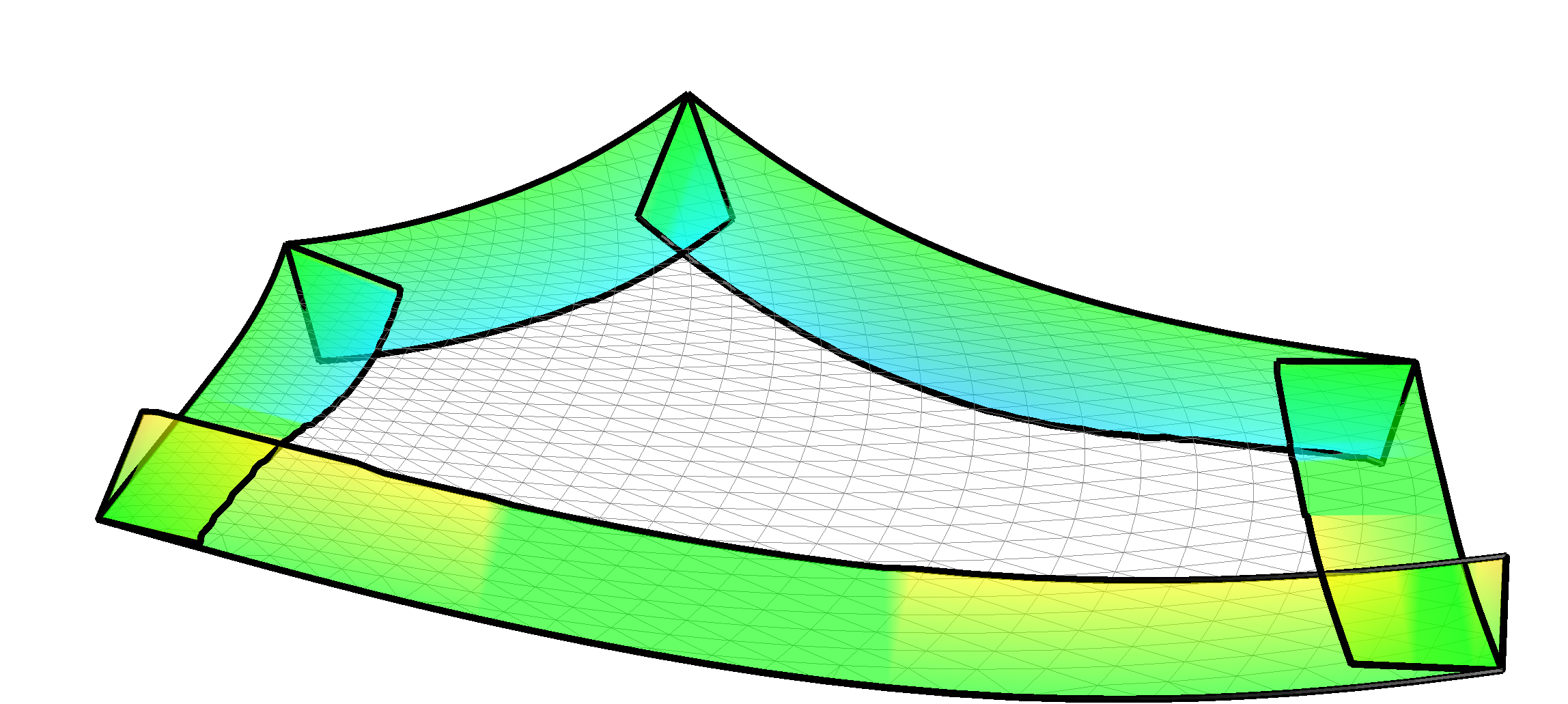
(a) Ribbons

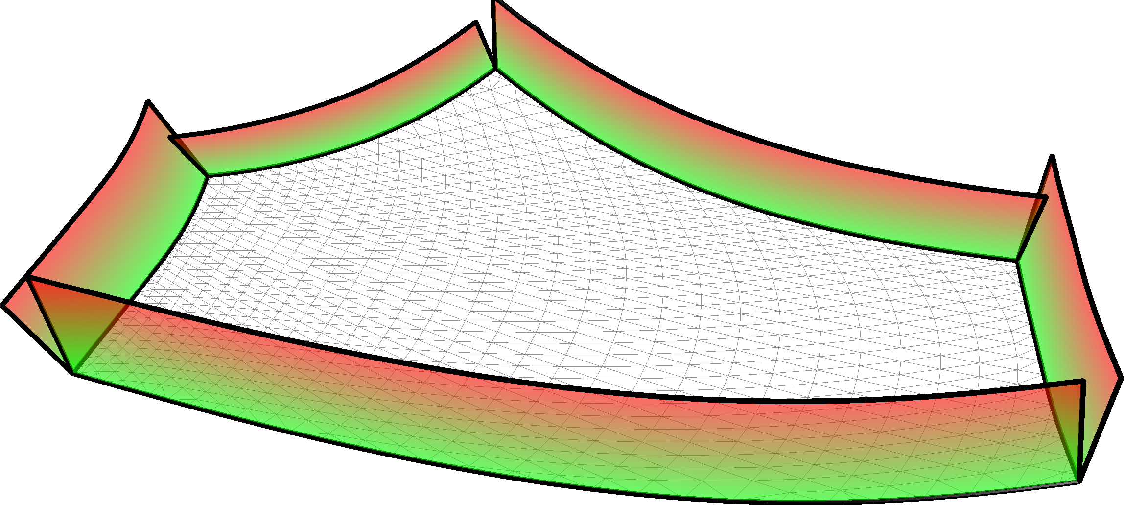
(b) Bounding surfaces

(c) I-patch

Figure 1: Construction of an I-patch.

4 FAITHFUL DISTANCE FIELD

The computation of distances from a given surface, or the creation of an offset surface by a given distance, are heavily used operations in several applications, such as design, geometric intersections and interrogations, and data approximation. One advantage of implicit surfaces is that they possess a natural distance field from their $0$-isosurfaces. Unfortunately algebraic distances, even when multiplied by a carefully chosen scalar factor, do not yield Euclidean distances, except for planes. A frequently applied, practical method for enhancing distance fields is to normalize the implicit equation by the norm of its gradient [20]. This is a good solution to obtain approximate Euclidean distances in the vicinity of the $0$-isosurface, but these expressions contain square roots, and may exhibit singularities. They also deviate from the correct distance when we move farther away from the implicit surface. We propose a normalization for I-patches that produces a good approximation of the Euclidean distance field, not only in the vicinity of the surface, but in a much wider range. The literature often uses the terminology “faithful” for such distances [12], and we also retain this adjective.

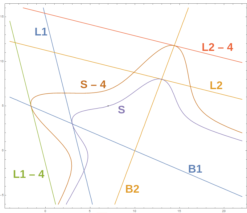
(a) Faithful normalization

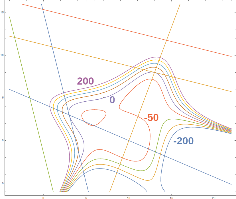
(b) No normalization

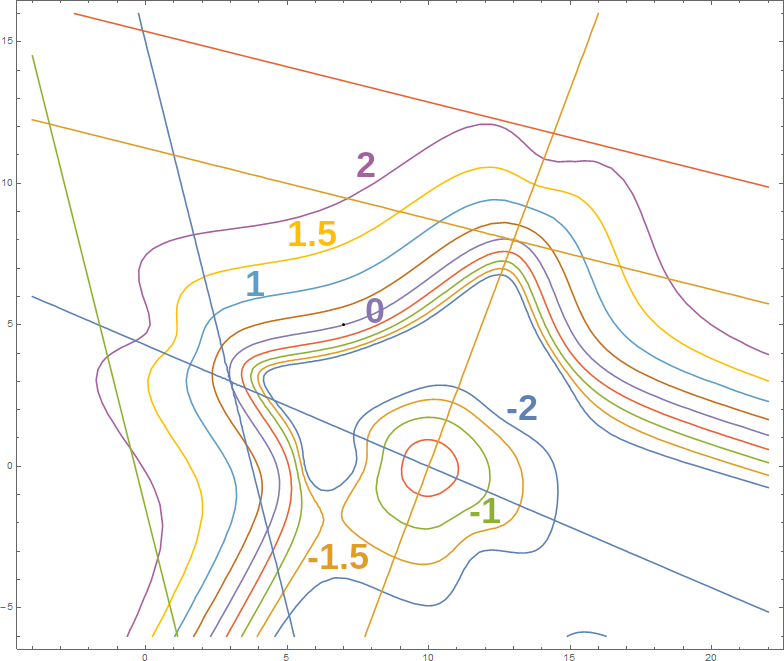
(c) Gradient normalization

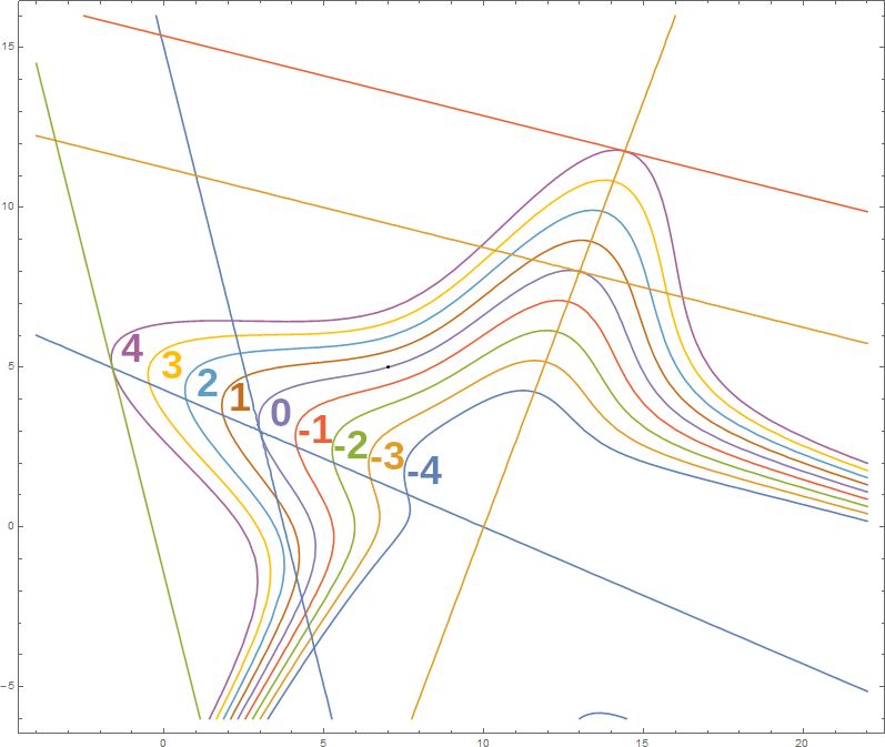
(d) Faithful normalization

Figure 2: Offsets of an I-segment using different normalizations.

Using the notation $\alpha_{i}=w_{i}/B_{i}^{2}$, we can formulate the equation of the I-patch as a weighted sum of ribbon surfaces $R_{i}$, multiplied by blending functions:

$$I=\sum_{i=1}^{n}R_{i}\cdot\alpha_{i}-w_{0}.$$ (3)

We derive a faithful normalization by dividing with the sum of the blending functions:

$$\hat{I}=\frac{\sum_{i=1}^{n}R_{i}\cdot\alpha_{i}-w_{0}}{\sum_{i=1}^{n}\alpha_{i}}.$$ (4)

Examining an algebraic offset of the normalized I-patch, we find that

$$\hat{I}-d=\frac{\sum_{i=1}^{n}(R_{i}-d)\cdot\alpha_{i}-w_{0}}{\sum_{i=1}^{n}\alpha_{i}}.$$ (5)

In other words, the offset of the normalized I-patch is also a normalized I-patch, created from ribbon offsets, and blended by the same $\alpha_{i}$ functions (i.e., the same bounding surfaces). The faithfulness of this formulation depends on the distance field of the ribbons. I-lofts (see Section 5), for example, can be made faithful in this sense, since they are defined by combining planar ribbons. As a consequence, an I-patch combining I-lofts will also behave in a faithful manner. First we demonstrate this concept in 2D using an I-segment $S$, which is a planar implicit curve, that blends together two lines $L_{1}$ and $L_{2}$ (Fig. 2(a)). We wish to compute an offset of the I-segment that smoothly connects the accurately displaced offset lines $L_{1}-d$ and $L_{2}-d$, and expect to obtain a good distance field between them. Figure 2(b) shows the distribution of algebraic distances, and Figure 2(c) shows the distance field after gradient normalization, where one can observe the uneven and unproportional distribution of the offset curves. Our proposed normalization in Figure 2(d) shows a faithful distance field. Faithful distances are important in our context. Offsets of I-patches or I-segments can be directly computed yielding good approximations of Euclidean distances. Approximating data points using I-patches or I-lofts becomes easy and computationally efficient, since we only need to substitute into the above normalized equations, and optimize accordingly. In Figure 3 an I-patch is shown with its offset, using mean curvature maps. Figures 3(a) and 3(b) show the patch and its offset isosurface, and Figure 4 shows four superimposed offset patches with $d=-5$, $0$, $5$ and $10$.

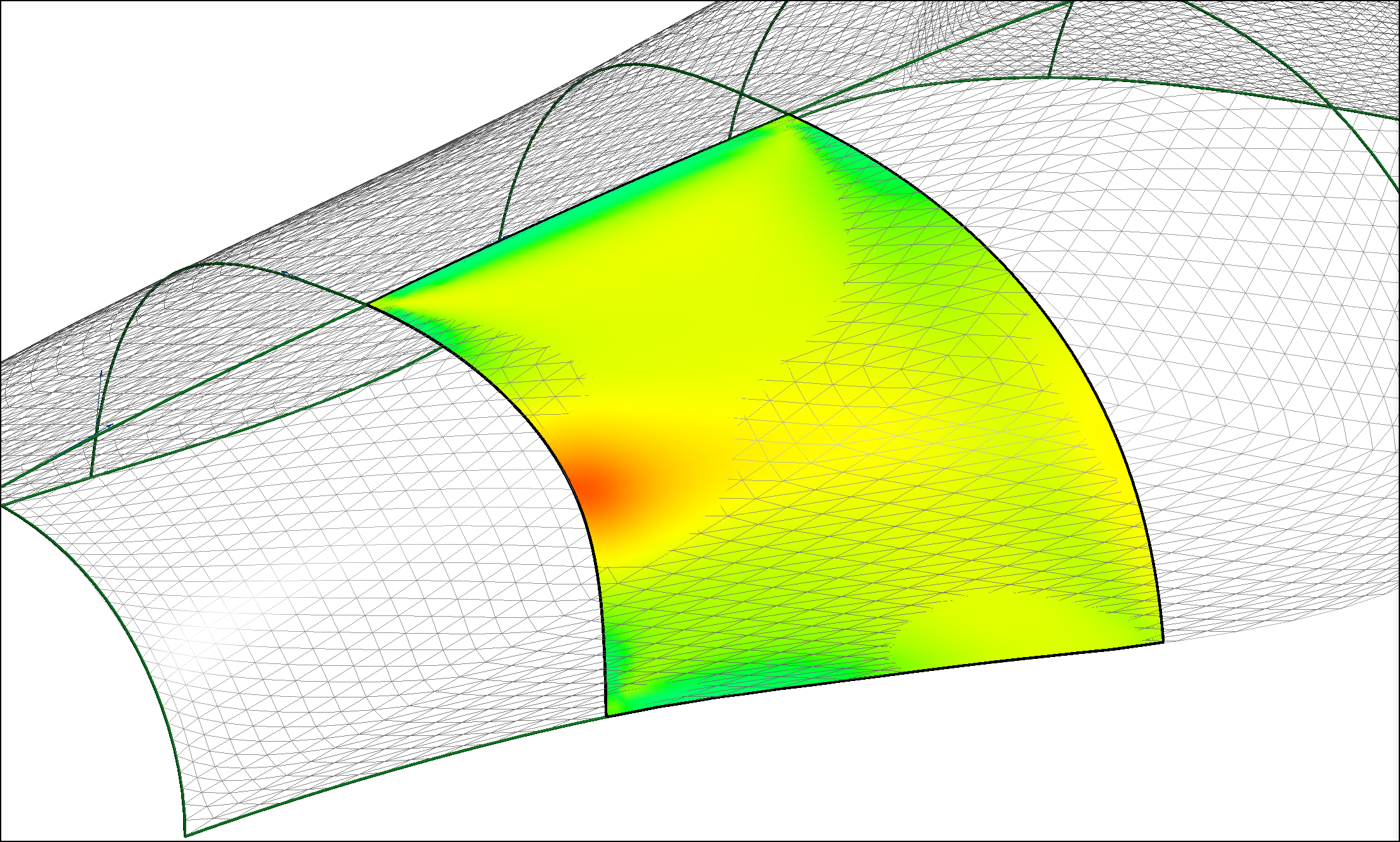
(a) Original surface

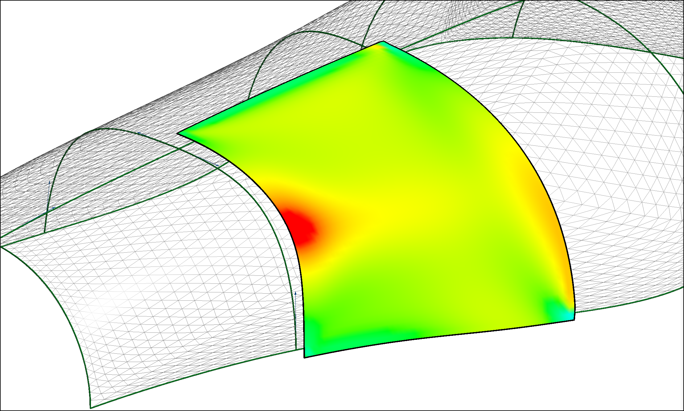
(b) Offset surface

Figure 3: Offsetting an I-patch.

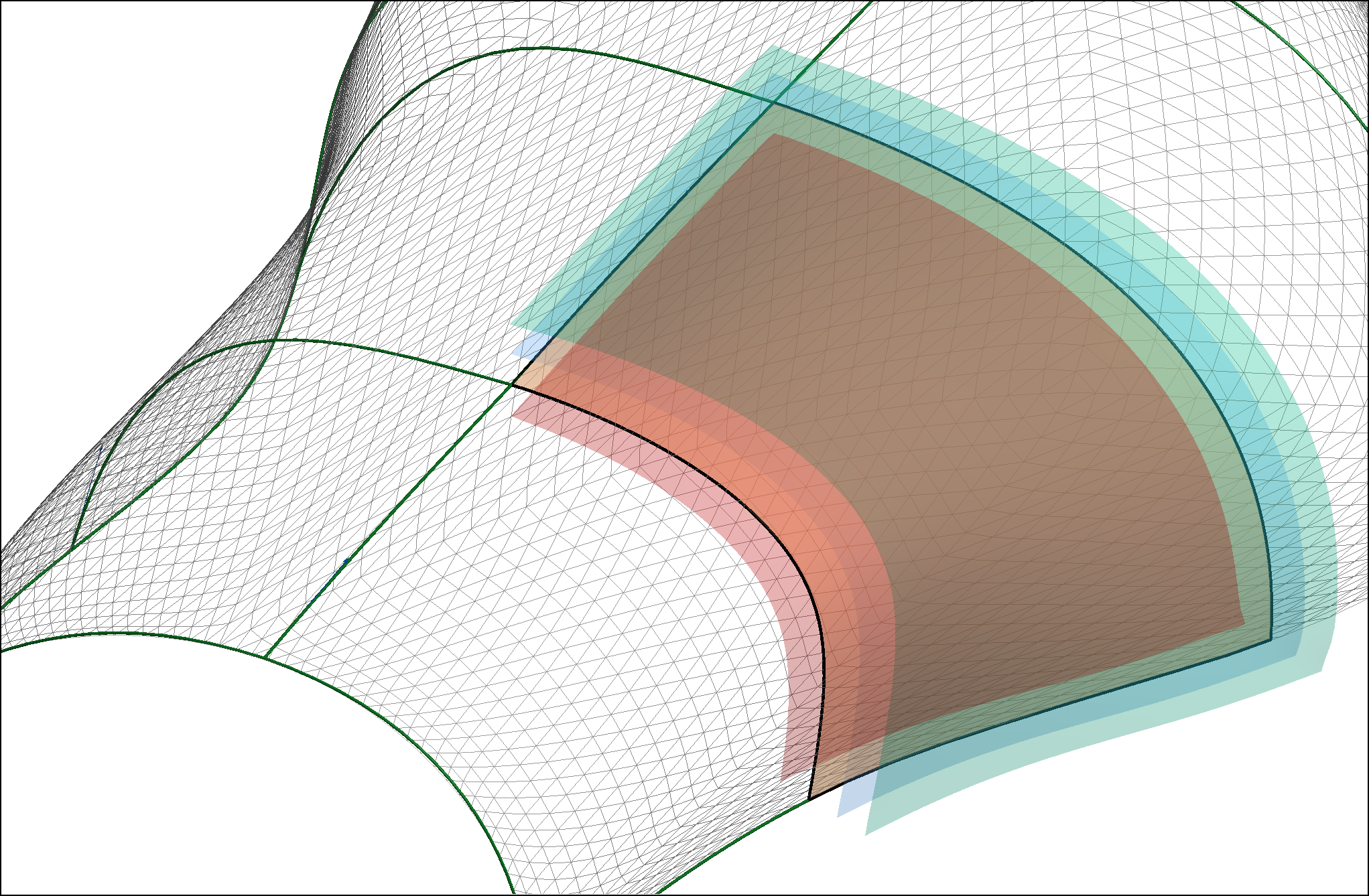
Figure 4: Multiple offsets of an I-patch.

Finally, note that the same principle works with the polynomial form of the I-patch:

$$\hat{I}=\frac{\sum_{i=1}^{n}w_{i}R_{i}\prod_{j\neq i}B_{j}^{2}-w_{0}\prod_{i=1}^{n}B_{i}^{2}}{\sum_{i=1}^{n}w_{i}\prod_{j\neq i}B_{j}^{2}}.$$ (6)

This is a more complex, but equivalent equation, which can be evaluated on the boundary, as well.

5 RIBBONS AND BOUNDING SURFACES

In this section we introduce the ribbons and bounding surfaces needed for the current I-patch construction. As will be explained below, these surfaces are always defined as weighted combinations of planes given at the corner points and auxiliary planes derived from the corner data. Let us take two adjacent corner points $\mathbf{p}_{1}$, $\mathbf{p}_{2}$, and incident corner planes $\pi_{1}$, $\pi_{2}$ with normal vectors $\mathbf{n}_{1}$, $\mathbf{n}_{2}$. The corresponding ribbon interpolates both points and normal vectors. Similarly, the bounding surface interpolates both points, but it is transversal to the ribbon surface. The ribbons and bounding surfaces are described by three kinds of equations: (i) planes, (ii) Liming-surfaces, and (iii) I-lofts. Liming [11] created conic curves as a combination of three implicitly given lines. A Liming-surface, in turn, is the combination of three planes given in implicit form. In addition to the corner planes $\pi_{i}$, an auxiliary cutting plane $\tilde{\pi}$ is needed that contains both $\mathbf{p}_{1}$ and $\mathbf{p}_{2}$ (see Fig. 5(a)). The surface equation is given as

$$(1-\lambda)\pi_{1}\pi_{2}-\lambda\tilde{\pi}^{2}=0,$$ (7)

where $\lambda$ controls the fullness. The choice of the cutting plane $\tilde{\pi}$ does affect the shape of the Liming-surface. Nevertheless, the simplest setting of its normal vector $\mathbf{n}_{12}=(\mathbf{n}_{1}+\mathbf{n}_{2})/2$ proved to be satisfactory. The parameter $\lambda$ is going to be defined by the optimal approximation of the underlying polyline boundary, see the next section.

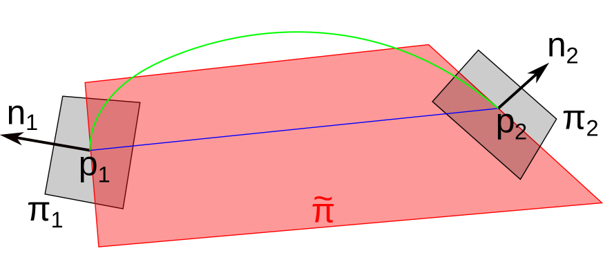
(a) Liming ribbon

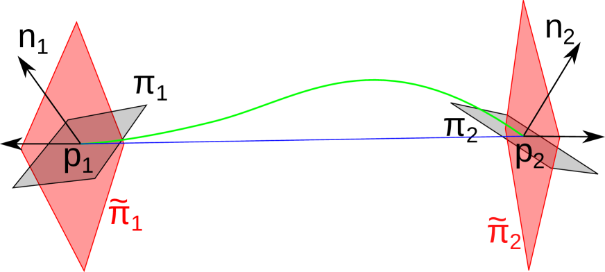
(b) I-loft ribbon

Figure 5: Constructing ribbons.

I-lofts are simple, two-sided I-patches defined by two pairs of planes containing the corner points. In this case primary ribbons correspond to the tangent planes at the corners ($\pi_{i}$), and the local bounding planes $\tilde{\pi}_{i}$ are transversal to these (see Fig. 5(b)). The equation of the I-loft is

$$w_{1}\pi_{1}\tilde{\pi}_{2}^{2}+w_{2}\pi_{2}\tilde{\pi}_{1}^{2}-\tilde{\pi}_{1}^{2}\tilde{\pi}_{2}^{2}=0.$$ (8)

There is freedom to select the bounding planes, as will be explained below. The weights $w_{1}$ and $w_{2}$ are shape parameters to set the fullness of I-lofts, and thus ensure the best approximation of the underlying polyline boundary, see the next section. In our context we prefer to use planar bounding surfaces to subdivide the interior of the mesh, since these lead to planar boundary curves, and the equation of the I-patch becomes simpler. Intersections with Liming ribbons yield conic curves, while we get planar I-segments with I-lofts. One simple formula to set the normal of this bounding plane comes from averaging the corner normals:

$$\mathbf{n}_{B}=\mathbf{n}_{12}\times(\mathbf{p}_{2}-\mathbf{p}_{1})\text{, where }\mathbf{n}_{12}=\frac{\mathbf{n}_{1}+\mathbf{n}_{2}}{2}.$$ (9)

Alternatively, we may rotate the bounding plane around the chord $\mathbf{p}_{2}-\mathbf{p}_{1}$, and may set it to contain a prescribed mesh point. It is a natural assumption that an optimal ribbon normal at the midpoint of the boundary curve should approximate the normal vector of the mesh. Curved bounding surfaces may be used in the interior of the mesh to approximate non-planar subdividing curves, but they must be used for the approximation of curved external boundaries. In this case, we calculate the local direction of the mesh boundary at the corner points; the tangent planes of the bounding surface are defined by this vector and the corresponding mesh normal. When a curved bounding surface is intersected with a curved ribbon, a general 3D curve is obtained. It should be noted, that although we always attempt to use the simplest ribbon–bounding surface pair, the use of Liming-surfaces is not always possible. If the boundary to be approximated has a point of inflection, or the corner normals are twisted, only I-lofts can be used [18]. It is also important to observe that the ribbons and the bounding surfaces depend only on the corner points, the corner normals and the mesh, so if two adjacent I-patches share the same $\mathbf{p}_{1}\mathbf{p}_{2}$ boundary, the identical surface components will guarantee a smooth connection.

6 I-PATCHES TO APPROXIMATE MESHES

In this section we describe how to construct I-patches that approximate a given mesh. At this point we assume that the bounding surfaces have already been determined. We intersect these with the mesh, and trace polylines between the adjacent corner points. We do not need tracing along the external edges of the mesh, since there the polylines are directly available. First we create ribbons that approximate these polylines, then an I-patch that approximates the interior points of the mesh. Ribbons match the given corner points and the corresponding normals (approximated from the mesh with standard methods [13, 3]). We construct a Liming-ribbon by optimizing its free $\lambda$ parameter. This sets the fullness of the ribbon, and determines the best approximating conic boundary. I-lofts are somewhat more flexible, and we have two independent scalar weights for the optimization. The error function to be minimized is the squared sum of the faithful algebraic distances (see Section 4). As mentioned earlier, it may be possible that a boundary can be approximated by both a Liming-surface and an I-loft. In this case, we choose the one with smaller error. Figure 6 shows a Liming and an I-loft ribbon, with corner planes and sampled points on the mesh. The deviation map indicates that the ribbons are close to the mesh (green) in the vicinity of the related boundary.

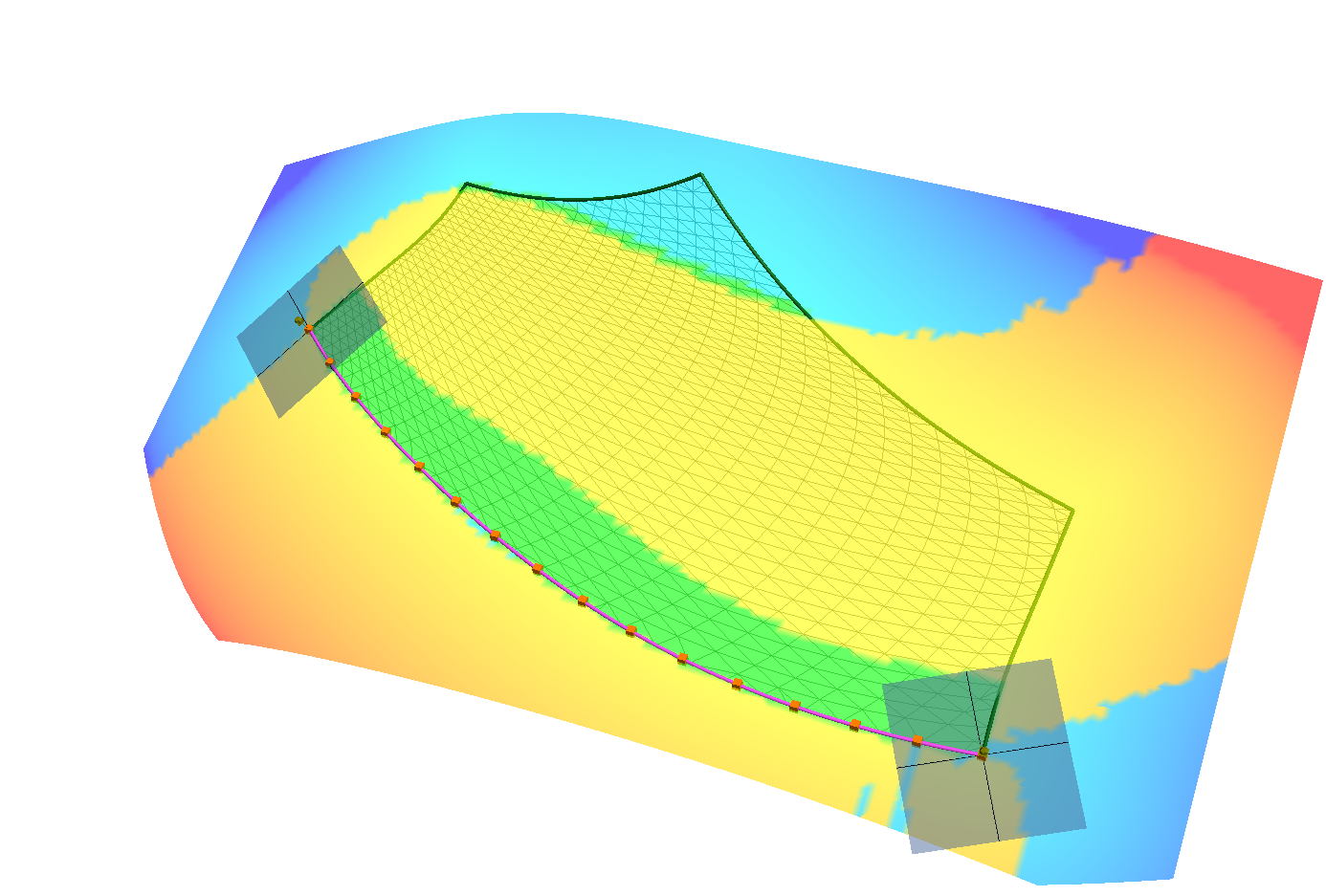
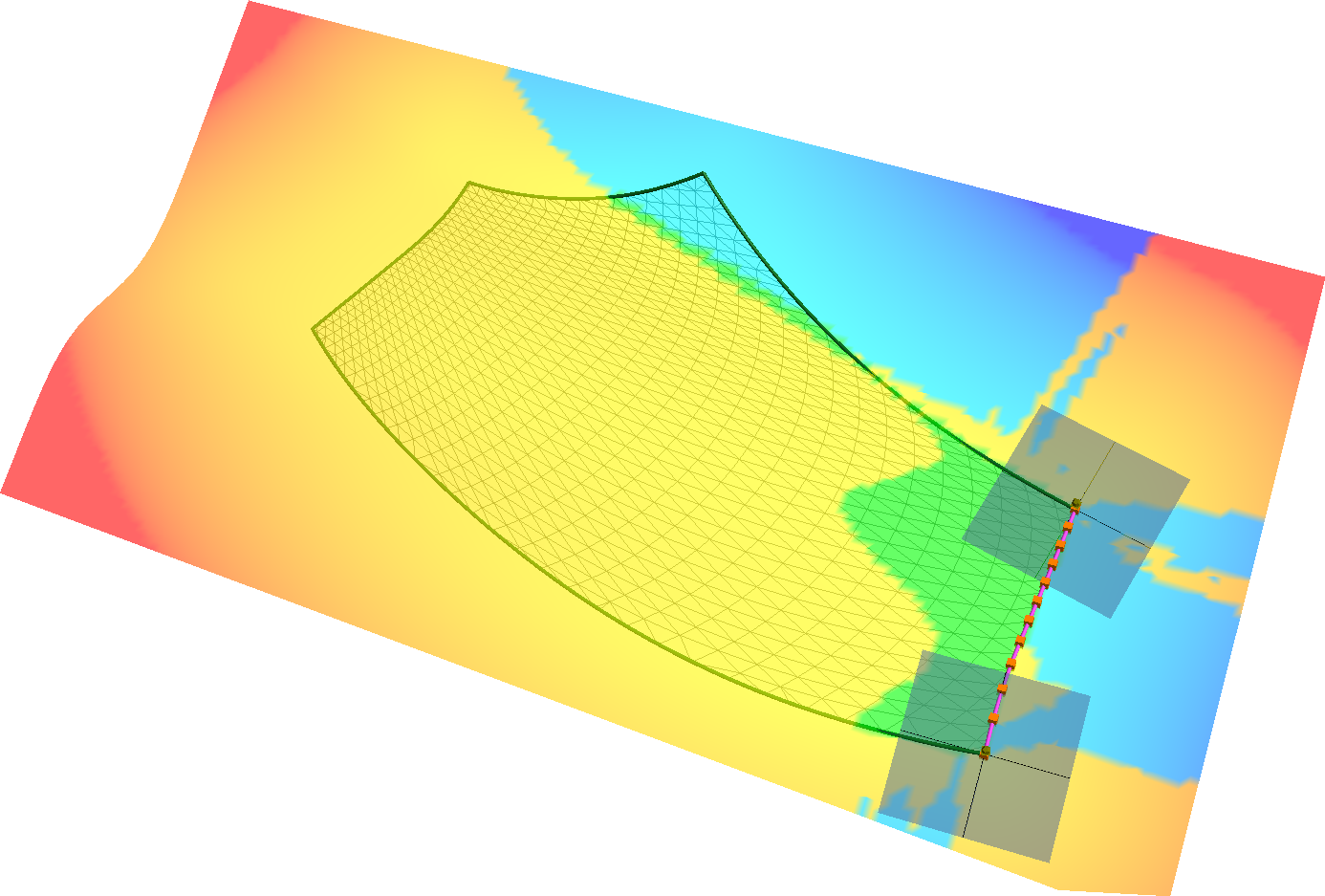
Figure 6: A Liming (left) and an I-loft ribbon (right), showing deviation from the mesh.

Next, mesh points are filtered out so only those remain that are enclosed by the bounding surfaces. Then we compute the mass center of the polyline boundaries of the patch, and project this point onto the mesh. This initial center point $\mathbf{c}$ is used to determine the default weights $w_{i}$ for the ribbons by enforcing that all terms $w_{i}/B^{2}_{i}(\mathbf{c}),i=1,..,n$ are equal. In other words, the default patch is composed in a way that the individual ribbons contribute to the patch in a uniform manner at the center point; the patch is also constrained to interpolate point $\mathbf{c}$. This initial setting can be iteratively improved to obtain the best approximation of the underlying data. We minimize the squared sum of the faithful distances, and set the optimal weights accordingly. For both the ribbon and patch optimization, derivative-free methods can be applied; we have chosen the Nelder–Mead algorithm [9]. We have observed that it is a good idea to limit the ratios of the optimized weights. Otherwise one ribbon may dominate the patch equation, and corrupt the surface quality along the other borders. Accordingly, we constrained how much the weights of the optimized ribbons can deviate from their initial values. This maximum ratio is a user parameter $\omega$. (In our examples, $\omega$ was set to $5$.) The formalized optimization problem is:

$$\operatorname*{arg\,min}_{\mathbf{w}}\sum_{i=1}^{N}I_{\mathbf{w}}(\mathbf{q}_{i}),\text{ s.t. }\max_{i,j}\left(\frac{w_{i}R_{i}(\mathbf{c})}{B_{i}^{2}(\mathbf{c})}\bigg{/}\frac{w_{j}R_{j}(\mathbf{c})}{B_{j}^{2}(\mathbf{c})}\right)\leq\omega,$$ (10)

where $\mathbf{w}=\{w_{i}\}_{1}^{n}$ is the vector of weights, and $\mathbf{q}_{i}$ ($i=1\dots N$) denotes the data points to be approximated. Figure 7(a) shows the curvature map of the optimized I-patch from Figure 1(c). We have assigned colors to the individual sides, and show the strength of the normalized blending functions in Figure 7(b).

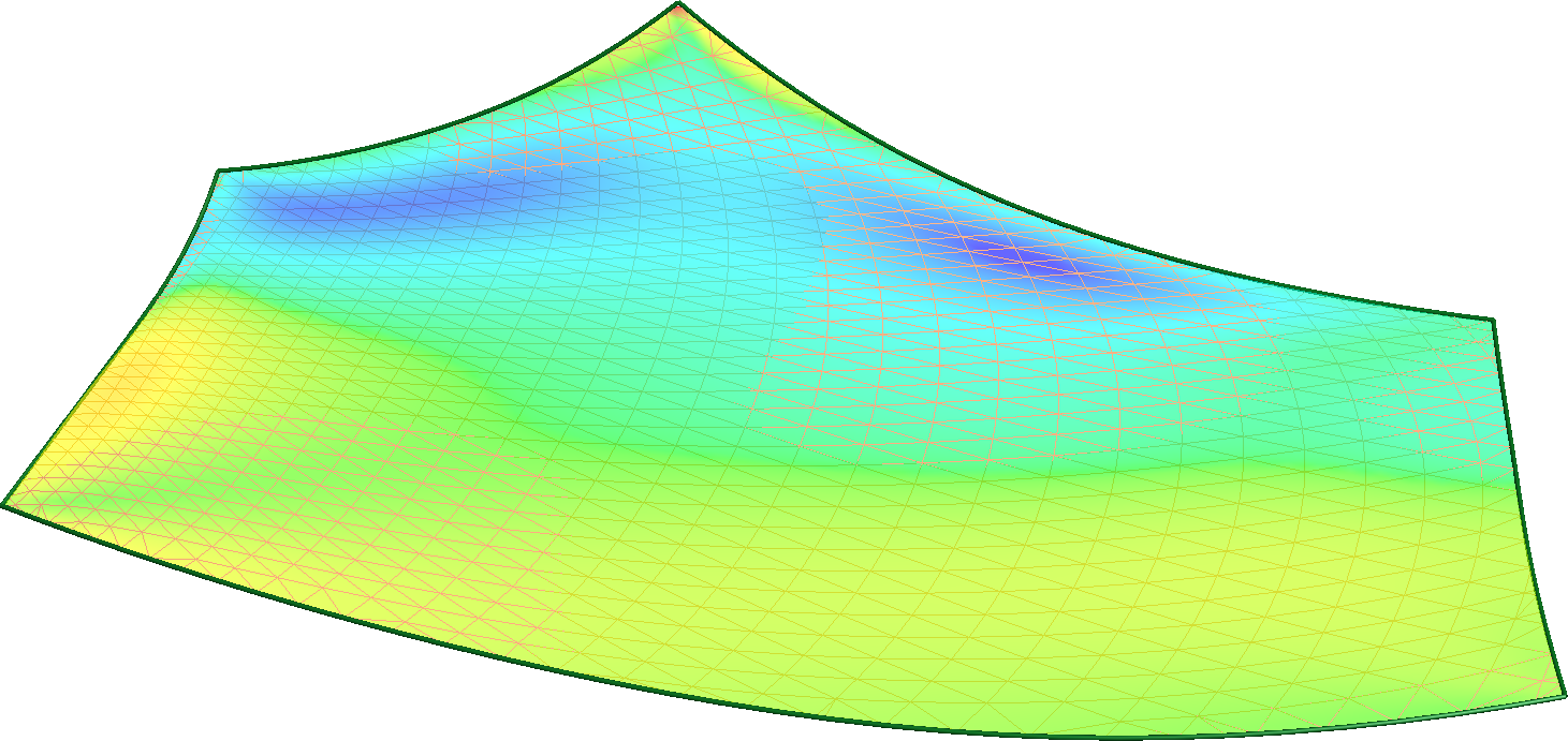
(a) Mean curvature map

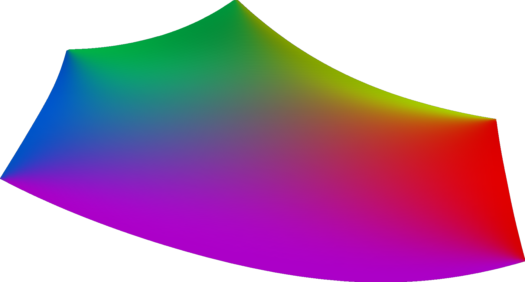
(b) Contributions of each side

Figure 7: Optimization of a 5-sided patch.

7 ADAPTIVE REFINEMENT OF THE PATCHWORK

Once an initial patchwork has been generated, we check whether it approximates the data points within a prescribed tolerance and—if necessary—we perform an adaptive refinement following simple heuristic rules. If a boundary is out of tolerance, it will be subdivided halfway between its endpoints. If a patch is out of tolerance, central splitting will be applied and a new mesh point will be inserted in its interior. We connect the new subdivision points, and add new artificial points in order to create a consistent structure. This leads to a new graph of edges with new ribbons and bounding surfaces, given in the same form as before, i.e., segments defined by two endpoints with normals, and an underlying polyline to be approximated. The above procedure automatically iterates until the requested accuracy is achieved. We remark that the initial network affects the structure of the final patchwork.

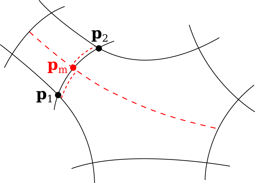
(a) X-node

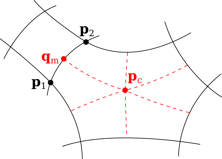
(b) T-node

Figure 8: Cases of adaptive refinement.

It is crucial, of course, to prevent the propagation of local refinements over the full patchwork, and subdivide only where it is necessary. Fortunately, I-patches are well-suited for producing T-nodes, as will be explained below. Figure 8(a) shows a boundary connecting $\mathbf{p}_{1}$ and $\mathbf{p}_{2}$ that needs to be subdivided; a new mesh point $\mathbf{p}_{m}$ is inserted, and four new boundaries are created. This is an X-node, where we compute a new position, and a new normal vector is taken from the mesh. Figure 8(b) shows another configuration, where the 6-sided patch needs to be centrally split at $\mathbf{p}_{c}$, which is the formerly described center point of the original patch. Here we wish to preserve the left ribbon connecting $\mathbf{p}_{1}$ and $\mathbf{p}_{2}$, and let the two adjacent subpatches of the subdivided patch inherit its midpoint $\mathbf{q}_{m}$ and the corresponding normal vector. In other words, the original ribbon and bounding surface is transferred, and $G^{1}$ continuity is naturally maintained. A related example will be shown in the next section.

8 EXAMPLES

Our first example in Figure 9 illustrates that I-patches naturally extend beyond the subspace determined by the bounding surfaces. Here we rendered the curvature map of the patch from Figure 3(a) using marching cubes.

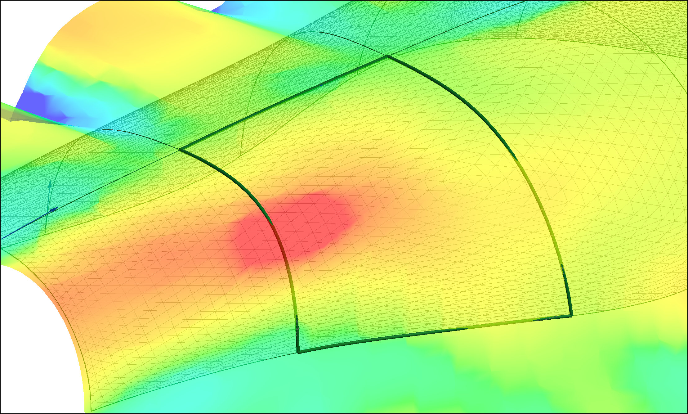
Figure 9: Natural extension of an I-patch.

The second example in Figure 10 shows the deviation map of a shoe last model. The network was created by a uniform cell structure yielding two 3-sided, six 4-sided and two 5-sided I-patches. The accuracy of the approximation—here and at the forthcoming pictures—will be measured in percentages relative to the diagonal of the bounding box. The average (Euclidean) deviation from the mesh is 0.069%, while the maximum is 0.35%.

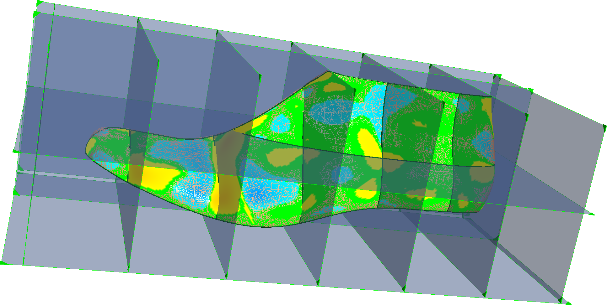
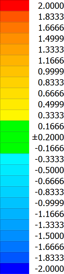
Figure 10: Cell-based subdivision on a model of a shoe last. The color legend shows absolute deviation values; the bounding box diagonal is 410 units long.

The third example (Fig. 11) is a sheet metal part composed of six 4-sided and two 5-sided patches, illustrating the effect of optimization and refinement. Figures 11(a) and 11(b) show two deviation maps, without and with optimization. Accuracies improve, as shown in Table 1.

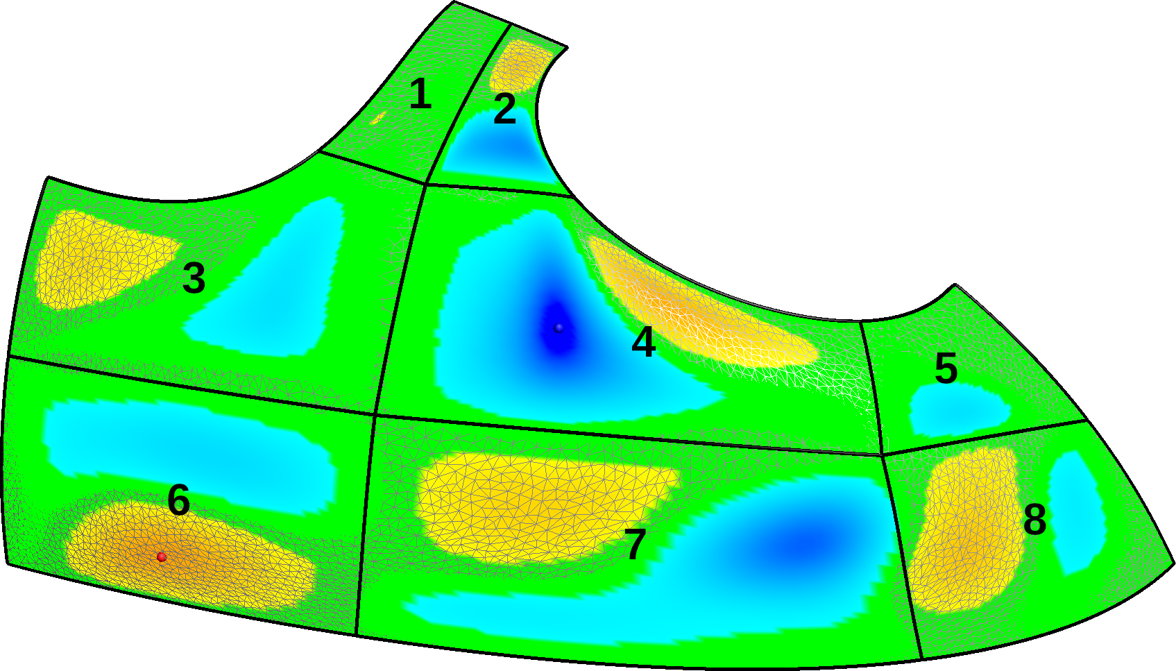
(a) Original surface w/o optimization

(b) Original surface with optimization

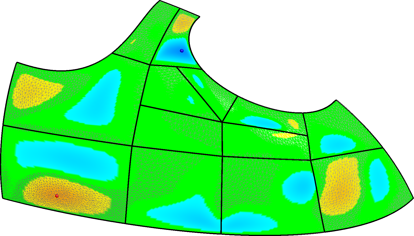
(c) Subdivided surface w/o optimization

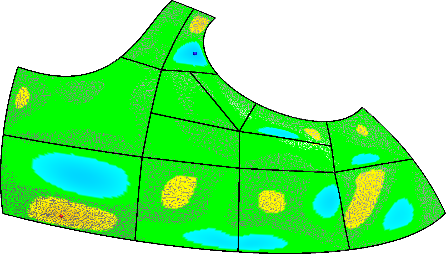
(d) Subdivided surface with optimization

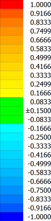
Figure 11: Subdivision of a sheet metal part, with T-nodes and a split. The color legend shows absolute deviation values; the bounding box diagonal is 270 units long.

Figures 11(c) and 11(d) show the deviation map of a refined structure—patch #4 and patch #7 have been subdivided. As both of these patches are inaccurate, their boundary is subdivided, and a new X-node is inserted. Boundaries 2–4, 3–4 and 4–5 are sufficiently accurate, so we retain and inherit the ribbons from patches #2, #3 and #5, and create T-nodes accordingly, when patch #4 is subdivided by a central split. For simplicity’s sake, planar bounding surfaces were generated throughout this refinement. The refined structure is more accurate, and it can be further improved by optimization (see Table 1). Finally, Figure 12 shows the front part of a concept car. The first image depicts the initial ribbons of a sparse network that has been refined in two steps. The deviations decrease as the number of I-patches increases, see Table 2.

Model	Average deviation	Maximum deviation
Original w/o optimization (Fig. 11(a))	0.055%	0.399%
Original with optimization (Fig. 11(b))	0.035%	0.226%
Split w/o optimization (Fig. 11(c))	0.041%	0.283%
Split with optimization (Fig. 11(d))	0.029%	0.175%

Table 1: Quantitative results corresponding to Figure 11.

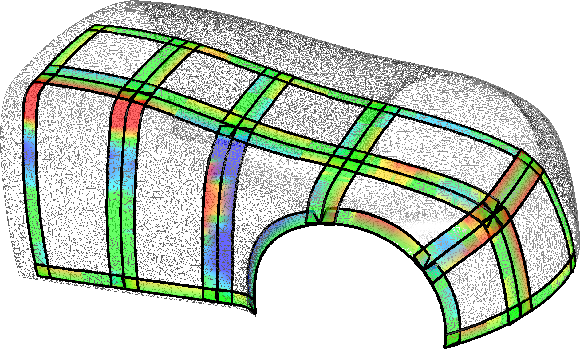
(a) Initial ribbons

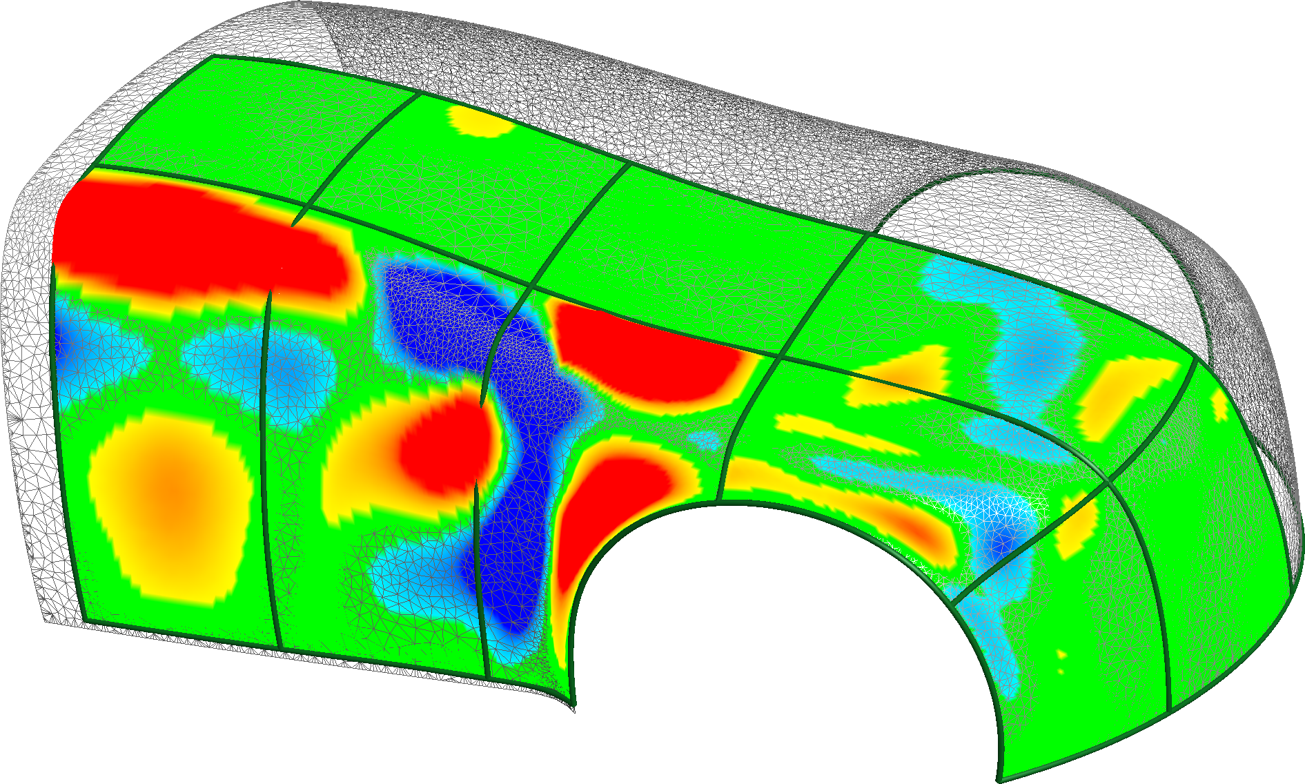
(b) Initial patchwork

(c) First refinement step

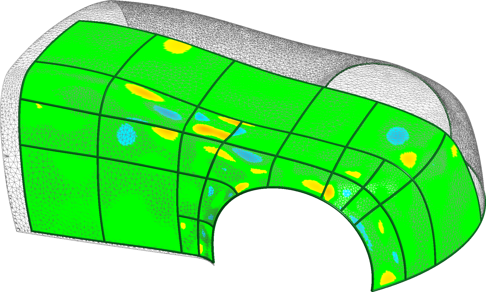
(d) Second refinement step

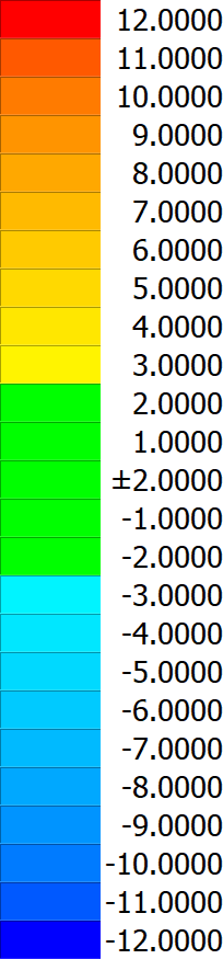
Figure 12: Steps of adaptive refinement on a concept car model. The color legend shows absolute deviation values; the bounding box diagonal is 4400 units long.

9 CONCLUSIONS

We have shown that it is possible to approximate a free-form object by a patchwork of smoothly connected, multi-sided implicit patches, defined by corner points placed on a mesh, and a graph that determines the connectivity between them. We have used a special class of I-patches, constructed from implicit ribbon and bounding surfaces determined solely by planes extracted from the mesh. The patches are optimized by various fullness weights in a computationally efficient manner, due to a faithful distance field that well approximates Euclidean distances. Clearly, I-patches represent a more rigid variety of shapes than their parametric counterparts, but nevertheless they have several interesting geometric and computational properties. Concerning future topics—we have used simple rules for defining the ribbon and bounding surfaces, leaving many other options to be explored in order to obtain better shapes and more complex patch boundaries. We also consider determining the best possible approximations for parametric patches. Efficient visualization of I-patches using GPUs is also an interesting problem.

REFERENCES

REFERENCES

- [1] Bajaj, C.L.; Chen, J.; Xu, G.: Modeling with cubic A-patches. ACM Transactions on Graphics (TOG), 14(2), 103–133, 1995. http://doi.org/10.1145/221659.221662.
- [2] Carr, J.C.; Beatson, R.K.; Cherrie, J.B.; Mitchell, T.J.; Fright, W.R.; McCallum, B.C.; Evans, T.R.: Reconstruction and representation of 3D objects with radial basis functions. In Proceedings of the 28th Annual Conference on Computer Graphics and Interactive Techniques, 67–76, 2001. http://doi.org/10.1145/383259.383266.
- [3] Cazals, F.; Pouget, M.: Estimating differential quantities using polynomial fitting of osculating jets. Computer Aided Geometric Design, 22(2), 121–146, 2005. http://doi.org/10.1016/j.cagd.2004.09.004.
- [4] Hamza, Y.F.; Lin, H.; Li, Z.: Implicit progressive-iterative approximation for curve and surface reconstruction. Computer Aided Geometric Design, 77, 101817, 2020. http://doi.org/10.1016/j.cagd.2020.101817.
- [5] Hartmann, E.: Implicit -blending of vertices. Computer Aided Geometric Design, 18(3), 267–285, 2001. http://doi.org/10.1016/S0167-8396(01)00030-9.
- [6] Hoppe, H.; DeRose, T.; Duchamp, T.; McDonald, J.; Stuetzle, W.: Surface reconstruction from unorganized points. In Proceedings of the 19th Annual Conference on Computer Graphics and Interactive Techniques, 71–78, 1992. http://doi.org/10.1145/133994.134011.
- [7] Jüttler, B.; Felis, A.: Least-squares fitting of algebraic spline surfaces. Advances in Computational Mathematics, 17(1), 135–152, 2002. http://doi.org/10.1023/A:1015200504295.
- [8] Kazhdan, M.; Hoppe, H.: Screened Poisson surface reconstruction. ACM Transactions on Graphics (TOG), 32(3), 1–13, 2013. http://doi.org/10.1145/2487228.2487237.
- [9] Kochenderfer, M.J.; Wheeler, T.A.: Algorithms for Optimization. MIT Press, 2019. ISBN 978-0-26-203942-0.
- [10] Li, J.; Hoschek, J.; Hartmann, E.: -functional splines for interpolation and approximation of curves, surfaces and solids. Computer Aided Geometric Design, 7(1–4), 209–220, 1990. http://doi.org/10.1016/0167-8396(90)90032-m.
- [11] Liming, R.A.: Conic lofting of streamline bodies: the basic theory of a phase of analytic geometry applicable to aircraft. Aircraft Engineering and Aerospace Technology, 19(7), 222–228, 1947. http://doi.org/10.1108/eb031528.
- [12] Lukács, G.; Martin, R.; Marshall, D.: Faithful least-squares fitting of spheres, cylinders, cones and tori for reliable segmentation. In European Conference on Computer Vision, 671–686, 1998. http://doi.org/10.1007/BFb0055697.
- [13] Max, N.: Weights for computing vertex normals from facet normals. Journal of Graphics Tools, 4(2), 1–6, 1999. http://doi.org/10.1080/10867651.1999.10487501.
- [14] Ohtake, Y.; Belyaev, A.; Alexa, M.; Turk, G.; Seidel, H.P.: Multi-level partition of unity implicits. In ACM SIGGRAPH 2005 Courses, 173–es. ACM, 2005. http://doi.org/10.1145/1198555.1198649.
- [15] Ohtake, Y.; Belyaev, A.; Seidel, H.P.: A multi-scale approach to 3D scattered data interpolation with compactly supported basis functions. In 2003 Shape Modeling International, 153–161, 2003. http://doi.org/10.1109/SMI.2003.1199611.
- [16] Rockwood, A.P.: The displacement method for implicit blending surfaces in solid models. ACM Transactions on Graphics (TOG), 8(4), 279–297, 1989. http://doi.org/10.1145/77269.77271.
- [17] Shen, C.; O’Brien, J.F.; Shewchuk, J.R.: Interpolating and approximating implicit surfaces from polygon soup. In ACM SIGGRAPH 2004 Papers, 896–904. ACM, 2004. http://doi.org/10.1145/1186562.1015816.
- [18] Sipos, Á.; Várady, T.; Salvi, P.; Vaitkus, M.: Multi-sided implicit surfacing with I-patches. Computers & Graphics, 90, 29–42, 2020. http://doi.org/10.1016/j.cag.2020.05.009.
- [19] Takikawa, T.; Litalien, J.; Yin, K.; Kreis, K.; Loop, C.; Nowrouzezahrai, D.; Jacobson, A.; McGuire, M.; Fidler, S.: Neural geometric level of detail: Real-time rendering with implicit 3D shapes. arXiv preprint arXiv:2101.10994, 2021. https://arxiv.org/abs/2101.10994.
- [20] Taubin, G.: Distance approximations for rasterizing implicit curves. ACM Transactions on Graphics (TOG), 13(1), 3–42, 1994. http://doi.org/10.1145/174462.174531.
- [21] Várady, T.; Benkő, P.; Kós, G.; Rockwood, A.: Implicit surfaces revisited – I-patches. In Geometric Modelling, 323–335. Springer, 2001. http://doi.org/10.1007/978-3-7091-6270-5_19.
- [22] Warren, J.: Free-form blending: A technique for creating piecewise implicit surfaces. In Topics in Surface Modeling, 3–21. SIAM, 1992. http://doi.org/10.1137/1.9781611971644.