Kyle’s Model with Stochastic Liquidity

Abstract.

We construct an equilibrium for the continuous time Kyle’s model with stochastic liquidity, a general distribution of the fundamental price, and correlated stock and volatility dynamics. For distributions with positive support, our equilibrium allows us to study the impact of the stochastic volatility of noise trading on the volatility of the asset. In particular, when the fundamental price is log-normally distributed, informed trading forces the log-return up to maturity to be Gaussian for any choice of noise-trading volatility even though the price process itself comes with stochastic volatility. Surprisingly, we find that in equilibrium both Kyle’s Lambda and its inverse (the market depth) are submartingales.

1. Introduction

Kyle’s model, introduced in Kyle, (1985), is one of the most influential models in the market microstructure literature. The equilibrium constructed in Kyle, (1985) shows how the information about an asset is incorporated in its price and how the liquidity in the market and the volatility of the asset price are impacted by noise trading. In its original formulation, at the initial time, an informed trader learns the fundamental value $\tilde{v}$ of an asset, where $\tilde{v}$ is assumed to have a normal prior distribution. She then trades against a market maker in order to optimize her expected profit: The objective of the market maker, on the other hand, is to filter the fundamental price $\tilde{v}$ by observing the totality of the demand from the informed trader and one or more noise traders. To achieve that, she chooses a mechanism which continuously transforms the observed demand into a price quote. Such a mechanism, when it satisfies an additional assumption related to market efficiency, is called an equilibrium if neither the insider nor the market maker have an incentive to deviate from their pre-announced strategies.

The equilibrium constructed in Kyle, (1985) is linear and the informed trader’s trading rate is proportional to the current price mismatch (the difference between the quoted and the fundamental price) of asset, and inversely proportional to the time to maturity. In equilibrium the increment $dP_{t}$ of the price is given by

$$dP_{t}=\lambda\,dY_{t},$$

where $dY_{t}$ is the increment of the total demand received by the market maker (from the informed trader and the noise traders) and the constant $\lambda$ is the so-called Kyle’s Lambda which is the sensitivity of the price to the total demand. This constant is proportional the the standard deviation of the fundamental price and inversely proportional to the standard deviation of noise trading. Thus, Kyle’s model is a mathematical expression of the idea that the market liquidity is inversely proportional to the average flow of new information and proportional to the volume of liquidity-motivated transactions (see Bagehot, (1971) written by Jack Treynor under the pseudonym Walter Bagehot).

1.1. Literature review

An impressive number of extensions of Kyle’s model have been considered in the literature. In discrete time, Subrahmanyam, (1991) allows for risk aversion of the informed trader, while Caballe and Krishnan, (1994); Garcia del Molino et al., (2020) work with multiple assets. In continuous time, Back, (1992) removes the normality assumption of the fundamental price and proves the existence of an equilibrium using a PDE based approach. Kyle’s model with dynamic information is studied in Back and Pedersen, (1998) and Campi et al., (2011). We also mention Back, (1993); Back et al., (2018, 2020); Biagini et al., (2012); Bose and Ekren, (2020, 2021); Çetin and Danilova, (2016); Çetin, (2018); Cho, (2003); Choi et al., (2019); Corcuera and Di Nunno, (2020); Corcuera et al., (2019); Aase et al., (2012); Barger and Donnelly, (2021); Lasserre, (2004) and Ying, (2020), among many others.

Recently, Collin-Dufresne and Fos, (2016) and Collin-Dufresne et al., (2021) proposed an extension of Kyle’s model which allows for stochastic volatility in the definition of the noise traders’ cumulative demand process $Z_{t}$. In the seminal work of Kyle, (1985), the instantaneous demand $dZ_{t}$ of the noise trades has a deterministic variance $\sigma^{2}dt$, where $\sigma$ is either a constant or a deterministic function of time. In Collin-Dufresne and Fos, (2016) and Collin-Dufresne et al., (2021), however, this variance is given by $\sigma_{t}^{2}dt$ for some stochastic process $\sigma_{t}$. Thus, the total demand $Z_{T}=\int_{0}^{T}dZ_{t}$ is no longer necessarily Gaussian (as in the classical case) and it is not clear how the PDE based approach of Back, (1992), or the optimal transport methodology of Back et al., (2020), needs to be modified in order to find an equilibrium.

Assuming that the fundamental price $\tilde{v}$ is normally distributed an equilibrium is constructed in Collin-Dufresne and Fos, (2016). Relying on normality, these authors conjecture that the trading rate and the expected wealth of the informed trader are a linear and a quadratic function, respectively, of the price mismatch. A crucial step in their existence proof of the equilibrium is the construction a martingale whose inverse $\lambda_{t}$ has the property that the relation

$$dP_{t}=\lambda_{t}\,dY_{t}$$

implies that the conditional variance of $\tilde{v}$ decreases at the rate $\lambda^{2}_{t}\sigma^{2}_{t}$ (as in equation (8) on p. 1447 of Collin-Dufresne and Fos, (2016)). This is accomplished by introducing a decomposition of $\lambda_{t}$ which reduces the problem to a Backward Stochastic Differential Equation (BSDE).

1.2. Our contributions

Even though it enhances tractability, the assumption that the fundamental price is Gaussian in Collin-Dufresne and Fos, (2016); Collin-Dufresne et al., (2021) permits the equilibrium price to be negative with positive probability. One of the goals of the present paper is to relax this assumption and allow a general distribution for the fundamental price. The same relaxation in Back, (1992) renders the pricing rule non-linear, so we cannot expect the linear-quadratic structure of Collin-Dufresne and Fos, (2016) to apply to our framework either. In fact, in many aspects the relation between our work and Collin-Dufresne and Fos, (2016) is similar to the relation between Back, (1992) and Kyle, (1985).

From the control-theoretic perspective, the main contribution of this paper is the identification of a relevant state process $\xi_{t}$ that allows us to compute the price of the asset and the strategy of the informed trader. It turns out that in equilibrium this state process is given by $\xi_{t}=\int_{0}^{t}\lambda_{s}dY_{s}$, the pricing rule is a function of $\xi_{t}$, and the trading rate of the informed trader is proportional to the deviation of $\xi_{t}$ from its final value.

Our proof of existence of the equilibrium relies on the crucial observation that, in equilibrium, and conditionally on the information available to the market maker at time $t$, the random variable $\xi_{T}-\xi_{t}=\int_{t}^{T}\lambda_{s}dY_{s}$ is centered Gaussian with variance $\int_{t}^{T}\lambda^{2}_{s}\sigma^{2}_{s}ds$ (a quantity which turns out to be known to the market maker at time $t$). That allows us to use the PDE based construction of Back, (1992) and Gaussian filtering to find an equilibrium pricing rule. The equilibrium price is then of the form $P_{t}=H^{*}(t,\xi_{t})$, where $\xi_{t}$ is the state process mentioned above and the pricing rule $\xi\mapsto H^{*}(t,\xi)$ is a random field adapted to the filtration of $\sigma_{t}$. It has the property that its section at maturity, i.e. the map $\xi\mapsto H^{*}(T,\xi)$, pushes the Gaussian distribution of $\xi_{T}$ to the distribution of $\tilde{v}$. Moreover, the random field $H(t,\xi)$ (and its path-dependence in $\sigma_{t}$) admits a further simplification as $H(t,\xi)=R_{\xi}\left(\Sigma_{t},\xi\right)$ where $R$ is a deterministic function which solves the heat equation and $\Sigma_{t}=\int_{t}^{T}\lambda^{2}_{s}\sigma^{2}_{s}ds$ is the remaining uncertainty in the final value of $\xi_{T}$.

The trading rate of the informed trader is proportional to $\tilde{v}-\xi_{t}$ where the constant of proportionality is adapted to the filtration of the market maker and matches the parallel term in Collin-Dufresne and Fos, (2016). From the point of view of the market maker the process $\xi_{t}$ is a martingale, while for the informed trader it is a bridge process of type constructed in Collin-Dufresne and Fos, (2016). In fact our process $\xi_{t}$ has many the features of the price process of Collin-Dufresne and Fos, (2016).

In addition to the relaxation of the Gaussian property of $\tilde{v}$, our construction extends the results in Collin-Dufresne and Fos, (2016) in several other ways. First of all, we prove that the strategy of the informed trader is not only optimal among all absolutely continuous strategies but also among all strategies with jumps or diffusive components. The optimality of an absolutely continuous strategy is related to the positivity of the price impact as mentioned in Corcuera and Di Nunno, (2020); Bose and Ekren, (2020, 2021), which holds in our framework, too.

Next, we allow the cumulative demand process $Z_{t}$ of the noise trades and its stochastic volatility $\sigma_{t}$ to be driven by correlated Brownian motions. As mentioned in Collin-Dufresne and Fos, (2016) in the Gaussian case, the fact that $\sigma_{t}$ is observable by both agents implies that $d\xi_{t}$ is not driven by $dY_{t}$ but by the innovation process for the filtering problem of the market maker. This innovation process is orthogonal to the increments of $\sigma_{t}$ even if $\sigma_{t}$ and $Z_{t}$ are driven by correlated Brownian motions. Therefore, quite surprisingly, $\sigma_{t}$ and $\xi_{t}$ (and therefore $P_{t}$) are driven by independent Brownian motions in equilibrium.

Another interesting finding concerns Kyle’s Lambda, i.e. the sensitivity of the price to the total demand $Y_{t}$ (or its informative part $\hat{Y}$ when $\sigma_{t}$ and $Z_{t}$ are driven by correlated Brownian motions). In equilibrium it is given by $\frac{R_{\xi\xi}(\Sigma_{t},\xi_{t})}{\frac{1}{\lambda_{t}}}$ which is a ratio of two positive orthogonal martingales for the filtration of the market maker. Thus, Kyle’s Lambda is a submartingale. Trivially, but also surprisingly, the market depth which is the inverse of Kyle’s Lambda is also a submartingale as the ratio of two orthogonal positive martingales. With Gaussian distributions as in Collin-Dufresne and Fos, (2016), the function $R_{\xi\xi}$ is constant and Kyle’s Lambda is a submartingale, but the market depth - being equal to $\frac{1}{\lambda_{t}}$ up to a multiplicative constant - is a martingale.

Under the assumption that the risk neutral and physical probabilities agree (as they do in the context of Kyle’s model with a risk-neutral market maker), we can use the full set of call option prices to gain information about the distribution of $\tilde{v}$. Indeed, given a choice of dynamics for $\sigma_{t}$, we can use our model to predict the dynamics of the implied volatility curve for a given maturity as a function of $\xi_{t}$ and $\Sigma_{t}$. With observed call option prices used as input, this leads to an inverse problem for the distribution of $\tilde{v}$. For example, if the distribution of $\tilde{v}$ is log-normal, i.e.  with a flat IV (implied volatility) curve, then its IV curve remains flat on $[0,T]$. However, the level of this flat curve moves stochastically depending on the value $\sigma_{t},\xi_{t}$ and $\Sigma_{t}$. For general distributions of $\tilde{v}$, the shape of the IV curve might change depending on time, $\xi_{t},\sigma_{t}$ and $\Sigma_{t}$ in a nonlinear way up to the computation of $R_{\xi}$ by solving a heat equation and inverting the Black-Scholes formula as a function of the volatility. Qualitatively, we observe that the shape of the IV curve is mainly influenced by the distribution of $\tilde{v}$ whereas its level mainly depends on the dynamics of $\sigma_{t}$.

As mentioned in Collin-Dufresne and Fos, (2016), the market maker anticipates more informed trading when there is more noise trading. Thus, the rate of injection of the information into the asset price is stochastic. This effect imposes distributional constraints on the dynamics of the prices process. For example, if $\tilde{v}$ has a lognormal distribution $\xi_{t}$ can be identified as the log-return of the asset price up to a multiplicative constant. Thus, the fact that $\int_{t}^{T}\lambda^{2}_{s}\sigma^{2}_{s}ds$ is measurable with respect to the information of the market maker at time $t$ means that independently of the stochasticity of future noise trading, the presence of an informed trader renders the log-return of the asset from $t$ to $T$ Gaussian. Note also that the distribution of $\tilde{v}$ does not impact $\lambda_{t}$ so that the (conditional) Gaussianity of $\xi_{T}$ still holds for general distributions. If the fundamental price is Gaussian, $\xi_{t}$ is the price process up to a multiplicative constant and the adaptedness of $\int_{t}^{T}\lambda^{2}_{s}\sigma^{2}_{s}ds$ to the information of the market maker imposes a centered Gaussian conditional distribution onto the the price increment $P_{T}-P_{t}$. For general distributions, $\xi_{t}$ can not be interpreted as either the return of the asset or its price and the dependence between price process and $\xi$ is nonlinear in general.

1.3. Organization of the paper.

The rest of the paper is organized as follows. In Section 2, we first state the problem and define the concept of equilibrium. Then we introduce its most important building blocks and state our main existence result. Section 3 provides examples and Section 4 contains the proofs of the main theorem and other results.

2. Problem setup and the main result

2.1. The probabilistic setup

Let $T>0$ and let $(\Omega,\mathcal{F},(\mathcal{F}_{t})_{t\in[0,T]},\mathbb{P})$ be a filtered probability space satisfying the usual conditions of right continuity and completeness. We suppose that $(\mathcal{F}_{t})$ is the right-continuous filtration given by $\mathcal{F}_{t}=\mathcal{F}^{W,B}_{t}\vee\sigma(\tilde{v})$, where $\mathcal{F}^{W,B}$ is the usual augmentation of the filtration generated by $W$ and $B$. More generally, for any process $S$, we denote by $\mathcal{F}^{S}$ the the augmentation of the filtration generated by $S$ (in this context, we interpret $\tilde{v}$ as a constant process so that, e.g., $\mathcal{F}^{\tilde{v},W,B}_{t}=\mathcal{F}_{t}$).

For an $\mathcal{F}^{W}$-martingale $M$, we define its BMO (bounded mean oscillation) norm by

$$||M||^{2}_{BMO}=\sup_{\tau}||\mathbb{E}[|M_{T}-M_{\tau}|^{2}|\mathcal{F}^{W}_{\tau}]||_{\infty}$$

where the supremum is taken over all $\mathcal{F}^{W}$-stopping times $\tau$, and $||\cdot||_{\infty}$ denotes the essential supremum of a random variable (see Kazamaki, (2006)). We call $M$ a BMO-martingale if $||M||_{BMO}<\infty$. For any $\mathcal{F}^{W}$-adapted and $W$-integrable process $\alpha$, we write $\alpha\in\operatorname{bmo}$ if $\int\alpha_{s}dW_{s}$ is a BMO-martingale. For a continuous process $M$ and $\gamma\in(0,1)$, we denote by $|M|_{\gamma}:=\sup_{0\leq s<t\leq T}\frac{|M_{s}-M_{t}|}{|t-s|^{\gamma}}$, its pathwise $\gamma$-Holder semi-norm.

Let $\mathcal{S}^{\infty}$ denote the set of continuous, $\mathcal{F}^{W}$-adapted and uniformly bounded processes. The set $\mathcal{S}^{+}_{0}$ consists of all continuous $\mathcal{F}^{W}$-adapted processes $G$, strictly positive on $[0,T)$, with $G_{T}=0$, and $\mathcal{P}^{2}$ denotes the set of all $\mathcal{F}^{W}$-progressively measurable processes $z$ with $\int_{0}^{T}z_{u}^{2}\,du<\infty$, a.s.

2.2. The model

As in Collin-Dufresne and Fos, (2016), we consider an interaction among an informed trader, a market maker and noise traders during the time period $[0,T]$:

• At time $t=0$, the informed trader (insider) learns the value of $\tilde{v}$, a random variable that represents the fundamental (or liquidation) value of an asset at maturity $t=T$. He trades in the market using a strategy $X$, where $X$ denotes the total cumulative demand. We allow $X$ to depend $\tilde{v}$, as well as both $W$ and $B$ in an adapted way, i.e., the insider’s filtration is $\mathcal{F}$.

• Noise traders place their trades at random without any regards to the actions of the other participants. Their trading intensity is not constant, but given by a stochastic process $\sigma$, so that the cumulative order process $(Z_{t})$ of the noise traders is given by

  $$Z_{t}=\int_{0}^{t}\sigma_{s}\Big{(}\hat{\rho}\,dB_{s}+\rho\,dW_{s}\Big{)},t\in[0,T],\text{ where }\rho\in(-1,1)\text{ and }\hat{\rho}=\sqrt{1-\rho^{2}}.$$ (2.1)

• The market maker has no access to the value of $\tilde{v}$ or the demand $X$ of the insider. On the other hand, she knows the distribution $\nu$ of $\tilde{v}$ and observes the total order flow $Y=X+Z$, as well as the value of $W$; in other words, her filtration is given by $\mathcal{F}^{m}=\mathcal{F}^{Y,W}$. She precommits to a pricing functional $\bm{P}$ which transforms the entire observed path of $Y$ and $W$, as in Collin-Dufresne and Fos, (2016), to a price process $P$.

• The equilibrium is achieved when the insider has no incentive to alter his trading strategy $X$, given the pricing functional $\bm{P}$, and the market maker’s price $P=\bm{P}(X+Z)$ is rational (i.e., the $\mathbb{L}^{2}$-optimal estimate of $\tilde{v}$ based on her information) given the insider’s strategy $X$.

We proceed by giving rigorous definitions for the concepts introduced informally above:

Definition 2.1.

A pricing rule is a map $\bm{P}$ that assigns to each $\mathcal{F}$-semimartingale $S$ an $\mathcal{F}^{W,S}$-semimartingale $\bm{P}(S)$ in a nonanticipative manner, i.e., for each $t\in[0,T]$ we have

$$S_{s}=S^{\prime}_{s}\text{ for all }s\leq t,\text{ a.s.}\ \Rightarrow\ \bm{P}(S)_{s}=\bm{P}(S^{\prime})_{s}\text{ for all }s\leq t,\text{ a.s.}.$$

Remark 2.1.

Our equilibrium price functional $\bm{P}^{*}$ will be built in two steps. First, a state process $\xi^{*}$ will be constructed by applying a non-anticipative functional $\bm{\xi}^{*}$ of the paths of $Y$ and $W$. Then, a random field $H^{*}$ adapted to $\mathcal{F}^{W}$ will be applied to it: Compared to Back, (1992), we interpret $\xi^{*}$ as a path dependent generalization of the total demand process $Y$, while $H^{*}$ adds $W$-dependence to Back’s $H$. In this regard, $\xi^{*}$ is a novel state variable allowing us to state the equilibrium as a one dimensional Markov control problem (of $\xi$) from the perspective of the informed trader and the pricing rule as a functional of $(\xi_{t})$. We refer to Cho, (2003); Campi et al., (2011); Bose and Ekren, (2020, 2021) for the introduction of auxiliary state processes in Kyle’s model.

Once the price functional $\bm{P}$ is given, the insider’s goal is to maximize the expected gains from investing in the market. To rule out doubling strategies and other pathologies, we impose an admissibility constraint in the standard way. We recall from Back, (1992), that the total profit/loss from trading accumulated by the informed trader who uses the strategy $X$ against the price process $P$ is given by $(\tilde{v}-P_{T})X_{T}+\int_{0}^{T}X_{t-}\,dP_{t}$. The same author uses integration by parts to cast this expression into an equivalent, but more convenient form $\int_{0}^{T}(\tilde{v}-P_{s})\,dX_{s}-[X,P]_{T}$, which we use the definition of admissibility below:

Definition 2.2.

Any $(\mathcal{F}_{t})$ semimartingale $X$ with $X_{0}=0$ is called a trading strategy. Given a semimartingale $P$, and a trading strategy $X$, the random variable

$$\Pi(X,P)_{T}=(\tilde{v}-P_{T})X_{T}+\int_{0}^{T}X_{t-}\,dP_{t}=\int_{0}^{T}(\tilde{v}-P_{t})\,dX_{t}-[X,P]_{T}$$ (2.2)

is called the realized wealth of the strategy $X$, with respect to $P$.

Given a semimartingale $P$, a trading strategy $X$ is said to be $P$-admissible if the process $\Pi(X,P)_{t}=\int_{0}^{t}(\tilde{v}-P_{s})\,dX_{s}-[X,P]_{t}$ is uniformly bounded from below by an integrable random variable.

Given a pricing functional $\bm{P}$, a trading strategy $X$ is said to be $\bm{P}$-admissible if it is $\bm{P}(X+Z)$-admissible.

Remark 2.2.

Note that unlike Collin-Dufresne and Fos, (2016), we allow the informed trader to use both diffusive and jump strategies. However, we prove in the sequel that these strategies are not profitable for the informed trader and in equilibrium it is optimal for the informed trader to use an absolutely continuous strategy. As noted in Back et al., (2020); Corcuera and Di Nunno, (2020), this point is inherited from the fact that the final pricing rule of the market maker is an increasing function of the underlying state variable.

Finally, we introduce the standard notion of equilibrium:

Definition 2.3.

A pair $(\bm{P}^{*},X^{*})$ consisting of a pricing rule $\bm{P}^{*}$ and a trading strategy $X^{*}$, is an equilibrium if

• $X^{*}$ is $\bm{P}^{*}$-admissible and

  $$\mathbb{E}\Big{[}\Pi\Big{(}X;\bm{P}^{*}(X+Z)_{T}\Big{)}\Big{]}\leq\mathbb{E}\Big{[}\Pi\Big{(}X^{*};\bm{P}^{*}(X^{*}+Z)_{T}\Big{)}\Big{]},$$

  whenever $X$ is an $\bm{P}^{*}$-admissible trading strategy.

• $\bm{P}^{*}$ is rational i.e.,

  $$\bm{P}^{*}(X^{*}+Z)_{t}=\mathbb{E}\left[\tilde{v}\nonscript\>\middle|\nonscript\>\mathopen{}\mathcal{F}^{W,X^{*}+Z}_{t}\right],\text{ a.s.},\text{ for all }t\in[0,T].$$ (2.3)

Remark 2.3.

Notationally, we distinguish between functionals (bold, like $\bm{P}$) and processes (light, like $P$). Similarly, starred quantities (like $X^{*}$) will refer to the (candidate) equilibrium, while their non-starred versions (like $X$) denote their generic analogues. The two notations are often used together (as in $\bm{\xi}^{*}$).

2.3. Regularity assumptions.

Before we state our main result, we discuss the regularity assumptions imposed on its inputs. Examples of processes which satisfy part (3) will be provided in Section 3 below.

Assumption 2.1.

1. $|\rho|<1$,

2. $\tilde{v}\in\mathbb{L}^{2}$ and its distribution $\nu$ is absolutely continuous.

3. $\sigma$ admits a decomposition of the form

   $$\sigma=LJ,$$ (2.4)

   where $L$ is a stochastic exponential of a BMO martingale adapted to $\mathcal{F}^{W}$, and $J$ is an $\mathcal{F}^{W}$-adapted, bounded and bounded-away-from-$0$ continuous process with the property that

   $$\mathbb{E}[e^{r|J|_{\gamma}}]<\infty\mbox{ for all }r>0.$$ (2.5)

   for some Hölder exponent $\gamma>0$.

Remark 2.4.

It is readily seen that the requirements of Assumption 2.1, (3) are satisfied for a volatility process with the decomposition

$$d\sigma_{t}=\sigma_{t}\left(b_{t}\,dt+\psi_{t}\,dW_{t}\right),\ \sigma_{0}>0$$

where $b$ and $\psi$ are $\mathcal{F}^{W}$-adapted, $b$ is bounded and $\psi\in\operatorname{bmo}$ (or, more restrictively, bounded as well). In general, this condition is more stringent than the assumptions imposed on $\sigma$ in Collin-Dufresne and Fos, (2016). This is due the fact that we aim to fix few minor mistakes in Collin-Dufresne and Fos, (2016). Indeed, Lemma 8., p. 1471 in Collin-Dufresne and Fos, (2016) states the martingality of two processes for any admissible strategy of the informed trader. This claim is proven by using Lemma 4., p. 1468 in Collin-Dufresne and Fos, (2016). Unfortunately, this Lemma only applies to the candidate optimal strategy of the informed trader and not to all admissible strategies. Additionally due to $\Sigma_{T}=0$, the martingality of the process in (Collin-Dufresne and Fos,, 2016, Equation (66)) requires additional arguments. Fixing these minor mistakes for a reasonable class of admissible strategies turns out to be a somewhat challenging problem that requires the more stringent Assumption 2.1.

2.4. Building blocks of the equilibrium

The main goal of this paper is to show that, under Assumption 2.1 an equilibrium exists, and to describe its structure. We outline its construction here, with all proofs left for section 4.

2.4.1. The function $h$.

Let $h$ be the unique nondecreasing function that pushes the standard normal distribution forward to the distribution $\nu$ of $\tilde{v}$. More precisely, let $F_{\nu}$ be the cdf (cumulative distribution function) of $\nu$ with $F^{-1}_{\nu}$ it generalized inverse, let $\Phi$ be the cdf of the standard normal and let

$$h(x)=F^{-1}_{\nu}(\Phi(x))\text{ for }x\in{\mathbb{R}}.$$

It is clear that $h$ is nondecreasing and right-continuous, and unique (in the class of nondecreasing functions) with the property that $h_{\sharp}N(0,1)=\nu$, where $h_{\sharp}$ denotes the push-forward and $N(\mu,\sigma^{2})$ denotes the normal distribution with mean $\mu$ and variance $\sigma^{2}$. Moreover, since $\nu$ is absolutely continuous, its inverse $h^{-1}$ is well-defined, and the random variable $h^{-1}(\tilde{v})$, has the standard normal distribution and the property that $h(h^{-1}(\tilde{v}))=\tilde{v}$, a.s.

2.4.2. The function $R$.

Let $p(u,\cdot)$ denote the probability density function (pdf) of $N(0,u)$ for $u\in(0,1]$; recall that $p$ is the fundamental solution of the heat equation on ${\mathbb{R}}$. Lemma 4.2, (1), guarantees that the function $R:[0,1]\times{\mathbb{R}}\to{\mathbb{R}}$, given by

$$R(t,\xi)=\int\left(\textstyle\int_{0}^{\xi+\zeta}h(x)\,dx\right)p(t,\zeta)\,d\zeta,$$ (2.6)

is well defined. Moreover, it belongs to the class $C^{1,2}((0,1]\times{\mathbb{R}})\cap C([0,1]\times{\mathbb{R}})$ and solves the following initial-value problem (see, e.g., (Karatzas and Shreve,, 1991, Section 4.3, p. 254) for details)

$$\left\{\begin{aligned} R_{t}&=\tfrac{1}{2}R_{\xi\xi},\ (t,\xi)\in(0,1)\times{\mathbb{R}},\\ R(0,\xi)&=\textstyle\int_{0}^{\xi}h(x)\,dx,\ \xi\in{\mathbb{R}}.\end{aligned}\right.$$ (2.7)

The dominated convergence theorem implies that the equation (2.6) can be differentiated under the integral sign and that the derivative $R_{\xi}$ solves an initial problem for the heat equation, too, but with the terminal condition $R_{\xi}(0,\xi)=h(\xi)$. Note that the monotonicity of $h$ implies that $R(t,\cdot)$ is convex and $R_{\xi}(t,\cdot)$ nondecreasing.

2.4.3. Processes $G$, $\Sigma$ and $\lambda$.

The core of the argument needed for the construction of processes $\Sigma$ and $\lambda$ is given in the following proposition, whose proof is postponed until section 4.

Proposition 2.1.

Under Assumption 2.1, the backward stochastic differential equation (BSDE)

$$G_{t} =\int_{t}^{T}\Big{(}\hat{\rho}^{2}\sigma_{s}^{2}-\frac{U_{s}^{2}}{4G_{s}}\Big{)}\,ds-\int_{t}^{T}U_{s}\,dW_{s}$$ (2.8)

admits a solution $(G,U)$, unique in the class $\mathcal{S}^{+}_{0}\times\mathcal{P}^{2}$. This solution has the following properties:

$$\frac{U}{G}\in\operatorname{bmo}\text{ and }\int_{0}^{T}\frac{\sigma^{2}_{s}}{G_{s}}\,ds=+\infty,\text{ a.s.}$$ (2.9)

Using the process $G$ of Proposition 2.1 above, we define two more $\mathcal{F}^{W}$-adapted processes

$$\Sigma_{t}=\exp\left(-\int_{0}^{t}\frac{\hat{\rho}^{2}\sigma_{s}^{2}}{G_{s}}\,ds\right)\text{ for }t<T\text{ and }\lambda_{t}=\frac{\sqrt{\Sigma_{t}}}{\sqrt{G_{t}}},$$ (2.10)

noting that, by the second statement in (2.9), the extension $\Sigma_{T}=0$ makes $\Sigma$ continuous. By Itô’s formula we have

$$d\left(\frac{1}{\lambda_{t}}\right)=\frac{1}{\lambda_{t}}\frac{U}{2G}\,dW_{t},$$ (2.11)

and, by the first statement in (2.9), $\frac{1}{\lambda}$ is an $\mathcal{F}^{W}$-martingale.

2.4.4. The functional $\bm{\xi}^{*}$ and the pricing rule $\bm{P}^{*}$

With $G$, $U$ and $\lambda$ at our disposal, we are ready to define the candidate pricing rule. First, we define the functional $\bm{\xi}^{*}$ which acts on an $\mathcal{F}$-semimartingale $S$ as follows:

$$\bm{\xi}^{*}(S)_{t}=\int_{0}^{t}\lambda_{s}\left(d\hat{S}_{s}-\frac{U_{s}}{2G_{s}}d[\hat{S},W]_{s}\right)\,\text{ where }\hat{S}_{t}=S_{t}-\int_{0}^{t}\rho\sigma_{s}\,dW_{s}.$$ (2.12)

Since $\lambda$ is continuous and $U/G\in\operatorname{bmo}\subseteq\mathcal{P}^{2}$ the integral in (2.12) exists a.s., and defines an $\mathcal{F}^{W,S}$-semimartingale for any semimartingale $Y$, in a nonanticipating way.

With $\bm{\xi}^{*}$ at hand, we define the candidate pricing rule $\bm{P}^{*}(S)$ as a composition:

$$\bm{P}^{*}(S)_{t}=H^{*}\big{(}t,\bm{\xi}^{*}(S)_{t}\big{)}\text{ where }H^{*}(t,\xi)=R_{\xi}(\Sigma_{t},\xi)\text{ for }(t,\xi)\in[0,T]\times{\mathbb{R}}.$$ (2.13)

The adaptivity properties of $H^{*}$ and $\bm{\xi}^{*}$ imply that $\bm{P}^{*}$ is indeed a pricing rule in the sense of Definition 2.1 above.

2.4.5. Processes $\xi^{*}$ and $X^{*}$

We prove in subsection 4.2 below that there exists a unique process $\xi^{*}_{t}$ which is continuous on $[0,T]$ and satisfies

$$\xi^{*}_{t}=\int_{0}^{t}\frac{\lambda^{2}_{s}\hat{\rho}^{2}\sigma^{2}_{s}}{\Sigma_{s}}\left(h^{-1}(\tilde{v})-\xi^{*}_{s}\right)+\hat{\rho}\int_{0}^{t}\lambda_{s}\sigma_{s}dB_{s}\text{ for }t\in[0,T).$$ (2.14)

The process $\xi^{*}$ is, in turn, used to define the candidate equilibrium trading strategy of the informed trader as

$$X^{*}_{t}:=\int_{0}^{t}\frac{\lambda_{s}\hat{\rho}^{2}\sigma^{2}_{s}}{\Sigma_{s}}\left(h^{-1}(\tilde{v})-\xi^{*}_{s}\right)\,ds,\ t\in[0,T].$$ (2.15)

so that by definition of $X^{*}$ and $\xi^{*}$ and denoting

$$Y^{*}_{t}=X^{*}_{t}+Z_{t}\text{ and }\hat{Y}^{*}_{t}=X^{*}_{t}+\int_{0}^{t}\hat{\rho}\sigma_{s}\,dB_{s}=Y^{*}_{t}-\int_{0}^{t}\rho\sigma_{s}\,dW_{s},$$

we also have

$$\xi^{*}_{t}=\bm{\xi}^{*}(Y^{*})_{t}.$$

2.5. The main theorem and some properties of the equilibrium

With all the main building blocks defined and the notation introduced in subsection 2.4 above, we are ready to state our main result. We remind the reader that $\mathcal{F}^{m*}=\mathcal{F}^{Y^{*},W}$ corresponds to the information available to the market maker, that $\stackrel{{\scriptstyle(d)}}{{=}}$ denotes the equality in distribution and that $h_{*}\mu$ denotes the push-forward of the measure $\mu$ by the function $h$. The convex conjugate $R^{c}$ of $R$ is defined by

$$R^{c}(u,v)=\sup_{\xi\in{\mathbb{R}}}\Big{(}\xi v-R(u,\xi)\Big{)},\text{ for }u\in[0,1]\text{ and }v\in{\mathbb{R}}.$$ (2.16)

Theorem 2.1.

Under Assumption 2.1, the pair $(\bm{P}^{*},X^{*})$ constructed in subsection 2.4 above, is an equilibrium.

Additionally, in that equilibrium,

1. $\tilde{v}$-conditional (i.e., time $0+$) expected profit/loss of the informed trader is

   $$\frac{R(1,0)+R^{c}(0,\tilde{v})}{\lambda_{0}}$$

2. There exists an $\mathcal{F}^{m*}$-Brownian motion $\hat{B}$ orthogonal to $W$ so that

   $$d\hat{Y}^{*}_{t} =\hat{\rho}\sigma_{t}\,d\hat{B}_{t},$$ (2.17)

   $$d\xi^{*}_{t} =\lambda_{t}\,d\hat{Y}^{*}_{t},\text{ and }$$ (2.18)

   $$dP^{*}_{t} =\frac{R_{\xi\xi}(\Sigma_{t}\,\xi^{*}_{t})}{\frac{1}{\lambda_{t}}}\,d\hat{Y}^{*}_{t}.$$ (2.19)

   Therefore, the processes $\xi^{*}$, $Y^{*}$ and $\hat{Y}^{*}$ are $\mathcal{F}^{m*}$-martingales, with $\xi^{*}$ and $\hat{Y}^{*}$ orthogonal to $W$.

3. $\xi^{*}_{T}=h^{-1}(\tilde{v})$ a.s., and, conditionally on $\mathcal{F}^{m*}_{t}$, we have $\xi^{*}_{T}\stackrel{{\scriptstyle(d)}}{{=}}N(\xi^{*}_{t},\Sigma_{t})$. Thus, the $\mathcal{F}^{m*}_{t}$-conditional distribution of $\tilde{v}$ is $h_{\sharp}N(\xi^{*}_{t},\Sigma_{t})$.

Remark 2.5.

1. The $\mathcal{F}^{m*}$-martingale property of $\xi^{*}$, the fact that $\xi^{*}_{T}=h^{-1}(\tilde{v})$ and the definition of the optimal strategy $X^{*}$ imply that

   $$\mathbb{E}\left[\frac{dX^{*}_{t}}{dt}\nonscript\>\middle|\nonscript\>\mathopen{}\mathcal{F}^{m*}_{t}\right]=0\text{ for almost every }t\in[0,T].$$ (2.20)

   This is the "inconspicuous informed trading" property in Cho, (2003); at each time, the trading intensity of the insider has zero expectation from the point of view of the market maker.

2. On the filtration $\mathcal{F}$, $\xi^{*}$ has the same dynamics as the price process in Collin-Dufresne and Fos, (2016) and therefore it is of new class of bridges constructed in Collin-Dufresne and Fos, (2016). The final condition of this bridge is $h^{-1}(\tilde{v})$ and the price at maturity is $\tilde{v}$. Thus, all information is incorporated to the price at time $T-$. In fact all qualitative properties of the price process in Collin-Dufresne and Fos, (2016) hold for $\xi^{*}$ in our context.

3. The trading rate of the informed trader is proportional to mismatch $(h^{-1}(\tilde{v})-\xi^{*}_{t})$ between the value of $\xi^{*}_{T}=h^{-1}(\tilde{v})$ which is determined by the private information of the informed trader and the current value of the state process $\xi^{*}_{t}$. The proportionality term $\hat{\rho}^{2}\lambda_{t}\sigma^{2}_{t}\Sigma^{-1}_{t}$ is $\mathcal{F}^{m}_{t}$ measurable and explodes as $t\to T$ due to the equality $\Sigma_{T}=0$. This term has the property that if the market maker solves a filtering problem, the $\mathcal{F}^{m}_{t}$-conditional distribution of $h^{-1}(\tilde{v})$ is $N(\xi^{*}_{t},\Sigma_{t})$.

4. It is standard to define Kyle’s Lambda as the sensitivity of the price to the total-demand process $Y^{*}$. In our context, the natural quantity is not $Y^{*}$ but the adjusted order flow $\hat{Y}^{*}_{t}=Y_{t}^{*}-\int_{0}^{t}\rho\sigma_{s}dW_{s}$ which is the innovation process from the perspective of the market maker. Thus, in our context Kyle’s Lambda is given by

   $$\frac{R_{\xi\xi}(\Sigma_{t},\xi^{*}_{t})}{\frac{1}{\lambda_{t}}}$$

   which is positive thanks to the convexity of $R$ in $\xi$.

5. Similarly to the computation leading to (2.19) above, we can show that

   $$dR_{\xi\xi}(\Sigma_{t},\xi^{*}_{t})=\frac{R_{\xi\xi\xi}(\Sigma_{t},\xi^{*}_{t})}{\frac{1}{\lambda_{t}}}\,d\hat{Y}^{*}_{t}$$

   In equilibrium, $Y^{*}$ is a martingale in the filtration $\mathcal{F}^{m*}$ of the market maker and Kyle’s Lambda becomes the ratio of two $\mathcal{F}^{m*}$-local martingales, $R_{\xi\xi}(\Sigma_{t},\xi^{*}_{t})$ and $\frac{1}{\lambda_{t}}$. As show in Lemma 4.2, (8) below, these two positive local martingales are orthogonal to each other. Thus, when $R_{\xi\xi}(\Sigma_{t},\xi^{*}_{t})$ is a true martingale, similarly to Collin-Dufresne and Fos, (2016), Kyle’s Lambda is in fact a submartingale and therefore increasing on average.

   In agreement with Collin-Dufresne and Fos, (2016), the submartingality of Kyle’s Lambda in our framework is in contrast with Back, (1992); Baruch, (2002); Bose and Ekren, (2020); Cho, (2003); Caldentey and Stacchetti, (2010) where Kyle’s Lambda decreases with time and the informed trader suffers less from adverse selection of her traders close to the maturity.

6. It is also standard to define the market depth as the inverse of Kyle’s Lambda. In Collin-Dufresne and Fos, (2016), due to Gaussianity assumption of $\nu$, $R_{\xi\xi}$ is a constant. Thus, the market depth process is a proportional to $\frac{1}{\lambda_{t}}$ and is a $\mathcal{F}^{m*}$-martingale. For general $\nu$, in our context, the market depth is also a submartingale as the ratio of two orthogonal $\mathcal{F}^{m*}$ martingales.

7. The introduction of processes $G$, $\Sigma$ and $\lambda$ is an important contribution of Collin-Dufresne and Fos, (2016) in the understanding of Kyle’s models. In particular, we interpret the $\mathcal{F}^{W}$-measurable process $\lambda$ as a way of changing the conditional distribution of the underlying state process. Indeed, although we are unable to describe explicitly the equilibrium distribution of the original state process $Y_{T}$ conditional to the information of the market maker at time $t$, due to the choice of $\lambda$, $\int_{t}^{T}\hat{\rho}^{2}\lambda_{s}^{2}\sigma_{s}^{2}\,ds=\Sigma_{t}$ is known by the market maker at time $t$. Thus, in equilibrium, $\xi^{*}_{T}$ has a Gaussian distribution with mean $\xi^{*}_{t}$ and variance $\Sigma_{t}$ conditionally on the information of the market maker. Thus, by integrating $Y$ against $\lambda$ in the definition of the novel state process $\xi^{*}$ in (2.12), we render the novel state process conditionally Gaussian which allows us to use the optimal transport tools of Back et al., (2021).

3. Examples

We split our examples into two groups. In subsection 3.1 we treat several different distributions $\nu$ of the fundamental value $\tilde{v}$ and investigate the shape of the corresponding implied volatility (IV) curve. Subsection 3.2 contains a descriptions of a rough volatility model based on a stochastic Volterra equation that satisfies our regularity assumption, Assumption 2.1, (3).

3.1. Distributions of the fundamental value and implied-volatility curves

3.1.1. Normal belief of the market maker

If $\nu$ is Gaussian $N(m_{\nu},\sigma_{\nu}^{2})$, then $h$ defined in Assumption 2.1 is

$$h(\xi)=\sigma_{\nu}\xi+m_{\nu}\mbox{ and }R_{\xi\xi}(s,\xi)=\sigma_{\nu}.$$

Thus,

$$P_{t}=\sigma_{\nu}\xi^{*}_{t}+m_{\nu}$$

and we recover the equilibrium in Collin-Dufresne and Fos, (2016).

In equilibrium, $dP_{t}=\sigma_{\nu}\hat{\rho}\lambda_{t}\sigma_{t}d\hat{B}_{t}$ has a stochastic diffusion term. However, (3) of Theorem 2.1 leads to the fact that conditionally on $\mathcal{F}^{m*}_{t}$,

$$P_{T}-P_{t}=\sigma_{\nu}\hat{\rho}\int_{t}^{T}\lambda_{s}\sigma_{s}d\hat{B}_{s}$$

is Gaussian with mean $0$ and variance $\sigma_{\nu}^{2}\Sigma_{t}$.

3.1.2. Log normal belief of the market maker

If $\nu$ is the distribution $m\exp\left(-\frac{\sigma_{v}^{2}}{2}+\sigma_{v}G\right)$ for $G$ that is a standard normal distribution. Then,

$$h(x)=m\exp\left(-\frac{\sigma_{v}^{2}}{2}+\sigma_{v}x\right)\mbox{ and }R_{\xi}(t,\xi)=m\exp\left(\frac{\sigma_{v}^{2}}{2}(t-1)+\sigma_{v}x\right).$$

We can compute the price as

$$P_{t}=R_{\xi}(\Sigma_{t},\xi^{*}_{t})=m\exp\left(\frac{\sigma_{v}^{2}}{2}(\Sigma_{t}-1)+\sigma_{v}\xi^{*}_{t}\right).$$ (3.1)

Differentiating (3.1), we obtain the dynamics

$$\frac{dP_{t}}{P_{t}}=\sigma_{v}d\xi^{*}_{t}=\sigma_{v}\hat{\rho}\lambda_{t}\sigma_{t}d\hat{B}_{t}$$

where $\hat{B}$ is defined in (2.17). Thus, $\frac{dP_{t}}{P_{t}}$ defines a martingale which as quadratic variation $\sigma_{v}^{2}(1-\Sigma_{t})$ and which is orthogonal to $W$. Note that in equilibrium, we obtain a stochastic volatility dynamics for the price where the increments of the price and volatility are orthogonal.

We obtain the log-return $\ln\frac{P_{T}}{P_{t}}={-\frac{\sigma_{v}^{2}}{2}\Sigma_{t}+\sigma_{v}(\xi^{*}_{T}-\xi^{*}_{t})}$. Note that $\Sigma_{t}$ and $\int_{t}^{T}\lambda^{2}_{s}\sigma^{2}_{s}ds$ are $\mathcal{F}^{m*}_{t}$ measurable. Thus, conditionally on $\mathcal{F}^{m*}_{t}$ the log-return is Gaussian with mean $-\frac{\sigma_{v}^{2}}{2}\Sigma_{t}$ and variance $\sigma_{v}^{2}(1-\rho^{2})\int_{t}^{T}\lambda_{s}^{2}\sigma_{s}^{2}ds=\sigma_{v}^{2}\Sigma_{t}$ which means that informed trading imposes distributional constraints on the distribution of the log-returns.

Additionally, conditionally on $\mathcal{F}^{m*}_{t}$, the distribution of $P_{T}$ is log normal and the price of a call option with maturity $T$ and strike $K$ can be computed as

$$\mathbb{E}[(h(\xi^{*}_{T})-K)^{+}|\mathcal{F}^{m*}_{t}] =\mathbb{E}\left[\left(R_{\xi}(\Sigma_{t},\xi^{*}_{t})\exp\left(-\frac{\sigma_{v}^{2}}{2}\Sigma_{t}+\sigma_{v}(\xi^{*}_{T}-\xi^{*}_{t})\right)-K\right)^{+}|\mathcal{F}^{m*}_{t}\right]$$

$$=BS\left(t,R_{\xi}(\Sigma_{t},\xi^{*}_{t}),T,K,\sqrt{\frac{\Sigma_{t}}{T-t}}\right)$$

where $BS(t,p,T,K,\hat{\sigma})$ is the Black Scholes price of the call option where the volatility between $t$ and $T$ is $\hat{\sigma}$. Thus, in our model, with a lognormal fundamental price, the IV curve remains flat at each time $t\in[0,T]$ and equal to $\sqrt{\frac{\Sigma_{t}}{T-t}}$.

3.1.3. Non-flat IV curve at initial time

For general distributions of the fundamental prices, it is not possible to solve the heat equation (2.7) explicitly. However, we can still rely on the Feynman-Kac representation to express the equilibrium price as

$$P_{t}=\mathbb{E}[h(\xi^{*}_{T})|\mathcal{F}^{m*}_{t}]=\frac{1}{\sqrt{2\pi}}\int h(\xi^{*}_{t}+\sqrt{\Sigma_{t}}y)e^{-\frac{y^{2}}{2}}dy$$

where $h$ is not necessarily exponential or linear as in the previous sections.

In fact, the distribution of $\xi^{*}_{T}$ conditional on $\mathcal{F}_{t}^{m*}$ is $N(\xi^{*}_{t},\Sigma_{t})$, we can price any option with payoff $p\mapsto H(p)$ as

$$\mathbb{E}[H(h(\xi^{*}_{T}))|\mathcal{F}^{m*}_{t}]=\frac{1}{\sqrt{2\pi}}\int H(h(\xi^{*}_{t}+\sqrt{\Sigma_{t}}y))e^{-\frac{y^{2}}{2}}dy$$ (3.2)

and in particular obtain the dynamics of the IV curve at maturity $T$ for any $t,\xi^{*}_{t},\Sigma_{t}$.

3.1.4. Gaussian mixtures for returns

We suppose that the distribution $\nu$ of $\tilde{v}$ is the mixture of log-normal distributions given by $\{X_{m_{i},\sigma_{i}};w_{i}\}_{i=1}^{N}$, where

$$X_{m_{i},\sigma_{i}} =m_{i}\exp\left(-\frac{1}{2}\sigma_{i}^{2}+\sigma_{i}Z\right)$$

with $Z$ being a standard normal random variable and $w_{i}\geq 0$ are weights satisfying $\sum_{i=1}^{N}w_{i}=1$. This is equivalent to assuming that conditional on the choice of an index $i$ with probability $w_{i}$, the log-price $\log(\tilde{v})$ will be given by $\ln(m_{i})-\frac{1}{2}\sigma_{i}^{2}+\sigma_{i}Z$, i.e. the log-price is a Gaussian mixture. Then, the pdf of $\nu$ is given by

$$f_{\nu}(x)=\sum_{i=1}^{N}\frac{w_{i}}{\sigma_{i}x}\phi\Big{(}\frac{\ln(\frac{x}{m_{i}})-\frac{1}{2}\sigma_{i}^{2}}{\sigma_{i}}\Big{)}$$

where $\phi$ is the density function of the standard normal distribution. This means the transport map $h(x)$ satisfies

$$\Phi(x)=\sum_{i=1}^{N}\frac{w_{i}}{\sigma_{i}x}\phi\Big{(}\frac{1}{\sigma_{i}}\ln{\Big{(}\frac{h(x)}{m_{i}}\Big{)}}-\frac{1}{2}\sigma_{i}\Big{)}$$

and we have a simple way of numerically computing $h(x)$.

Since conditionally on $\mathcal{F}^{m}_{t}$, $\xi^{*}_{T}$ is normal with mean $\xi^{*}_{t}$ and variance $\Sigma_{t}$, for a given option payoff $H$, we can price the option as in (3.2). Thus, we can compute numerically call option prices for any strike price $K$ given values $\xi$ of $\xi^{*}_{t}$ and $\Sigma$ of $\Sigma_{t}$. If the time to maturity $T-t$ is given, from the stock and option price, we can obtain the implied volatility $\sigma_{BS}$ predicted from the model by inverting the Black-Scholes formula. In fact in this inversion, $\sigma_{BS}^{2}(T-t)$ is only a function of $\xi$ and $\Sigma$ and not a function of $T-t$. Thus, in order to eliminate a parameter, instead of $\sigma_{BS}$, we compute $\sigma_{BS}^{2}(T-t)$. In figure 1, we plot the option prices and $\sigma_{BS}^{2}(T-t)$ as a function of the strike $K$ for 3 different values of $\Sigma$ and the number of mixtures $N=2$ and $N=3$. Corollary 4.1 of Glasserman and Pirjol, (2021) applies to our model and shows that $W$-shaped curves are not possible for $N=2$ components, as seen with the graph on the bottom left. On the other hand, for $N=3$ components, we obtain $W$-shaped curves. The implied volatilities and option prices are increasing in $\Sigma$

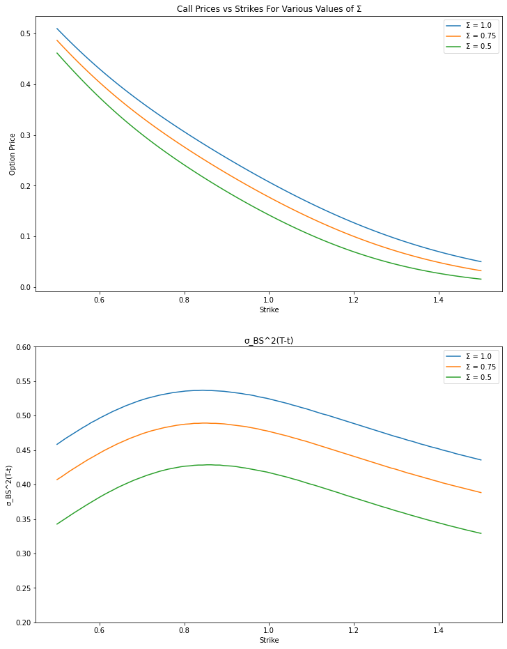
(a)

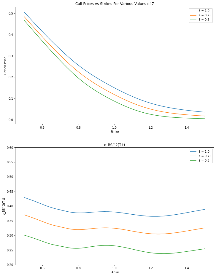
(b)

Figure 1. $\sigma^{2}_{BS}(T-t)$ of Call Options with Gaussian Mixture as log price distribution

3.2. Examples of volatility dynamics

Our goal in this subsection is to establish a general sufficient condition for existence of exponential moments in Assumption 2.1, (3), and to apply it to two specific examples of commonly used volatility models, namely the classical CIR model and its fractional counterpart. Without loss of generality, we assume that $T=1$ in throughout this subsection.

3.2.1. A general sufficient condition

Our sufficient condition, stated in Proposition 3.1 below, is based on the classical Garsia-Rodemich-Rumsey inquality (see Garsia et al., (1970)) whose statement we reproduce here for the convenience of the reader:

Theorem 3.1 (Garsia, Rodemich and Rumsey inequality).

Suppose that $\Psi$ and $p$ are continuous and strictly increasing, $\Psi(0)=p(0)=0$ and $\Psi(x)\to\infty$, as $x\to\infty$. For a continuous function $f:[0,1]\to{\mathbb{R}}$ let

$$c=\int_{0}^{1}\int_{0}^{1}\Psi\Big{(}\frac{\left\lvert f(t)-f(s)\right\rvert}{p(\left\lvert t-s\right\rvert)}\Big{)}\,ds\,dt.$$

If $c<\infty$ then

$$\left\lvert f(t)-f(s)\right\rvert\leq 8\int_{0}^{t-s}\Psi^{-1}\Big{(}\frac{4c}{u^{2}}\Big{)}\,dp(u)\text{ for all }\,0\leq s<t\leq 1.$$

Lemma 3.1.

Let $X$ be a continuous process on $[0,1]$. For $\gamma_{0}\in(0,1)$ and $M>0$ let

$$F_{M}=\int_{0}^{1}\int_{0}^{1}\exp\left(M\frac{\left\lvert X_{t}-X_{s}\right\rvert}{\left\lvert t-s\right\rvert^{\gamma_{0}}}\right)\,dt\,ds.$$ (3.3)

If  $\mathbb{E}\left[F_{M}\right]<\infty$, for all $M>0$ then the pathwise $\gamma$-Hölder seminorm

$$\left\lvert X\right\rvert_{\gamma}=\operatorname*{esssup}_{0\leq s<t\leq 1}\frac{\left\lvert X_{t}-X_{s}\right\rvert}{\left\lvert t-s\right\rvert^{\gamma}}$$

admits all exponential moments, for each $\gamma\in[0,\gamma_{0})$.

Proof.

It follows directly from Theorem 3.1 with $p(u)=u^{{\gamma_{0}}}$ and $\Psi_{M}=\exp\left(Mx\right)-1$ that, for each $M>0$, with $F_{M}$ is as in the statement, we have

$$\left\lvert X\right\rvert_{\gamma}\leq L_{M}(4F_{M})\text{ where }L_{M}(x)=\sup_{r\in(0,1]}8r^{-\gamma}\int_{0}^{r}\Psi^{-1}_{M}\Big{(}\frac{x}{u^{2}}\Big{)}\,dp(u).$$

For $x\geq 2$ and $r\in(0,1)$ we have

$$M\int_{0}^{r}\Psi^{-1}_{M}\left(\frac{x}{u^{2}}\right)\,dp(u) ={{\gamma_{0}}}\int_{0}^{r}\log\left(1+\frac{x}{u^{2}}\right)u^{{{\gamma_{0}}}-1}\,du\leq{{\gamma_{0}}}\int_{0}^{r}\log\left(\frac{3}{2}\frac{x}{u^{2}}\right)u^{{{\gamma_{0}}}-1}\,du\leq L(r),$$

where

$$L(r)=2{{\gamma_{0}}}\int_{0}^{r}\log\left(\frac{x}{u^{2}}\right)u^{{{\gamma_{0}}}-1}\,du=\frac{2r^{{\gamma_{0}}}}{{{\gamma_{0}}}}\left(2+{{\gamma_{0}}}\log\left(\frac{x}{r^{2}}\right)\right).$$

We pick $\gamma\in[0,{\gamma_{0}})$ and observe that for $x$ large enough,

namely $x\geq x_{0}:=\exp\left(\tfrac{2\gamma}{{{\gamma_{0}}}({{\gamma_{0}}}-\gamma)}\right)$, the function

$$r\mapsto 8r^{-\gamma}L(r)=8r^{{{\gamma_{0}}}-\gamma}(2+{{\gamma_{0}}}\log(x/r^{2}))$$

is non-decreasing on $(0,1]$. Therefore,

$$L_{M}(x)\leq\frac{2}{M}\left(\frac{2}{{{\gamma_{0}}}}+\log(\max(x,x_{0},2))\right),$$

so that, for each $k>0$ and each $M>0$, we have

$$\mathbb{E}\left[e^{k\left\lvert X\right\rvert_{\gamma}}\right]\leq e^{4k/(M{\gamma_{0}})}\mathbb{E}\left[e^{2k/M\log(\max(4F_{M},x_{0},2))}\right]=e^{4k/(M{\gamma_{0}})}\mathbb{E}\left[(\max(4F_{M},x_{0},2))^{2k/M}\right].$$

Given $k>0$, it remains to take $M=2k$ and use the assumption that $\mathbb{E}\left[F_{M}\right]<\infty$. ∎

Proposition 3.1.

Suppose that there exists constants $\varepsilon>0$ and ${\gamma_{0}}>0$ such that

$$\sup_{s\neq t\in[0,1]}\mathbb{E}\left[\exp\left(\varepsilon\frac{\left\lvert\sigma_{t}^{2}-\sigma^{2}_{s}\right\rvert}{\left\lvert t-s\right\rvert^{\gamma_{0}}}\right)\right]<\infty.$$

Then the $\gamma$-Hölder semi-norm of $\sigma$ admits all exponential moments for any $\gamma\in[0,{\gamma_{0}}/2)$.

Proof.

Using the elementary fact that $\lvert b-a\rvert\leq\sqrt{\left\lvert b^{2}-a^{2}\right\rvert}$ for all $a,b\geq 0$, followed by Young’s inequality, we obtain that for all $s\neq t\in[0,1]$, $M\geq 0$ and $\varepsilon\in(0,1)$ we have

$$M\frac{\left\lvert\sigma_{t}-\sigma_{s}\right\rvert}{\left\lvert t-s\right\rvert^{{\gamma_{0}}/2}}\leq M\sqrt{\frac{\left\lvert\sigma^{2}_{t}-\sigma^{2}_{s}\right\rvert}{\left\lvert t-s\right\rvert^{{\gamma_{0}}}}}\leq\varepsilon\frac{\left\lvert\sigma^{2}_{t}-\sigma^{2}_{s}\right\rvert}{\left\lvert t-s\right\rvert^{\gamma_{0}}}+\frac{M^{2}}{4\varepsilon}$$

We use Lemma 3.2 to conclude that

$$\mathbb{E}\left[\exp\left(M\frac{\left\lvert\sigma_{t}-\sigma_{s}\right\rvert}{\left\lvert t-s\right\rvert^{{\gamma_{0}}/2}}\right)\right]\leq{C\exp\left(C\varepsilon\kappa+\frac{M^{2}}{\varepsilon}\right)}<\infty,$$ (3.4)

Since the right-hand side of (3.4) is independent of $s,t$, we conclude that, for each $M$,

$$\sup_{s\neq t\in[0,1]}\mathbb{E}\left[\exp\left(M\frac{\left\lvert\sigma_{t}-\sigma_{s}\right\rvert}{\left\lvert t-s\right\rvert^{{\gamma_{0}}/2}}\right)\right]<\infty.$$

It remains to apply Lemma 3.1. ∎

3.2.2. CIR-based volatility

Let $(V_{t})$ be a nonnegative CIR process on $[0,1]$ started at $x>0$ at $t=0$. More precisely, we assume that $V$ admits the dynamics of the form

$$V_{t}=x+\int_{0}^{t}(a-kV_{s})\,ds+\int_{0}^{t}\eta\sqrt{V_{t}}\,dW_{t},$$ (3.5)

where $a,k,\eta>0$ are such that the Feller condition $2a\geq\eta^{2}$ is satisfied; consequently, $V_{t}\geq 0$ for all $t\in[0,1]$, a.s. An explicit formula for the moment-generating function of $V_{t}$ (see Alfonsi, (2015), Proposition 1.2.4, p. 7) is given by

$$\mathbb{E}\left[\exp\left(uV_{t}\right)\right]=F(t,u)^{2a/\eta^{2}}e^{u\exp\left(-kt\right)F(t,u)x},\text{ where }F(t,u)=\left(1-\frac{\eta^{2}}{2k}\left(1-e^{-kt}\right)u\right)^{-1},$$ (3.6)

for $u<u_{0}=2k\eta^{-2}(1-\exp\left(-k\right))^{-1}$.

Since $(1-e^{-1})\leq\tfrac{1}{s}(1-\exp\left(-s\right))\leq 1$, for all $s\in(0,1]$, there exist constants $0<c_{1}<c_{2}$, that depend only on $a,k$ and $\eta$, such that

$$(1-c_{1}\varepsilon\sqrt{t})^{-1}\leq F\left(t,\frac{\varepsilon}{\sqrt{t}}\right)\leq\left(1-c_{2}\varepsilon\sqrt{t}\right)^{-1}\text{ for }t\in(0,1]\text{ and }\varepsilon\in\left(-\infty,\tfrac{1}{2}\max(c_{1},c_{2})^{-1}\right).$$

Therefore, there exists a constant $C$ such that $\left\lvert F(t,\varepsilon/\sqrt{t})-1\right\rvert\leq C\sqrt{t}$ for $t\in(0,1]$ and $\varepsilon<\tfrac{1}{2}\max(c_{1},c_{2})^{-1}$. Perhaps with a different constant $C$ we then also have

$$\left\lvert\exp\left(-kt\right)F(t,\varepsilon/\sqrt{t})-1\right\rvert\leq C\sqrt{t}\text{ for }\varepsilon<\tfrac{1}{2}\max(c_{1},c_{2})^{-1}.$$ (3.7)

This estimate implies, in particular, that $F(t,\varepsilon/\sqrt{t})$ admits an upper bound, uniform in $t$ and all sufficiently small $\varepsilon$. Therefore, for $\varepsilon>0$ small enough, (3.6) and (3.7) imply that

$$\mathbb{E}\left[\exp\left(\varepsilon\frac{\left\lvert V_{t}-x\right\rvert}{\sqrt{t}}\right)\right] \leq\mathbb{E}\left[\exp\left(\varepsilon\frac{V_{t}-x}{\sqrt{t}}\right)\right]+\mathbb{E}\left[\exp\left(-\varepsilon\frac{V_{t}-x}{\sqrt{t}}\right)\right]$$

$$=F^{2a/\eta^{2}}\left(t,\frac{\varepsilon}{\sqrt{t}}\right)\Bigg{(}\exp\left(\frac{\varepsilon}{\sqrt{t}}x\left(\exp\left(-kt\right)F\left(t,\frac{\varepsilon}{\sqrt{t}}\right)-1\right)\right)$$

$$+\exp\left(\frac{\varepsilon}{\sqrt{t}}x\left(1-\exp\left(-kt\right)F\left(t,-\frac{\varepsilon}{\sqrt{t}}\right)\right)\right)\Bigg{)}\leq C\exp\left(C\varepsilon x\right),$$

for some constant $C$ which depends only on $a,k$ and $\eta$. Since $V$ is a homogeneous Markov process, we deduce that for all $0\leq s<t\leq 1$ and all $x\geq 0$, we have

$$\mathbb{E}\left[\exp\left(\varepsilon\frac{\left\lvert V_{t}-V_{s}\right\rvert}{\sqrt{t-s}}\right)\right]\leq C\mathbb{E}\left[\exp\left(C\varepsilon V_{t-s}\right)\right]$$

It follows directly from (3.6) that, for small enough $\varepsilon$, we have $\sup_{\delta\in[0,1]}\mathbb{E}\left[\exp\left(C\varepsilon V_{\delta}\right)\right]<\infty$. Therefore, the conditions of Proposition 3.1 are met, and, so for $0<\underline{\sigma}<\overline{\sigma}$, the process $\sigma_{t}=\underline{\sigma}+\min(\sqrt{V_{t}},\overline{\sigma})$ satisfies Assumption 2.1, (3).

3.2.3. The rough CIR model

Next, we consider a class of models driven by Volterra stochastic differential equations, including a truncation of the volatility process in the rough Heston model, as described in El Euch and Rosenbaum, (2019); Abi Jaber et al., (2019). We mention also that in Biagini et al., (2012) a Kyle’s model where the noise trading is assumed to be a fractional process is studied.

We fix $H\in(0,1/2)$, set $\alpha=H+1/2$ and let

$$K(t)=t^{\alpha-1}/\Gamma(\alpha)$$ (3.8)

be the $\alpha$-fractional kernel, where $\Gamma$ denotes the Gamma function. We choose two bounded continuous functions $b,s:{\mathbb{R}}\to{\mathbb{R}}$ and a constant $\kappa$ such that

$$\left\lvert b(x)\right\rvert,s^{2}(x)\leq\kappa,\text{ for all }x\in{\mathbb{R}}.$$

We also assume that the stochastic Volterra equation

$$V_{t}=V_{0}+\int_{0}^{t}K(t-u)b(V_{u})\,du+\int_{0}^{t}K(t-u)s(V_{u})\,dW_{u},\ t\in[0,1],$$ (3.9)

admits a strong solution. One sufficient condition is the Lipschitz continuity of the coefficients $b$ and $s$ (see Abi Jaber et al., (2019), Theorem 3.3., p. 3167). A (financially) more relevant case occurs when $b$ and $s$ define truncated Volterra square-root process, i.e., when

$$V_{t}=V_{0}+\int_{0}^{t}K(t-u)(b^{0}-b^{1}V_{u})\,du+\int_{0}^{t}K(t-u)\sqrt{A^{1}\min(V_{t},\overline{V})}\,dW_{u}$$ (3.10)

where $b^{0},b^{1},A^{1}$ and $\overline{V}$ are nonnegative constants. The existence, uniqueness and positivity theory of (3.10), parallels closely that of its version presented in Lemma 6.3, p. 3182 of Abi Jaber et al., (2019), so we do not go into details here.

Fix $0<\underline{\sigma}<\overline{\sigma}$. To show that the process $\sigma_{t}=\underline{\sigma}+\min(\sqrt{V_{t}},\overline{\sigma})$ satisfies Assumption 2.1, (3), we employ Proposition 3.1 above to $t\mapsto\sqrt{V_{t}}$. Lemma 3.2 below makes sure that its conditions are satisified.

Lemma 3.2.

There exists a constant $C>0$, which depends only on $\alpha$ and $\kappa$ such that

$$\mathbb{E}\left[\exp\left(\varepsilon\frac{\left\lvert V_{t}-V_{s}\right\rvert}{\left\lvert t-s\right\rvert^{H}}\right)\right]\leq{C\exp\left(C\varepsilon\kappa\right)}\text{ for all }s\neq t\text{ and }\varepsilon\in[0,1).$$ (3.11)

Proof.

Given $0\leq s<t\leq 1$, we decompose

$$V_{t}-V_{s}=A+M+D+N$$

where

$$A =\int_{0}^{s}(K(t-u)-K(s-u))b(V_{u})\,du$$

$$M =\int_{0}^{s}(K(t-u)-K(s-u))s(V_{u})\,dW_{u}$$

$$D =\int_{s}^{t}K(t-u)b(V_{u})\,du$$

$$N =\int_{s}^{t}K(t-u)s(V_{u})\,dW_{u}.$$

For $r\geq 0$, the Cauchy-Schwarz inequality implies that

$$\mathbb{E}\left[\exp\left(r\left\lvert V_{t}-V_{s}\right\rvert\right)\right] \leq\mathbb{E}\left[\exp\left(r(\left\lvert A\right\rvert+\left\lvert D\right\rvert)\right)\exp\left(r\left\lvert M+N\right\rvert\right)\right]$$

$$\leq\mathbb{E}\left[\exp\left(2r(\left\lvert A\right\rvert+\left\lvert D\right\rvert\right)\right]^{1/2}\mathbb{E}\left[\exp\left(2r\left\lvert M+N\right\rvert\right)\right]^{1/2}.$$

With $C$ denoting a generic constant, which may change from use to use and is allowed to depend only on $\alpha$ and $\kappa$, we have

$$\int_{s}^{t}K(t-u)\,du =C(t-s)^{\alpha}\text{ and }0\leq\int_{0}^{s}K(s-u)-K(t-u)\,du{=C(s^{\alpha}-t^{\alpha}+(t-s)^{\alpha})\leq}C(t-s)^{\alpha}.$$

Combining the equalities above with fact that $(t-s)^{\alpha}\leq(t-s)^{H}$, we obtain that

$$\left\lvert A\right\rvert \leq C\kappa\int_{0}^{s}(K(s-u)-K(t-u))\,du\leq C\kappa(t-s)^{\alpha}\leq C\kappa(t-s)^{H}\text{ and }$$

$$\left\lvert D\right\rvert \leq C\kappa\int_{s}^{t}K(t-u)\,du\leq C\kappa(t-s)^{\alpha}\leq C\kappa(t-s)^{H}$$

Consequently,

$$\mathbb{E}\left[\exp\left(2r(\left\lvert A\right\rvert+\left\lvert D\right\rvert)\right)\right]\leq{\exp\left(Cr\kappa(t-s)^{H}\right)}.$$ (3.12)

Turning to the $M+N$-term, we note that $M+N=\int_{0}^{t}H_{u}\,dW_{u}$ where

$$H_{u} =\begin{cases}(K(t-u)-K(s-u))s(V_{u})&u\in[0,s],\\ K(t-u)s(V_{u})&u\in[s,t].\end{cases}$$

Using the inequality $\mathbb{E}\left[\exp\left(\pm L_{t}\right)\right]\leq\mathbb{E}\left[\exp\left(2\left\langle L\right\rangle_{t}\right)\right]^{1/2}$, valid for any continuous local martingale $L$, we conclude that

$$\mathbb{E}\left[\exp\left(2r\left\lvert M+N\right\rvert\right)\right]\leq\mathbb{E}\left[\exp\left(2r(M+N)\right)\right]+\mathbb{E}\left[\exp\left(-2r(M+N)\right)\right]\leq 2\mathbb{E}\left[\exp\left(8r^{2}\int_{0}^{t}H_{u}^{2}\,du\right)\right]^{{1/2}}.$$

For $0\leq u\leq s\leq t$, we have that

$$0 \leq((s-u)^{\alpha-1}-(t-u)^{\alpha-1})^{2}\leq(s-u)^{2\alpha-2}-2(s-u)^{\alpha-1}(t-u)^{\alpha-1}+(t-u)^{2\alpha-2}$$

$$\leq(s-u)^{2\alpha-2}-(t-u)^{2\alpha-2}.$$

The (in)equalities

$$\int_{s}^{t}K(t-u)^{2}\,du =C(t-s)^{2\alpha-1}\text{ and }\int_{0}^{s}(K(t-u)-K(s-u))^{2}\,du\leq C(t-s)^{2\alpha-1}$$

further yield

$$\mathbb{E}\left[\exp\left(2r\left\lvert M+N\right\rvert\right)\right] \leq 2\mathbb{E}\left[\exp\left(8r^{2}\Big{(}\int_{0}^{s}(K(s-u)-K(t-u))^{2}\eta(V_{u})^{2}\,du+\int_{s}^{t}K(t-u)^{2}(\eta(V_{u}))^{2}\,du\Big{)}\right)\right]^{{1/2}}$$

$$\leq 2{\exp\left(Cr^{2}\kappa(t-s)^{2\alpha-1}\right)}^{{1/2}}.$$

Since $(t-s)^{2\alpha-1}=(t-s)^{2H}$, this implies that

$$\mathbb{E}\left[\exp\left(2r|M+N|\right)\right]\leq 2{\exp\left(C\Big{(}r(t-s)^{H}\Big{)}^{2}\kappa\right)}^{{1/2}}$$ (3.13)

If we replace $r$ by $\varepsilon/(t-s)^{H}$, combine the estimates (3.12) and (3.13) above, and use that $\varepsilon^{2}<\varepsilon$ for $\varepsilon\in[0,1)$, we get

$$\mathbb{E}\left[\exp\left(\varepsilon\tfrac{|V_{t}-V_{s}|}{\left\lvert t-s\right\rvert^{H}}\right)\right] \leq\sqrt{2}{\exp\left(C\varepsilon\kappa\right)}^{1/2}{\exp\left(C\varepsilon^{2}\kappa\right)}^{1/4}\leq C{\exp\left(C\varepsilon\kappa\right)}\qed$$

4. Proofs

We divide this section into two parts. In the first part we work towards the proof of the Proposition 2.1, while he second one focuses on the proof of the main Theorem 2.1. We refer the reader to subsection 2.4 above for all unexplained notation.

4.1. Proof of Proposition 2.1

We start with a modest generalization of the standard existence and comparison result for Lipschitz BSDE in a special case.

Lemma 4.1.

1. (Existence) Suppose that the random field $f:[0,T]\times\Omega\times{\mathbb{R}}\to{\mathbb{R}}$ is $\mathcal{F}^{W}$-progressively measurable, $f(t,0)\in\mathcal{S}^{\infty}$,

   $$|f(t,y^{\prime})-f(t,y)|\leq C|y^{\prime}-y|\text{ for all $y,y^{\prime}\in{\mathbb{R}}$ and all $t$, a.s.}$$ (4.1)

   and that $b$ is a $\operatorname{bmo}$ process. Then the BSDE

   $$y_{t}=\int_{t}^{T}\Big{(}f(u,y_{u})+z_{u}b_{u}\Big{)}\,du+\int_{t}^{T}z_{u}\,dW_{u},$$ (4.2)

   admits a solution $(y,z)\in\mathcal{S}^{\infty}\times\operatorname{bmo}$.

2. (Comparison) Suppose that $b\in\operatorname{bmo}$, $f^{1}$ and $f^{2}$ are $\mathcal{F}^{W}$-progressive random fields which satisfy (4.1) above and $f^{1}(t,y)\leq f^{2}(t,y)$ for all $t,y$, a.s. If $(y^{1},z^{1})$ and $(y^{2},z^{2})$ in $\mathcal{S}^{\infty}\times\operatorname{bmo}$ satisfy

   $$y^{i}=\int_{t}^{T}(f^{i}(u,y^{i}_{u})+z^{i}_{u}\,b_{u})\,du+\int_{t}^{T}z^{i}_{u}\,dW_{u},$$

   then $y^{1}_{t}\geq y^{2}_{t}$, for all $t$, a.s. In particular, the solution in 1. above is unique.

Proof.

(1)  Let $\Gamma_{t}=\mathcal{E}(\int_{0}^{t}b_{u}\,dW_{u})$, and let $\mathbb{E}^{b}$ denote the expectation under the probability measure $\mathbb{P}^{b}$ defined by $d\mathbb{P}^{b}=\Gamma_{T}\,d\mathbb{P}$. We define $\Phi:\mathcal{S}^{\infty}\to\mathcal{S}^{\infty}$ by

$$\Phi(y)_{t}=\mathbb{E}^{#1}\left[\int_{t}^{T}f(u,y_{u})\,du\nonscript\>\middle|\nonscript\>\mathopen{}\mathcal{F}^{W}_{t}\right]$$

and note that the Lipschitz property of $f$ implies that

$$\|{\Phi(y^{2})_{t}-\Phi(y^{1})_{t}}\|_{L^{\infty}}\leq C\int_{t}^{T}\|{y^{2}_{u}-y^{1}_{u}}\|_{L^{\infty}}\,du.$$

From there, it follows immediately that $\Phi$ is a contraction on $\mathcal{S}^{\infty}$ equipped with the (Banach) norm $\|y\|_{w}=\sup_{t}e^{2Ct}\|y_{t}\|_{L^{\infty}}$. The fixed point $\hat{y}$ of $\Phi$ has the property that $\hat{y}_{T}=0$ and $\Gamma_{t}\hat{y}_{t}+\int_{0}^{t}\Gamma_{u}f(u,\hat{y}_{u})\,du$ is a $\mathbb{P}^{b}$-martingale satisfying

$$\sup_{t\in[0,T]}|\Gamma_{t}\hat{y}_{t}|+\int_{0}^{t}|\Gamma_{u}f(u,\hat{y}_{u})|\,du\leq C\sup_{0\leq t\leq T}|\Gamma_{t}|.$$

Theorem 3.1., p. 57, in Kazamaki, (2006) applied to $\Gamma$ and the martingale representation theorem imply that (4.2) holds for some progressive process $\hat{z}$ with $\mathbb{E}^{b}\left[\sqrt{\int_{0}^{T}\hat{z}_{u}^{2}}\,du\right]<\infty$. Since $\hat{y}_{t}$ and $f(t,\hat{y}_{t})$ are both bounded processes, the process $\int_{0}^{t}\hat{z}_{u}(-b_{u}\,du+dW_{u})$ is a bounded $\mathbb{P}^{b}$-local martingale, and, therefore, a $\mathbb{P}^{b}$-BMO martingale. Thanks to the invariance of $\operatorname{bmo}$ spaces under equivalent measure changes (see (Kazamaki,, 2006, Theorem 3.3., p. 57)), $\hat{z}$ is a bmo process with respect to $\mathbb{P}$, as well.

(2) This can be proved using the standard linearization method (see, e.g., the proof of (Zhang,, 2017, Theorem 4.4.1, p. 87)) while keeping in mind the fact that $\mathcal{E}(\int_{0}^{\cdot}b_{u}\,dW_{u})$ is a uniformly integrable martingale as soon as $b$ is a $\operatorname{bmo}$-process (see (Kazamaki,, 2006, Theorem 2.3, p. 31)). ∎

Proof of Proposition 2.1.

The first step is to solve the auxiliary BSDE

$$y_{t}=\int_{t}^{T}\Big{(}\frac{\tilde{J}^{2}_{u}}{2y_{u}}-z_{u}\psi_{u}\Big{)}\,du+\int_{t}^{T}z_{u}\,dW_{u},$$ (4.3)

where $\tilde{J}_{t}=\hat{\rho}J_{t}$ and $\psi$ is given by $L=L_{0}\mathcal{E}(\int_{0}^{\cdot}\psi_{t}\,dW_{t})$. To do that, we pose a sequence of BSDEs

$$y^{n}_{t}=\int_{t}^{T}\Big{(}\frac{\tilde{J}^{2}_{u}}{2(\tfrac{1}{n}\tilde{J}_{0}+|y^{n}_{u}|)}-z^{n}_{u}\psi_{u}\Big{)}\,du+\int_{t}^{T}z^{n}_{u}\,dW_{u},$$ (4.4)

each of which has a unique solution $(y^{n},z^{n})\in\mathcal{S}^{\infty}\times\operatorname{bmo}$ by Lemma 4.1, (1) above. The second part of the same Lemma implies that

$$n_{1}\leq n_{2}\rightarrow y^{n_{1}}_{t}\leq y^{n_{2}}_{t}\text{ for all }t\in[0,T],\text{ a.s.}.$$

Assuming, without loss of generality, that we are working on the canonical space $C[0,T]$, we define the adapted processes

$$\tilde{J}^{+}(t,\omega)=\sup_{s\geq t,\tilde{\omega}}{|\tilde{J}_{s}(\omega\oplus_{t}\tilde{\omega})|},\,\tilde{J}^{-}(t,\omega)=\inf_{s\geq t,\tilde{\omega}}{|\tilde{J}_{s}(\omega\oplus_{t}\tilde{\omega})|}$$

and for fixed $t\in[0,T]$ consider two additional families of BSDEs

$$y^{t,\pm,n}_{s}=\int_{s}^{T}\Big{(}\frac{(\tilde{J}_{t}^{\pm})^{2}}{2(\tfrac{1}{n}\tilde{J}_{0}+|y^{t,\pm,n}_{u}|)}-z^{t,\pm,n}_{u}\psi_{u}\Big{)}\,du+\int_{s}^{T}z^{t,\pm,n}_{u}\,dW_{u}.$$ (4.5)

For each $n\in{\mathbb{N}}$, these equations admit positive deterministic (conditionally on $\mathcal{F}^{W}_{t}$) solutions:

$$y^{t,\pm,n}_{s} =\sqrt{\tfrac{\tilde{J}_{0}^{2}}{n^{2}}+(\tilde{J}^{\pm}_{t})^{2}(T-s)}-\frac{\tilde{J}_{0}}{n},\ z^{t,\pm,n}_{s}=0.$$

Moreover, since Lemma 4.1, (2) applies to these equations as well, we have

$$y^{n}_{t}\leq y^{t,+,n}_{t}\leq\tilde{J}^{+}_{t}\sqrt{T-t}$$

as well as

$$\tfrac{1}{n}\tilde{J}_{0}+y^{n}_{t}\geq\tfrac{1}{n}\tilde{J}_{0}+y^{t,-,n}_{t}\geq\tilde{J}^{-}_{t}\sqrt{T-t}..$$ (4.6)

Combining both inequalities, we obtain the following estimates:

$$\tilde{J}^{-}_{t}\sqrt{T-t}-\tfrac{1}{n}\tilde{J}_{0}\leq y^{n}_{t}\leq\tilde{J}^{+}_{t}\sqrt{T-t}$$ (4.7)

Let the process $y$ be defined by $y_{t}=\liminf_{n\to\infty}y^{n}_{t}$. It is progressively measurable and we have $y_{t}=\lim_{n}y^{n}_{t}$, a.s., for each $t$. Thanks to (4.7) the sequence $(\tilde{J}_{0}/n+y^{n}_{t})^{-1}$ is dominated by the integrable function $(T-t)^{-1/2}$ (up to a multiplicative constant), so that the dominated convergence theorem can be applied to pass to the limit $n\to\infty$ on both sides of the equality $y^{n}_{t}=\mathbb{E}^{\psi}_{t}[\int_{t}^{T}\tilde{J}^{2}_{u}/(2\tilde{J}_{0}/n+2y^{n}_{u})\,du]$ to conclude that

$$y_{t}=\mathbb{E}^{\psi}_{t}\left[\int_{t}^{T}\frac{\tilde{J}^{2}_{u}}{2y_{u}}\,du\right],\text{ a.s., for each $t$.}$$

The fact the augmented filtration of $W^{\psi}=W-\int_{0}^{\cdot}\psi_{u}\,du$ is Brownian allows us to show that $y$ admits a continuous modification, and, then, as in the proof of Lemma 4.1 above, that $(y,z)$ satisfy the BSDE (4.3) for some $z\in\operatorname{bmo}$.

Passing to the limit in (4.7) we obtain

$$\tilde{J}^{-}_{t}\leq h_{t}\leq\tilde{J}^{+}_{t}\text{ where }h_{t}=\frac{y_{t}}{\sqrt{T-t}}.$$ (4.8)

The two bounds above imply that $h$ is positive, bounded, bounded away from $0$ and $\lim_{t\to T}h_{t}=\tilde{J}_{T}$. Recalling that $|\tilde{J}|_{\gamma}$ denotes the $\gamma$-Holder norm of $\tilde{J}$, Itô’s formula yields the following dynamics for $h$ on $[0,T)$

$$dh_{t}=\Big{(}a_{t}+K_{t}\,\psi_{t}\Big{)}\,dt-K_{t}\,dW_{t},$$

where $a_{t}=\tfrac{\tilde{J}_{t}+h_{t}}{2h_{t}}\frac{h_{t}-\tilde{J}_{t}}{T-t}$ is bounded by $\left(\frac{\tilde{J}_{t}}{2h_{t}}+\frac{1}{2}\right)|\tilde{J}|_{\gamma}|T-t|^{1-\gamma}$ and $K_{t}=\tfrac{z_{t}}{\sqrt{T-t}}=\frac{h_{t}z_{t}}{y_{t}}$. We apply Itô’s formula a second time to obtain

$$d\ln h_{t}=\left(\frac{a_{t}}{h_{t}}+\frac{1}{2}\psi^{2}_{t}-\frac{1}{2}\left(\frac{z_{t}}{y_{t}}-\psi_{t}\right)^{2}\right)\,dt-\frac{z_{t}}{y_{t}}\,dW_{t}$$

which thanks to the identity $\sigma_{t}=L_{t}J_{t}=J_{t}e^{\int_{0}^{t}\psi_{s}dW_{s}-\frac{1}{2}\int_{0}^{t}\psi_{s}^{2}ds}$ leads to identity

$$\frac{h_{t}}{J_{t}e^{\int_{0}^{t}\frac{a_{s}}{h_{s}}\,ds}}\sigma_{t}=h_{0}e^{\int_{0}^{t}\psi_{s}-\frac{z_{s}}{y_{s}}\,dW_{s}-\frac{1}{2}\int_{0}^{t}\left(\psi_{s}-\frac{z_{s}}{y_{s}}\right)^{2}ds}.$$ (4.9)

Assumption 2.1, (3) and the bounds of $a$ imply that the term $e^{\int_{0}^{t}\frac{a_{s}}{h_{s}}\,ds}$ admits all moments. The right hand side of (4.9) is proportional to $1/\lambda_{t}$. In fact a direct computation shows that (4.9) leads to

$$\hat{\rho}^{2}\sigma_{t}=\sqrt{T}h_{0}\sigma_{0}\gamma_{t}e^{\int_{0}^{t}\psi_{s}-\frac{z_{s}}{y_{s}}\,dW_{s}-\frac{1}{2}\int_{0}^{t}\left(\psi_{s}-\frac{z_{s}}{y_{s}}\right)^{2}ds}.$$ (4.10)

where $\gamma_{t}:=\tilde{J}_{t}\frac{e^{\int_{0}^{t}\frac{a_{s}}{h_{s}}\,ds}}{h_{t}\sqrt{T}}$. We can compute

$$\int_{0}^{T}\gamma^{2}_{t}dt =\int_{0}^{T}\frac{\tilde{J}^{2}_{t}}{Th^{2}_{t}}e^{\int_{0}^{t}2\frac{a_{s}}{h_{s}}\,ds}dt=\int_{0}^{T}\frac{\tilde{J}^{2}_{t}}{Th^{2}_{t}}e^{\int_{0}^{t}\frac{1-\tilde{J}^{2}_{s}/h^{2}_{s}}{(T-s)}\,ds}dt$$

$$=\int_{0}^{T}\frac{\tilde{J}^{2}_{t}}{h^{2}_{t}(T-t)}e^{-\int_{0}^{t}\frac{\tilde{J}^{2}_{s}}{(T-s)h^{2}_{s}}\,ds}dt=1$$

which is deterministic.

As the last step in the existence proof, we define $G_{t}=y_{t}^{2}L_{t}^{2}$ where $L_{t}=\mathcal{E}(\int_{0}^{\cdot}\psi_{u}\,dW_{u})$. A direct computation implies that $G$ satisfies the original BSDE (2.8) with

$${U_{t}}={2G_{t}}\Big{(}\psi_{t}-\frac{z_{t}}{y_{t}}\Big{)}.$$ (4.11)

Since $\psi\in\operatorname{bmo}$, $y_{t}\geq C\sqrt{T-t}$ for some constant $C$ and $z_{t}/\sqrt{T-t}\in\operatorname{bmo}$, the equality (4.11) above implies that $\tfrac{U}{G}\in\operatorname{bmo}$. On the other hand, the relation (4.8) implies that $G_{t}\leq\eta(T-t)$ for some strictly positive random variable $\eta$. With $\sigma$ being continuous and bounded away from $0$, this implies that $\int_{0}^{T}\tfrac{\sigma_{s}^{2}}{G_{s}}\,ds=\infty$, a.s.

To prove uniqueness, let $(G^{i},U^{i})\in\mathcal{S}^{+}_{0}\times\mathcal{P}^{2}$ for $i=1,2$ be two solutions of (2.8). By a direct computation, $y^{i}=\frac{\sqrt{G^{i}}}{L}$ solves (4.3). We define $\delta y=y^{2}-y^{1}$ and $\delta z=z^{2}-z^{1}$, and observe that

$$d\delta y_{t}=r_{t}\delta y_{t}\,dt+\delta z_{t}(dW_{t}+\psi\,dt)\text{ where }r_{t}=\frac{\tilde{J}^{2}_{t}}{2y^{1}_{t}y^{2}_{t}}$$

on $[0,T)$. Since $r_{t}\geq 0$, the process $R$ defined by $R_{t}=\exp\left(-\int_{0}^{t}r_{u}\,du\right)$ for $t<T$ is positive and bounded, and admits a limit as $t\to T$. Itô’s formula implies that $R_{t}\delta y_{t}$ is a bounded local martingale on $[0,T)$ with $R_{t}\delta y_{t}\to 0$ as $t\to T$. It follows that $R_{t}\delta y_{t}$ is a uniformly integrable martingale with the last element $0$ so that $R_{t}\delta y_{t}=0$, for all $t$. since $R_{t}>0$ for $t<T$, we conclude that $y^{1}_{t}=y^{2}_{t}$ for all $t$, a.s., and $z^{1}=z^{2}$ $\text{Leb}\times\mathbb{P}$-a.e. ∎

4.2. Proof of Theorem 2.1

The proof starts with the introduction of several processes used in the construction of the novel state process $\xi^{*}$ of (2.14). After that, Lemma 4.2 collects some of their essential properties and establishes the existence and uniqueness of $\xi^{*}$; it also features three other facts needed in the sequel. The rest of this subsection lays out the details of the proof and is divided into several subsections. We refer the reader to subsection 2.4 above for all unexplained notation, and note that Assumption 2.1 is in force throughout.

We start with the auxiliary $\mathcal{F}^{W,B}$-martingale $\hat{Z}$ given by

$$\hat{Z}_{t}=\int_{0}^{t}\hat{\rho}\lambda_{s}\sigma_{s}\,dB_{s},$$ (4.12)

which, by the Dambis-Dubins-Schwarz theorem, admits the representation

$$\hat{Z}_{t}=\beta_{\langle\hat{Z}\rangle_{t}}\text{ where }\langle\hat{Z}\rangle_{t}=\int_{0}^{t}\hat{\rho}^{2}\lambda_{s}^{2}\sigma_{s}^{2}\,ds=1-\Sigma_{t}\in\mathcal{F}^{W}_{t},$$

and where $\beta$ is an $\mathcal{F}^{W,B}$-Brownian motion given by

$$\beta_{u}=\hat{Z}_{\Gamma_{u}}\text{ where }\Gamma_{u}=\inf\{t\geq 0\,:\,1-\Sigma_{t}=u\},$$ (4.13)

which satisfy $\Gamma_{1-\Sigma_{t}}=t$ amd $1-\Sigma_{\Gamma_{u}}=u$ thanks to continuity and strict monotonicity of $\Sigma_{T}$. With $\hat{\xi}$ defined on $[0,1]$ by

$$\hat{\xi}_{t}=th^{-1}(\tilde{v})+(1-t)\int_{0}^{t}\frac{1}{1-s}\,d\beta_{s},\text{ for }t\in[0,1)\text{ and }\hat{\xi}_{1}=h^{-1}(\tilde{v}),$$ (4.14)

we set

$$\xi^{*}_{t}=\hat{\xi}_{1-\Sigma_{t}}.$$

Lemma 4.2.

1. For all $\xi\in{\mathbb{R}}$ and $u\in(0,1]$, we have

   $$\int\left(\int_{0}^{\xi+\zeta}\left\lvert h(x)\right\rvert\,dx\right)p(u,\zeta)\,d\zeta<\infty.$$

2. The Brownian motion $\beta$ is independent of $W$ and $\tilde{v}$.

3. Conditionally on $\tilde{v}$, $\hat{\xi}$ is a Brownian bridge from $0$ to $h^{-1}(\tilde{v})$ and admits the following dynamics:

   $$d\hat{\xi}_{t}=\frac{h^{-1}(\tilde{v})-\hat{\xi}_{t}}{1-t}\,dt+d\beta_{t}\text{ for }t\in[0,1),\ \lim_{t\to 1}\hat{\xi}_{t}=\hat{\xi}_{1}=h^{-1}(\tilde{v}),\text{ a.s.}$$ (4.15)

4. $\hat{\xi}$ is a Brownian motion independent of $W$.

5. For $u\in[0,1]$ and $p\in[1,2]$ we have

   $$\mathbb{E}\left[\left\lvert R_{\xi}(1-u,\hat{\xi}_{u})\right\rvert^{p}\right]\leq\mathbb{E}\left[\left\lvert\tilde{v}\right\rvert^{p}\right]<\infty.$$ (4.16)

6. $\mathbb{E}\left[R^{c}(0,\tilde{v})\right]<\infty$.

7. The random variable $\xi^{*}_{T}$ is $\mathcal{F}^{\xi^{*},W}_{t}$-conditionally normal with mean $\xi^{*}_{t}$ and variance $\Sigma_{t}$. In particular, $\xi^{*}$ is an $\mathcal{F}^{\xi^{*},W}$-martingale.

8. The process $\xi^{*}$ is a continuous $\mathcal{F}$-semimartingale on $[0,T]$, orthogonal to $W$. Moreover, it is the unique continuous process that satisfies (2.14) on $[0,T)$.

9. We have

   $$d\xi^{*}_{t}=\lambda_{t}\,d\hat{Y}^{*}_{t},$$ (4.17)

   and the pairs $(\xi^{*},W)$, $(\hat{Y}^{*},W)$ and $(Y,W)$ all generate the same filtration.

Proof.

1. Using the monotonicity of $h$ to justify the inequality $\left\lvert h(\xi+\sqrt{u}y)\right\rvert\leq\left\lvert h(\xi)\right\rvert+\left\lvert h(y+\xi)\right\rvert$, for $u\in[0,1]$, and a simple change of variables, we obtain

   $$\int \left(\int_{0}^{\xi+\zeta}\left\lvert h(x)\right\rvert\,dx\right)p(u,\zeta)\,d\zeta=\int\left(\int_{0}^{\xi+y\sqrt{u}}\left\lvert h(x)\right\rvert\,dx\right)p(1,y)\,dy\leq$$

   $$\leq\int\max\Big{(}\left\lvert h(\xi+\sqrt{u}y)\right\rvert,\left\lvert h(0)\right\rvert\Big{)}\left\lvert\xi+y\sqrt{u}\right\rvert p(1,y)\,dy$$

   $$\leq\int\Big{(}\left\lvert h(0)\right\rvert+\left\lvert h(\xi)\right\rvert+\left\lvert h(\xi+y)\right\rvert\Big{)}\left\lvert\xi+y\sqrt{u}\right\rvert p(1,y)\,dy$$

   $$\leq C+C\int\left\lvert h(r)\right\rvert(1+\left\lvert r\right\rvert)p(1,r-\xi)\,dr=C+C\int\left\lvert h(r)\right\rvert(1+\left\lvert r\right\rvert)e^{-\xi^{2}/2}e^{\xi r}p(1,r)\,dr$$

   where $C$ is a finite constant which depends on $h$ and $\xi$. The last integral is finite by the Cauchy-Schwarz inequality because both $h(r)$ and $(1+\left\lvert r\right\rvert)e^{\xi r}$ are square-integrable with respect to the Gaussian measure with density $p(1,r)$.

2. Since $\hat{Z}$ is a Brownian motion independent of $W$ and $\tilde{v}$, and $\Gamma$ is a time change with respect to $\mathcal{F}^{W}$, the process $\beta$ is a continuous martingale, conditionally on $W$. Its quadratic variation is Brownian, so, by Lévy’s criterion, $\beta$ is a Brownian motion independent of $W$ and $\tilde{v}$.

3. By its definition, $\beta$ is independent of $\tilde{v}$, so $\hat{\xi}$ is a Gaussian process conditionally on $\tilde{v}$. Moreover, its conditional mean and covariance functions, namely $th^{-1}(\tilde{v})$ and $\min(s,t)-st$, match those of the Brownian bridge from $0$ to $h^{-1}(\tilde{v})$. The dynamics (4.15) is a direct consequence of Itô’s formula.

4. The process $\hat{\xi}$ is $\mathcal{F}^{\beta,\tilde{v}}$-adapted and both $\beta$ and $\tilde{v}$ are independent of $W$, as established in (2) above, so $\hat{\xi}$ is independent of $\mathcal{F}^{W}$. To see that it is a Brownian motion, it is enough to observe that it is a Brownian bridge from $0$ to an independent standard normal (or simply compute its mean and covariance functions as above).

5. Since $R_{\xi}(1-\cdot,\cdot)$ is a space-time harmonic function and $\hat{\xi}$ is a Brownian motion, $V_{u}=R_{\xi}(1-u,\hat{\xi}_{u})$ is a martingale with the terminal condition $R_{\xi}(0,\hat{\xi}_{1})=\tilde{v}$ and the inequality (4.16) is a direct consequence of Jensen’s inequality.

6. Using the fact that the supremum in

   $$R^{c}(0,\tilde{v})=\sup_{\xi\in{\mathbb{R}}}\Big{(}\xi\tilde{v}-\int_{0}^{\xi}h(x)\,dx\Big{)}$$

   is attained at $\xi=h^{-1}(\tilde{v})$, we obtain

   $$R^{c}(0,\tilde{v}) =\left\lvert\tilde{v}h^{-1}(\tilde{v})-\int_{0}^{h^{-1}(\tilde{v})}h(x)\,dx\right\rvert=\left\lvert\int_{0}^{h^{-1}(\tilde{v})}(\tilde{v}-h(x))\,dx\right\rvert$$

   $$\leq\left\lvert h^{-1}(\tilde{v})\right\rvert\max_{r\in[0,1]}\Big{\lvert}\tilde{v}-h(rh^{-1}(\tilde{v}))\Big{\rvert}\leq\left\lvert h^{-1}(\tilde{v})\right\rvert\Big{(}\left\lvert\tilde{v}\right\rvert+\left\lvert h(0)\right\rvert\Big{)},$$

   where the last inequality follows from the monotonicity of $h$. The random variable $h^{-1}(\tilde{v})$ is normally distributed and therefore in $\mathbb{L}^{2}$, and so, by Assumption 2.1, (2), both $h(0)h^{-1}(\tilde{v})$ and $h^{-1}(\tilde{v})\tilde{v}$ belong to $\mathbb{L}^{1}$.

7. $\hat{\xi}$ is a Brownian motion independent of $W$ and $\Sigma$ is $\mathcal{F}^{W}$-adapted. Therefore, conditionally on $\mathcal{F}^{W}_{T}$, $\xi^{*}_{t}=\hat{\xi}_{1-\Sigma_{t}}$ is a centered Gaussian process with independent increments and deterministic variance function $1-\Sigma_{t}$. Therefore, conditionally on $\mathcal{F}^{W}_{T}\vee\mathcal{F}^{\xi^{*}}_{t}$, the random variable $\xi^{*}_{T}$ is normally distributed with mean $\xi^{*}_{t}$ and variance $\Sigma_{t}$. The statement now follows by further conditioning on $\mathcal{F}^{W}_{t}$.

8. To show that $\xi^{*}$ solves (2.14), we use (4.15) to get the following representation

   $$\xi^{*}_{t}=\int_{0}^{1-\Sigma_{t}}\frac{h^{-1}(\tilde{v})-\hat{\xi}_{u}}{1-u}\,du+\beta_{1-\Sigma_{t}}=\int_{0}^{t}\frac{h^{-1}(\tilde{v})-\xi^{*}_{s}}{\Sigma_{s}}\,\hat{\rho}^{2}\sigma^{2}_{s}\lambda^{2}_{s}\,ds,+\hat{Z}_{t},\ t\in[0,T)$$

   where we used the change of variable $s=\Sigma^{-1}_{1-u}$. Since $d\hat{Z}=\hat{\rho}\lambda\sigma\,dB$, $\xi^{*}$ indeed satisfies (2.14).

   For uniqueness, it suffices to note that the equation for the difference of two solutions a linear ODE with random coefficients. These coefficients are bounded a.s., on $[0,t]$ for each $t<T$, and our claim follows from Gronwall’s inequality.

   By (4.15) above, $\hat{\xi}$ is a Brownian bridge, conditionally on $\tilde{v}$. Therefore, we have

   $$\int_{0}^{1}\frac{\lvert h^{-1}(\tilde{v})-\hat{\xi}_{u}\rvert}{1-u}\,du<\infty,\text{ a.s.}$$

   The same change of variable as above, namely $s=\Sigma^{-1}_{1-u}$, allows us to conclude that (2.14) provides an $\mathcal{F}$-semimartingale decomposition of $\xi^{*}$ on the entire $[0,T]$. The orthogonality with $W$ is the direct consequence of the fact that $W$ and $B$ are orthogonal.

9. The identity (4.17) follows directly from (2.14). Since $\lambda$ is bounded and bounded away from $0$, $(\xi^{*},W)$ and $(\hat{Y}^{*},W)$ generate the same filtration. The pairs $(\hat{Y}^{*},W)$ and $(Y,W)$ generate the same filtratoin because the difference $Y^{*}-\hat{Y}^{*}$ is $\mathcal{F}^{W}$-adapted. ∎

4.2.1. An expression for $\Pi(X,\bm{P}^{*}(X+Z))$

Let $X$ be a trading strategy, $Y=X+Z$, $\hat{Y}=X-\int_{0}^{\cdot}\rho\sigma_{s}\,dW_{s}$, $\xi=\bm{\xi}^{*}(Y)$, and $P=\bm{P}^{*}(Y)$, with the functionals $\bm{\xi}^{*}$ and $\bm{P}^{*}$ defined in (2.12) and (2.13) above. We also introduce the following shortcuts for a generic function $F$:

$$(\Delta F)_{t}=F(\Sigma_{t},\xi_{t})-F(\Sigma_{t},\xi_{t-}),\text{ and }(\Delta^{2,\pm}F)_{t}=(\Delta F)_{t}-F_{\xi}(\Sigma_{t},\xi_{t\pm})\Delta\xi_{t}.$$

Thanks to Itô’s lemma, we have the following expressions for the dynamics of $P$ and $[P,X]$:

$$dP_{t} =-\hat{\rho}^{2}\lambda^{2}_{t}\sigma_{t}^{2}R_{\xi t}(\Sigma_{t},\xi_{t-})\,dt+R_{\xi\xi}(\Sigma_{t},\xi_{t-})\,d\xi_{t}+\frac{1}{2}R_{\xi\xi\xi}(\Sigma_{t},\xi_{t-})d[\xi,\xi]^{c}_{t}+(\Delta^{2,-}R_{\xi})_{t},$$

$$d[P,X]_{t} =\lambda_{t}R_{\xi\xi}(\Sigma_{t},\xi_{t-})\Big{(}d[X,X]^{c}+\hat{\rho}\sigma_{t}\,d[X,B]^{c}\Big{)}+(\Delta R_{\xi})_{t}\Delta X_{t}.$$

Since $(\Delta^{2-}R)_{t}+(\Delta R_{\xi})_{t}\Delta\xi_{t}=(\Delta^{2+}R)_{t}$, applying Ito’s formula to $\frac{\tilde{v}\xi_{t}-R(\Sigma_{t},\xi_{t})}{\lambda_{t}}$ and rearranging terms, it follows that

$$\Pi(X,P)_{t}=\int_{0}^{t}(\tilde{v}-P_{s-})dX_{s}-[P,X]_{t}=(I)+(II)+(III)+(IV),$$ (4.18)

where

$$\begin{split}(I)&=\frac{\tilde{v}\xi_{t}-R(\Sigma_{t},\xi_{t})}{\lambda_{t}}+\frac{R(1,0)}{\lambda_{0}},\\ (II)&=-\int_{0}^{t}\lambda_{s}\frac{R_{\xi\xi}(\Sigma_{s},\xi_{s-})}{2}\,d[X]^{c}+\sum_{s\leq t}(\Delta^{2,+}R)_{s},\\ (III)&=\int_{0}^{t}(R(\Sigma_{s},\xi_{s-})-\tilde{v}\xi_{s-})\,d\frac{1}{\lambda_{s}}\text{ and }\\ (IV)&=\hat{\rho}\int_{0}^{t}(P_{s-}-\tilde{v})\sigma_{s}dB_{s}.\end{split}$$ (4.19)

4.2.2. An upper bound for $\bm{P}^{*}$-admissible strategies

Suppose now that $X$ is $\bm{P}^{*}$-admissible and let $P=\bm{P}^{*}(X+Z)$. Moreover, let $(\tau_{n})$ be a common reducing sequence for the $(\mathcal{F}_{t})$-local martingales in $(III)$ and $(IV)$ of (4.19). By the convexity of $R(\Sigma_{t},\cdot)$, we have $\Delta^{2,+}R_{t}\leq 0\leq\Delta^{2,-}R_{t}$. Therefore, part $(II)$ is non-positive for each $t$, and the admissibility of $X$ implies, via Fatou’s lemma, that

$$\mathbb{E}\left[\Pi(X,P)_{T}\nonscript\>\middle|\nonscript\>\mathopen{}\tilde{v}\right]=\mathbb{E}\left[\liminf_{n}\Pi(X,P)_{\tau_{n}}\nonscript\>\middle|\nonscript\>\mathopen{}\tilde{v}\right]\leq\frac{1}{\lambda_{0}}R(1,0)+\liminf_{n}\mathbb{E}\left[\frac{1}{\lambda_{\tau_{n}}}\Big{(}\tilde{v}\xi_{\tau_{n}}-R(\Sigma_{\tau_{n}},\xi_{\tau_{n}})\Big{)}\nonscript\>\middle|\nonscript\>\mathopen{}\tilde{v}\right]$$ (4.20)

For all for all $\xi$ and $u$, we have

$$\xi\tilde{v}-R(u,\xi) \leq\sup_{\xi}\Big{(}\xi\tilde{v}-\int R(0,\xi+\zeta)p(u,\zeta)\,d\zeta\Big{)}$$

$$=\sup_{\xi}\Big{(}\int\big{(}(\xi+\zeta)\tilde{v}-R(0,\xi+\zeta)\big{)}p(u,\zeta)\,d\zeta\Big{)}$$

$$\leq\int\sup_{\xi}\big{(}(\xi+\zeta)\tilde{v}-R(0,\xi+\zeta)\big{)}p(u,\zeta)\,d\zeta=R^{c}(0,\tilde{v}).$$

Since $0\leq R^{c}(0,\tilde{v})$, by the $\mathcal{F}$-martingale property of $\lambda$, we have

$$\mathbb{E}\left[\Pi(X,P)_{T}\nonscript\>\middle|\nonscript\>\mathopen{}\tilde{v}\right]\leq\frac{1}{\lambda_{0}}R(1,0)+\liminf_{n}\mathbb{E}\left[\frac{1}{\lambda_{\tau_{n}}}R^{c}(0,\tilde{v})\nonscript\>\middle|\nonscript\>\mathopen{}\tilde{v}\right]=\frac{R(1,0)+R^{c}(0,\tilde{v})}{\lambda_{0}}$$ (4.21)

4.2.3. $\bm{P}^{*}$-admissibility of $X^{*}$

The chain rule implies that

$$d\xi^{*}_{t}=\frac{\hat{\xi}_{1}-\hat{\xi}_{1-\Sigma_{t}}}{\Sigma_{t}}\,d(1-\Sigma_{t})+d\hat{Z}_{t},$$ (4.22)

as well as

$$X^{*}_{t}=\int_{0}^{1-\Sigma_{t}}\frac{1}{\lambda_{\Gamma_{u}}}\frac{\hat{\xi}_{1}-\hat{\xi}_{u}}{1-u}\,du.$$ (4.23)

We define $P^{*}_{t}=\bm{P}^{*}(X^{*}+Z)_{t}$ and use the identities (4.22) and (4.23), together with (2.2) above, to obtain the following expression for $\Pi(X^{*},P^{*})_{t}$:

$$\begin{split}\Pi(X^{*},P^{*})_{t}&=\int_{0}^{t}\frac{1}{\lambda_{s}}\Big{(}\tilde{v}-R_{\xi}(\Sigma_{s},\xi^{*}_{s})\Big{)}\Big{(}h^{-1}(\tilde{v})-\xi^{*}_{s}\Big{)}\,\frac{d(1-\Sigma_{s})}{\Sigma_{s}},\\ &=\int_{0}^{1-\Sigma_{t}}\frac{1}{\lambda_{\Gamma_{u}}}\Big{(}\tilde{v}-R_{\xi}(1-u,\hat{\xi}_{u})\Big{)}\frac{\hat{\xi}_{1}-\hat{\xi}_{u}}{1-u}\,du.\end{split}$$ (4.24)

Therefore,

$$\sup_{t\in[0,T]}\Big{\lvert}\Pi(X^{*},P^{*})_{t}\Big{\rvert}\leq\int_{0}^{1}\frac{1}{\lambda_{\Gamma_{u}}}\left\lvert h(\hat{\xi}_{1})\right\rvert\tfrac{\left\lvert\hat{\xi}_{1}-\hat{\xi}_{u}\right\rvert}{1-u}\,du+\int_{0}^{1}\frac{1}{\lambda_{\Gamma_{u}}}\left\lvert R_{\xi}(1-u,\hat{\xi}_{u})\right\rvert\tfrac{\left\lvert\hat{\xi}_{1}-\hat{\xi}_{u}\right\rvert}{1-u}\,du.$$

Since $\tfrac{1}{\lambda_{\Gamma_{u}}}$ is a martingale in its own filtration and measurable with respect to $\mathcal{F}^{W}_{T}$, and $\mathcal{F}^{W}$ and $\hat{\xi}$ are independent by Lemma 2.4, (3), we have

$$\mathbb{E}\left[\sup_{t\in[0,T]}\Big{\lvert}\Pi(X^{*},P^{*})_{t}\Big{\rvert}\right] \leq\frac{1}{\lambda_{0}}\mathbb{E}\left[\int_{0}^{1}\lvert h(\hat{\xi}_{1})\rvert\tfrac{\left\lvert\hat{\xi}_{1}-\hat{\xi}_{u}\right\rvert}{1-u}\,du\right]+$$ (4.25)

$$\quad+\frac{1}{\lambda_{0}}\mathbb{E}\left[\int_{0}^{1}\left\lvert R_{\xi}(1-u,\hat{\xi}_{u})\right\rvert\tfrac{\left\lvert\hat{\xi}_{1}-\hat{\xi}_{u}\right\rvert}{1-u}\,du\right].$$

By Lemma 4.2, (4), $\hat{\xi}$ is a Brownian motion and $\hat{\xi}_{1}-\hat{\xi}_{u}$ is independent of $\hat{\xi}_{u}$. Thus, the finiteness of the expectation on the LHS of (4.25) above boils down to the finiteness of

$$\mathbb{E}\left[\int_{0}^{1}\lvert h(\hat{\xi}_{1})\rvert\tfrac{\left\lvert\hat{\xi}_{1}-\hat{\xi}_{u}\right\rvert}{1-u}\,du\right]\leq\mathbb{E}\left[\lvert\tilde{v}\rvert\right]\int_{0}^{1}\tfrac{\mathbb{E}\left[\left\lvert\hat{\xi}_{1}-\hat{\xi}_{u}\right\rvert\right]}{1-u}\,du<\infty\mbox{ and}$$

$$\int_{0}^{1}\mathbb{E}\left[\left\lvert R_{\xi}(1-u,\hat{\xi}_{u})\right\rvert\right]\mathbb{E}\left[\tfrac{\left\lvert\hat{\xi}_{1}-\hat{\xi}_{u}\right\rvert}{1-u}\right]\,du\leq\mathbb{E}\left[\lvert\hat{\xi}_{1}\rvert\right]\int_{0}^{1}\frac{\mathbb{E}\left[\left\lvert R_{\xi}(1-u,\hat{\xi}_{u})\right\rvert\right]}{\sqrt{1-u}}\,du.$$

By the definition of $R$ we have the stochastic representation $R_{\xi}(1-u,\hat{\xi}_{u})=\mathbb{E}\left[h(\hat{\xi}_{1})\nonscript\>\middle|\nonscript\>\mathopen{}\hat{\xi}_{u}\right]$. Thus, we have the finiteness by

$$\int_{0}^{1}\frac{\mathbb{E}\left[\left\lvert R_{\xi}(1-u,\hat{\xi}_{u})\right\rvert\right]}{\sqrt{1-u}}\,du\leq\int_{0}^{1}\frac{\mathbb{E}\left[\left\lvert\mathbb{E}\left[h(\hat{\xi}_{1})\nonscript\>\middle|\nonscript\>\mathopen{}\hat{\xi}_{u}\right]\right\rvert\right]}{\sqrt{1-u}}\,du\leq\int_{0}^{1}\frac{\mathbb{E}\left[\left\lvert\tilde{v}\right\rvert\right]}{\sqrt{1-u}}\,du<\infty.$$

We can, therefore, conclude that $X^{*}$ is $\bm{P}^{*}$-admissible.

4.2.4. $P^{*}$-optimality of $X^{*}$

By (4.15) and the space-time harmonicity of $R(1-\cdot,\cdot)$, we have

$$\int_{0}^{T}\left(\tilde{v}-R_{\xi}(1-u,\hat{\xi}_{u})\right)\,\frac{\hat{\xi}_{1}-\hat{\xi}_{u}}{1-u}\,du=\\ =\int_{0}^{T}\left(\tilde{v}-R_{\xi}(1-u,\hat{\xi}_{u})\right)\,d\hat{\xi}_{u}-\tilde{v}\beta_{T}+\int_{0}^{T}R_{\xi}(1-u,\hat{\xi}_{u})\,d\beta_{u}\\ =R^{c}(0,\tilde{v})+R(1,0)-\tilde{v}\beta_{T}+\int_{0}^{T}R_{\xi}(1-u,\hat{\xi}_{u})\,d\beta_{u}.$$ (4.26)

By Lemma 4.2, (5), the $d\beta$-integral in the last line of (4.26) is a martingale. Since $\lambda$, $\tilde{v}$ and $\beta$ are independent of each other, we have

$$\mathbb{E}\left[\frac{1}{\lambda_{T}}\left(\beta_{T}\tilde{v}-\int_{0}^{T}R_{\xi}(1-u,\hat{\xi}_{u})\,d\beta_{u}\right)\nonscript\>\middle|\nonscript\>\mathopen{}\tilde{v}\right]=0.$$

Therefore, by (4.24) and the martingale property of $\frac{1}{\lambda_{\Gamma}}$, and, then, by (4.26), we have

$$\mathbb{E}\left[\Pi(X^{*},P^{*})_{T}\nonscript\>\middle|\nonscript\>\mathopen{}\tilde{v}\right] =\mathbb{E}\left[\int_{0}^{T}\frac{1}{\lambda_{\Gamma_{u}}}(\tilde{v}-R_{\xi}(1-u,\hat{\xi}_{u}))\frac{\hat{\xi}_{1}-\hat{\xi}_{u}}{1-u}\,du\nonscript\>\middle|\nonscript\>\mathopen{}\tilde{v}\right]$$

$$=\mathbb{E}\left[\frac{1}{\lambda_{T}}\int_{0}^{T}\left(\tilde{v}-R_{\xi}(1-u,\hat{\xi}_{u})\right)\frac{\hat{\xi}_{1}-\hat{\xi}_{u}}{1-u}\,du\nonscript\>\middle|\nonscript\>\mathopen{}\tilde{v}\right]$$

$$=\mathbb{E}\left[\frac{1}{\lambda_{T}}\left(R^{c}(0,\tilde{v})+R(1,0)\right)\nonscript\>\middle|\nonscript\>\mathopen{}\tilde{v}\right]=\frac{R^{c}(0,\tilde{v})+R(1,0)}{\lambda_{0}}$$

Therefore, since it attains the upper bound (4.21), $X^{*}$ is an optimal strategy for the insider.

4.2.5. Rationality of $\bm{P}^{*}(Y^{*})$

To show that $P^{*}$ is a rational pricing rule we use (4.17) of Lemma 4.2 to conclude that $[\hat{Y}^{*},W]=0$. Therefore,

$$\bm{\xi}^{*}(Y^{*})=\xi^{*}\text{ and }\bm{P}^{*}(Y^{*})_{t}=R_{\xi}(\Sigma_{t},\xi^{*}_{t}).$$

which reveals that $\bm{P}^{*}(Y^{*})$ is a time-changed (by $1-\Sigma_{t}$) version of the martingale $R_{\xi}(1-u,\hat{\xi}_{u})$. Hence $\bm{P}^{*}(Y^{*})$ is a martingale itself with respect to $\mathcal{F}^{X^{*},W}=\mathcal{F}^{\xi^{*},W}=\mathcal{F}^{m*}$, and the rationality condition (2.3) follows from the fact that

$$\bm{P}^{*}(Y^{*})_{T}=R_{\xi}(0,\xi^{*}_{T})=h(h^{-1}(\tilde{v}))=\tilde{v}.$$

References

- Aase et al., (2012) Aase, K. K., Bjuland, T., and Øksendal, B. (2012). Partially informed noise traders. Mathematics and Financial Economics, 6(2):93–104.
- Abi Jaber et al., (2019) Abi Jaber, E., Larsson, M., and Pulido, S. (2019). Affine volterra processes. The Annals of Applied Probability, 29(5):3155–3200.
- Alfonsi, (2015) Alfonsi, A. (2015). Affine diffusions and related processes : simulation, theory and applications. Springer.
- Back, (1992) Back, K. (1992). Insider trading in continuous time. The Review of Financial Studies, 5(3):387–409.
- Back, (1993) Back, K. (1993). Asymmetric information and options. The Review of Financial Studies, 6(3):435–472.
- Back et al., (2020) Back, K., Cocquemas, F., Ekren, I., and Lioui, A. (2020). Optimal transport and risk aversion in kyle’s model of informed trading. arXiv preprint arXiv:2006.09518.
- Back et al., (2021) Back, K., Cocquemas, F., Ekren, I., and Lioui, A. (2021). Optimal transport and risk aversion in kyle’s model of informed trading. arXiv preprint arXiv:2006.09518.
- Back et al., (2018) Back, K., Crotty, K., and Li, T. (2018). Identifying information asymmetry in securities markets. The Review of Financial Studies, 31(6):2277–2325.
- Back and Pedersen, (1998) Back, K. and Pedersen, H. (1998). Long-lived information and intraday patterns. Journal of financial markets, 1(3-4):385–402.
- Bagehot, (1971) Bagehot, W. (1971). The only game in town. Financial Analysts Journal, 27(2):12–14.
- Barger and Donnelly, (2021) Barger, W. and Donnelly, R. (2021). Insider trading with temporary price impact. International Journal of Theoretical and Applied Finance, 24(02):2150006.
- Baruch, (2002) Baruch, S. (2002). Insider trading and risk aversion. Journal of Financial Markets, 5(4):451–464.
- Biagini et al., (2012) Biagini, F., Hu, Y., Meyer-Brandis, T., and Øksendal, B. (2012). Insider trading equilibrium in a market with memory. Mathematics and Financial Economics, 6(3):229–247.
- Bose and Ekren, (2020) Bose, S. and Ekren, I. (2020). Kyle-back models with risk aversion and non-gaussian beliefs. arXiv preprint arXiv:2008.06377.
- Bose and Ekren, (2021) Bose, S. and Ekren, I. (2021). Multidimensional kyle-back model with a risk averse informed trader. arXiv preprint arXiv:2008.06377.
- Caballe and Krishnan, (1994) Caballe, J. and Krishnan, M. (1994). Imperfect competition in a multi-security market with risk neutrality. Econometrica: Journal of the Econometric Society, pages 695–704.
- Caldentey and Stacchetti, (2010) Caldentey, R. and Stacchetti, E. (2010). Insider trading with a random deadline. Econometrica, 78(1):245–283.
- Campi et al., (2011) Campi, L., Cetin, U., and Danilova, A. (2011). Dynamic markov bridges motivated by models of insider trading. Stochastic Processes and their Applications, 121(3):534–567.
- Çetin, (2018) Çetin, U. (2018). Financial equilibrium with asymmetric information and random horizon. Finance and Stochastics, 22(1):97–126.
- Çetin and Danilova, (2016) Çetin, U. and Danilova, A. (2016). Markovian nash equilibrium in financial markets with asymmetric information and related forward–backward systems. The Annals of Applied Probability, 26(4):1996–2029.
- Cho, (2003) Cho, K.-H. (2003). Continuous auctions and insider trading: uniqueness and risk aversion. Finance and Stochastics, 7(1):47–71.
- Choi et al., (2019) Choi, J. H., Larsen, K., and Seppi, D. J. (2019). Information and trading targets in a dynamic market equilibrium. Journal of Financial Economics, 132(3):22–49.
- Collin-Dufresne and Fos, (2016) Collin-Dufresne, P. and Fos, V. (2016). Insider trading, stochastic liquidity, and equilibrium prices. Econometrica, 84(4):1441–1475.
- Collin-Dufresne et al., (2021) Collin-Dufresne, P., Fos, V., and Muravyev, D. (2021). Informed trading in the stock market and option-price discovery. Journal of Financial and Quantitative Analysis, 56(6):1945–1984.
- Corcuera and Di Nunno, (2020) Corcuera, J. M. and Di Nunno, G. (2020). Path-dependent kyle equilibrium model. arXiv preprint arXiv:2006.06395.
- Corcuera et al., (2019) Corcuera, J. M., Di Nunno, G., and Fajardo, J. (2019). Kyle equilibrium under random price pressure. Decisions in Economics and Finance, 42(1):77–101.
- El Euch and Rosenbaum, (2019) El Euch, O. and Rosenbaum, M. (2019). The characteristic function of rough heston models. Mathematical Finance, 29(1):3–38.
- Garcia del Molino et al., (2020) Garcia del Molino, L. C., Mastromatteo, I., Benzaquen, M., and Bouchaud, J.-P. (2020). The multivariate kyle model: More is different. SIAM Journal on Financial Mathematics, 11(2):327–357.
- Garsia et al., (1970) Garsia, A. M., Rodemich, E., Rumsey, H., and Rosenblatt, M. (1970). A real variable lemma and the continuity of paths of some gaussian processes. Indiana University Mathematics Journal, 20(6):565–578.
- Glasserman and Pirjol, (2021) Glasserman, P. and Pirjol, D. (2021). W-shaped implied volatility curves and the gaussian mixture model. Available at SSRN 3951426.
- Karatzas and Shreve, (1991) Karatzas, I. and Shreve, S. E. (1991). Brownian motion and stochastic calculus, volume 113 of Graduate Texts in Mathematics. Springer-Verlag, second edition.
- Kazamaki, (2006) Kazamaki, N. (2006). Continuous exponential martingales and BMO. Springer.
- Kyle, (1985) Kyle, A. S. (1985). Continuous auctions and insider trading. Econometrica: Journal of the Econometric Society, pages 1315–1335.
- Lasserre, (2004) Lasserre, G. (2004). Asymmetric information and imperfect competition in a continuous time multivariate security model. Finance and Stochastics, 8(2):285–309.
- Subrahmanyam, (1991) Subrahmanyam, A. (1991). Risk aversion, market liquidity, and price efficiency. The Review of Financial Studies, 4(3):417–441.
- Ying, (2020) Ying, C. (2020). The pre-fomc announcement drift and private information: Kyle meets macro-finance. Available at SSRN 3644386.
- Zhang, (2017) Zhang, J. (2017). Backward Stochastic Differential Equations, volume 84 of Probability Theory and Stochastic Modeling. Springer.