Searching extra-tidal features around the Globular Cluster Whiting 1

Abstract

Whiting 1 is a faint and young globular cluster in the halo of the Milky Way, and was suggested to have originated in the Sagittarius spherical dwarf galaxy (Sgr dSph). In this paper, we use the deep DESI Legacy Imaging Surveys to explore tentative spatial connection between Whiting 1 and the Sgr dSph. We redetermine the fundamental parameters of Whiting 1 and use the best-fitting isochrone (age $\tau$=6.5 Gyr, metalicity Z=0.005 and $\rm d_{\odot}$=26.9 kpc) to construct a theoretical matched filter for the extra-tidal features searching. Without any smooth technique to the matched filter density map, we detect a round-shape feature with possible leading and trailing tails on either side of the cluster. This raw image is not totally new compared to old discoveries, but confirms that no more large-scale features can be detected under a depth of $r<=$22.5 mag. In our results, the whole feature stretches 0.1-0.2 degree along the orbit of Whiting 1, which gives a much larger area than the cluster core. The tails on both sides of the cluster align along the orbital direction of the Sgr dSph as well as the cluster itself, which implies that these debris are probably stripped remnants of Whiting 1 by the Milky Way.

1. Introduction

Under the hierarchical formation paradigm, the halo, at least partly, was formed through the continuous merging of satellites, such as clusters and dwarf galaxies (Johnston et al., 1996). The remnants of those events are left in the form of hundreds of dispersed tidal debris or stellar streams (Helmi & White, 1999a, b; Helmi et al., 2003), such as debris for the Gaia-Enceladus-Sausage (Belokurov et al., 2018; Haywood et al., 2018; Helmi et al., 2018; Myeong et al., 2018), for the Sequoia galaxy (Myeong et al., 2019), and the Helmi streams (Helmi et al., 1999), the Sagittarius streams (Ibata et al., 1994; Law & Majewski, 2010a), the tidal streams of Elqui, Aliqa Uma, and Chenab, etc. discovered by the Dark Energy Survey (Shipp et al., 2018). Such phenomena are found not only in the Milky Way but also in the M31, e.g., a vast thin plane of satellites was discovered by Ibata et al. (2013) in this galaxy. Those merging events are important evidence to constrain Milky Way formation model. They also provide tracers to estimate Milky Way mass distribution (Ibata et al., 2001; Helmi, 2004; Law et al., 2005; Law & Majewski, 2010b; Küpper et al., 2015).

The Sagittarius stream is a perfect example to study the merging of a dwarf galaxy with the Milky Way. First, the whole stream has orbited several times the Galaxy, which clearly indicates the path of the Sagittarius dwarf spheroidal galaxy (Sgr dSph) around the Milky Way. Belokurov et al. (2014) studied the potential of the Milky Way using its precession and found that the two tails of the Sgr evolve in different ways. Second, the Galactocentric distances of the member stars vary from $\sim$10 to 120 kpc, allowing to explore the outer layers of our Galaxy. Since Majewski et al. (2003) revealed the full-sky distribution of the leading and trailing arms of the Sgr stream, more and more substructures in detail have been discovered, e.g., Sesar et al. (2017) traced the Sgr stream with RR Lyrae stars and found the Sgr Spur structure with Galactocentric distance larger than 100 kpc. Li et al. (2019) also found the same structure with M-giant stars selected from LAMOST (Cui et al., 2012; Zhao et al., 2012). Bellazzini & Ibata (2018) used RR Lyrae stars to trace the Sgr stream and detected three additional substructures, with the nearest one located at $\rm d_{\odot}$=10.4 kpc, coincides with the simulation model of Law & Majewski (2010b) and the findings of Correnti et al. (2010). Third, the Sgr stream is not only the debris of the accretion by the Milky Way but also the host of group mergers, which contributes to the building up of the Galactic globular cluster system, i.e., a fraction of globular clusters have been found to be certainly or possibly originally formed in the Sgr dSph and scattered along the stream arms, such as Arp 2, M 54, NGC 5634, Terzan 8, Berkeley 29, Pal 12, Terzan 7, and Whiting 1 (Dinescu et al., 2000; Martínez-Delgado et al., 2002; Bellazzini et al., 2003, 2008; Law & Majewski, 2010a; Carballo-Bello et al., 2014; Massari et al., 2019; Vasiliev, 2019).

As one of the intriguing globular clusters associated with the Sgr stream, Whiting 1 (RA=02:02:57, Dec=-03:15:10) is a faint and young cluster in the halo of the Milky Way. It was firstly discovered by Whiting et al. (2002), and was suggested as a well-resolved open cluster with a size of $1.2\arcmin\times 1.0\arcmin$. Later, Carraro (2005) used new photometric data to estimate its fundamental parameters. For the first time, they gave an age $\tau\sim$5 Gyr, metallicity $Z\sim$0.001([Fe/H]=-1.20), heliocentric distance $\rm d_{\odot}$$\sim$45 kpc, and classified this cluster as an unusually young halo globular cluster. With the help of deep Very Large Telescope (VLT) photometry, Carraro et al. (2007) estimated an age of $\tau$=6.5 Gyr, a metallicity $Z$=0.004 ([Fe/H]=-0.65), and a distance of $\rm d_{\odot}$=29.4 kpc for Whiting 1. Meanwhile, using high-resolution spectra from the Magellan telescope, they obtained the first estimate of its radial velocity, set at -130.6 km s^-1. Besides optical photometry, near-infrared photometric data (relatively shallower) were also obtained by Valcheva et al. (2015), and they gave slightly different cluster parameters, i.e., age of 5.7 Gyr, metallicity of 0.006([Fe/H]=-0.5), and distance of 31.3 kpc. Based on their measurements, the authors claimed that Whiting 1 was a young and moderately metal-rich globular cluster.

Due to the spatial location (embedded in the Sgr trailing stream) and its exceptional age and metallicity, the formation and evolution of Whiting 1 has drawn much attention. Carraro et al. (2007) used their photometric and spectroscopic data to assess the association between Whiting 1 and the Sgr dSph. They find that the distances and radial velocities of the two systems are comparable. Besides, the age-metallicity relation of Whiting 1 is consistent with that of the Sgr dSph. All these imply that Whiting 1 is probably originated within the Sgr dSph. Similar results were given by Law & Majewski (2010a), who compared the kinematic properties of globular clusters with the dynamics of the Sgr dSph, and associated Whiting 1 with the trailing stream of the Sgr dSph. Carballo-Bello et al. (2017) used the 8.2m VLT to obtain spectra of Sgr stream candidate stars around Whiting 1 and obtained a radial velocity component of -130 km s^-1, which indicates that the Sgr stream stars have similar kinematic properties with Whiting 1. All above compatible properties between the two systems seem to form an evolution path for Whiting 1: this young cluster is likely to have originally formed in the Sgr dSph and gradually grew into the current shape by the accretion of the Milky Way, and now behaving similar properties with its progenitor.

If Whiting 1 is indeed associated with the Sgr dSph, its morphology should show some tentative spatial connection with its progenitor. From the King-profile fit of the surface density profile of Whiting 1 (Carraro et al., 2007), this cluster seems to have extra members outside its tidal radius. By using the Matched Filter (MF) analysis of the stars around Whiting 1, Carballo-Bello et al. (2017) found that the structure of Whiting 1 is elongated in the opposite direction, which likely aligns with the orbit of the Sgr dSph. This agrees with the picture that Whiting 1 was recently accreted by the Milky Way as part of the Sgr dSph. However, in their density map, only the nearby tail-like feature with a size $<0.1^{\circ}$ was discovered. In another study by Sollima et al. (2018), which mainly focused on finding dwarf galaxy remnants around globular clusters, they presented the density map of Whiting 1 with the $k$-nearest neighbor density estimator. However, in their analysis, the elongation suggested by Carballo-Bello et al. (2017) is not observed. To verify which picture is true, as well as to better understand the origin of this cluster, it is quite necessary to search for extra-tidal features around Whiting 1. If Whiting 1 is really disrupted by the Galaxy potential, the stripped stars would form tidal tails surrounding the cluster, and these remnants should be observed on the opposite side of the cluster, and probably, with deep data these remnants could be observed in a larger-structure scale.

In this paper, we use a photometric sky survey, DECam Legacy Survey (DECaLS), which is one of the Legacy Surveys of the Dark Energy Spectroscopic Instrument (DESI) imaging, to search for extra-tidal features around Whiting 1 and look for their morphological correlation with the Sgr dSph. In Section 2, we describe the survey data and the method. We analyze the results in Section 3 and make the conclusion in the Section 4.

2. Data and Method

2.1. DECaLS data

We use DECaLS DR9 data to search for extra-tidal features around the globular cluster Whiting 1. DECaLS (Dey et al., 2019) is one of the imaging Legacy Surveys of the DESI. It utilizes the DECam imager of the 4 m Blanco telescope at the Cerro Tololo Inter-American Observatory, National Optical Astronomy Observatory (NOAO), to survey about 9000 square degrees of the equatorial sky (-50^∘$<$RA$<$270^∘ and -18^∘$<$Dec$<$30^∘) with $g$ and $r$ filters. The DECam camera contains 62 CCDs with 520 megapixels and images 3 square degrees at a 0.263$\arcsec$/pixel resolution. The global 5$\sigma$ depth are 24.0 and 23.4 mag for $g$ and $r$ bands, respectively. For individual fields, the depth might vary due to observing condition.

DECaLS DR9 provides five morphological magnitude types, and the point-spread function (PSF) magnitude is provided only for objects best fit as point sources. We are only interested in stellar sources, so all PSF magnitudes with 16$<g<$24, and $g,r$ uncertainties $<$0.2 mag (equivalent to signal-to-noise ratio or S/N $>5\sigma$) are extracted from the catalog.We constrain the working area to a field of $10^{\circ}\times 10^{\circ}$ centered in Whiting 1. Note that this searching area is much larger than the working fields of previous studies (e.g., $1.0^{\circ}\times 1.0^{\circ}$ in Carballo-Bello et al. (2017) and Sollima et al. (2018)). All the magnitudes are extinction corrected by using E(B-V) values from the dust maps of Schlegel et al. (1998) with extinction coefficients of 3.214 and 2.165 for $g$ and $r$ bands (Dey et al., 2019), respectively. In the text below, if not specified, we retain to use $g,r$ for the extinction-corrected magnitudes.

To assess the spatial fluctuations due to the survey completeness, we analyze the depth of DECaLS data around Whiting 1. In Figure 1, we show the depth distribution for all stars in our working data. As shown in the figure, the median depth is much deeper than $g=$24.0 or $r$=23.4 mag. The depth for all the individual stars are deeper than 23.8 mag in $g$ band and 23.2 mag in $r$ band. This represents that the 100% completeness for our working field reaches at 23.8 mag and 23.2 mag for $g$ and $r$ band, respectively. Xu et al. (2021) calculates the completeness of the DECaLS data by the star detection rate, and assesses that the 100% completeness reaches at $r=$22.5 mag. To avoid spatial fluctuations due to the survey completeness, in our extra-tidal feature-detection work, we will use $r=$22.5 mag as a magnitude limit.

Figure 1.— The depth distribution for all point sources in our working data. Blue histogram is for $g$ band, and red histogram is for $r$ band.

2.2. Determination of the fundamental parameters of Whiting 1

The age $\tau$, metallicity $Z$ and distance modulus $dm$ are the fundamental parameters for a cluster. The obtaining of these parameters is vital for the performance of the MF method and membership confirmation.

In this section, we use the DECaLS DR9, which is $\sim$3 magnitude deeper than the main-sequence turn-off of Whiting 1, to redetermine the fundamental parameters of Whiting 1. The estimation of the parameter-solution is performed by comparing the observational color-magnitude diagram (CMD) to the theoretical isochrones. A purer CMD, $(g-r)$ versus $r$, is constructed with stars within the tidal radius of Whiting 1 ($r_{t}<$1.0$\arcmin$, (Carraro, 2005; Carraro et al., 2007; Valcheva et al., 2015; Carballo-Bello et al., 2017)), as shown in Figure 2. A larger tidal radius of $r_{t}=8.4\arcmin$ given by Muñoz et al. (2018) is not used because their Canada France Hawaii Telescope (CFHT) observations are deeper than the DECaLS survey. From the DECaLS data, we do not find any blue horizontal-branch stars in this cluster, which confirms that the cluster is young and moderately metal-rich. The theoretical isochrones are obtained from the PARSEC v1.2+COLIBRI S35 evolutionary tracks (Bressan et al., 2012; Chen et al., 2014; Tang et al., 2014; Chen et al., 2015; Marigo et al., 2017; Pastorelli et al., 2019) with magnitudes in the DECam bands. No circumstellar dust is applied, and a constant extinction of E(B-V)=0.023 (Schlegel et al., 1998) is used. We keep the extinction constant because only a small variation in reddening is observed over the whole Whiting 1 area. The initial mass function is expected to follow the Salpeter (1955) power law. We vary the age $\tau$ from 5.5 to 7.5 Gyr with a step of 0.01 Gyr, $Z$ from 0.001 to 0.01 with a step of 0.001, and $dm$ from 17 to 18 with a step of 0.01 mag.

We calculate the $\chi^{2}$ for each ($\tau,Z,dm$) set, and the best-fitting model is the one having the minimal $\chi^{2}$, with $\tau$=6.5$\pm$0.1 Gyr, $Z$=0.005$\pm$0.001 ([Fe/H]=-0.55$\pm$0.09), and $dm$=17.22$\pm$0.01 mag (equivalent to $\rm d_{\odot}$=26.9$\pm$0.1 kpc). The best-fit isochrone for the observational CMD is represented by the red solid line in Figure 2. To double check, we select the stars within 0.5$\arcmin$ which is half of the tidal radius, and repeat the steps above. A similar solution is obtained.

Comparing to previous estimations, our solution is slightly different from Valcheva et al. (2015), but within 2$\sigma$ deviation of the parameters in Carraro et al. (2007)(see their solutions in our reference and fittings in Figure 2). Since our parameter determination was done by covering the main sequence with deeper data, it gives us a more accurate and less-biased parameter estimation.

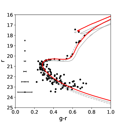
Figure 2.— The observational CMD of Whiting 1, ($g-r$) vs. $r$. Black dots denote the extinction-corrected CMD with stars inside the tidal radius (r${}_{t}<$1$\arcmin$) of Whiting 1. Typical observational error bars are shown at six magnitude levels. Red line denotes our best-CMD fitting with age $\tau$=6.5 Gyr, $z$=0.005, and $\rm d_{\odot}$=26.9 kpc, dashed and solid gray lines denote the model fittings from Carraro et al. (2007) and Valcheva et al. (2015), respectively.

2.3. The orbit of Whiting 1

With help of Gaia EDR3 (Gaia Collaboration et al., 2016, 2021), we are able to compute the orbit of the Whiting 1 cluster. The mean proper motion of the stars within the tidal radius of the cluster is ($\mu_{\alpha}$,$\mu_{\delta}$)=(-0.1,-2.3) mas/year. Together with the sky position, the distance to the Sun, and the radial velocity of -130.6 km^-1, we use the function orbit in Galpy(Bovy, 2015) to trace back the orbit assuming the MWPotential2014 potential (Bovy, 2015). We integrate the orbit back from present to -1.95 Gyr, where 1.95 Gyr is about the simulated orbital period of Whiting 1. The orbit of Whiting 1 is represented by the black solid line in Figure 3, in forms of three coordinate systems. The dots are the simulated Sagittarius Stream stars from Law & Majewski (2010b), with gray for the leading part and blue for trailing part, respectively. It clearly shows that the Whiting 1 orbit is quite consistent with that of the Sagittarius trailing stream in three different coordinate systems. This is not a surprise because, at the sky location ($\alpha$,$\delta$,$\rm d_{\odot}$) of Whiting 1, the observed 3D velocity ($\mu_{\alpha}$,$\mu_{\delta}$,RV) of Whiting 1 is very similar to the observations of the Sgr trailing stream (Antoja et al., 2020; Bellazzini et al., 2020; Carraro et al., 2007; Carballo-Bello et al., 2017). This consistence provides an extra support that Whiting 1 is associated with the Sgr dSph.

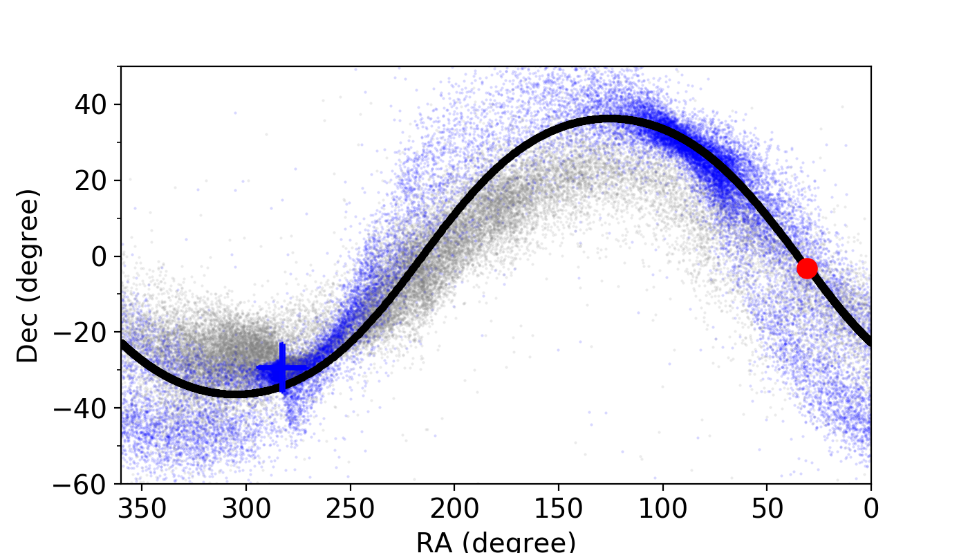
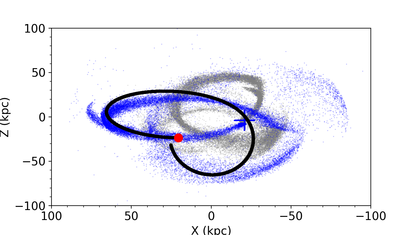
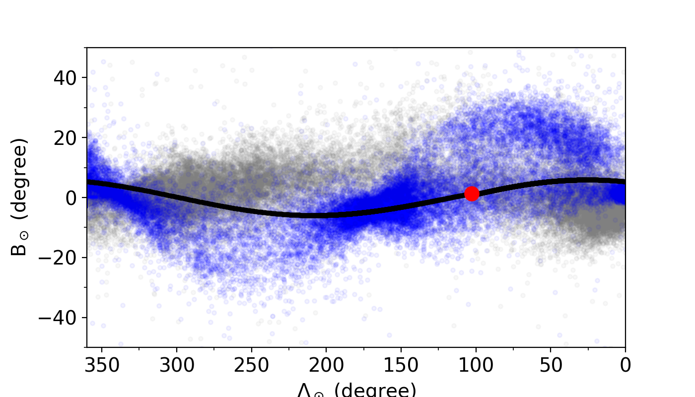
Figure 3.— The orbit of Whiting 1. The top panel shows the orbit in right ascension and declination, the middle panel in Galactic XZ plane, while the bottom panel in a coordinate system ($\Lambda_{\odot}$,B_⊙) aligned with the orbit of Sagittarius, as defined in Majewski et al. (2003). In each panel, red dot denotes the current position of Whiting 1, a solid black line denotes the integrated orbit of Whiting 1 from present back to 1.95 Gyr ago, a blue plus denotes the position of the Sgr dSph, blue and gray dots denote the modeling particles of the Sgr trailing and leading streams from the data of Law & Majewski (2010b).

2.4. Matched filter method

We apply the MF method to search extra-tidal features around Whiting 1. The basic procedures are described in Rockosi et al. (2002). Whiting 1 is embedded in the Sgr trailing stream, so using an optimal CMD template is crucial for this work. To build the filter, we have chosen to use synthetic CMD in $(g-r,r)$, which can utmost avoid the contamination by field objects. We generate the synthetic CMD by using the best-fit isochrone obtained in Section 2.2. We convolve the isochrone with the luminosity function of the cluster and apply the actual photometric uncertainties to the isochrone. No completeness correction is applied for the filter because we only use partial CMD ($r<$22.5 mag) as the MF template. The final CDM filter is shown in Figure 4.

The Galactic background CMD is necessary for the MF method. An adjacent area of the sky is applied, excluding a window around Whiting 1. The four-region background is as shown in Figure 5, with 20^∘$<$RA$<$23^∘, -5^∘$<$Dec$<$0^∘, and 23^∘$<$RA$<$26^∘, -5^∘$<$Dec$<$0^∘, and 34^∘$<$RA$<$37^∘, -5^∘$<$Dec$<$0^∘, and 37^∘$<$RA$<$40^∘, -5^∘$<$Dec$<$0^∘. The average of the $(g-r,r)$ Hess diagrams is defined as the mean background density.

The MF output, $\alpha$, which is defined as the densities of the stars that passed the MF selection, is considered as the final signal of the substructure, as presented in Figure 6.

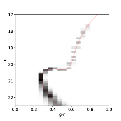
Figure 4.— The synthetic CMD filter for Whiting 1. It was constructed under the the best-fit isochrone from Section 2.2 (red line in the plot), by considering the luminosity function of Whiting 1 and the typical observation errors. The bin size for the x-axis is 0.05 in mag, and the bin size for the y-axis is 0.1 in mag.

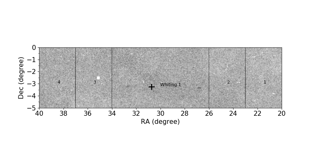
Figure 5.— Figure demonstrates how the Galactic background fields are selected. Fields 1-4 denote the star distribution of the background, defined at the boundaries: 20^∘$<$RA$<$23^∘, 23^∘$<$RA$<$26^∘, 34^∘$<$RA$<$37^∘, 37^∘$<$RA$<$40^∘, and -5^∘$<$Dec$<$0^∘. The small blanks in field 1,2,3 are saturated or crowded areas with no public data. Plus symbol denotes the center of Whiting 1. The very faint diagonal feature around Whiting 1 is the Sgr trailing stream at where the cluster is embedded.

3. Results

3.1. Extra-tidal features around Whiting 1

From the MF output, we obtain the distribution of $\alpha$ over the sky, which is directly relative to the numbers of stars that satisfy the CMD template distribution. Figure 6 shows the logarithm of the density (log${}_{10}\alpha$) centering in Whiting 1, with the left panel for a working field of $10^{\circ}\times 10^{\circ}$ and the right panel for a zoomed-in field of $1.0^{\circ}\times 1.0^{\circ}$. The bin size of the sky is 0.025^∘. The left panel is smoothed by a Gaussian filter with a standard deviation of 1 pixel, while for a detailed view of the real shape of the central feature, no smooth technique is applied to the right panel. At the magnitude limit of $r$=22.5 mag, the survey completeness is 100%, so the density map is not affected by the spatial fluctuation.

For each bin unit of Figure 6, we calculate its significance above the background. The background is at the average level of the field, excluding a window of $0.2^{\circ}\times 0.2^{\circ}$ away from the Whiting 1 center. The background fluctuation is based on the standard deviation of the background region. The significance levels are shown in contour lines in Figure 6, with black for $3.0\sigma$, gray for $4.0\sigma$, and white for $>5.0\sigma$. Since Whiting 1 is a faint and low-mass globular cluster, and it is embedded in the Sgr stream, very low S/N features are possibly not reliable. In this work, we are only care about the features with a significance higher than 3$\sigma$.

From the left panel of Figure 6, we can see many overdense regions spreading over the whole working field. Among them, Whiting 1 is centered in the field. The smoothed density map is easy for searching large-scale features extended from the cluster center, e.g., something like the tidal tails of Palomar 5. However, we could not find any large-scale tidal tails extending from the cluster. Instead, there are many lumpy overdensities arbitrarily distributed all over the map. We have also tried with different bin sizes for the density map, and they come to the same conclusion. So we do not think there is a continuous, long tidal stream for Whiting 1.

For a detailed view of the central feature, we zoom in the field in the right panel, but without smoothing. We see a round-shape feature with the size of a radius of 0.05^∘-0.1^∘ extended from the center of Whiting 1. Note that the tidal radius of Whiting 1 is $r_{t}=$1.0$\arcmin$, but here we detected a much larger size for Whiting 1. Recalling the King-profile fit of the surface density profile of Whiting 1 (Carraro et al., 2007), our detection again suggests there are extra-tidal stars around Whiting 1. From the deep CFHT observations, Muñoz et al. (2018) suggested a tidal radius of 8.4$\arcmin$ for Whiting 1. This confirms a larger size of the cluster. Additionally, we see tiny tails extended from either side of the cluster, which look like the trailing and leading tails of Whiting 1. Together with the central- round feature, the whole structure extends from ($\Delta$RA,$\Delta$Dec)=(0.05, 0.08) to (-0.07, -0.05). By comparing to previous detections of Whiting 1, i.e., detections in Carballo-Bello et al. (2017) and Sollima et al. (2018), our result is consistent with the former detection but a little different to the later one. In fact, if we apply a smooth technique to our raw density map, it presents the same shape as that shown in Carballo-Bello et al. (2017). While to the detection of Sollima et al. (2018), the features of Carballo-Bello et al. (2017) and ours actually cover it: the detection of Sollima et al. (2018) only shows a trailing tail on one side of the cluster, but our detection shows both the leading and trailing tails on opposite sides of the cluster.

We also note that the tails are aligning along the orbital direction of the Sgr orbit as well as that of the Whiting 1 orbit (gray and black arrows in the figure). The mean orbit of the Sgr trailing arm is obtained according to Law & Majewski (2010b) model predictions within the range $0^{\circ}<$RA$<90^{\circ}$. We overplot the Sgr orbit on Whiting 1 by doing a parallel shift. The Whiting 1 orbit is obtained from Section 2.3. From the figure, the consistence between the tails and the orbital directions does not seem to be a coincidence, but is likely to tell a picture of how Whiting 1 was formed: Whiting 1 was originally formed in the Sgr dSph, and it fell into the Milky Way halo in groups, i.e., with dwarf galaxy. By the accretion of the Milky Way, it gradually grew into the current shape with leading and trailing tails on opposite sides of the cluster.

To verify the reality of whole central feature, which is from ($\Delta$RA,$\Delta$Dec)=(0.05, 0.08) to (-0.07, -0.05), we check the density distribution of stars that passed the MF (defined as $\alpha$). The top panels of Figure 7 show the density distribution of Whiting 1-like stars as a function of $\Delta$RA and $\Delta$Dec. It is clearly seen that there is a density enhancement around the center of the cluster. For a significance $>3\sigma$, the width of this overdensity is about 0.1^∘-0.2^∘. This confirms the reality of the central feature. If we excluding the Whiting 1 core stars in the very center, we can still find an overdensity from -0.1^∘ to 0.1^∘ along $\Delta$RA or $\Delta$Dec, which means the $>3\sigma$ overdensity is not only contributed by the core stars of Whiting 1 but also extra-tidal stars of Whiting 1. As the whole central feature aligns along the orbital direction of the Sgr dSph, we did a rotation to make the $x$-axis of the top left panel along the orbital direction of the Sgr dSph, as shown in the bottom left panel of Figure 7. Then we analyze the density distribution of Whiting 1-like stars along the orbital direction of $\Delta\Phi_{1}$ and $\Delta\Phi_{2}$. As expected, we see similar density enhancements along $\Delta\Phi_{1}$ and $\Delta\Phi_{2}$. The width of the overdensity is about 0.1^∘-0.2^∘ for a significance $>3\sigma$. The density distributions of Whiting 1-like stars indicate the reality of the central overdensity.

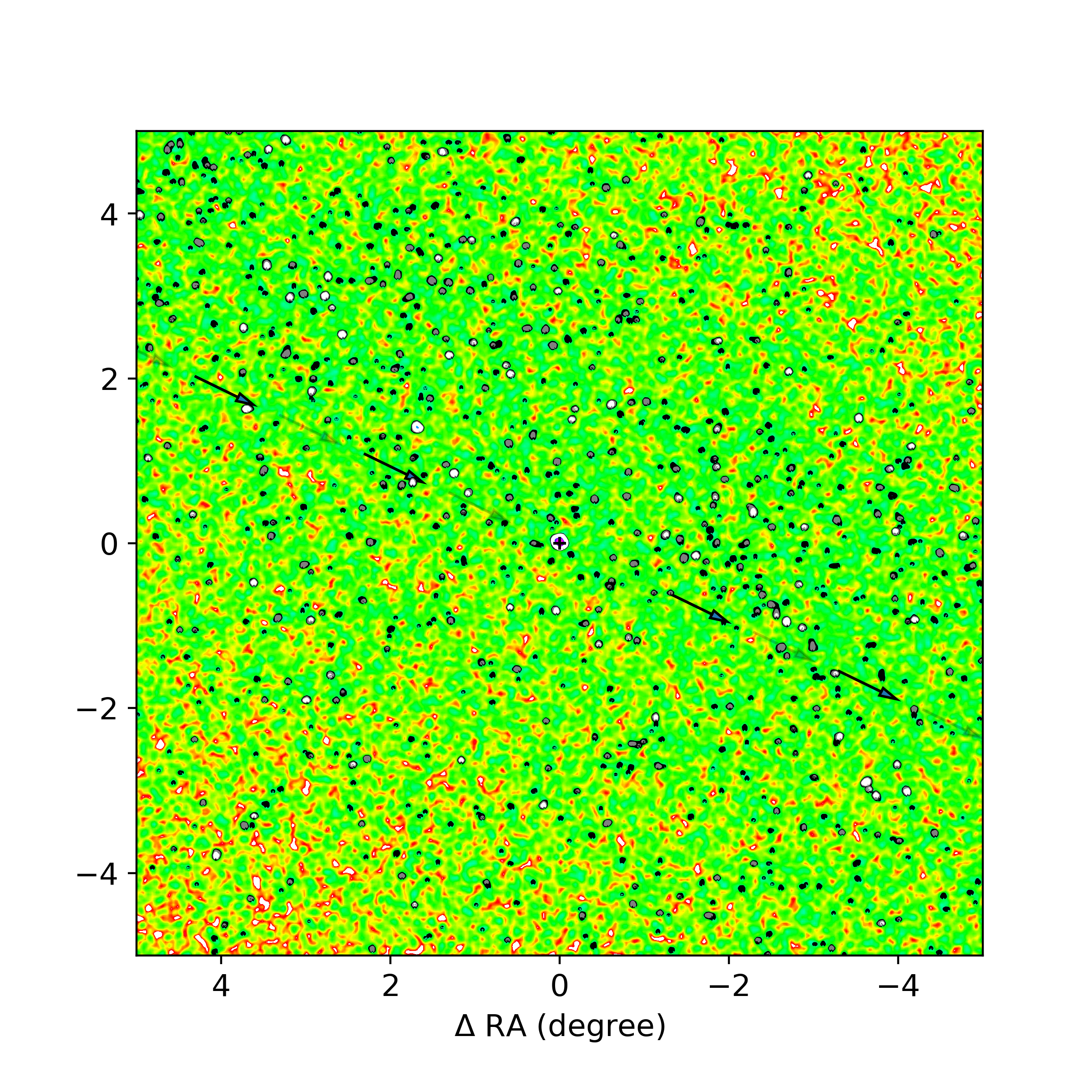
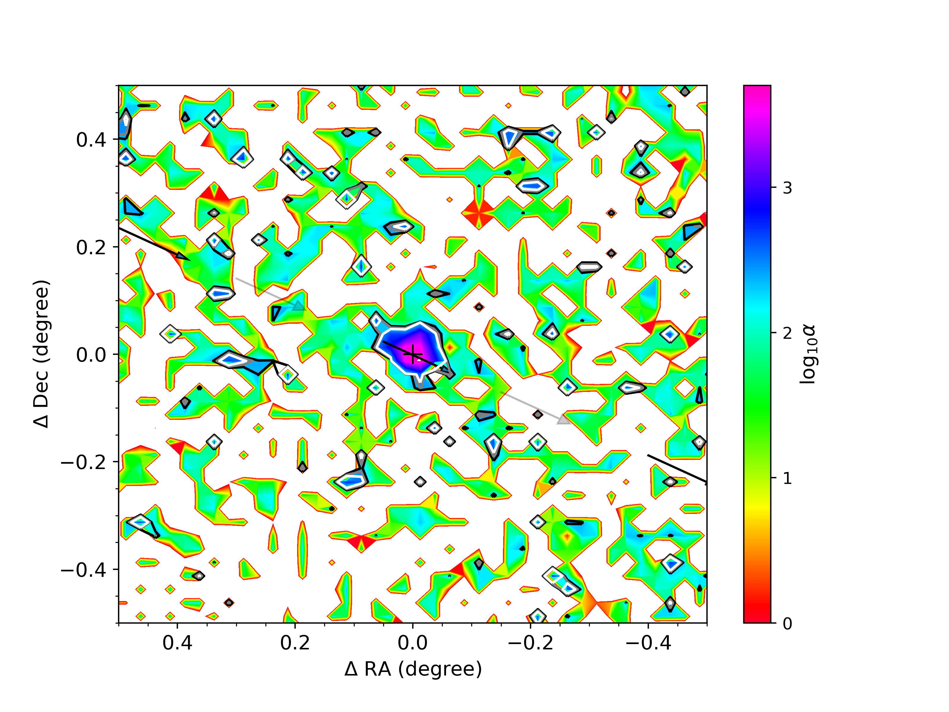
Figure 6.— The Logarithm of the density (log${}_{10}\alpha$) of stars that passed the matched filters $(g-r,r)$. The left panel is a smoothed density map in a field size of $10.0^{\circ}\times 10.0^{\circ}$. The bin size of the density map is 0.025^∘ and the smooth kernel is 1.0 pixel. The right panel is an unsmoothed density map, in a field size of $1.0^{\circ}\times 1.0^{\circ}$. The bin size of the map is the same as that of the left panel. The center of each panel is Whiting 1, as marked with a plus symbol. Color bar indicates the density of MF. Contour lines denote the significance of the detected features, black for $3.0\sigma$, gray for $4.0\sigma$, and white for $>5.0\sigma$. The gray arrow indicates the mean orbital direction of the nearby Sgr trailing stream according to Law & Majewski (2010b). The black arrow indicates the orbit direction of Whiting 1 as shown in Section 2.3.

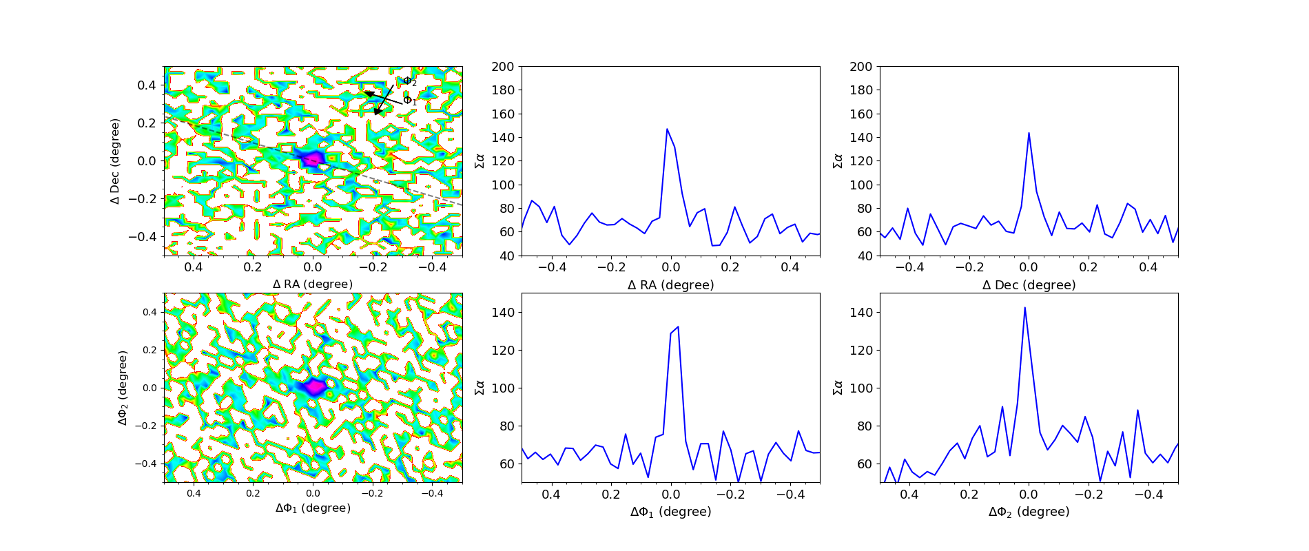
Figure 7.— Top panels: the density distribution of Whiting 1-like stars as a function of $\Delta$RA and $\Delta$Dec. The coordinate reference for $\Delta$RA and $\Delta$Dec is the center of Whiting 1. The density in the middle and right panels is the integrated intense of $\alpha$ along the x-axis. Bottom panels: the same as top panels but as a function of $\Delta\Phi_{1}$ and $\Delta\Phi_{2}$. The coordinate reference for $\Delta\Phi_{1}$ and $\Delta\Phi_{2}$ is the center of Whiting 1. The transformation from (RA,Dec) to ($\Phi_{1}$,$\Phi_{2}$) is indicated in the top left panel. The transformation follows the orbit of Sgr dSph defined in Law & Majewski (2010b).

3.2. The characteristics of the extra-tidal features

The whole view of Whiting 1 structure draws our attention for two reasons:(1) Its size is larger than the cluster core. (2) Its shape is not exactly round; it has tails on opposite directions of the cluster with an elongation aligning along the orbital direction of Whiting 1 as well as the orbital direction of the Sgr trailing stream. We analyze the characteristics of this feature by studying stars inside and outside the structure region.

The left panel of Figure 8 shows how we select the study sample. The red dots in Figure 8 are stars inside the whole feature without any rejections. The gray dots in the figure denote the comparing stars, which are 0.4^∘ away from the Whiting 1 center. We constrain the number of the comparing stars in an annulus with the same number-counts as that of the inside-stars. The black circles in the figure denote the Whiting 1 core stars, which are inside a tidal radius of 1.0$\arcmin$. The middle panel shows the CMD distribution for stars inside and outside the structure. As seen, most (92%) of the inside-stars follow the CMD distribution of the core stars, while only 46% of the outside-stars follow, with the rest of them randomly distributed in the CMD. For the 46% population, most of them are faint stars. Considering the poor accuracy at the faint end, we suggest that the inside-stars are highly Whiting 1 members while the outside-stars are probably from the Sgr trailing stream.

We also tried to study the kinematics of the inside- and outside-stars, however, only 16% of them have velocity data, i.e., proper-motion from Gaia EDR3. In the right panel of Figure 8, we exam the proper-motion distribution of the core stars, and found the core stars roughly follow a distribution with a median of ($\mu_{\alpha}$,$\mu_{\delta}$)= (-0.1,-2.3) mas/year, and a dispersion of 4.0 mas/year. This distribution is close to the proper motion provided by Baumgardt et al. (2019) and Baumgardt & Vasiliev (2021), results of which are based on Gaia DR2 and EDR3. For most of the inside-stars (except three stars marked with blue crosses), they follow the proper-motion distribution of the core stars. While for the outside-stars, a large fraction of them are away from the proper motion clump.

As we know, the Gaia EDR3 proper motion is only accurate down to G=21 mag, so for most of the stars inside or outside the structure, especially the faint stars, their proper motions are not available or have large errors. Owing to this, the right panel cannot tell us the complete proper-motion distribution. We show the proper motion here just for a reference. We need more deep velocity data to study their kinematics. Hopefully, in the future, we can get more velocity data with much deeper spectroscopic surveys, such as the China Space Station Telescope (CSST) and DESI.

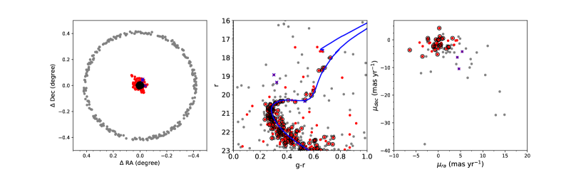
Figure 8.— Left panel: spatial distribution of stars inside and outside the Whiting 1 structure. The coordinate reference is the center of Whiting 1. Red dots denote stars inside the Whiting 1 structure in Figure 6, gray dots denote stars outside the Whiting 1 structure, which are 0.4^∘ away from the Whiting 1 center. The black circles are Whiting 1 core stars. The blue solid line is the Whiting 1 CMD isochrone from Figure 2. Middle panel: the CMD distribution of the stars inside and outside the structure. Right panel: the proper-motion distribution of the stars inside and outside the structure. The proper-motion data are from Gaia EDR3. Only 16% of the inside or outside- stars have proper-motion data, so the distribution is incomplete. The blue crosses denote inside-stars that have proper motion largely away from the proper-motion clump.

3.3. Consider possible contamination to the detection

As we are using the deeper sample from DECaLS DR9, there are many galaxies in the relative sky coverage. To check that the background galaxies are not responsible for our detected substructures, we present their density distribution by using the stellar/galaxy classification provided in DECaLS DR9 catalog, i.e., sources with COMP, DEV,REX, and EXP magnitude types are considered as galaxies. The comparison between the galaxy density distribution and our substructions is presented in the left panel of Figure 9. As seen, no correlation is found between them. Another possible mimic of the substructures is the interstellar extinction. We show the dust map in the right panel of Figure 9. We find that there is no strong correlation between the substructures and the dust map.

In addition, to check the contamination of faint stars, we examine their number- density distribution. We compare the density map of faint stars, i.e., stars with $g$ or $r$ magnitude between 21.5 and 22.5 mag, to our MF detection, and we show the results in the bottom panels of Figure 9. This comparison tells us that the faint stars do contribute to the central feature. However, when we go to a bright-magnitude interval, e.g., $r$ between 19 and 21.5 mag, or other brighter-magnitude intervals, the central structure is still there and shapes the same. This means that the shape and size of the central feature are real, and they are not influenced by the faint stars.

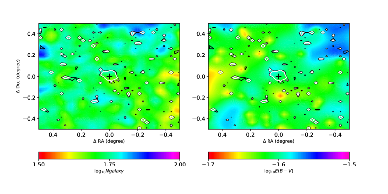
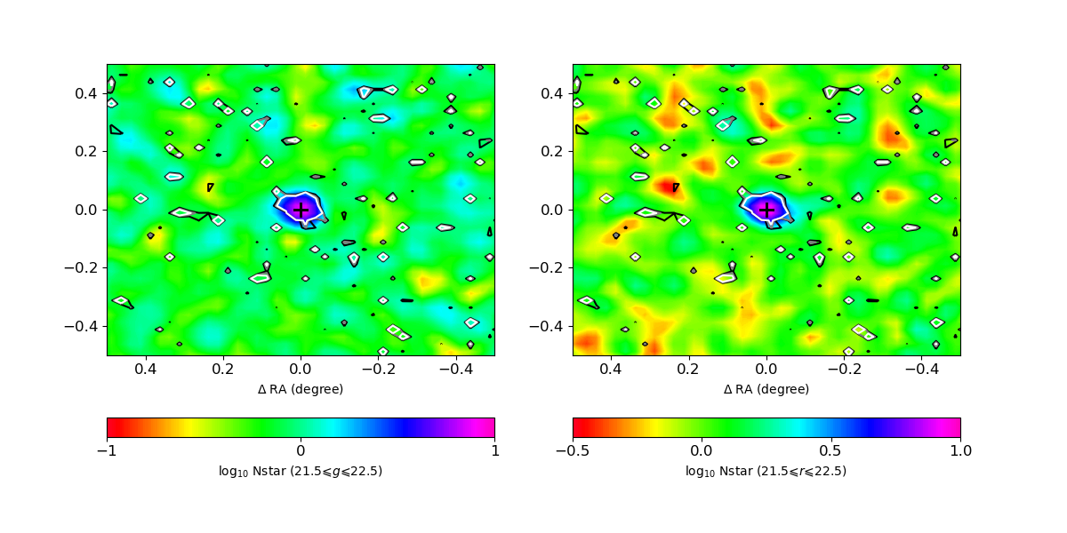
Figure 9.— Top left panel: number-density distribution of the galaxies around Whiting 1. Top right panel: the E(B-V) extinction distribution around Whiting 1. Bottom left and right panels: the number-density distributions for stars in a magnitude interval of 21.5-22.5 mag for $g$ and $r$ bands, respectively. To guide eyes, the MF detections with significance $>3\sigma$ are overplotted with contour lines, with black for 3$\sigma$, gray for 4$\sigma$, white for $>5\sigma$. Pixel scale of the four panels is the same as in Figure 6.

4. Summary

We apply the MF method on the deep survey DECaLS data to search for extra-tidal features around the Whiting 1 cluster. Considering the completeness of the data, we constrain the working sample with $r<=$22.5 mag. Without any smooth technique, we detected a round-shape feature centering in Whiting 1. This central feature has a size in a radius of 0.05^∘-0.1^∘, which gives an area much larger than the Whiting 1 core. Our detection also shows tiny tails in the opposite direction of the central feature, which looks like the leading and trailing tails of Whiting 1. The tails align well along the orbital motion of Whiting 1 and the mean orbital direction of the Sgr trailing stream. To investigate the origin of the whole feature, we checked stars inside the feature with their CMD and proper motions. Most of the stars follow the distributions of the Whiting 1 core stars, which infers that the whole feature possibly belongs to Whiting 1.

The whole view of detected feature is consistent with the detection of Carballo-Bello et al. (2017) and covers the detection of Sollima et al. (2018). Even though we did not find new features compared to the previous study, our detection is the raw density distribution without any smoothing; we can trust on its shape and size. We infer that the detected feature is possibly the true face of Whiting 1 under a depth of $r<22.5$ mag. The morphology of the whole feature seems to suggest that Whiting 1 was initially born in the Sgr dSph, and gradually grew into the current shape by the accretion of the Milky Way. The intriguing origin of Whiting 1 makes it to be a perfect example to study the formation of the Milky Way clusters.

References

- Antoja et al. (2020) Antoja, T., Ramos, P., Mateu, C., et al. 2020, A&A, 635, L3.
- Baumgardt et al. (2019) Baumgardt, H., Hilker, M., Sollima, A., et al. 2019, MNRAS, 482, 5138. doi:10.1093/mnras/sty2997
- Baumgardt & Vasiliev (2021) Baumgardt, H. & Vasiliev, E. 2021, MNRAS, 505, 5957. doi:10.1093/mnras/stab1474
- Bellazzini et al. (2003) Bellazzini, M., Ferraro, F. R., & Ibata, R. 2003, AJ, 125, 188
- Bellazzini et al. (2008) Bellazzini, M., Ibata, R. A., Chapman, S. C., et al. 2008, AJ, 136, 1147
- Bellazzini & Ibata (2018) Bellazzini, M., & Ibata, R. 2018, arXiv:1809.01102
- Bellazzini et al. (2020) Bellazzini, M., Ibata, R., Malhan, K., et al. 2020, A&A, 636, A107.
- Belokurov et al. (2014) Belokurov, V., Koposov, S. E., Evans, N. W., et al. 2014, MNRAS, 437, 116
- Belokurov et al. (2018) Belokurov, V., Erkal, D., Evans, N. W., et al. 2018, MNRAS, 478, 611. doi:10.1093/mnras/sty982
- Bressan et al. (2012) Bressan, A., Marigo, P., Girardi, L., et al. 2012, MNRAS, 427, 127
- Bovy (2015) Bovy, J. 2015, ApJS, 216, 29
- Carraro (2005) Carraro, G. 2005, ApJ, 621, L61
- Carraro et al. (2007) Carraro, G., Zinn, R., & Moni Bidin, C. 2007, A&A, 466, 181
- Carballo-Bello et al. (2014) Carballo-Bello, J. A., Sollima, A., Martínez-Delgado, D., et al. 2014, MNRAS, 445, 2971
- Carballo-Bello et al. (2017) Carballo-Bello, J. A., Corral-Santana, J. M., Martínez-Delgado, D., et al. 2017, MNRAS, 467, L91
- Chen et al. (2014) Chen, Y., Girardi, L., Bressan, A., et al. 2014, MNRAS, 444, 2525
- Chen et al. (2015) Chen, Y., Bressan, A., Girardi, L., et al. 2015, MNRAS, 452, 1068
- Correnti et al. (2010) Correnti, M., Bellazzini, M., Ibata, R. A., Ferraro, F. R., & Varghese, A. 2010, ApJ, 721, 329
- Cui et al. (2012) Cui, X.-Q., Zhao, Y.-H., Chu, Y.-Q., et al. 2012, Research in Astronomy and Astrophysics, 12, 1197
- Dey et al. (2019) Dey, A., Schlegel, D. J., Lang, D., et al. 2019, AJ, 157, 168
- Dinescu et al. (2000) Dinescu, D. I., Majewski, S. R., Girard, T. M., & Cudworth, K. M. 2000, AJ, 120, 1892
- Gaia Collaboration et al. (2016) Gaia Collaboration, Prusti, T., de Bruijne, J. H. J., et al. 2016, A&A, 595, A1
- Gaia Collaboration et al. (2021) Gaia Collaboration, Brown, A. G. A., Vallenari, A., et al. 2021, A&A, 649, A1. doi:10.1051/0004-6361/202039657
- Haywood et al. (2018) Haywood, M., Di Matteo, P., Lehnert, M. D., et al. 2018, ApJ, 863, 113. doi:10.3847/1538-4357/aad235
- Helmi & White (1999a) Helmi, A., & White, S. D. M. 1999a, MNRAS, 307, 495
- Helmi & White (1999b) Helmi, A., & White, S. D. M. 1999b, The Third Stromlo Symposium: The Galactic Halo, 165, 89
- Helmi et al. (1999) Helmi, A., White, S. D. M., de Zeeuw, P. T., & Zhao, H. 1999, Nature, 402, 53
- Helmi et al. (2003) Helmi, A., White, S. D. M., & Springel, V. 2003, MNRAS, 339, 834
- Helmi (2004) Helmi, A. 2004, MNRAS, 351, 643
- Helmi et al. (2018) Helmi, A., Babusiaux, C., Koppelman, H. H., et al. 2018, Nature, 563, 85. doi:10.1038/s41586-018-0625-x
- Ibata et al. (1994) Ibata, R. A., Gilmore, G., & Irwin, M. J. 1994, Nature, 370, 194
- Ibata et al. (2001) Ibata, R., Lewis, G. F., Irwin, M., Totten, E., & Quinn, T. 2001, ApJ, 551, 294
- Ibata et al. (2013) Ibata, R. A., Lewis, G. F., Conn, A. R., et al. 2013, Nature, 493, 62
- Johnston et al. (1996) Johnston, K. V., Hernquist, L., & Bolte, M. 1996, ApJ, 465, 278
- Küpper et al. (2015) Küpper, A. H. W., Balbinot, E., Bonaca, A., et al. 2015, ApJ, 803, 80
- Law et al. (2005) Law, D. R., Johnston, K. V., & Majewski, S. R. 2005, ApJ, 619, 807
- Law & Majewski (2010a) Law, D. R., & Majewski, S. R. 2010a, ApJ, 718, 1128
- Law & Majewski (2010b) Law, D. R., & Majewski, S. R. 2010b, ApJ, 714, 229
- Li et al. (2019) Li, J., FELLOW, . (LAMOST ., Liu, C., et al. 2019, ApJ, 874, 138
- Majewski et al. (2003) Majewski, S. R., Skrutskie, M. F., Weinberg, M. D., & Ostheimer, J. C. 2003, ApJ, 599, 1082
- Marigo et al. (2017) Marigo, P., Girardi, L., Bressan, A., et al. 2017, ApJ, 835, 77
- Martínez-Delgado et al. (2002) Martínez-Delgado, D., Zinn, R., Carrera, R., & Gallart, C. 2002, ApJ, 573, L19
- Massari et al. (2019) Massari, D., Koppelman, H. H., & Helmi, A. 2019, A&A, 630, L4
- Muñoz et al. (2018) Muñoz, R. R., Côté, P., Santana, F. A., et al. 2018, ApJ, 860, 66. doi:10.3847/1538-4357/aac16b
- Myeong et al. (2018) Myeong, G. C., Evans, N. W., Belokurov, V., et al. 2018, ApJ, 856, L26. doi:10.3847/2041-8213/aab613
- Myeong et al. (2019) Myeong, G. C., Vasiliev, E., Iorio, G., et al. 2019, MNRAS, 488, 1235. doi:10.1093/mnras/stz1770
- Pastorelli et al. (2019) Pastorelli, G., Marigo, P., Girardi, L., et al. 2019, MNRAS, 485, 5666
- Rockosi et al. (2002) Rockosi, C. M., Odenkirchen, M., Grebel, E. K., et al. 2002, AJ, 124, 349
- Schlegel et al. (1998) Schlegel, D. J., Finkbeiner, D. P., & Davis, M. 1998, ApJ, 500, 525
- Salpeter (1955) Salpeter, E. E. 1955, ApJ, 121, 161
- Sesar et al. (2017) Sesar, B., Hernitschek, N., Dierickx, M. I. P., Fardal, M. A., & Rix, H.-W. 2017, ApJ, 844, L4
- Shipp et al. (2018) Shipp, N., Drlica-Wagner, A., Balbinot, E., et al. 2018, ApJ, 862, 114. doi:10.3847/1538-4357/aacdab
- Sollima et al. (2018) Sollima, A., Martínez Delgado, D., Muñoz, R. R., et al. 2018, MNRAS, 476, 4814
- Tang et al. (2014) Tang, J., Bressan, A., Rosenfield, P., et al. 2014, MNRAS, 445, 4287
- Valcheva et al. (2015) Valcheva, A. T., Ovcharov, E. P., Lalova, A. D., et al. 2015, MNRAS, 446, 730
- Vasiliev (2019) Vasiliev, E. 2019, MNRAS, 484, 2832. doi:10.1093/mnras/stz171
- Whiting et al. (2002) Whiting, A. B., Hau, G. K. T., & Irwin, M. 2002, ApJS, 141, 123
- Xu et al. (2021) Xu, X., Zou, H., Zhou, X., et al. 2021, AJ, 161, 12.
- Zhao et al. (2012) Zhao, G., Zhao, Y.-H., Chu, Y.-Q., Jing, Y.-P., & Deng, L.-C. 2012, Research in Astronomy and Astrophysics, 12, 723