Bell-type inequalities for systems of relativistic vector bosons

Abstract

We perform a detailed analysis of the possible violation of various Bell-type inequalities for systems of vector boson-antiboson pairs. Considering the general case of an overall scalar state of the bipartite system, we identify two distinct classes of such states, and determine the joint probabilities of spin measurement outcomes for each them. We calculate the expectation values of the CHSH, Mermin and CGLMP inequalities and find that while the generalised CHSH inequality is not expected to be violated for any of the scalar states, in the case of the Mermin and CGLMP inequalities the situation is different – these inequalities can be violated in certain scalar states while they cannot be violated in others. Moreover, the degree of violation depends on the relative speed of the two particles.

1 Introduction

Quantum mechanics predicts that the results of measurements exhibit correlations that differ radically from those of classical physics. Einstein, Podolsky and Rosen were sufficiently disturbed by the apparent lack of realism in quantum measurements, in particular those corresponding to non-commuting operators, that they doubted the completeness of the theory [1]. In response, Bell [2] considered the predictions of theories that are both local (such the physical influences cannot travel faster than the speed of light), and realistic (having physical properties that are independent of observation). He showed that, under certain assumptions, one could perform experimental tests that could distinguish between the predictions of quantum theory and those of such local realistic theories. His method was based on the observation that quantum mechanical predictions for particular correlated expectation values disobey a mathematical inequality – a so-called ‘Bell Inequality’ – that local realistic theories must satisfy.

Subsequent experimental tests of Bell-like inequalities have been performed a variety of physics systems using e.g. photons [3, 4], ions [5], superconducting systems [6] and solid-state systems [7]. More recent examples include so-called ‘loop-hole-free’ tests [8, 9, 10], in which special attention was paid to issues of causality, efficiency and freedom of choice of experimental settings. Bell tests have also been performed experimentally on pairs photons with orbital angular momentum [11], where any measurement of each of the two subsystems results in one of three possible outcomes.

Violation of Bell inequalities by quantum-mechanical probabilities is usually discussed within the framework of non-relativistic quantum mechanics. However, the description of EPR experiments with relativistic particles should be performed in a relativistic setting. Quantum entanglement and Bell inequalities in such a setting have been considered in the literature starting from Czachor’s paper [12]. Since then a large number of papers on the subject have been published, see, e.g., [13, 14, 15, 16, 17, 18, 19, 20, 21, 22, 23, 24, 25, 26, 27, 28, 29, 30] and references therein. It is worth taking note that the description of EPR experiments in a relativistic framework is hindered by theoretical and interpretational difficulties. One of the most important problems is related to the appropriate definition of a relativistic spin operator which is rooted in the non-existence of the Lorentz-covariant position operator in relativistic quantum mechanics [31]. We discuss these issues in more detail in Sec. 3.

In Ref. [21], the EPR correlations in the spins of a pair of identical relativistic spin-1 bosons were considered and the expectation values of various correlators calculated analytically. More recently a proposal was made [32] for testing Bell inequalities using a pair of spin-1 $W^{+}$ and $W^{-}$ bosons resulting from the decay of a spin-0 Higgs boson. Several distinctive features of these recently-proposed measurements make them particularly interesting both in terms of their experimental setup and the interpretation of the results. Firstly, the extremely short (sub-fm) sub-nuclear length scales of the bipartite systems under test are many orders of magnitude shorter than any existing measurements, making this a novel and unexplored regime. Secondly at least one $W$ must be off-mass-shell if produced in a Higgs boson decay, since the mass of the Higgs boson is less than the sum of the $W^{+}$ and $W^{-}$ bosons. This opens the possibility of performing Bell-inequality tests using rather virtual particles, again a regime in which we are not aware of existing tests. Finally, the use of “self-measuring” quantum spin states – which exploit the chiral nature of the weak force to measure the bosons’ spins from the emitted direction of their daughter leptons – challenges the assumption of the experimentalist’s freedom-of-choice that is typically made in Bell tests. These features provide motivation for increasing our understanding Bell-inequality violation in systems of vector bosons, however we do not rely on them in what follows.

2 Scalar states of two vector bosons

We are interested in states containing two relativistic vector bosons, which we label $a$ corresponding to the particle, and $b$ corresponding to its antiparticle. We consider here states that have sharp momentum, and label the four momentum of the particle $k$ and that of the antiparticle $p$. The simplifying assumption of states with sharp momentum allows the study of the relativistic effects without the additional complications associated with finite-width effects.

The method of constructing the corresponding single-particle (and single-anti-particle) states is presented for completeness in Appendices B and C, which themselves further develop the formalism described in Ref. [21]. The result is that a covariant boson-antiboson state corresponding to this situation takes the following form

$$e_{\lambda}^{\mu}(k)e_{\sigma}^{\nu}(p)|(k,\lambda);(p,\sigma)\rangle\equiv e_{\lambda}^{\mu}(k)e_{\sigma}^{\nu}(p)a^{\dagger}_{\lambda}(k)b^{\dagger}_{\sigma}(p)|0\rangle,$$ (1)

where the meanings of the amplitudes $e(k)$ and the creation operators $a^{\dagger},b^{\dagger}$ are as described in Appendix B.

Here we consider a general scalar state in the following form

$$|\alpha(k,p)\rangle=g_{\mu\nu}(k,p)e_{\lambda}^{\mu}(k)e_{\sigma}^{\nu}(p)|(k,\lambda);(p,\sigma)\rangle,$$ (2)

where

$$g_{\mu\nu}(k,p)=\eta_{\mu\nu}+\tfrac{c}{(kp)}\big{(}k_{\mu}p_{\nu}+p_{\mu}k_{\nu}\big{)},\quad c\in{\mathbb{R}}.$$ (3)

We note that transversality condition (60) for amplitudes $e(k)$ reduces the second term in the bracket in (3) to the $p_{\mu}k_{\nu}$ only. Choosing the above parametrization we exclude from our considerations the state $p_{\mu}k_{\nu}e_{\lambda}^{\mu}(k)e_{\sigma}^{\nu}(p)|(k,\lambda);(p,\sigma)\rangle$. However, this state is separable.

The scalar state defined in Eq. (2) is normalized as follows

$$\langle\alpha(k,p)|\alpha(k,p)\rangle=4k^{0}p^{0}(\delta^{3}(\textbf{0}))^{2}A(k,p),$$ (4)

with

$$A(k,p)=2+\Big{[}c\tfrac{m^{2}}{(kp)}-\tfrac{(kp)}{m^{2}}(1+c)\Big{]}^{2}.$$ (5)

Eq. (2) defines a whole variety of scalar states, two of which are distinguished.

The first one, $|\psi(k,p)\rangle$, corresponds to the choice $c_{\psi}=0$:

$$|\psi(k,p)\rangle=\eta_{\mu\nu}e_{\lambda}^{\mu}(k)e_{\sigma}^{\nu}(p)|(k,\lambda);(p,\sigma)\rangle.$$ (6)

It is the simplest and the most natural scalar state. In [21] we considered the Einstein–Podolsky-Rosen type experiment with two bosons in the state $|\psi(k,p)\rangle$. The normalization factor $A(k,p)$ of the state $|\psi(k,p)\rangle$ has the simple form

$$A^{\psi}(k,p)=2+\tfrac{(kp)^{2}}{m^{4}}.$$ (7)

The second interesting scalar state, $|\xi(k,p)\rangle$, corresponds to the choice $c_{\xi}=-1$:

$$|\xi(k,p)\rangle=\Big{(}\eta_{\mu\nu}-\tfrac{1}{(kp)}p_{\mu}k_{\nu}\Big{)}e_{\lambda}^{\mu}(k)e_{\sigma}^{\nu}(p)|(k,\lambda);(p,\sigma)\rangle.$$ (8)

The state $|\xi(k,p)\rangle$ has the property that in the massless limit it converges to a scalar two-photon state. This question was discussed in detail in [37]. Notice also that the normalization factor $A(k,p)$ of the state $|\xi(k,p)\rangle$ also takes the simple form

$$A^{\xi}(k,p)=2+\tfrac{m^{4}}{(kp)^{2}}.$$ (9)

3 Spin operator for a relativistic particle

When we want to calculate explicitly correlation functions, we need to introduce the spin operator for relativistic massive particles. The choice of such an operator is not a trivial problem. We know that in the carrier space of a unitary representation of the Poincaré group there exists a well-defined square of the spin operator

$$\hat{\vec{S}}^{2}=s(s+1)I=-\frac{W^{\mu}W_{\mu}}{m^{2}},$$ (10)

where $s$ denotes spin of a particle and

$$\hat{W}^{\mu}=\tfrac{1}{2}\epsilon^{\mu\nu\gamma\delta}\hat{P}_{\nu}\hat{J}_{\gamma\delta}$$ (11)

is the Pauli-Lubanski four-vector, $\hat{P}_{\nu}$ is the four-momentum operator, $\hat{J}_{\mu\nu}$ denote the generators of the Lorentz group such that $U(\Lambda)=\exp(i\omega^{\mu\nu}\hat{J}_{\mu\nu})$, and we assume $\epsilon^{0123}=1$. On the other hand, spin can be defined as a difference between total angular momentum and the orbital angular momentum $\hat{\vec{L}}=\hat{\vec{Q}}\times\hat{\vec{P}}$:

$$\hat{\vec{S}}=\hat{\vec{J}}-\hat{\vec{Q}}\times\hat{\vec{P}}.$$ (12)

Total angular momentum $\hat{\vec{J}}$ is well defined as the generator of the rotations, $\hat{J}^{i}=\varepsilon^{ijk}\hat{J}^{jk}$, and the momentum operator $\hat{\vec{P}}$ is also well defined (compare Eq. (53)), but there does not exist a generally accepted position operator $\hat{\vec{Q}}$[31]. Different choices of the position operator $\hat{\vec{Q}}$ lead to different spin operators. The most popular position operator was introduced by Newton and Wigner[38]

$$\hat{\vec{Q}}_{NW}=-\frac{1}{2}\Big{[}\frac{1}{\hat{P}^{0}}\hat{\textbf{K}}+\hat{\textbf{K}}\frac{1}{\hat{P}^{0}}\Big{]}-\frac{\hat{\textbf{P}}\times\hat{\textbf{W}}}{m\hat{P}^{0}(m+\hat{P}^{0})},$$ (13)

where $\hat{\vec{K}}$ denotes the boost generators, $\textbf{K}^{i}=\textbf{J}^{0i}$. The Newton-Wigner position operator possesses many desirable properties: it is a vector with commuting, self-adjoint components and it is defined for arbitrary spin. Unfortunately, $\hat{\vec{Q}}_{NW}$ does not transform in a manifestly covariant way under Lorentz boosts.

The spin operator related to the Newton-Wigner position operator is equal to

$$\hat{\textbf{S}}=\frac{1}{m}\Big{(}\hat{\textbf{W}}-\hat{W}^{0}\frac{\hat{\vec{P}}}{\hat{P}^{0}+m}\Big{)}.$$ (14)

This operator has several desirable features. Components of this operator satisfy the standard su(2) Lie algebra commutation relations. Moreover, the square of the operator (14) in a unitary irreducible representation of the Poincaré group is equal to (10). What more, the operator (14) is the only axial vector which is a linear function of the Pauli-Lubanski four-vector components[39]. Finally, as was shown in [40], the operator $\hat{\textbf{S}}$ has an elegant transformation formula $\hat{\textbf{S}}^{\prime}=R(\Lambda,\hat{P})\hat{\textbf{S}}$ under Lorentz group action, where $R(\Lambda,\hat{P})$ is the corresponding Wigner rotation while $\hat{P}$ is the four-momentum operator. That is why in our opinion the spin operator (14) is the most appropriate one and we chose it for our calculations (compare [41]).

The influence of the Newton-Wigner localization of a particle inside a detector during spin measurement on relativistic quantum correlations, but in a case of a fermion pair, was considered in [26]. In Appendix D we have shortly recalled these results adapting them to a system of vector bosons. We concluded there that for real, massive particles there is no problem with localization of a particle inside the detector in situation in which it is directly detected. The extent to which such arguments might also be relevant to measurements of gauge boson spin via the kinematics of their chiral decays, as was used e.g. in [32], is a more involved question, and lies beyond the scope of the present paper.

We note that other spin operators have been also used in the description of relativistic EPR experiments, the most popular one is the operator used by Czachor[12]. This operator is related with the so-called center of mass position operator which has non-commuting components. For more exhaustive discussion of the problem of choice of the proper relativistic spin operator see, e.g., [42, 19, 20, 41, 43, 44, 45, 46, 47, 48].

The spin operator $\hat{\textbf{S}}$ (14) acts on one-particle states according to

$$\hat{\textbf{S}}|k,\sigma\rangle=\textbf{S}_{\lambda\sigma}|k,\lambda\rangle,$$ (15)

where $S^{i}$ are standard spin-1 matrices (compare, e.g., [49]):

$$S^{1}=\tfrac{1}{\sqrt{2}}\begin{pmatrix}0&1&0\\ 1&0&1\\ 0&1&0\\ \end{pmatrix},\quad S^{2}=\tfrac{i}{\sqrt{2}}\begin{pmatrix}0&-1&0\\ 1&0&-1\\ 0&1&0\\ \end{pmatrix},$$ (16)

$$S^{3}=\begin{pmatrix}1&0&0\\ 0&0&0\\ 0&0&-1\\ \end{pmatrix}.$$ (17)

An operator which acts like a spin on particles whose momenta belong to some definite region $\Omega$ in momentum space and gives 0 otherwise has the form

$$\hat{\textbf{S}}^{a}_{\Omega}=\int_{\Omega}\tfrac{d^{3}\textbf{k}}{2k^{0}}a^{\dagger}(k)\textbf{S}a(k),$$ (18)

where $a(k)=\big{(}a_{+1}(k),a_{0}(k),a_{-1}(k)\big{)}^{T}$. A similar operator but acting on antiparticles has the form

$$\hat{\textbf{S}}^{b}_{\Omega}=\int_{\Omega}\tfrac{d^{3}\textbf{k}}{2k^{0}}b^{\dagger}(k)\textbf{S}b(k).$$ (19)

We have

$$\hat{\textbf{S}}^{a}_{\Omega}|(k,\lambda)_{a};(p,\sigma)_{b}\rangle=\chi_{\Omega}(k)\textbf{S}_{\lambda^{\prime}\lambda}|(k,\lambda^{\prime})_{a};(p,\sigma)_{b}\rangle$$ (20)

and

$$\hat{\textbf{S}}^{b}_{\Omega}|(k,\lambda)_{a};(p,\sigma)_{b}\rangle=\chi_{\Omega}(p)\textbf{S}_{\sigma^{\prime}\sigma}|(k,\lambda)_{a};(p,\sigma^{\prime})_{b}\rangle,$$ (21)

where $\chi_{\Omega}$ denotes the characteristic function of the set $\Omega$: $\chi_{\Omega}(k)=1$ for $k\in\Omega$ and $\chi_{\Omega}(k)=0$ for $k\not\in\Omega$. The spectral decomposition of the operator $\boldsymbol{\omega}\cdot\hat{\textbf{S}}^{a}_{\Omega}$ can be written as

$$\boldsymbol{\omega}\cdot\hat{\textbf{S}}^{a}_{\Omega}=1\cdot\Pi^{a+}_{\Omega\boldsymbol{\omega}}+(-1)\cdot\Pi^{a-}_{\Omega\boldsymbol{\omega}}+0\cdot\Pi^{a0}_{\Omega\boldsymbol{\omega}},$$ (22)

where the projectors act in the following way:

$$\Pi^{a\pm}_{\Omega\boldsymbol{\omega}}|(k,\lambda)_{a};(p,\sigma)_{b}\rangle=\\ \tfrac{1}{2}\chi_{\Omega}(k)\Big{(}(\boldsymbol{\omega}\cdot\textbf{S})^{2}_{\lambda^{\prime}\lambda}\pm(\boldsymbol{\omega}\cdot\textbf{S})_{\lambda^{\prime}\lambda}\Big{)}|(k,\lambda^{\prime})_{a};(p,\sigma)_{b}\rangle,$$ (23)

$$\Pi^{a0}_{\Omega\boldsymbol{\omega}}|(k,\lambda)_{a};(p,\sigma)_{b}\rangle=\\ \chi_{\Omega}(k)\Big{(}\delta_{\lambda^{\prime}\lambda}-(\boldsymbol{\omega}\cdot\textbf{S})^{2}_{\lambda^{\prime}\lambda}\Big{)}|(k,\lambda^{\prime})_{a};(p,\sigma)_{b}\rangle.$$ (24)

Analogous formulas can easily be found for $\boldsymbol{\omega}\cdot\hat{\textbf{S}}^{b}_{\Omega}$.

4 Probabilities

Now, let two distant observers, Alice and Bob, be at rest with respect to a given inertial frame and share a pair of bosons in the scalar state $|\alpha(k,p)\rangle$ (Eq. (2)). The probability that Alice obtains $\sigma$ and Bob $\lambda$ ($\lambda,\sigma\in\{-1,0,1\}$), when measuring spin projections on the directions a and b, respectively, are given by the formula

$$P_{\sigma\lambda}=\frac{\langle\alpha(k,p)|\hat{\Pi}_{A\textbf{a}}^{\sigma}\hat{\Pi}_{B\textbf{b}}^{\lambda}|\alpha(k,p)\rangle}{\langle\alpha(k,p)|\alpha(k,p)\rangle}.$$ (25)

Here we assume that Alice (Bob) can register only particles (antiparticles) whose momenta belong to the region $A$ ($B$) in the momentum space and that they use the spin operator given in Eq. (14). Projectors in the above formula are defined in Eqs. (23,24). Further, assuming that Alice can measure only bosons with four-momentum $k$ and Bob those with four-momentum $p$ we find

$$P_{\pm\pm}=\frac{1}{4A(k,p)}\operatorname{Tr}\{M(k,\textbf{a})g(k,p)M(p,\textbf{b})g(k,p)^{T}\\ -N(k,\textbf{a})g(k,p)N(p,\textbf{b})g(k,p)^{T}\},$$ (26a)

$$P_{\pm\mp}=\frac{1}{4A(k,p)}\operatorname{Tr}\{M(k,\textbf{a})g(k,p)M(p,\textbf{b})g(k,p)^{T}\\ +N(k,\textbf{a})g(k,p)N(p,\textbf{b})g(k,p)^{T}\},$$ (26b)

$$P_{0\pm}=\frac{1}{2A(k,p)}\operatorname{Tr}\{T(k,\textbf{a})g(k,p)M(p,\textbf{b})g(k,p)^{T}\},$$ (26c)

$$P_{\pm 0}=\frac{1}{2A(k,p)}\operatorname{Tr}\{M(k,\textbf{a})g(k,p)T(p,\textbf{b})g(k,p)^{T}\},$$ (26d)

$$P_{00}=\frac{1}{A(k,p)}\operatorname{Tr}\{T(k,\textbf{a})g(k,p)T(p,\textbf{b})g(k,p)^{T}\},$$ (26e)

where

$$g(k,p)=[g_{\mu\nu}(k,p)]$$ (27)

and where we have introduced the following notation

$$M(q,\boldsymbol{\omega})=[M(q,\boldsymbol{\omega})^{\mu\nu}]=e^{*\mu}_{\lambda}(q)(\boldsymbol{\omega}\cdot\textbf{S})^{2}_{\lambda\sigma}e^{\nu}_{\sigma}(q),$$ (28)

$$N(q,\boldsymbol{\omega})=[N(q,\boldsymbol{\omega})^{\mu\nu}]=e^{*\mu}_{\lambda}(q)(\boldsymbol{\omega}\cdot\textbf{S})_{\lambda\sigma}e^{\nu}_{\sigma}(q),$$ (29)

$$T(q,\boldsymbol{\omega})=[T(q,\boldsymbol{\omega})^{\mu\nu}]=e^{*\mu}_{\lambda}(q)\big{(}\delta_{\lambda\sigma}-(\boldsymbol{\omega}\cdot\textbf{S})^{2}_{\lambda\sigma}\big{)}e^{\nu}_{\sigma}(q).$$ (30)

With the help of the above formulas one can find $P_{\lambda\sigma}$ for arbitrary $k$ and $p$. However, the resulting formulas are complicated. Thus, here we restrict ourselves to the situation when Alice and Bob’s frame coincides with the center of mass frame of the boson pair ($p=k^{\pi}=(k^{0},-\textbf{k})$). Let us introduce the notation

$$x=\tfrac{\textbf{k}^{2}}{m^{2}},\quad\textbf{n}=\tfrac{\textbf{k}}{|\textbf{k}|}.$$ (31)

Using this notation we have in the center of mass frame

$$A(k,k^{\pi})=2+\tfrac{[4x(x+1)(c+1)+1]^{2}}{(2x+1)^{2}}$$ (32)

and

$$P_{\pm\pm}=\frac{1}{4A(k,k^{\pi})}\Big{\{}1+4x(x+1)\big{(}1+2c\tfrac{x}{2x+1}\big{)}\big{(}1+2c\tfrac{x+1}{2x+1}\big{)}\big{[}1-(\textbf{a}\cdot\textbf{n})^{2}-(\textbf{b}\cdot\textbf{n})^{2}\big{]}+\Big{[}(\textbf{a}\cdot\textbf{b})+2x\big{(}1+2c\tfrac{x+1}{2x+1}\big{)}(\textbf{a}\cdot\textbf{n})(\textbf{b}\cdot\textbf{n})\Big{]}^{2}\\ -2\Big{[}(\textbf{a}\cdot\textbf{b})+2x\big{(}1+2c\tfrac{x+1}{2x+1}\big{)}\big{[}(\textbf{a}\cdot\textbf{b})-(\textbf{a}\cdot\textbf{n})(\textbf{b}\cdot\textbf{n})\big{]}\Big{]}\Big{\}},$$ (33a)

$$P_{\pm\mp}=\frac{1}{4A(k,k^{\pi})}\Big{\{}1+4x(x+1)\big{(}1+2c\tfrac{x}{2x+1}\big{)}\big{(}1+2c\tfrac{x+1}{2x+1}\big{)}\big{[}1-(\textbf{a}\cdot\textbf{n})^{2}-(\textbf{b}\cdot\textbf{n})^{2}\big{]}+\Big{[}(\textbf{a}\cdot\textbf{b})+2x\big{(}1+2c\tfrac{x+1}{2x+1}\big{)}(\textbf{a}\cdot\textbf{n})(\textbf{b}\cdot\textbf{n})\Big{]}^{2}\\ +2\Big{[}(\textbf{a}\cdot\textbf{b})+2x\big{(}1+2c\tfrac{x+1}{2x+1}\big{)}\big{[}(\textbf{a}\cdot\textbf{b})-(\textbf{a}\cdot\textbf{n})(\textbf{b}\cdot\textbf{n})\big{]}\Big{]}\Big{\}},$$ (33b)

$$P_{0\pm}=\frac{1}{2A(k,k^{\pi})}\Big{\{}1+4x(x+1)\big{(}1+2c\tfrac{x}{2x+1}\big{)}\big{(}1+2c\tfrac{x+1}{2x+1}\big{)}(\textbf{a}\cdot\textbf{n})^{2}-\Big{[}(\textbf{a}\cdot\textbf{b})+2x\big{(}1+2c\tfrac{x+1}{2x+1}\big{)}(\textbf{a}\cdot\textbf{n})(\textbf{b}\cdot\textbf{n})\Big{]}^{2}\Big{\}},$$ (33c)

$$P_{\pm 0}=\frac{1}{2A(k,k^{\pi})}\Big{\{}1+4x(x+1)\big{(}1+2c\tfrac{x}{2x+1}\big{)}\big{(}1+2c\tfrac{x+1}{2x+1}\big{)}(\textbf{b}\cdot\textbf{n})^{2}-\Big{[}(\textbf{a}\cdot\textbf{b})+2x\big{(}1+2c\tfrac{x+1}{2x+1}\big{)}(\textbf{a}\cdot\textbf{n})(\textbf{b}\cdot\textbf{n})\Big{]}^{2}\Big{\}},$$ (33d)

$$P_{00}=\frac{1}{A(k,k^{\pi})}\Big{[}(\textbf{a}\cdot\textbf{b})+2x\big{(}1+2c\tfrac{x+1}{2x+1}\big{)}(\textbf{a}\cdot\textbf{n})(\textbf{b}\cdot\textbf{n})\Big{]}^{2}.$$ (33e)

The correlation function defined as

$$C(\textbf{a},k;\textbf{b},k^{\pi}) =\sum_{\lambda,\sigma=-1,0,1}\lambda\sigma P_{\lambda\sigma}=2(P_{\pm\pm}-P_{\pm\mp})$$ (34)

is equal to

$$C(\textbf{a},k;\textbf{b},k^{\pi})=-\tfrac{2}{A(k,k^{\pi})}\Big{[}(\textbf{a}\cdot\textbf{b})\\ +2x\big{(}1+2c\tfrac{x+1}{2x+1}\big{)}\Big{(}(\textbf{a}\cdot\textbf{b})-(\textbf{a}\cdot\textbf{n})(\textbf{b}\cdot\textbf{n})\Big{)}\Big{]}.$$ (35)

Let us now consider the nonrelativistic and ultrarelativistic limits of the above probabilities.

4.0.1 Nonrelativistic limit

In the nonrelativistic limit ($x\to 0$) we obtain

$$P_{\pm\pm}(x\to 0)=\tfrac{1}{12}[1-(\textbf{a}\cdot\textbf{b})]^{2},$$ (36a)

$$P_{\pm\mp}(x\to 0)=\tfrac{1}{12}[1+(\textbf{a}\cdot\textbf{b})]^{2},$$ (36b)

$$P_{0\pm}(x\to 0)=P_{\pm 0}(x\to 0)=\tfrac{1}{6}[1-(\textbf{a}\cdot\textbf{b})^{2}],$$ (36c)

$$P_{00}(x\to 0)=\tfrac{1}{3}(\textbf{a}\cdot\textbf{b})^{2}.$$ (36d)

These probabilities are the same as those calculated in the framework of nonrelativistic quantum mechanics in the singlet spin-1 state

$$|\Psi^{\mathrm{nonrel}}_{\mathrm{singlet}}\rangle=\tfrac{1}{\sqrt{3}}\big{(}|1\rangle|-1\rangle-|0\rangle|0\rangle+|-1\rangle|1\rangle\big{)}.$$ (37)

4.0.2 Ultrarelativistic limit

In the ultrarelativistic limit ($x\to\infty$) we have to distinguish two separate cases: $c=-1$, corresponding to the state $|\xi\rangle$, and $c\not=-1$ which contains the state $|\psi\rangle$.

In the case $c\not=-1$ we get

$$P^{c\not=-1}_{\pm\pm}(x\to\infty)=P^{c\not=-1}_{\pm\mp}(x\to\infty)\\ =\tfrac{1}{4}\big{[}1-(\textbf{a}\cdot\textbf{n})^{2}\big{]}\big{[}1-(\textbf{b}\cdot\textbf{n})^{2}\big{]},$$ (38a)

$$P^{c\not=-1}_{0\pm}(x\to\infty)=\tfrac{1}{2}(\textbf{a}\cdot\textbf{n})^{2}\big{[}1-(\textbf{b}\cdot\textbf{n})^{2}\big{]},$$ (38b)

$$P^{c\not=-1}_{\pm 0}(x\to\infty)=\tfrac{1}{2}(\textbf{b}\cdot\textbf{n})^{2}\big{[}1-(\textbf{a}\cdot\textbf{n})^{2}\big{]},$$ (38c)

$$P^{c\not=-1}_{00}(x\to\infty)=(\textbf{a}\cdot\textbf{n})^{2}(\textbf{b}\cdot\textbf{n})^{2}.$$ (38d)

The correlation function in this case vanishes

$$C^{c\not=-1}(\textbf{a},k;\textbf{b},k^{\pi},x\to\infty)=0.$$ (39)

The case $c\not=-1$ includes the state $|\psi(k,k^{\pi})\rangle$. The probabilities in the ultrarelativistic limit in this state were given in Eq. (60) in Ref. [21] and they coincide with the above formulas.

The case $c=-1$ corresponds to the state $|\xi(k,k^{\pi})\rangle$ and for this state we obtain

$$P^{\xi}_{\pm\pm}(x\to\infty)=\tfrac{1}{8}\big{\{}\big{[}(\textbf{a}\cdot\textbf{b})-(\textbf{a}\cdot\textbf{n})(\textbf{b}\cdot\textbf{n})\big{]}^{2}\\ +\big{[}(\textbf{a}\cdot\textbf{n})-(\textbf{b}\cdot\textbf{n})\big{]}^{2}\big{\}},$$ (40a)

$$P^{\xi}_{\pm\mp}(x\to\infty)=\tfrac{1}{8}\big{\{}\big{[}(\textbf{a}\cdot\textbf{b})-(\textbf{a}\cdot\textbf{n})(\textbf{b}\cdot\textbf{n})\big{]}^{2}\\ +\big{[}(\textbf{a}\cdot\textbf{n})+(\textbf{b}\cdot\textbf{n})\big{]}^{2}\big{\}},$$ (40b)

$$P^{\xi}_{0\mp}(x\to\infty)=\tfrac{1}{4}\big{\{}1-(\textbf{a}\cdot\textbf{n})^{2}\\ -\big{[}(\textbf{a}\cdot\textbf{b})-(\textbf{a}\cdot\textbf{n})(\textbf{b}\cdot\textbf{n})\big{]}^{2}\big{\}},$$ (40c)

$$P^{\xi}_{\mp 0}(x\to\infty)=\tfrac{1}{4}\big{\{}1-(\textbf{b}\cdot\textbf{n})^{2}\\ -\big{[}(\textbf{a}\cdot\textbf{b})-(\textbf{a}\cdot\textbf{n})(\textbf{b}\cdot\textbf{n})\big{]}^{2}\big{\}},$$ (40d)

$$P^{\xi}_{00}(x\to\infty)=\tfrac{1}{2}\big{[}(\textbf{a}\cdot\textbf{b})-(\textbf{a}\cdot\textbf{n})(\textbf{b}\cdot\textbf{n})\big{]}^{2},$$ (40e)

while the correlation function is equal to

$$C^{\xi}(\textbf{a},k;\textbf{b},k^{\pi},x\to\infty)=-(\textbf{a}\cdot\textbf{n})(\textbf{b}\cdot\textbf{n}).$$ (41)

It is interesting to observe that the state $|\xi(k,k^{\pi})\rangle$ is distinguished by the property that for this state only the correlation function does not vanish in the ultrarelativistic limit.

In the following we concentrate on the most interesting (and natural) states $|\psi\rangle$ and $|\xi\rangle$.

4.0.3 Probabilities in the state $|\psi(k,k^{\pi})\rangle$

We have calculated these probabilities in our previous paper [21], they are given by Eq. (58) from [21]. For convenience we recall them here

$$P^{\psi}_{\pm\pm}=\tfrac{1}{4[(2x+1)^{2}+2]}\big{\{}(2x+1)^{2}-2(2x+1)(\textbf{a}\cdot\textbf{b})\\ +4x(\textbf{a}\cdot\textbf{n})(\textbf{b}\cdot\textbf{n})-4x(x+1)\big{[}(\textbf{a}\cdot\textbf{n})^{2}+(\textbf{b}\cdot\textbf{n})^{2}\big{]}\\ +\big{[}(\textbf{a}\cdot\textbf{b})+2x(\textbf{a}\cdot\textbf{n})(\textbf{b}\cdot\textbf{n})\big{]}^{2}\big{\}},$$ (42a)

$$P^{\psi}_{\pm\mp}=\tfrac{1}{4[(2x+1)^{2}+2]}\big{\{}(2x+1)^{2}+2(2x+1)(\textbf{a}\cdot\textbf{b})\\ -4x(\textbf{a}\cdot\textbf{n})(\textbf{b}\cdot\textbf{n})-4x(x+1)\big{[}(\textbf{a}\cdot\textbf{n})^{2}+(\textbf{b}\cdot\textbf{n})^{2}\big{]}\\ +\big{[}(\textbf{a}\cdot\textbf{b})+2x(\textbf{a}\cdot\textbf{n})(\textbf{b}\cdot\textbf{n})\big{]}^{2}\big{\}},$$ (42b)

$$P^{\psi}_{0\mp}=\tfrac{1}{2[(2x+1)^{2}+2]}\big{\{}1+4x(x+1)(\textbf{a}\cdot\textbf{n})^{2}\\ -\big{[}(\textbf{a}\cdot\textbf{b})+2x(\textbf{a}\cdot\textbf{n})(\textbf{b}\cdot\textbf{n})\big{]}^{2}\big{\}},$$ (42c)

$$P^{\psi}_{\mp 0}=\tfrac{1}{2[(2x+1)^{2}+2]}\big{\{}1+4x(x+1)(\textbf{b}\cdot\textbf{n})^{2}\\ -\big{[}(\textbf{a}\cdot\textbf{b})+2x(\textbf{a}\cdot\textbf{n})(\textbf{b}\cdot\textbf{n})\big{]}^{2}\big{\}},$$ (42d)

$$P^{\psi}_{00}=\tfrac{1}{(2x+1)^{2}+2}\big{[}(\textbf{a}\cdot\textbf{b})+2x(\textbf{a}\cdot\textbf{n})(\textbf{b}\cdot\textbf{n})\big{]}^{2}.$$ (42e)

The correlation function for the state $|\psi(k,k^{\pi})\rangle$ was given in Eq. (59) in [21] and reads

$$C^{\psi}(\textbf{a},k;\textbf{b},k^{\pi})=\tfrac{-2}{(2x+1)^{2}+2}\big{[}(2x+1)(\textbf{a}\cdot\textbf{b})\\ -2x(\textbf{a}\cdot\textbf{n})(\textbf{b}\cdot\textbf{n})\big{]}.$$ (43)

4.0.4 Probabilities in the state $|\xi(k,k^{\pi})\rangle$

In this case we insert into Eq. (33) the following values:

$$c_{\xi}=-1,\quad A^{\xi}(k,k^{\pi})=2+\tfrac{1}{(2x+1)^{2}}.$$ (44)

The resulting probabilities have the following form

$$P^{\xi}_{\pm\pm}=\tfrac{1}{4[2(2x+1)^{2}+1]}\big{\{}\big{[}(2x+1)(\textbf{a}\cdot\textbf{b})-2x(\textbf{a}\cdot\textbf{n})(\textbf{b}\cdot\textbf{n})\big{]}^{2}\\ +(2x+1)^{2}-4x(x+1)\big{[}1-(\textbf{a}\cdot\textbf{n})^{2}-(\textbf{b}\cdot\textbf{n})^{2}\big{]}\\ -2(2x+1)\big{[}(\textbf{a}\cdot\textbf{b})+2x(\textbf{a}\cdot\textbf{n})(\textbf{b}\cdot\textbf{n})\big{]}\big{\}},$$ (45a)

$$P^{\xi}_{\pm\mp}=\tfrac{1}{4[2(2x+1)^{2}+1]}\big{\{}\big{[}(2x+1)(\textbf{a}\cdot\textbf{b})-2x(\textbf{a}\cdot\textbf{n})(\textbf{b}\cdot\textbf{n})\big{]}^{2}\\ +(2x+1)^{2}-4x(x+1)\big{[}1-(\textbf{a}\cdot\textbf{n})^{2}-(\textbf{b}\cdot\textbf{n})^{2}\big{]}\\ +2(2x+1)\big{[}(\textbf{a}\cdot\textbf{b})+2x(\textbf{a}\cdot\textbf{n})(\textbf{b}\cdot\textbf{n})\big{]}\big{\}},$$ (45b)

$$P^{\xi}_{0\pm}=\tfrac{1}{2[2(2x+1)^{2}+1]}\big{\{}1+4x(x+1)\big{[}1-(\textbf{a}\cdot\textbf{n})^{2}\big{]}\\ -\big{[}(2x+1)(\textbf{a}\cdot\textbf{b})-2x(\textbf{a}\cdot\textbf{n})(\textbf{b}\cdot\textbf{n})\big{]}^{2}\big{\}},$$ (45c)

$$P^{\xi}_{\pm 0}=\tfrac{1}{2[2(2x+1)^{2}+1]}\big{\{}1+4x(x+1)\big{[}1-(\textbf{b}\cdot\textbf{n})^{2}\big{]}\\ -\big{[}(2x+1)(\textbf{a}\cdot\textbf{b})-2x(\textbf{a}\cdot\textbf{n})(\textbf{b}\cdot\textbf{n})\big{]}^{2}\big{\}},$$ (45d)

$$P^{\xi}_{00}=\tfrac{1}{2(2x+1)^{2}+1}\big{[}(2x+1)(\textbf{a}\cdot\textbf{b})-2x(\textbf{a}\cdot\textbf{n})(\textbf{b}\cdot\textbf{n})\big{]}^{2}.$$ (45e)

The correlation function (35) in the state $|\xi(k,k^{\pi})\rangle$ reads

$$C^{\xi}(\textbf{a},k;\textbf{b},k^{\pi})=-\tfrac{2(2x+1)}{2(2x+1)^{2}+1}\big{[}(\textbf{a}\cdot\textbf{b})+2x(\textbf{a}\cdot\textbf{n})(\textbf{b}\cdot\textbf{n})\big{]}.$$ (46)

5 Bell-type inequalities

Now we are in a position to discuss the violation of Bell-type inequalities in a system of two vector bosons. We restrict our considerations to the situation when Alice and Bob are in the center–of–mass frame of a boson pair. We consider here three inequalities: the Clauser–Horne–Shimony–Holt (CHSH) inequality [50], the Mermin inequality [51] and the Collins–Gisin–Linden–Massar–Popescu (CGLMP) inequality [52].

CHSH inequality.

The generalized CHSH inequality can be written in the form

$$|C(\textbf{a},\textbf{b})-C(\textbf{a},\textbf{d})|+|C(\textbf{c},\textbf{b})+C(\textbf{c},\textbf{d})|\leq 2,$$ (47)

where $C(\textbf{a},\textbf{b})$ is the correlation function of spin projections on the directions a and b. The CHSH inequality is optimal for detecting quantum nonlocality in a system of two qubits. However, in a system of two spin 1 particles in a singlet state in nonrelativistic quantum mechanics the CHSH inequality cannot be violated. In our paper [21] we have considered the violation of the CHSH inequality in the state $|\psi(k,k^{\pi})\rangle$, we have shown that this inequality is not violated in $|\psi(k,k^{\pi})\rangle$. Our further numerical simulations also show that the CHSH inequality cannot be violated in the state $|\xi(k,k^{\pi})\rangle$, either.

Mermin inequality.

The Mermin inequality for spin 1 particles reads

$$C(\textbf{a},\textbf{b})+C(\textbf{b},\textbf{c})+C(\textbf{c},\textbf{a})\leq 1.$$ (48)

As it was shown in [51] this inequality should be satisfied in any local, realistic theory. This inequality cannot be violated in nonrelativistic quantum mechanics. However, as we have shown in [21], relativistic vector bosons in the state $|\psi(k,k^{\pi})\rangle$ can violate the Mermin inequality. We find that bosons in the state $|\xi(k,k^{\pi})\rangle$ also can violate the Mermin inequality. In Figs. 1,2 we have compared the violation of the Mermin inequality in the states $|\psi(k,k^{\pi})\rangle$ and $|\xi(k,k^{\pi})\rangle$ in different configurations.

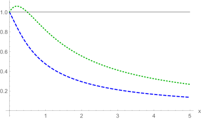
Figure 1: Comparison of the violation of the Mermin inequality in the state $|\xi(k,k^{\pi})\rangle$ (blue, dashed line) and in the state $|\psi(k,k^{\pi})\rangle$ (green, dotted line). The configuration of particles momenta and measurements directions is the following: $\textbf{n}=(0,0,1)$, $\textbf{w}=(\cos\phi_{w}\sin\theta_{w},\sin\phi_{w}\sin\theta_{w},\cos\theta_{w})$, $\textbf{w}\in\{\textbf{a},\textbf{b},\textbf{c}\}$ and $\theta_{a}=1.593$, $\phi_{a}=3.236$, $\theta_{b}=1.564$, $\phi_{b}=1.150$, $\theta_{c}=1.514$, $\phi_{c}=5.322$.

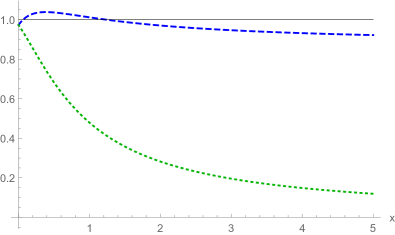
Figure 2: Comparison of the violation of the Mermin inequality in the state $|\xi(k,k^{\pi})\rangle$ (blue, dashed line) and in the state $|\psi(k,k^{\pi})\rangle$ (green, dotted line). The configuration of particles momenta and measurements directions is the following: $\textbf{n}=(0,0,1)$, $\textbf{w}=(\cos\phi_{w}\sin\theta_{w},\sin\phi_{w}\sin\theta_{w},\cos\theta_{w})$, $\textbf{w}\in\{\textbf{a},\textbf{b},\textbf{c}\}$ and $\theta_{a}=1.891$, $\phi_{a}=3.820$, $\theta_{b}=2.589$, $\phi_{b}=0.653$, $\theta_{c}=0.220$, $\phi_{c}=0.716$.

CGLMP inequality.

The CGLMP inequality is an optimal inequality for detecting quantum nonlocality in a system of two qudits. For two qubits it reduces to the CHSH inequality. We consider here spin one bosons therefore we present the CGLMP inequality for two qutrits. We assume that Alice can perform two possible measurements $A_{1}$ or $A_{2}$, and Bob can perform measurements $B_{1}$ or $B_{2}$. Each of these measurements can have three outcomes: 0,1,2. Denoting by $P(A_{i}=B_{j}+k)$ the probability that the outcomes $A_{i}$ and $B_{j}$ differ by $k$ modulo 3, i.e., $P(A_{i}=B_{j}+k)=\sum_{l=0}^{l=2}P(A_{i}=l,B_{j}=l+k\mod 3)$, and defining

$$\mathcal{I}_{3}=\big{[}P(A_{1}=B_{1})+P(B_{1}=A_{2}+1)\\ +P(A_{2}=B_{2})+P(B_{2}=A_{1})\big{]}\\ -\big{[}P(A_{1}=B_{1}-1)+P(B_{1}=A_{2})\\ +P(A_{2}=B_{2}-1)+P(B_{2}=A_{1}-1)\big{]},$$ (49)

the CGLMP inequality can be written in the form

$$\mathcal{I}_{3}\leq 2.$$ (50)

Identifying spin projection values $-1,0,1$ with outcomes $0,1,2$ in the following way

$$-1\leftrightarrow 0,\quad 0\leftrightarrow 1,\quad 1\leftrightarrow 2,$$ (51)

and measurements $A_{1}$, $B_{1}$, $A_{2}$, $B_{2}$ with spin projections on a, b, c, d, respectively, the $\mathcal{I}_{3}$ takes the form

$$\mathcal{I}_{3}=C(\textbf{a},\textbf{b})+C(\textbf{c},\textbf{d})+C(\textbf{a},\textbf{d})-C(\textbf{c},\textbf{b})\\ +P_{+-}(\textbf{a},\textbf{b})+P_{+-}(\textbf{c},\textbf{d})+P_{-+}(\textbf{a},\textbf{d})-P_{+-}(\textbf{c},\textbf{b})\\ +P_{00}(\textbf{a},\textbf{b})+P_{00}(\textbf{c},\textbf{d})+P_{00}(\textbf{a},\textbf{d})-P_{00}(\textbf{c},\textbf{b})\\ -\big{[}P_{0-}(\textbf{a},\textbf{b})+P_{0-}(\textbf{c},\textbf{d})+P_{-0}(\textbf{a},\textbf{d})-P_{0-}(\textbf{c},\textbf{b})\\ +P_{+0}(\textbf{a},\textbf{b})+P_{+0}(\textbf{c},\textbf{d})+P_{0+}(\textbf{a},\textbf{d})-P_{+0}(\textbf{c},\textbf{b})\big{]}.$$ (52)

The probabilities and correlation functions in Eq. (52) are given in Eqs. (33) and (35). We have found that bosons can violate the CGLMP inequality either in the state $|\psi(k,k^{\pi})\rangle$ or in the state $|\xi(k,k^{\pi})\rangle$. In Figs. 3, 4, 5 we have compared the violation of the CGLMP inequality for the states $|\psi(k,k^{\pi})\rangle$ and $|\xi(k,k^{\pi})\rangle$ in different configurations. In all these figures the point $x=0$ corresponds to the nonrelativistic case.

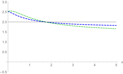
Figure 3: Comparison of the violation of the CGLMP inequality in the state $|\xi(k,k^{\pi})\rangle$ (blue, dashed line) and in the state $|\psi(k,k^{\pi})\rangle$ (green, dotted line). The configuration of particles momenta and measurements directions is the following: $\textbf{n}=(0,0,1)$, $\textbf{w}=(\cos\phi_{w}\sin\theta_{w},\sin\phi_{w}\sin\theta_{w},\cos\theta_{w})$, $\textbf{w}\in\{\textbf{a},\textbf{b},\textbf{c},\textbf{d}\}$ and $\theta_{a}=2.667$, $\phi_{a}=4.109$, $\theta_{b}=0.924$, $\phi_{b}=0.974$, $\theta_{c}=2.699$, $\phi_{c}=1.005$, $\theta_{d}=0$, $\phi_{d}=0$.

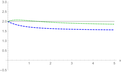
Figure 4: Comparison of the violation of the CGLMP inequality in the state $|\xi(k,k^{\pi})\rangle$ (blue, dashed line) and in the state $|\psi(k,k^{\pi})\rangle$ (green, dotted line). The configuration of particles momenta and measurements directions is the following: $\textbf{n}=(0,0,1)$, $\textbf{w}=(\cos\phi_{w}\sin\theta_{w},\sin\phi_{w}\sin\theta_{w},\cos\theta_{w})$, $\textbf{w}\in\{\textbf{a},\textbf{b},\textbf{c},\textbf{d}\}$ and $\theta_{a}=3.141$, $\phi_{a}=0$, $\theta_{b}=0$, $\phi_{b}=0$, $\theta_{c}=0.836$, $\phi_{c}=5.044$, $\theta_{d}=2.754$, $\phi_{d}=1.897$.

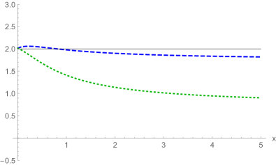
Figure 5: Comparison of the violation of the CGLMP inequality in the state $|\xi(k,k^{\pi})\rangle$ (blue, dashed line) and in the state $|\psi(k,k^{\pi})\rangle$ (green, dotted line). The configuration of particles momenta and measurements directions is the following: $\textbf{n}=(0,0,1)$, $\textbf{w}=(\cos\phi_{w}\sin\theta_{w},\sin\phi_{w}\sin\theta_{w},\cos\theta_{w})$, $\textbf{w}\in\{\textbf{a},\textbf{b},\textbf{c},\textbf{d}\}$ and $\theta_{a}=2.532$, $\phi_{a}=3.141$, $\theta_{b}=1.213$, $\phi_{b}=0$, $\theta_{c}=2.378$, $\phi_{c}=1.363$, $\theta_{d}=0$, $\phi_{d}=0$.

6 Conclusions

The recent paper [32] suggested that it might be possible to experimentally test the violation of Bell inequalities with a pair of $W^{+}W^{-}$ bosons. Motivated by this paper and by our previous theoretical works [21, 37] we have discussed the violation of the Mermin and CGLMP inequalities in a system of two relativistic vector bosons in a scalar state. We have derived formulas for probabilities in the EPR-type experiment in the general scalar state (2), assuming that Alice and Bob measure spin projections on given directions. These probabilities depend on spin projection direction and bosons momenta. We have considered in detail the situation when Alice and Bob are at rest in the center of mass frame of the boson pair. In this case we have explicitly calculated probabilities in two states of particular interest: the simplest nonseparable state $|\psi\rangle$ (6) and the state which in the massless limit converges to the scalar two-photon state $|\xi\rangle$ (8). We have shown that both the Mermin and CGLMP inequalities can be violated in both states $|\psi\rangle$ and $|\xi\rangle$ and that the degree of violation depends on bosons momenta.

Large violations of the CGLMP inequality are predicted even for boson pairs at rest. For small boosts of the vector bosons, both the Mermin, and more particularly the CGLMP inequalities show sufficiently large violations that they might well be measurable in practical experiments. For the CGLMP inequality, our analytical results, here calculated in the narrow-width approximation, and with observers at rest in the centre-of-mass-frame of the boson pair, support the conclusion found using numerical results in simulations of $H\to WW^{*}$ decays in Ref. [32] under different assumptions.

Potential applications of these results extend beyond the case of Higgs boson decays. Other example applications might include relativistic hadronic, nuclear, atomic or molecular systems.

Appendix A Massive representations of the Poincaré group for $s=1$

For self-consistency we recall here basic facts related to massive spin 1 representations of the Poincaré group. For more details see, e.g, [53]. Let $\mathcal{H}$ be the carrier space of the irreducible massive representation of the Poincaré group for $s=1$. $\mathcal{H}$ is spanned by the four-momentum operator eigenvectors $|k,\sigma\rangle$

$$\hat{P}^{\mu}|k,\sigma\rangle=k^{\mu}|k,\sigma\rangle,$$ (53)

$k^{2}=m^{2}$, $m$ is the mass of the particle, and $\sigma$ its spin component along $z$ axis, $\sigma=-1,0,1$. We use the following Lorentz-covariant normalization

$$\langle k,\sigma|k^{\prime},\sigma^{\prime}\rangle=2k^{0}\delta^{3}(\textbf{k}-\textbf{k}^{\prime})\delta_{\sigma\sigma^{\prime}}.$$ (54)

The vectors $|k,\sigma\rangle$ can be generated from the standard vector $|\tilde{k},\sigma\rangle$, where $\tilde{k}=m(1,0,0,0)$ is the four-momentum of the particle in its rest frame. We have $|k,\sigma\rangle=U(L_{k})|\tilde{k},\sigma\rangle$, where Lorentz boost $L_{k}$ is defined by relations $k=L_{k}\tilde{k}$, $L_{\tilde{k}}={\mathbb{I}}$.

By means of Wigner procedure we get

$$U(\Lambda)|k,\sigma\rangle=\mathcal{D}_{\lambda\sigma}(R(\Lambda,k))|\Lambda k,\lambda\rangle,$$ (55)

where the Wigner rotation $R(\Lambda,k)$ is defined as $R(\Lambda,k)=L_{\Lambda k}^{-1}\Lambda L_{k}$, and for $s=1$ the representation $\mathcal{D}(R)$ is unitary equivalent to $R$ by

$$\mathcal{D}(R)=VRV^{{\dagger}},\qquad V^{\dagger}V={\mathbb{I}},$$ (56)

and the explicit form of the matrix $V$ is the following:

$$V=\frac{1}{\sqrt{2}}\begin{pmatrix}-1&i&0\\ 0&0&\sqrt{2}\\ 1&i&0\\ \end{pmatrix}.$$ (57)

Appendix B Boson field

In order to describe two types of vector bosons, particle and antiparticle (e.g. $W^{+}$ and $W^{-}$), we consider the free field operator $\hat{\phi}^{\mu}(x)$ with the following momentum expansion:

$$\hat{\phi}^{\mu}(x)=(2\pi)^{(-3/2)}\int\tfrac{d^{3}\textbf{k}}{2\omega_{k}}\big{[}e^{ikx}e^{\mu}_{\sigma}(k)a^{\dagger}_{\sigma}(k)\\ +e^{-ikx}e^{*\mu}_{\sigma}(k)b_{\sigma}(k)\big{]},$$ (58)

where $\omega_{k}=\sqrt{\textbf{k}^{2}+m^{2}}$ and $m$ is a mass of a particle (and antiparticle). $a^{\dagger}_{\sigma}(k)$, $a_{\sigma}(k)$ and $b^{\dagger}_{\sigma}(k)$, $b_{\sigma}(k)$ are creation and annihilation operators of a particle and antiparticle, respectively. $a^{\dagger}_{\sigma}(k)$ ($b^{\dagger}_{\sigma}(k)$) creates particle (antiparticle) with four-momentum $k$ and spin component along $x$ axis equal to $\sigma$. They fulfill the standard canonical commutation relations

$$[a_{\sigma}(k),a^{\dagger}_{\sigma^{\prime}}(k^{\prime})]=[b_{\sigma}(k),b^{\dagger}_{\sigma^{\prime}}(k^{\prime})]=2k^{0}\delta(\textbf{k}-\textbf{k}^{\prime})\delta_{\sigma\sigma^{\prime}}$$ (59)

and all the other commutators vanish. The Klein-Gordon equation and Lorentz transversality condition imply

$$k^{2}=m^{2},\quad k_{\mu}e^{\mu}_{\sigma}(k)=0.$$ (60)

The one-particle and one-antiparticle states

$$|k,\lambda\rangle_{a}=a^{\dagger}_{\lambda}(k)|0\rangle,\quad|p,\sigma\rangle_{b}=b^{\dagger}_{\sigma}(p)|0\rangle,$$ (61)

where $|0\rangle$ is a Lorentz-invariant vacuum, $\langle 0|0\rangle=1$, should transform like a basis states of a carrier space of the irreducible, massive representation of the Poincaré group for $s=1$ considered in Appendix A. This condition allows us to determine the explicit form of amplitudes $e^{\mu}_{\sigma}(k)$. The derivation is the same as in [21], therefore we give here only the results:

$$e(k)=[e^{\mu}_{\sigma}(k)]=\begin{pmatrix}\tfrac{\textbf{k}^{T}}{m}\\ {\mathbb{I}}+\tfrac{\textbf{k}\otimes\textbf{k}^{T}}{m(m+k^{0})}\end{pmatrix}V^{T},$$ (62)

where $V$ is given in Eq. (57). Moreover, one can show that $e^{\mu}_{\sigma}(k)$ fulfills the following relations:

$$e^{*}(k)=e(k)VV^{T},$$ (63)

$$e^{*\mu}_{\sigma}(k)e^{\nu}_{\sigma}(k)=-\eta^{\mu\nu}+\tfrac{k^{\mu}k^{\nu}}{m^{2}},$$ (64)

$$e^{*\mu}_{\sigma}(k)e_{\mu\lambda}(k)=-\delta_{\sigma\lambda},$$ (65)

$$e^{\mu}_{\sigma}(k)e_{\mu\lambda}(k)=-(VV^{T})_{\sigma\lambda}.$$ (66)

Appendix C Boson states transforming covariantly under Lorentz transformations

In [21] it was shown that with the help of amplitudes $e^{\mu}_{\sigma}(k)$ one can construct states transforming in the explicitly covariant manner under Lorentz transformations. In our case covariant particle/anti-particle states have the form

$$|(\mu,k)\rangle_{a/b}=e^{\mu}_{\sigma}(k)|k,\sigma\rangle_{a/b},$$ (67)

and under Lorentz transformations transform according to

$$U(\Lambda)|(\mu,k)\rangle_{a/b}=(\Lambda^{-1})^{\mu}_{\nu}|(\nu,\Lambda k)\rangle_{a/b}.$$ (68)

Two-particle state describing boson with four-momentum $k$ and spin projection $\lambda$ and antiboson with four-momentum $p$ and spin projection $\sigma$ has the form

$$|(k,\lambda)_{a};(p,\sigma)_{b}\rangle=a^{\dagger}_{\sigma}(k)b^{\dagger}_{\sigma}(p)|0\rangle,$$ (69)

and consequently a boson–antiboson covariant state reads

$$e^{\mu}_{\lambda}(k)e^{\nu}_{\sigma}(p)|(k,\lambda)_{a};(p,\sigma)_{b}\rangle.$$ (70)

Appendix D Localization inside detectors

Eigenvectors of the Newton–Wigner operator have the following form[26]

$$|\textbf{x},\sigma\rangle=\frac{1}{(2\pi)^{3/2}}\int\frac{d^{3}\textbf{p}}{2p^{0}}\sqrt{2p^{0}}e^{-i\textbf{p}\cdot\textbf{x}}|p,\sigma\rangle,$$ (71)

where $p^{0}=\sqrt{\textbf{p}^{2}+m^{2}}$. The problem of localization of a particle inside a detector during spin measurement in the context of relativistic quantum correlations of a fermion pair was also discussed in [26]. Here we briefly present that paper’s conclusions, adapting them to a system of vector bosons. The central element in such a discussion is the projector on a region $D$ in the coordinate space

$$\hat{\Pi}_{D} =\int_{D}d^{3}\textbf{x}\sum_{\sigma=-1,0,1}|\textbf{x},\sigma\rangle\langle\textbf{x},\sigma|$$ (72)

$$=\iint\limits_{{{\mathbb{R}}^{3}\times{\mathbb{R}}^{3}}}\frac{d^{3}\textbf{p}}{\sqrt{2p^{0}}}\frac{d^{3}\textbf{p}^{\prime}}{\sqrt{2{p^{\prime}}^{0}}}\Delta_{D}(\textbf{p}^{\prime}-\textbf{p})\sum_{\sigma}|p^{\prime},\sigma\rangle\langle p,\sigma|,$$ (73)

where $|\textbf{x},\sigma\rangle$ is defined in (71) and

$$\Delta_{D}(\textbf{p}^{\prime}-\textbf{p}) =\frac{1}{(2\pi)^{3}}\int_{D}d^{3}\textbf{x}e^{-i(\textbf{p}^{\prime}-\textbf{p})\cdot\textbf{x}}$$ (74)

$$=\frac{1}{(2\pi\hbar)^{3}}\int_{D}d^{3}\textbf{x}e^{-i\frac{(\textbf{p}^{\prime}-\textbf{p})\cdot\textbf{x}}{mc\lambda}}.$$ (75)

To facilitate further discussion, in the second line we have explicitly expressed $\Delta_{D}$ in the standard units, $c$ is the velocity of light and $\lambda=\frac{\lambda_{C}}{2\pi}=\frac{\hbar}{mc}$ is the particle Compton wavelength divided by $2\pi$. To evaluate quantitatively the influence of localization let us choose $D$ as the cube located in the center of the coordinate frame with edges of the length $l$ parallel to coordinate axis. In this case $\Delta_{\textsf{Cube}}$ can be calculated and we obtain

$$\Delta_{\textsf{Cube}}(\textbf{p}^{\prime}-\textbf{p})=\Big{(}\frac{\lambda}{\hbar}\Big{)}^{3}\prod_{j=1}^{3}\Big{[}\frac{1}{\pi}\frac{l}{2\lambda}\mathrm{sinc}\,\Big{(}\frac{p_{j}^{\prime}-p_{j}}{mc}\frac{l}{2\lambda}\Big{)}\Big{]}.$$ (76)

Using the formula

$$\lim\limits_{\tau\to\infty}\frac{\tau}{\pi}\mathrm{sinc}\,(\tau x)=\delta(x)$$ (77)

we observe that for $l\to\infty$: $\Delta_{\textsf{Cube}}(\textbf{p}^{\prime}-\textbf{p})\to\delta^{3}(\textbf{p}^{\prime}-\textbf{p})$ and consequently

$$\hat{\Pi}_{D}\to\hat{\Pi}_{{\mathbb{R}}^{3}}=I.$$ (78)

Therefore, there is no problem with localization of a quantum particle provided that its Compton wavelength is sufficiently small in comparison with a detecting element size $l$, i.e., when the condition $\lambda\ll l$ holds.

For muons and electrons at rest the corresponding Compton wavelengths take the following approximate values: $\lambda_{\mu}=1.87\times 10^{-15}$ m and $\lambda_{e}=3.86\times 10^{-13}$ m. Consequently, assuming a realistic size of particle detector pixels $l=10^{-6}$ m, the scaling factors $\tau=l/(2\lambda)$ take the values $\tau_{\mu}=0.27\times 10^{9}$ and $\tau_{e}=0.13\times 10^{7}$, respectively. Moreover, for relativistic particles we should use $m=\gamma m_{\textsf{rest}}$, where $\gamma$ is the particle Lorentz factor, so $\lambda=\gamma^{-1}\lambda_{\textsf{rest}}$ and in effect the Compton wavelength decreases so the scaling factor increases. Thus, for real, massive particles $\Delta_{\textsf{Cube}}(\textbf{p}^{\prime}-\textbf{p})$ is very close to $\delta^{3}(\textbf{p}^{\prime}-\textbf{p})$ and, indeed, there is no problem with localization of a particle inside the detector in situation in which it is directly detected.

References

• [1] A. Einstein, B. Podolsky, and N. Rosen. “Can quantum-mechanical description of physical reality be considered complete?”. Phys. Rev. 47, 777–780 (1935).
• [2] John S. Bell. “On the Einstein Podolsky Rosen paradox”. Physics Physique Fizika 1, 195–200 (1964).
• [3] Stuart J. Freedman and John F. Clauser. “Experimental test of local hidden-variable theories”. Phys. Rev. Lett. 28, 938–941 (1972).
• [4] Alain Aspect, Jean Dalibard, and Gérard Roger. “Experimental test of Bell’s inequalities using time-varying analyzers”. Phys. Rev. Lett. 49, 1804–1807 (1982).
• [5] M. A. Rowe, D. Kielpinski, V. Meyer, C. A. Sackett, W. M. Itano, C. Monroe, and D. J. Wineland. “Experimental violation of a Bell’s inequality with efficient detection”. Nature 409, 791–794 (2001).
• [6] Markus Ansmann et al. “Violation of Bell’s inequality in Josephson phase qubits”. Nature 461, 504–506 (2009).
• [7] Wolfgang Pfaff, Tim H. Taminiau, Lucio Robledo, Hannes Bernien, Matthew Markham, Daniel J. Twitchen, and Ronald Hanson. “Demonstration of entanglement-by-measurement of solid-state qubits”. Nature Physics 9, 29–33 (2013).
• [8] B. Hensen et al. “Loophole-free Bell inequality violation using electron spins separated by 1.3 kilometres”. Nature 526, 682–686 (2015).
• [9] Marissa Giustina et al. “Significant-loophole-free test of Bell’s theorem with entangled photons”. Phys. Rev. Lett. 115, 250401 (2015).
• [10] Lynden K. Shalm et al. “Strong loophole-free test of local realism”. Phys. Rev. Lett. 115, 250402 (2015).
• [11] Alipasha Vaziri, Gregor Weihs, and Anton Zeilinger. “Experimental two-photon, three-dimensional entanglement for quantum communication”. Phys. Rev. Lett. 89, 240401 (2002).
• [12] Marek Czachor. “Einstein-Podolsky-Rosen-Bohm experiment with relativistic massive particles”. Phys. Rev. A 55, 72–77 (1997).
• [13] Paul M. Alsing and Gerard J. Milburn. “On entanglement and Lorentz transfotmations”. Quantum Info. Comput. 2, 487 (2002).
• [14] Robert M. Gingrich and Christoph Adami. “Quantum entanglement of moving bodies”. Phys. Rev. Lett. 89, 270402 (2002).
• [15] Asher Peres, Petra F. Scudo, and Daniel R. Terno. “Quantum entropy and special relativity”. Phys. Rev. Lett. 88, 230402 (2002).
• [16] Doyeol Ahn, Hyuk-jae Lee, Young Hoon Moon, and Sung Woo Hwang. “Relativistic entanglement and Bell’s inequality”. Phys. Rev. A 67, 012103 (2003).
• [17] Hui Li and Jiangfeng Du. “Relativistic invariant quantum entanglement between the spins of moving bodies”. Phys. Rev. A 68, 022108 (2003).
• [18] H. Terashima and M. Ueda. “Relativistic Einstein–Podolsky–Rosen correlation and Bell’s inequality”. Int. J. Quant. Inf. 1, 93–114 (2003).
• [19] Paweł Caban and Jakub Rembieliński. “Lorentz-covariant reduced spin density matrix and Einstein–Podolsky–Rosen–Bohm correlations”. Phys. Rev. A 72, 012103 (2005).
• [20] Paweł Caban and Jakub Rembieliński. “Einstein-Podolsky-Rosen correlations of Dirac particles: Quantum field theory approach”. Phys. Rev. A 74, 042103 (2006).
• [21] Paweł Caban, Jakub Rembieliński, and Marta Włodarczyk. “Einstein-Podolsky-Rosen correlations of vector bosons”. Phys. Rev. A 77, 012103 (2008).
• [22] Nicolai Friis, Reinhold A. Bertlmann, Marcus Huber, and Beatrix C. Hiesmayr. “Relativistic entanglement of two massive particles”. Phys. Rev. A 81, 042114 (2010).
• [23] Paul M Alsing and Ivette Fuentes. “Observer-dependent entanglement”. Classical and Quantum Gravity 29, 224001 (2012).
• [24] Pablo L. Saldanha and Vlatko Vedral. “Spin quantum correlations of relativistic particles”. Phys. Rev. A 85, 062101 (2012).
• [25] E. R. F. Taillebois and A. T. Avelar. “Spin-reduced density matrices for relativistic particles”. Phys. Rev. A 88, 060302 (2013).
• [26] Paweł Caban, Jakub Rembieliński, Patrycja Rybka, Kordian A. Smoliński, and Piotr Witas. “Relativistic Einstein-Podolsky-Rosen correlations and localization”. Phys. Rev. A 89, 032107 (2014).
• [27] Veiko Palge and Jacob Dunningham. “Behavior of Werner states under relativistic boosts”. Ann. Phys. 363, 275–304 (2015).
• [28] Victor A. S. V. Bittencourt, Alex E. Bernardini, and Massimo Blasone. “Global Dirac bispinor entanglement under Lorentz boosts”. Phys. Rev. A 97, 032106 (2018).
• [29] Lucas F. Streiter, Flaminia Giacomini, and Časlav Brukner. “Relativistic Bell test within quantum reference frames”. Phys. Rev. Lett. 126, 230403 (2021).
• [30] Matthias Ondra and Beatrix C. Hiesmayr. “Single particle entanglement in the mid- and ultra-relativistic regime”. J. Phys. A: Math. Theor. 54, 435301 (2021).
• [31] H. Bacry. “Localizability and space in quantum physics”. Lecture Notes in Physics Vol. 308. Springer–Verlag. Berlin, Heidelberg (1988).
• [32] Alan J. Barr. “Testing Bell inequalities in Higgs boson decays”. Phys. Lett. B 825, 136866 (2022).
• [33] J. A. Aguilar-Saavedra, A. Bernal, J. A. Casas, and J. M. Moreno. “Testing entanglement and Bell inequalities in ${H}\rightarrow{ZZ}$”. Phys. Rev. D 107, 016012 (2023).
• [34] Rachel Ashby-Pickering, Alan J. Barr, and Agnieszka Wierzchucka. “Quantum state tomography, entanglement detection and Bell violation prospects in weak decays of massive particles”. J. High Energ. Phys. 2023, 20 (2023).
• [35] J. A. Aguilar-Saavedra. “Laboratory-frame tests of quantum entanglement in $H\rightarrow WW$”. Phys. Rev. D 107, 076016 (2023).
• [36] M. Fabbrichesi, R. Floreanini, E. Gabrielli, and L. Marzola. “Bell inequalities and quantum entanglement in weak gauge bosons production at the LHC and future colliders” (2023). arXiv:2302.00683.
• [37] Paweł Caban. “Helicity correlations of vector bosons”. Phys. Rev. A 77, 062101 (2008).
• [38] T. D. Newton and E. P. Wigner. “Localized states for elementary systems”. Rev. Mod. Phys. 21, 400–406 (1949).
• [39] N. N. Bogolubov, A. A. Logunov, and I. T. Todorov. “Introduction to axiomatic quantum field theory”. W. A. Benjamin. Reading, Mass. (1975).
• [40] Paweł Caban, Jakub Rembieliński, and Marta Włodarczyk. “A spin observable for a Dirac particle”. Ann. of Phys. 330, 263–272 (2013).
• [41] Paweł Caban, Jakub Rembieliński, and Marta Włodarczyk. “Strange behavior of the relativistic Einstein-Podolsky-Rosen correlations”. Phys. Rev. A 79, 014102 (2009).
• [42] Daniel R. Terno. “Two roles of relativistic spin operators”. Phys. Rev. A 67, 014102 (2003).
• [43] Pablo L Saldanha and Vlatko Vedral. “Physical interpretation of the Wigner rotations and its implications for relativistic quantum information”. New J. Phys. 14, 023041 (2012).
• [44] Heiko Bauke, Sven Ahrens, Christoph H. Keitel, and Rainer Grobe. “What is the relativistic spin operator?”. New J. Phys. 16, 043012 (2014).
• [45] Lucas C. Céleri, Vasilis Kiosses, and Daniel R. Terno. “Spin and localization of relativistic fermions and uncertainty relations”. Phys. Rev. A 94, 062115 (2016).
• [46] Liping Zou, Pengming Zhang, and Alexander J. Silenko. “Position and spin in relativistic quantum mechanics”. Phys. Rev. A 101, 032117 (2020).
• [47] E.R.F. Taillebois and A.T. Avelar. “Relativistic spin operator must be intrinsic”. Phys. Lett. A 392, 127166 (2021).
• [48] Heon Lee. “Relativistic massive particle with spin-1/2: A vector bundle point of view”. J. Math. Phys. 63, 012201 (2022).
• [49] Leslie E Ballentine. “Quantum mechanics: A modern development”. World Scientific.  (2014). 2nd edition.
• [50] John F. Clauser, Michael A. Horne, Abner Shimony, and Richard A. Holt. “Proposed experiment to test local hidden-variable theories”. Phys. Rev. Lett. 23, 880–884 (1969).
• [51] N. D. Mermin. “Quantum mechanics vs local realism near the classical limit: A Bell inequality for spin $s$”. Phys. Rev. D 22, 356–361 (1980).
• [52] Daniel Collins, Nicolas Gisin, Noah Linden, Serge Massar, and Sandu Popescu. “Bell inequalities for arbitrarily high-dimensional systems”. Phys. Rev. Lett. 88, 040404 (2002).
• [53] A Barut and R Raczka. “Theory of group representations and applications”. World Scientific.  (1986).