Differentially Private Learning with Margin Guarantees

Abstract

We present a series of new differentially private (DP) algorithms with dimension-independent margin guarantees. For the family of linear hypotheses, we give a pure DP learning algorithm that benefits from relative deviation margin guarantees, as well as an efficient DP learning algorithm with margin guarantees. We also present a new efficient DP learning algorithm with margin guarantees for kernel-based hypotheses with shift-invariant kernels, such as Gaussian kernels, and point out how our results can be extended to other kernels using oblivious sketching techniques. We further give a pure DP learning algorithm for a family of feed-forward neural networks for which we prove margin guarantees that are independent of the input dimension. Additionally, we describe a general label DP learning algorithm, which benefits from relative deviation margin bounds and is applicable to a broad family of hypothesis sets, including that of neural networks. Finally, we show how our DP learning algorithms can be augmented in a general way to include model selection, to select the best confidence margin parameter.

1 Introduction

Preserving privacy is a crucial objective for machine learning algorithms. A widely adopted criterion in statistical data privacy is the notion of differential privacy (DP) [DMNS06, Dwo06, DR14], which ensures that the information gained by an adversary is roughly invariant to the presence or absence of an individual in a dataset. Despite the remarkable theoretical and algorithmic progress in differential privacy over the last decade or more, however, its application to learning still faces several obstacles. A recent series of publications have shown that differentially private PAC learning of infinite hypothesis sets is not possible, even for common hypothesis sets such as that of linear functions. In fact, this is the case for any hypothesis set containing threshold functions [BNSV15, ALMM19]. These results imply serious limitations for private agnostic learnability.

Another rich body of literature has studied differentially private empirical risk minimization (DP-ERM) and differentially private stochastic convex optimization (DP-SCO) (e.g., [CMS11, JT14, BST14, BFTT19, FKT20, SSTT21, BGN21, AFKT21, BGM21]). When the underlying optimization problem is constrained (constrained setting), tight upper and lower bounds have been derived for the excess empirical risk of DP-ERM [BST14] and for the excess population risk for DP-SCO [BFTT19, FKT20]. These results show that learning guarantees necessarily admit a dependency on the dimension $d$ of the form $\sqrt{d}/m$, where $m$ is the sample size. This dependency is persistent, even in the special case of generalized linear losses (GLLs) [BST14], which limits the benefit of such guarantees, since learning algorithms typically deal with high-dimensional spaces.

When the underlying optimization problem is unconstrained (unconstrained setting) and the loss is a generalized linear loss, the bounds given by [JT14], [SSTT21] and [BGM21] are dimension-independent but they admit a dependency on $\|w^{\ast}\|^{2}$, where $w^{\ast}$ is the unconstrained minimizer of the expected loss (population risk), or $\|\widehat{w}\|^{2}$, where $\widehat{w}$ is the unconstrained minimizer of the empirical loss. Since the problem is unconstrained, the norm of these vectors can be very large, even for classification problems for which the minimizer of the zero-one loss admits a relatively small norm. Thus, in both the constrained and unconstrained settings, the learning guarantees derived from DP-ERM and DP-SCO are weak for hypothesis sets commonly used in machine learning.

The results just mentioned raise some fundamental questions about private learning: is differentially private learning with favorable (dimension-independent) guarantees possible for standard hypothesis sets? Must one resort to distribution-dependent bounds instead? In view of the negative PAC-learning results and other learning bounds mentioned earlier, we will seek instead optimistic margin-based learning bounds.

In the context of classification, learning bounds for linear hypotheses based on the dimension or, more generally, based on the VC-dimension of the hypothesis set are known to be too pessimistic since they deal with the worst case. Instead, margin bounds have been shown to be the most informative and useful guarantees [KP02, SFBL97]. This motivates our study of differentially private learning algorithms with margin-based guarantees. Note that our confidence-margin analysis and guarantees do not require the hard-margin separability assumptions adopted in [BDMN05, LNUZ20], which is a strong assumption that typically does not hold in practice. Another existing study that deals with somewhat related questions is that of [CHS14]. But, the paper deals with a specific class of maximization problems and adopts a non-standard definition of margin. Another related line of work is that of [RBHT09] and [CMS11] on DP Kernel classifiers, which we discuss in detail in Section 1.1.

Main contributions. We present a series of new differentially private (DP) algorithms with dimension-independent margin guarantees. In Section 3, we study the family of linear hypotheses. We first give a pure DP learning algorithm with relative deviation margin guarantees that is computationally inefficient. Next, we present an efficient DP learning algorithm with margin guarantees. In Section 4, we consider kernel-based hypothesis sets. We present a new efficient DP learning algorithm with margin guarantees for such hypothesis sets, assuming that the positive definite kernel used is shift-invariant, as with the most commonly used Gaussian kernels. We further briefly discuss how recent kernels approximation results using oblivious sketching can be used to extend our results to other kernel functions, including polynomial kernels and many other kernels that can be approximated using polynomial kernels, as well and the neural tangent kernel (NTK) or arc-cosine kernels. In Section 5, we initiate the study of DP learning of neural networks with margin guarantees. We design a pure DP learning algorithm for a family of feed-forward neural networks for which we prove margin guarantees that are independent of input dimension. In Section 6, we further present a label privacy learning algorithm, which we show benefits from relative deviation margin bounds. The algorithm and its guarantee are applicable to a broad family of hypothesis sets, including that of neural networks. In Appendix F, we show how our DP learning algorithms can be augmented in a general way to include model selection, to select the best confidence margin parameter.

Let us emphasize some key novelty of our work: (i) we give algorithms and more favorable learning guarantees than previous work on unconstrained GLLs; (ii) our guarantees and analyses are expressed in terms of the confidence-margin, in contrast with the geometric margin, which relies on a strong separability assumption; (iii) we give a more efficient algorithm for linear classification based on a faster construction for the JL-transform and faster DP-ERM algorithm; (iv) we present new private learning bounds for DP kernel classifiers that are nearly the same as the standard non-private bounds, without resorting to the strong assumptions adopted in prior work; (v) we initiate the study of DP learning of neural nets with margin guarantees and derive the first margin bound for this problem that has no dependence on the input dimension and better dependence on the network parameters than the bounds attained via uniform convergence.

We also wish to highlight the novelty of our analysis: (i) while the general structure of our algorithms for linear classifiers is superficially similar to that of [LNUZ20], our results require a new analysis that takes into account the scale-sensitive nature of the margin loss and the $\rho$-hinge loss; (ii) our solutions include new algorithmic ideas and analyses for DP kernel classifiers, such as the use of JL-transform and a new analysis that uses regularized ERM as a reference; (iii) our margin bound for DP neural nets entails a new analysis of embedding-based “network compression” technique. It is also important to point out that, even though we use the $\rho$-hinge loss in our efficient constructions for linear and kernel classifiers, our results can be easily extended to other convex surrogates for the zero-one loss, such as the logistic loss.

1.1 Related work

In this section, we discuss in more detail other previous studies that are the most directly related to the work we present.

Prior work on unconstrained GLLs. [JT14] and [SSTT21] showed that it is possible to derive dimension-independent risk bounds for DP-ERM and DP-SCO in the context of linear prediction, when the parameter space is unconstrained and the loss function is convex and Lipschitz (GLL). However, their bounds scale with $\|w^{\ast}\|$, the norm of the optimal unconstrained minimizer of the expected loss of a surrogate loss such as the hinge loss. Also, using their techniques for unconstrained DP-ERM for GLLs together with uniform convergence would yield generalization error bounds that scale with the norm of the unconstrained empirical risk minimizer $\widehat{w}$.

The first issue with this line of work is that the norms of such unconstrained solutions can be very large, thereby resulting in uninformative bounds. In fact, one can construct simple, low-dimensional examples, where $\|w^{\ast}\|=\Omega(m)$ while there is a predictor $w$ with $\|w\|=O(1)$ that attains the same expected zero-one error, see Figure 1. A detailed analysis of that example in presented in Appendix H. Moreover, these studies assume prior knowledge of $\|w^{\ast}\|$, which is not a realistic assumption. Readily applying the techniques of these studies without assuming that prior knowledge results in an explicit dependence on $(1+\|w^{\ast}\|^{2})$, which is even less favorable. Furthermore, estimating this norm privately in the unconstrained setting requires a non-trivial construction and argument. Perhaps more importantly, the paradigm adopted in this line of work is to first devise an algorithm and next derive bounds for its excess risk. In contrast, we start from strong generalization error bounds, which we use to guide the design of our algorithm.

Figure 1: Simple example in dimension one for which the minimizer of the expected hinge loss $\operatorname*{\mathbb{E}}[\ell^{\mathsf{\,hinge}}(w)]$ is $w^{*}=\frac{1}{\gamma}$ and thus $\|w^{*}\|=\frac{1}{\gamma}\gg 1$ for $\gamma\ll 1$. Here, any other $w>0$, in particular with a small norm, achieves the same zero-one loss as $w^{*}$.

Prior work on DP learning of hard-margin halfspaces. [BDMN05] and [LNUZ20] studied DP learning of linear classifiers in the separable setting, that is with a hard- or geometric margin. [BDMN05] gave a construction based on a private version of the Perceptron algorithm, which results in a dimension-independent bound on the expected error. This result was later improved by [LNUZ20] who gave new constructions with dimension-independent guarantees based on embeddings, namely, the Johnson-Lindenstrauss (JL) transform. Note that the hard-margin separability is a strong assumption that typically does not hold in practice. Moreover, the construction suggested by the authors requires knowledge of the margin for their guarantees to be valid. In contrast, our work considers the more general notion of confidence margin, which does not require the existence of a geometric margin and applies to realistic scenarios with non-separable data. Moreover, the confidence-margin parameter, $\rho$, in our algorithms is tunable and can be optimized (which we do in Appendix F). Importantly, our algorithms still yields meaningful learning guarantees even if this parameter is not optimized. Our algorithms for linear classifiers also makes use of an embedding as pre-processing step. However despite a structure similar on the surface to that of [LNUZ20], our algorithm requires a new analysis together as well as a precise setting of the parameters. This includes a careful analysis to deal with the scale-sensitive nature of our bounds, due to the absence of a hard-margin. This is evident in the setting of the embedding parameters in our efficient algorithm based on the hinge loss, which is different from that in [LNUZ20]. In particular, in our setting, we choose the embedding dimension to be approximately $m$ to control the impact of the embedding approximation error on the empirical hinge loss when a hard margin is absent or unknown.

Prior work on DP Kernel classifiers. [RBHT09] were the first to provide differentially private constructions for SVMs in both the finite-dimensional feature space and kernel settings. However, their constructions are suboptimal and the resulting bounds suffer from a polynomial dependence on the dimension of the feature space. In particular, they consider SVM learning with a shift-invariant kernel. Their algorithm in this case is based on defining a finite-dimensional approximation of the kernel using the technique of [RR07], which reduces the problem to a finite-dimensional SVM learning problem. Their private solution is based on perturbing the non-private finite-dimensional predictor. In addition to the polynomial dependence on the input dimension, their error bound in this case is sub-optimal in its dependence on the sample size $m$ and admits an explicit dependence on the on the $L_{1}$-norm of the dual variables of the SVM [RBHT09, Theorem 14]. In general, this norm can be as large as $\sqrt{m}$ and, in such cases, their error bound becomes vacuous.

[CMS11] gave a similar construction for shift-invariant kernels. However, their error guarantees are based on the kernel approximation results of [RR08] and hence entail a relatively strong assumption on the Fourier coefficients of the kernel predictors. In particular, they assume that the Fourier transform of the optimal predictor decays at a faster rate than the kernel density. We note that the standard assumption of bounded Reproducing Kernel Hilbert Space (RKHS) norm does not imply such a condition.

[JT13] gave algorithms for DP predictions with kernels. They considered scenarios where the goal is to privately generate predictions (labels) on a small test set that admits no privacy constraints. In such scenarios, their algorithms do not output a classifier. The solution is interactive and limited to answering a small number of classification queries, within some privacy budget. [JT13] also considered the non-interactive case, however, their construction in this setting is computationally inefficient and the resulting error guarantees are dimension-dependent.

In this work, we give a new private construction for shift-invariant kernel classifiers and derive an error bound that nearly matches (up to a factor of $\widetilde{O}(1/\varepsilon)$) the optimal non-private bound under standard problem setup (kernel predictors with bounded RKHS norm). Our algorithm also runs in polynomial time. These improvements over prior work hold thanks to the use of our private algorithm for linear classifiers after approximating the kernel together with a tighter error analysis that does not require any non-standard assumptions. We also show how to achieve similar results for polynomial kernels (which are not necessarily shift-invariant) by using an embedding such as the JL-transform as well as other, more efficient techniques, such as oblivious sketches.

We start with the introduction of some basic definitions and concepts needed for our discussion.

2 Preliminaries

We consider an input space $\mathcal{X}$, a binary output space $\mathcal{Y}=\{-1,+1\}$ and a hypothesis set ${\mathscr{H}}$ of functions mapping from $\mathcal{X}$ to $\mathbb{R}$. We denote by $\mathscr{D}$ a distribution over $\mathcal{Z}=\mathcal{X}\times\mathcal{Y}$ and denote by $R_{\mathscr{D}}(h)$ the generalization error and by $\widehat{R}_{S}(h)$ the empirical error of a hypothesis $h\in{\mathscr{H}}$:

$$R_{\mathscr{D}}(h)=\operatorname*{\mathbb{E}}_{z=(x,y)\sim\mathscr{D}}[1_{yh(x)\leq 0}]\qquad\widehat{R}_{S}(h)=\operatorname*{\mathbb{E}}_{z=(x,y)\sim S}[1_{yh(x)\leq 0}],$$

where we write $z\sim S$ to indicate that $z$ is randomly drawn from the empirical distribution defined by $S$. Given $\rho\geq 0$, we similarly define the $\rho$-margin loss and empirical $\rho$-margin loss of $h\in{\mathscr{H}}$:

$$R^{\rho}_{\mathscr{D}}(h)=\operatorname*{\mathbb{E}}_{z=(x,y)\sim\mathscr{D}}[1_{yh(x)\leq\rho}]\qquad\widehat{R}^{\rho}_{S}(h)=\operatorname*{\mathbb{E}}_{z=(x,y)\sim S}[1_{yh(x)\leq\rho}].$$

The $\rho$-margin loss is not convex. Hence, we also consider $\rho$-hinge loss to provide computationally-efficient algorithms. For any $\rho>0$, define $\rho$-hinge loss as $\ell^{\rho}(u)\triangleq\max\left(1-u/\rho,\,0\right),~{}u\in\mathbb{R}$. Similar to the above definitions, given $\rho>0$, for a sample $S$, we define the $\rho$-hinge loss and empirical $\rho$-hinge loss as

$$L^{\rho}_{\mathscr{D}}(w)=\operatorname*{\mathbb{E}}_{z=(x,y)\sim\mathscr{D}}[\ell^{\rho}\left(y_{i}\,\langle w,x_{i}\rangle\right)]\qquad\widehat{L}^{\rho}_{S}(w)=\operatorname*{\mathbb{E}}_{z=(x,y)\sim S}[\ell^{\rho}\left(y_{i}\,\langle w,x_{i}\rangle\right)].$$

In the context of learning, differential privacy is defined as follows.

Definition 2.1 (Differential privacy).

Let $\varepsilon,\delta\geq 0$. Let $\mathcal{A}\colon(\mathcal{X}\times\mathcal{Y})^{m}\to{\mathscr{H}}$ be a randomized algorithm. We say that $\mathcal{A}$ is $(\varepsilon,\delta)$-DP if for any measurable subset $O\subset{\mathscr{H}}$ and all $S,S^{\prime}\in(\mathcal{X}\times\mathcal{Y})^{m}$ that differ in one sample, the following inequality holds:

$$\operatorname*{\mathbb{P}}(\mathcal{A}(S)\in O)\leq e^{\varepsilon}\operatorname*{\mathbb{P}}(\mathcal{A}(S^{\prime})\in O)+\delta.$$ (1)

If $\delta=0$, we refer to this guarantee as pure differential privacy.

3 Private Algorithms for Linear Classification with Margin Guarantees

In this section, we present two private learning algorithms for linear classification with margin guarantees: first, a computationally inefficient pure DP algorithm, which we show benefits from relative deviation margin bounds, next, a computationally efficient DP algorithm with a dimension-independent bound expressed in terms of the empirical $\rho$-hinge loss.

Let $\mathbb{B}^{d}(r)\triangleq\left\{x\in\mathbb{R}^{d}\colon\|x\|_{2}\leq r\right\}$ denote the Euclidean ball in $\mathbb{R}^{d}$ of radius $r$ and let $\mathcal{X}\subseteq\mathbb{B}^{d}(r)$ denote the feature space. We will use the shorthand $\mathbb{B}^{d}$ for $\mathbb{B}^{d}(1)$. We consider the class of linear predictors over $\mathcal{X}$ defined by $\mathcal{H}_{\mathsf{Lin}}=\left\{h_{w}\colon x\mapsto\langle w,x\rangle\mid w\in\mathbb{B}^{d}(\Lambda)\right\}$. Note that one can represent the general class of affine functions over $\mathbb{R}^{d}$ as linear functions over $\mathbb{R}^{d+1}$ by simply mapping each $x\in\mathbb{R}^{d}$ to $\tilde{x}=(x,1)\in\mathbb{R}^{d+1}$. Thus, without loss of generality, here we will consider $\mathcal{H}_{\mathsf{Lin}}$. Here, we view $d$ as possibly much larger than the sample size $m$. We also note that even though the predictors in the input class $\mathcal{H}_{\mathsf{Lin}}$ admit $\Lambda$-bounded norm, we do not constrain the algorithm to output a predictor with bounded norm, which circumvents the necessary dependence on the dimension in constrained DP optimization [BST14].

3.1 Pure DP Algorithm for Linear Classification

A standard method for designing differentially private algorithms for a continuous hypothesis class is to apply the exponential mechanism [MT07] to a cover of the hypothesis class. Since $\mathcal{H}_{\mathsf{Lin}}$ is $d$-dimensional, the size of a useful cover is about $2^{\Omega(d)}$, thus, a direct application of the exponential mechanism yields an $\Omega(d)$-bound; we give a simple example illustrating that in Appendix G. Thus, instead, we seek to reduce the size of the cover without impacting its accuracy, using random projections. This results in a mapping $\Phi$ from $\mathbb{R}^{d}$ to a lower-dimensional space $\mathbb{R}^{k}$.

For linear classification, we wish to preserve intra-point distances and angles, that is $x\cdot x^{\prime}\approx\Phi x\cdot\Phi x^{\prime}$ for points $x$ and $x^{\prime}$. It is known that this property can be fulfilled as a corollary of the Johnson-Lindenstrauss lemma [Nel11, Theorem 109]. For completeness, we provide a full proof in Appendix A. More interestingly, we show that we can reduce the dimension to $\widetilde{O}(\Lambda^{2}r^{2}/\rho^{2})$, without the error decreasing significantly. We then run the exponential mechanism in this lower-dimensional space and next compute a classifier $\tilde{w}$ in that space. We finally derive a classifier in the original space by applying the transpose of the original projection matrix $\Phi^{T}\tilde{w}$. Note that the final output $\Phi^{T}\tilde{w}$ has expected norm $\widetilde{O}\Big{(}\frac{\sqrt{d}\rho}{r}\Big{)}$ and may not lie in $\mathbb{B}^{d}(\Lambda)$.

Algorithm 1 gives the pseudocode of the full algorithm. The algorithm and the analysis in this section include a dimensionality reduction technique for mapping the feature vectors from the input $d$-dimensional space to a $k$-dimensional space, where $k=\widetilde{O}(\Lambda^{2}r^{2}/\rho^{2})$ for some $\rho\in(0,\Lambda r]$. Hence, we will be dealing with “compressed” parameter vectors in $\mathbb{R}^{k}$. To distinguish these two spaces, we will denote the empirical error and the empirical $\rho$-margin error in this $k$-dimensional space as $\widehat{R}^{(k)}_{S^{\prime}}(w^{\prime})$ and $\widehat{R}^{(k),\rho}_{S^{\prime}}(w^{\prime})$, respectively, where $w^{\prime}\in\mathbb{B}^{k}$ and $S^{\prime}\in\left(\mathbb{R}^{k}\times\mathcal{Y}\right)^{m}$.

Theorem 3.1.

Algorithm 1 is $\varepsilon$-differentially private. For any $\beta\in(0,1)$, with probability at least $1-\beta$ over the draw of a sample $S$ of size $m$ from $\mathscr{D}$, the solution $w^{\mathsf{Priv}}$ it returns satisfies:

$$R_{\mathscr{D}}(w^{\mathsf{Priv}}) \leq\min\limits_{w\in\mathbb{B}^{d}(\Lambda)}\left\{\widehat{R}^{\rho}_{S}(w)+O\left(\ \sqrt{\widehat{R}^{\rho}_{S}(w)\left(\ \frac{\Lambda^{2}r^{2}\log^{2}\left(\frac{m}{\beta}\right)}{m\rho^{2}}+\frac{\log\left(\frac{1}{\beta}\right)}{m}\right)}+\Gamma\right)\right\},$$

$$\text{where }\quad\Gamma =\frac{\Lambda^{2}r^{2}\log\left(\frac{m}{\beta}\right)\log\left(\frac{\Lambda r}{\beta\rho}\right)}{\rho^{2}\varepsilon m}+\frac{\Lambda^{2}r^{2}\log^{2}\left(\frac{m}{\beta}\right)}{m\rho^{2}}+\frac{\log\left(\frac{1}{\beta}\right)}{m}.$$

The proof is given in Appendix B.1. This result, although given for a computationally inefficient method, is stronger than several previously known ones: First, it is an $(\varepsilon,0)$ pure differential privacy guarantee; second, it is dimension-independent and furthermore, unlike prior work, the norm of the optimal hypothesis does not appear in the bound. Furthermore, since it is a relative deviation margin bound, it smoothly interpolates between the realizable case of $\widehat{R}^{\rho}_{S}(w)=0$ and the case of $\widehat{R}^{\rho}_{S}(w)>0$. For a sample of size $m$, the bound is based on an interpolation between a ${1}/{\sqrt{m}}$-term that includes the square-root of the empirical margin loss as a factor and another term in ${1}/{m}$. In particular, when the empirical margin loss is zero, the bound only admits the ${1}/{m}$ fast rate term. As a corollary, note that, up to constants, one can always obtain privacy for $\varepsilon>1$ essentially for free.

Algorithm 1 $\mathcal{A}_{\mathsf{Priv}\mathsf{Mrg}}$: Private Learner of Linear Classifiers with Margin Guarantees

0:  Dataset $S=\left((x_{1},y_{1}),\ldots,(x_{m},y_{m})\right)\in\left(\mathcal{X}\times\{\pm 1\}\right)^{m}$; privacy parameter $\varepsilon>0$; margin parameter $\rho\in(0,\Lambda r]$; confidence parameter $\beta>0$.

1:  Let $k=O\left(\frac{\Lambda^{2}\,r^{2}\,\log\left(\frac{m}{\beta}\right)}{\rho^{2}}\right)$.

2:  Let $\Phi$ be a random $k\times d$ matrix with entries drawn i.i.d.  uniformly from $\{\pm\frac{1}{\sqrt{k}}\}$.

3:  Let $S_{\Phi}=\left\{(x_{\Phi},y)\colon(x,y)\in S\right\}$, where for any $x\in\mathbb{R}^{d},$ $x_{\Phi}\triangleq\Phi x\in\mathbb{R}^{k}$.

4:  Let $\mathcal{C}$ be an $\frac{\rho}{10\,r}$-cover of $\mathbb{B}^{k}(2\Lambda)$.

5:  Run the Exponential mechanism over $\mathcal{C}$ with privacy parameter $\varepsilon$, sensitivity $1/m$, and score function $-\widehat{R}^{(k)}_{S_{\Phi}}(w)$ for $w\in\mathcal{C}$, to select $\tilde{w}\in\mathcal{C}$.

6:  return  $w^{\mathsf{Priv}}=\Phi^{\top}\tilde{w}$, where $\Phi^{\top}$ denotes the transposition of $\Phi$.

3.2 Efficient Private Algorithm for Linear Classification

Since the $\rho$-margin loss is not convex, minimizing it efficiently is generally intractable. Instead, we devise a computationally efficient algorithm, whose guarantees are expressed in terms of the empirical $\rho$-hinge loss. Algorithm 2 shows the pseudocode of our algorithm. We now discuss the key steps of the algorithm.

Fast JL-transform. Our algorithm entails a dimensionality reduction step (step 3) as in Algorithm 1. Here, we note that the new dimension $k$ is chosen to be $\widetilde{O}(m\varepsilon)$, which enables us to control the influence of the dimensionality reduction on the empirical hinge loss. We also note that this step is carried out via a fast construction for the JL-transform (Lemma A.4), which takes $O(d\log(d))$ time, assuming $d>\varepsilon m$.

Near linear-time DP convex ERM. After this step, we invoke an efficient algorithm for DP-ERM (step 4 in Algorithm 2) to find an approximate minimizer of the empirical $\rho$-hinge loss $\widehat{L}^{\rho}_{S_{\Phi}}(w)$, rather than using the exponential mechanism to find an approximate minimizer for the empirical zero-one loss $\widehat{R}_{S_{\Phi}}(w)$. To improve the running time of step 4, we use the construction in [BGM21, Algorithm 2] to solve DP-ERM in near-linear time and with high-probability guarantee on the excess empirical risk (see Algorithm 5 in Appendix B.2). The algorithm of [BGM21] is devised for DP-SCO with respect to non-smooth generalized linear losses. It is based on a combination of a smoothing technique via proximal steps and the phased SGD algorithm [FKT20, Algorithm 2] for smooth DP-SCO. The algorithm of [BGM21] can be used for DP-ERM if it is fed with a sample from the empirical distribution of the dataset. However, the privacy guarantee requires a careful privacy analysis that takes into account the fact that such a sample may contain duplicate entries from the original dataset.

Moreover, since the original algorithms in [FKT20, BGM21] provide only expectation guarantees and we aim at high-probability learning bounds, we use a standard private confidence-boosting technique to provide high-probability guarantee on the excess risk of our variant. We summarize the guarantees of this variant in the following lemma. The details of the construction and the proof of the lemma below can be found in Appendix B.2.

Lemma 3.1.

Let $m\in\mathbb{N}$, $0<\delta<\frac{1}{m}$, and $0<\varepsilon\leq\log(1/\delta)$. Algorithm 5 (Appendix B.2) is $(\varepsilon,\delta)$-DP. Let $\beta\in(0,1)$. Let $k\in\mathbb{N}$, and $\tilde{r},\Lambda>0$. Let $\widetilde{S}\in\left(\mathbb{B}^{k}(\tilde{r})\times\{\pm 1\}\right)^{m}$ be the input dataset and $\mathbb{B}^{k}(\Lambda)$ be the parameter space. With probability $1-\beta$ over the randomness in Algorithm 5, the output $\tilde{w}$ satisfies

$$\widehat{L}^{\rho}_{\widetilde{S}}(\tilde{w}) \leq\min\limits_{w\in\mathbb{B}^{k}(\Lambda)}\widehat{L}^{\rho}_{\widetilde{S}}(w)+\frac{\Lambda\tilde{r}}{\rho}\cdot O\left(\frac{1}{\sqrt{m}}+\frac{\sqrt{k}\log^{\frac{3}{2}}(\frac{1}{\delta})\log(\frac{1}{\beta})}{\varepsilon m}\right).$$

Moreover, Algorithm 2 requires $O(m\log(m)\log(1/\beta))$ gradient computations.

Algorithm 2 $\mathcal{A}_{\mathsf{Eff}\mathsf{Priv}\mathsf{Mrg}}$: Efficient Private Learner of Linear Classifiers with Margin Guarantees

0:  Dataset $S=\left((x_{1},y_{1}),\ldots,(x_{m},y_{m})\right)\in\left(\mathbb{B}^{d}(R)\times\{\pm 1\}\right)^{m}$; privacy parameters $\varepsilon,\delta$; norm bound $\Lambda$; margin parameter $\rho\in(0,\Lambda r]$; confidence parameter $\beta>0$.

1:  Let $k=\frac{\varepsilon m\log(m/\beta)}{\log^{\frac{3}{2}}(1/\delta)\log(1/\beta)}$.

2:  Let $\Phi$ be a random $k\times d$ matrix from the construction in Lemma A.4.

3:  Let $S_{\Phi}=\left\{\big{(}\Pi_{\mathbb{B}^{k}(2r)}(x_{\Phi}),y\big{)}\colon(x,y)\in S\right\}$, where for any $x\in\mathbb{R}^{d},$ $x_{\Phi}\triangleq\Phi x\in\mathbb{R}^{k}$ and $\Pi_{\mathbb{B}^{k}(2r)}$ is the Euclidean projection on $\mathbb{B}^{k}(2r)$.

4:  Privately solve the convex ERM problem: $\operatorname*{argmin}\limits_{w\in\mathbb{B}^{k}(2\Lambda)}\widehat{L}^{\rho}_{S_{\Phi}}(w)$ via Algorithm 5 (Appendix B.2) and return $\tilde{w}\in\mathbb{B}^{k}(2\Lambda)$.

5:  return  $w^{\mathsf{Priv}}=\Phi^{\top}\tilde{w}$, where $\Phi^{\top}$ denotes the transposition of $\Phi$.

We now state our main result in this section, which we prove in Appendix B.3.

Theorem 3.2.

Let $0<\delta<\frac{1}{m}$ and $0<\varepsilon\leq\log(1/\delta)$. Algorithm 2 is $(\varepsilon,\delta)$-DP. Let $\beta\in(0,1)$. Let $S\sim\mathscr{D}^{m}$ for a distribution $\mathscr{D}$ over $\mathbb{B}^{d}(r)\times\{\pm 1\}$. Algorithm 2 outputs $w^{\mathsf{Priv}}\in\mathbb{R}^{d}$ such that with probability at least $1-\beta,$ we have

$$R_{\mathscr{D}}(w^{\mathsf{Priv}}) \leq\min\limits_{w\in\mathbb{B}^{d}(\Lambda)}\widehat{L}^{\rho}_{S}(w)+O\left(\sqrt{\frac{\log(1/\beta)}{m}}+\frac{\Lambda r}{\rho}\left(\frac{1}{\sqrt{m}}+\frac{\sqrt{\log(\frac{m}{\beta})\log(\frac{1}{\beta})}\log^{\frac{3}{4}}(\frac{1}{\delta})}{\sqrt{\varepsilon m}}\right)\right).$$

Moreover, Algorithm 2 runs in time $O\left(md\log\left(\max(d,m)\right)+\varepsilon m^{2}\log(m)/\log^{\frac{3}{2}}(1/\delta)\right)$.

4 Private Algorithms for Kernel-Based Classification with Margin Guarantees

In this section, we present private algorithms with margin guarantees for kernel-based predictors [SS02, STC04]. We first consider a continuous, positive definite, shift-invariant kernel $K\colon\mathcal{X}\times\mathcal{X}\to\mathbb{R}$, where $K(x,x)=r^{2}$ for all $x\in\mathcal{X}$. The associated feature map is defined as $\psi(x)\triangleq K(\cdot,x),~{}x\in\mathcal{X}$, where $\mathcal{X}\subseteq\mathbb{B}^{d}(r)$.

Overview of the technique.

Our approach is based on approximating the feature map $\psi$ by a finite-dimensional feature map $\widehat{\psi}:\mathcal{X}\to\mathbb{B}^{2D}\,(r)$ determined via Random Fourier Features (RFFs). The dimension $2D$ of the approximate feature map is chosen to be sufficiently large to ensure that for all pairs of feature vectors $x_{i},x_{j}$ in a training set $S=\left((x_{1},y_{1}),\ldots,(x_{m},y_{m})\right)$, we have $\lvert\langle\widehat{\psi}(x_{i}),\widehat{\psi}(x_{j})\rangle-K(x_{i},x_{j})\rvert\lesssim\frac{1}{m}$ with high probability over the randomness of $\widehat{\psi}$ (due to RFFs). This suffices to derive an upper bound (margin bound) on the true error of a finite-dimensional linear predictor trained on the sample made of the labeled points $\left(\widehat{\psi}(x),y)\right)$, $(x,y)\in S$, that is essentially the same as the margin bound known for the kernel classifier. Hence, in effect, we reduce the problem to that of learning a linear classifier in a $2D$-dimensional space, which we can solve privately using Algorithm 2. Note that the output predictor in this case is a finite-dimensional linear function rather than a function in the Reproducing Kernel Hilbert Space. A full description of our DP learner of kernel classifiers is given in Algorithm 3 below.

Bochner’s Theorem and RFFs.

Since the kernel $K$ is shift-invariant, it can be expressed as $K(x,x^{\prime})=r^{2}\bar{K}(x-x^{\prime}),x,x^{\prime}\in\mathcal{X}$ for some function $\bar{K}\colon\mathcal{Z}\to\mathbb{R}$, where $\mathcal{Z}=\left\{z=x-x^{\prime}\colon x,x^{\prime}\in\mathcal{X}\right\}$. Moreover, since $K$ is positive-definite, $\bar{K}$ is the Fourier transform of a probability distribution $P_{\bar{K}}$:

$$\bar{K}(x)=\int_{\mathcal{X}}e^{i\langle\omega,x\rangle}P_{\bar{K}}(\omega)d\omega.$$

This follows from Bochner’s Theorem [Rud17]. Random Fourier Features (RFFs) provide a simple method introduced in [RR07] to approximate kernel feature maps in a data-independent fashion. The idea is based on Bochner’s theorem. In particular, we first sample $\omega_{1},\ldots,\omega_{D}$ independently from the probability distribution $P_{\bar{K}}$. Then, we define an approximate feature map as follows:

$$\widehat{\psi}(x) \triangleq\frac{r}{\sqrt{D}}\left(\cos{\langle\omega_{1},x\rangle},\sin{\langle\omega_{1},x\rangle},\ldots\cos{\langle\omega_{D},x\rangle},\sin{\langle\omega_{D},x\rangle}\right),\quad~{}\forall x\in\mathcal{X}.$$ (2)

For $D$ sufficiently large, it can be shown that $\langle\widehat{\psi}(x),\widehat{\psi}(x^{\prime})\rangle$ concentrates around $K(x,x^{\prime})$ for all pairs $x,x^{\prime}\in\mathcal{X}$ [MRT18, Theorem 6.28]. In our analysis below, we only need that concentration to hold uniformly over pairs $x,x^{\prime}$ from a fixed training set rather than uniformly over all pairs $x,x^{\prime}\in\mathcal{X}$. This leads to a simpler approximation guarantee, which we formally state below.

Theorem 4.1.

Let $S_{\mathcal{X}}=\left(x_{1},\ldots,x_{m}\right)\in\mathcal{X}^{m}$. Let $K$ be a shift-invariant, positive definite kernel, where $K(x,x)=r^{2},~{}\forall x\in\mathcal{X}$. Let $P_{\bar{K}}$ be the probability distribution associated with $K$. Suppose $\omega_{1},\ldots,\omega_{D}$ are drawn independently from $P_{\bar{K}}$. With probability $1$, we have $\|\widehat{\psi}(x)\|_{2}=r,~{}\forall x\in\mathcal{X}$. For any $\beta\in(0,1)$, with probability at least $1-\beta$, for all $i,j\in[m]$ such that $i\neq j$ we have

$$\lvert\langle\widehat{\psi}(x_{i}),\widehat{\psi}(x_{j})\rangle-K(x_{i},x_{j})\rvert\leq 2r^{2}\sqrt{\frac{\log\left(\frac{m}{\beta}\right)}{D}}.$$

Proof.

The first assertion related to $\|\widehat{\psi}(x)\|_{2}~{}\forall x\in\mathcal{X}$ follows directly from the definition of $\widehat{\psi}(x)$ and a basic trigonometric identity. The proof of the second assertion about the inner products follows from the identity $\underset{\omega_{1},\ldots,\omega_{D}}{\mathbb{E}}\left[\langle\widehat{\psi}(x_{i}),\widehat{\psi}(x_{j})\rangle\right]=K(x_{i},x_{j})$ that holds for all $x_{i},x_{j}$, the application of Hoeffding’s bound combined with the union bound over all $\approx m^{2}$ pairs $x_{i},x_{j}\in S_{\mathcal{X}}$. The unbiasedness of $\langle\widehat{\psi}(x_{i}),\widehat{\psi}(x_{j})\rangle$ follows from the fact that the expectation is the Fourier transform of $r^{2}P_{\bar{K}}(\omega)$, which, by Bochner’s Theorem, is $r^{2}\bar{K}(x_{i}-x_{j})=K(x_{i},x_{j})$. ∎

Algorithm 3 $\mathcal{A}_{\mathsf{Priv}\mathsf{Ker}\mathsf{Mrg}}$: Efficient Private Learner of Kernel Classifiers with Margin Guarantees

0:  Dataset $S=\left((x_{1},y_{1}),\ldots,(x_{m},y_{m})\right)\in\left(\mathcal{X}\times\{\pm 1\}\right)^{m}$; shift-invariant, positive definite kernel $K:\mathcal{X}\times\mathcal{X}\rightarrow\mathbb{R}$ with $K(x,x)=r^{2}$ for all $x\in\mathcal{X}$, privacy parameters $\varepsilon,\delta$; Reproducing kernel Hilbert space (RKHS) norm bound $\Lambda$; margin parameter $\rho\in(0,2\Lambda r]$; confidence parameter $\beta>0$.

1:  Let $P_{\bar{K}}$ be the probability distribution associated with $K$.

2:  Let $D=m^{2}\log(2m/\beta)$.

3:  Draw $\omega_{1},\ldots,\omega_{D}$ independently from $P_{\bar{K}}$.

4:  Let $S_{\widehat{\psi}}=\left((\widehat{\psi}(x_{i}),y_{i})\colon i\in[m]\right)$, where $\widehat{\psi}$ is as defined in (2).

5:  $w^{\mathsf{Priv}}\leftarrow\mathcal{A}_{\mathsf{Eff}\mathsf{Priv}\mathsf{Mrg}}\left(S_{\widehat{\psi}}\,,\,\varepsilon,\delta,2\Lambda,\,\rho,\beta/2\right)$, where $\mathcal{A}_{\mathsf{Eff}\mathsf{Priv}\mathsf{Mrg}}$ is the private learner described in Algorithm 2. Note that the input dimension to $\mathcal{A}_{\mathsf{Eff}\mathsf{Priv}\mathsf{Mrg}}$ is $2D$ rather than $d$, and the norm bound parameter is $2\Lambda$.

6:  return  Private predictor $h_{w^{\mathsf{Priv}}}:\mathcal{X}\rightarrow\mathbb{R}$ defined as $\forall x\in\mathcal{X},~{}h^{\widehat{\psi}}_{w^{\mathsf{Priv}}}(x)\triangleq\langle w^{\mathsf{Priv}},\widehat{\psi}(x)\rangle.$

We now state our main result, which we prove in Appendix C.

Theorem 4.2.

Let $r>0$. Let $K:\mathcal{X}\times\mathcal{X}\rightarrow\mathbb{R}$ be a shift-invariant, positive definite kernel, where $K(x,x)=r^{2}$ for all $x\in\mathcal{X}$. For any $\varepsilon>0$ and $\delta\in(0,1)$, Algorithm 3 is $(\varepsilon,\delta)$-differentially private. Define $\mathcal{H}_{\Lambda}\triangleq\{h\in\mathbb{H}:\|w\|_{\mathbb{H}}\leq\Lambda\}$, where $\|\cdot\|_{\mathbb{H}}$ is the norm corresponding to the reproducing kernel Hilbert space (RKHS) $\mathbb{H}$ associated with the kernel $K$. Let $\beta\in(0,1)$. Given an input sample $S$ of $m$ examples drawn i.i.d. from a distribution $\mathcal{D}$ over $\mathcal{X}\times\{\pm 1\}$, Algorithm 3 outputs $h^{\widehat{\psi}}_{w^{\mathsf{Priv}}}$ such that with probability at least $1-\beta,$ we have

$$R_{\mathscr{D}}(h^{\widehat{\psi}}_{w^{\mathsf{Priv}}}) \leq\min\limits_{h\in\mathcal{H}_{\Lambda}}\widehat{L}^{\rho}_{S}(h)+O\left(\sqrt{\frac{\log(1/\beta)}{m}}+\frac{\Lambda r}{\rho}\left(\frac{1}{\sqrt{m}}+\frac{\sqrt{\log(\frac{m}{\beta})\log(\frac{1}{\beta})}\log^{\frac{3}{4}}(\frac{1}{\delta})}{\sqrt{\varepsilon m}}\right)\right),$$

where, for any $h\in\mathcal{H}_{\Lambda}$, $\widehat{L}^{\rho}_{S}(h)\triangleq\frac{1}{m}\sum_{i=1}^{m}\ell^{\rho}\left(y_{i}\,\langle h,\psi(x_{i})\rangle_{\,\mathbb{H}}\right)$, where $\psi$ is the feature map associated with the kernel $K$ and $\langle\cdot,\cdot\rangle_{\,\mathbb{H}}$ is the inner product associated with the RKHS $\,\mathbb{H}$.

Polynomial kernels: Our results can be extended to polynomial kernels using a different approach to construct a finite-dimensional approximation of the kernel. A polynomial kernel of degree $p$, denoted as $\kappa_{p}$, can be expressed as $\kappa_{p}(x,x^{\prime})=\left(\langle x,x^{\prime}\rangle+c\right)^{p},~{}x,x^{\prime}\in\mathcal{X}$ and $c>0$ is some constant. Note that a feature map $\psi_{p}$ associated with such a kernel can be expressed as a vector in $\mathbb{R}^{\bar{d}},$ where $\bar{d}=O(d^{p})$. In particular, $\psi_{p}(x)$ is the vector of all monomials of a $p$-th degree polynomial. Ignoring computational efficiency considerations (or when $p$ is a small constant), there is a simpler private construction than the one used for shift-invariant kernels. In that case, we can directly use the JL-transform to embed $\{\psi_{p}(x_{1}),\ldots,\psi_{p}(x_{m})\}$ into a $k$-dimensional subspace exactly as in Section 3.2, which would result in a $k$-dimensional approximation of the kernel (by the properties of the JL-transform). Hence, we can directly use Algorithm 2 on the dataset $S_{\psi_{p}}\triangleq\left((\psi_{p}(x_{1}),y_{1}),\ldots,\psi_{p}(x_{m}),y_{m})\right)$. We therefore obtain the same bound on the expected error as above except that $r$ would then be $r^{p}$. That dependence on $r^{p}$ is inherent in this case even non-privately since $\kappa_{p}(x,x)$ can be as large as $r^{p}$. However, as discussed below, more efficient solutions can designed for approximating these and many other kernels.

Further extensions. Our work can directly benefit from the method of [LSS13], which is computationally faster than that of [RR07], $O((m+d)\log d)$, instead of $O(md)$. Their technique also extends to any kernel that is a function of an inner product in the input space. We can further use, instead of the JL-transform, the oblivious sketching technique of [AKK⁺20] from numerical linear algebra, which builds on on previous work by [PP13] and [ANW14], to design sketches for polynomial kernel with a target dimension that is only polynomially dependent on the degree of the kernel function, as well as a sketch for the Gaussian kernel on bounded datasets that does not suffer from an exponential dependence on the dimensionality of input data points. More recently, [SWYZ21] presented new oblivious sketches that further considerably improved upon the running-time complexity of these techniques. Their method also applies to other slow-growing kernels such as the neural tangent (NTK) and arc-cosine kernels.

5 Private Algorithms for Learning Neural Networks with Margin Guarantees

Figure 2: Illustration of the neural networks before and after JL-transforms.

In this section, we describe a private learning algorithm that benefits from favorable margin guarantees when run with a family of neural networks with a very large input dimension.

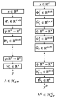
We consider a family ${\mathscr{H}}_{\sf NN}$ of $L$-layer feed-forward neural networks defined over $\mathbb{B}^{d}(r)$, with $d$ potentially very large compared to the sample size $m$. A function $h$ in ${\mathscr{H}}_{\sf NN}$ can be viewed as a cascade of linear maps composed with a non-linear activation function (see Figure 2, left column). Here, $W_{1},\ldots,W_{L}$ are the weight matrices defining the network and $\psi$ is a non-linear activation. For simplicity, the width (number of neurons) in each hidden layer, denoted by $N$, is assumed to be the same for all the layers. Also, we assume that the output of the network is a real scalar and hence we have $W_{L}\in\mathbb{R}^{N}$. Furthermore, we assume no activation in the output layer. We also assume the same activation $\psi\colon\mathbb{R}^{N}\rightarrow\mathbb{R}^{N}$ for all layers and choose it to be a sigmoid function: for any $u=(u_{1},\ldots,u_{N})\in\mathbb{R}^{N},$ $\psi(u)=(\sigma_{\eta}(u_{1}),\ldots,\sigma_{\eta}(u_{N})),$ for some $\eta>0$, where $\sigma_{\eta}(a)=\frac{1-e^{-\frac{\eta a}{2}}}{1+e^{-\frac{\eta a}{2}}}$, $a\in\mathbb{R}$. Note that $\sigma_{\eta}$ is $\eta$-Lipschitz and thus $\psi$ is $\eta$-Lipschitz with respect to $\|\cdot\|_{2}$: for any $u,v\in\mathbb{R}^{N},\|\psi(u)-\psi(v)\|_{2}\leq\eta\|u-v\|_{2}$. A typical choice for $\eta$ in practice is $\eta=1$, but we will keep the dependence on $\eta$ for generality. We define ${\mathscr{H}}_{{\sf NN}^{\Lambda}}$ as the subset of ${\mathscr{H}}_{\sf NN}$ with weight matrices that are $\Lambda$-bounded in their Frobenius norm: for all $j\in[L]$, $\|W_{j}\|_{F}\leq\Lambda$ for some $\Lambda>0$.

We design a pure DP algorithm for learning $L$-layer feed-forward networks in ${\mathscr{H}}_{{\sf NN}^{\Lambda}}$ that benefits from the following margin-based guarantee.

Theorem 5.1.

Let $\varepsilon>0,\beta\in(0,1),$ and $\rho>0$. Then, there is an $\varepsilon$-DP algorithm which returns an $L$-layer network $h^{\mathsf{Priv}}$ with $N$ neurons per layer that with probability at least $1-\beta$ over the draw of a sample $S\sim\mathscr{D}^{m}$ and the internal randomness of the algorithm admits the following guarantee:

$$R_{\mathscr{D}}(h^{\mathsf{Priv}}) \leq\min\limits_{~{}~{}~{}h\in{\mathscr{H}}_{{\sf NN}^{\Lambda}}}\widehat{R}_{S}^{\rho}(h)+O\left(\frac{r(2\eta\Lambda)^{L}\,\sqrt{N\theta}}{\rho\sqrt{m}}+\frac{r^{2}(2\eta\Lambda)^{2L}\,N\theta}{\rho^{2}\varepsilon m}\right),$$

where $\theta=\log(Lm/\beta)\log(r(\eta\Lambda)^{L}/\rho)$.

Note that this guarantee is independent of $d$ and, assuming $L$ is a constant, the bound scales roughly as $\sqrt{\frac{N}{\rho^{2}m}}+\frac{N}{\rho^{2}\varepsilon m}$, where $\rho$ is the confidence-margin parameter and $\varepsilon$ is the privacy parameter. Note that, for $\varepsilon\approx 1$, the bound scales with $\sqrt{\#\text{ neurons}}$, which is more favorable than standard bounds obtained via a uniform convergence argument, which depend on $d$, as well as the total number of edges $\Omega(N^{2})$, in addition to a similar dependence on $\Lambda^{L}$.

Our construction. Our DP learner is based on using $L$ embeddings $\Phi_{0}\in\mathbb{R}^{k\times d},\ldots,$ $\Phi_{L-1}\in\mathbb{R}^{k\times N}$ given by data-independent JL-transform matrices to reduce the dimension of the inputs in each layer, including the input layer, to $k=O\left(\frac{r^{2}(2\eta\Lambda)^{2L}}{\rho^{2}}\right)$. We randomly generate a set $\Phi=(\Phi_{0},\ldots,\Phi_{L-1})$ of $L$ independent JL matrices whose dimensions are described as above. We let ${\mathscr{H}}_{\sf NN}^{\Phi}$ denote the family of $L$-layer neural networks, where each network $h^{\Phi}\in{\mathscr{H}}^{\Phi}_{\sf NN}$ is associated with weight matrices $\Phi^{\top}_{0}\,\widetilde{W}_{1},\ldots,\Phi^{\top}_{L-1}\,\widetilde{W}_{L}$ for $\widetilde{W}_{j}\in\mathbb{R}^{k\times N},j\in[L-1]$, and $\widetilde{W}_{L}\in\mathbb{R}^{k\times 1}$ (see Figure 2, right column). We define ${\mathscr{H}}^{\Phi}_{{\sf NN}^{2\Lambda}}\subset{\mathscr{H}}^{\Phi}_{\sf NN}$ where $\|\widetilde{W}_{j}\|_{F}\leq 2\Lambda$ for all $j\in[L]$. We start by creating a $\gamma$-cover $\mathcal{C}$ of the product space of the matrices $\widetilde{W}_{1},\ldots,\widetilde{W}_{L}$ associated with ${\mathscr{H}}^{\Phi}_{{\sf NN}^{2\Lambda}}$, where $\gamma=O\left(\frac{\rho}{r(4\eta\Lambda)^{L}}\right)$. $\mathcal{C}$ is a $\gamma$-cover of $\mathbb{B}^{k\times N}(2\Lambda)\times\ldots\times\mathbb{B}^{k\times N}(2\Lambda)\times\mathbb{B}^{k}(2\Lambda)$ with respect to $\sqrt{\sum_{j=1}^{L}\|\cdot\|^{2}_{F}}$. We define $\widehat{\mathscr{H}}^{\Phi}_{{\sf NN}^{2\Lambda}}\subset{\mathscr{H}}^{\Phi}_{{\sf NN}^{2\Lambda}}$ to be the corresponding family of networks whose associated matrices are in $\mathcal{C}$. Given an input dataset $S=\left((x_{1},y_{1}),\ldots,(x_{m},y_{m})\right)\in\left(\mathbb{B}^{d}(r)\times\{\pm 1\}\right)^{m}$, we then run the exponential mechanism over $S$ with privacy parameter $\varepsilon$, the score function being the empirical zero-one loss $\widehat{R}_{S}(h)\colon h\in\widehat{\mathscr{H}}^{\Phi}_{{\sf NN}^{2\Lambda}}$, and the sensitivity $1/m$, to return a neural network $h^{\mathsf{Priv}}\in\widehat{\mathscr{H}}^{\Phi}_{{\sf NN}^{2\Lambda}}$.

6 Label Privacy Algorithms with Margin Guarantees

In many tasks, the features are public information and only the labels are sensitive and need to be protected. Several recent publications have suggested to train learning models with differential privacy for labels for these tasks, while treating features as public information [GGK⁺21, EMSV21]. This motivates the following definition of label differential privacy.

Definition 6.1 (Label differential privacy).

Let $\varepsilon,\delta\geq 0$. Let $\mathcal{A}\colon(\mathcal{X}\times\mathcal{Y})^{m}\to{\mathscr{H}}$ be a (potentially randomized) mechanism. We say that $\mathcal{A}$ is $(\varepsilon,\delta)$-label-DP if for any measurable subset $O\subset{\mathscr{H}}$ and all $S,S^{\prime}\in(\mathcal{X}\times\mathcal{Y})^{m}$ that differ in one label of one sample, the following inequality holds:

$$\operatorname*{\mathbb{P}}(\mathcal{A}(S)\in O)\leq e^{\varepsilon}\operatorname*{\mathbb{P}}(\mathcal{A}(S^{\prime})\in O)+\delta.$$ (3)

[GGK⁺21] gave an algorithm for deep learning with label differential privacy in the local differential privacy model. [YSMN21] proposed and evaluated algorithms for label differential privacy in conjunction with secure multiparty computation. [EMSV21] presented a clustering-based algorithm for label differential privacy. There are several other works which show pitfalls on label differential privacy [BFSV⁺21a, BFSV⁺21b].

Here, we design a simple algorithm for label differential privacy, which we show benefits from margin guarantees for any hypotheses class with finite fat-shattering dimension, including the class of linear classifiers, neural networks, and ensembles [BST99].

We first introduce some definitions needed to describe our algorithm. Fix $\rho>0$. Define the $\rho$-truncation function $\beta_{\rho}\colon\mathbb{R}\to[-\rho,+\rho]$ by $\beta_{\rho}(u)=\max\left\{u,-\rho\right\}1_{u\leq 0}+\min\left\{u,+\rho\right\}1_{u\geq 0}$, for all $u\in\mathbb{R}$. For any $h\in{\mathscr{H}}$, we denote by $h_{\rho}$ the $\rho$-truncation of $h$, $h_{\rho}=\beta_{\rho}(h)$, and define ${\mathscr{H}}_{\rho}=\left\{h_{\rho}\colon h\in{\mathscr{H}}\right\}$. For any family of functions ${\mathscr{F}}$, we also denote by $\mathcal{N}_{\infty}({\mathscr{F}},\varepsilon,x_{1}^{m})$ the empirical covering number of ${\mathscr{F}}$ over the sample $(x_{1},\ldots,x_{m})$ and by ${\mathscr{C}}({\mathscr{F}},\varepsilon,x_{1}^{m})$ a minimum empirical cover. With these definitions, the algorithm is given in Algorithm 4. The algorithm uses an exponential mechanism over a cover of truncated hypotheses sets.

Algorithm 4 $\mathcal{A}_{\mathsf{LabMarg}}$: Private learning algorithm under label-privacy

0:  Dataset $S=\left((x_{1},y_{1}),\ldots,(x_{m},y_{m})\right)\in\left(B^{d}\times\{\pm 1\}\right)^{m}$; privacy parameter $\varepsilon>0$; margin parameter $\rho$.

1:  Compute the $\rho/2$ minimal cover $\widehat{\mathcal{H}}_{\rho}={\mathscr{C}}({\mathscr{H}}_{\rho},\rho/2,x_{1}^{m})$.

2:  Run the Exponential mechanism with privacy parameter $\varepsilon$, sensitivity $1/m$, and score function $-\widehat{R}^{\rho/2}_{S}(h),~{}h\in\widehat{\mathcal{H}}_{\rho}$ to select $h^{\mathsf{priv}}\in\widehat{\mathcal{H}}_{\rho}$.

3:  return  $h^{\mathsf{priv}}$.

Theorem 6.1.

Algorithm 4 is $\varepsilon$-label-DP. Let $\mathscr{D}$ be a distribution on $\mathcal{X}\times\mathcal{Y}$ and suppose $S\sim\mathscr{D}^{m}$. Let $c=17$ and $d=\operatorname{fat}_{\frac{\rho}{32}}({\mathscr{H}})$ and $M=1+d\log_{2}(2c^{2}m)\log_{2}\frac{2cem}{d}+\log\frac{2}{\beta}$. For any $\beta\in(0,1)$, with probability at least $1-\beta,$ the output $w^{\mathsf{Priv}}$ satisfies:

$$R_{\mathscr{D}}(h^{\mathsf{priv}})\leq\min_{h\in{\mathscr{H}}}\left(\widehat{R}^{\rho}_{S}(h)+2\sqrt{\min_{h\in{\mathscr{H}}}\widehat{R}^{\rho}_{S}(h)}\sqrt{\frac{M}{m}}\right)+\frac{2M}{m}+\frac{64M\log\left(\frac{2}{\beta}\right)}{\varepsilon m}.$$

While our algorithm is computationally inefficient, it admits strong theoretical guarantees. First, it is an $(\varepsilon,0)$ pure label-differential privacy guarantee. Second, it is dimension-independent. Furthermore, the relative deviation margin bound it benefits from smoothly interpolates between the realizable case of $R^{\rho}_{S}(w)=0$ and the case of $R^{\rho}_{S}(w)>0$. As a corollary, note that up to constants one can always get privacy for $\varepsilon>1$ for free. Finally, observe that this bound holds not only for linear classes, but also for any hypothesis set with favorable $\rho$-fat-shattering dimension. In particular, we can use known upper bounds for the $\rho$-fat-shattering dimension of feed-forward neural networks [BST99] to derive label-privacy guarantees for training neural networks.

7 Conclusion

We presented a series of new differentially private algorithms with dimension-independent margin guarantees, including algorithms for linear classification, kernel-based classification, or learning with a family of feed-forward neural networks, and label DP learning with general hypothesis sets. Our kernel-based algorithms can be extended to non-linear classification with many other kernels, including a variety of kernels that can be approximated using polynomial kernels, using techniques based on oblivious sketching. Our study of DP algorithms with margin guarantees for a family of neural networks can be viewed as an initiatory step that could serve as the basis for a more extensive analysis of DP algorithms for broader families of neural networks.

Appendix A Useful Lemmas

We use empirical Bernstein bounds, properties of exponential mechanism and Johnson-Lindenstrauss lemmas which we state below.

Lemma A.1 (Relative deviation bound ).

For any hypothesis set ${\mathscr{H}}$ of functions mapping from $\mathcal{X}$ to $R$, with probability at least $1-\beta$, the following inequality holds for all $h\in{\mathscr{H}}$:

$$R_{\mathscr{D}}(h)\leq\widehat{R}_{S}(h)+2\sqrt{\widehat{R}_{S}(h)\frac{V({\mathscr{H}})\log(2m)+\log\frac{4}{\beta}}{m}}+4\frac{V({\mathscr{H}})\log(2m)+\log\frac{4}{\beta}}{m},$$

where $V({\mathscr{H}})$ is the VC-dimension of class ${\mathscr{H}}$.

The above lemma is obtained by combining [CGM19, Corollary 7] and VC-dimension bounds.

Lemma A.2 (Relative deviation margin bound [CMTS21]).

Fix $\rho\geq 0$. Then, for any hypothesis set ${\mathscr{H}}$ of functions mapping from $\mathcal{X}$ to $\mathbb{R}$ with $d=\operatorname{fat}_{\frac{\rho}{16}}({\mathscr{H}})$, with probability at least $1-\beta$, the following holds for all $h\in{\mathscr{H}}$:

$$R_{\mathscr{D}}(h)\leq\widehat{R}^{\rho}_{S}(h)+2\sqrt{\widehat{R}^{\rho}_{S}(h)\frac{M}{m}}+\frac{M}{m},$$

where $M=1+d\log_{2}(2c^{2}m)\log_{2}\frac{2cem}{d}+\log\frac{1}{\beta}$ and $c=17$.

Lemma A.3.

Let $\beta,\gamma\in(0,1)$. Let $T\subset\mathbb{R}^{d}$ be any set of $m$ vectors. There exists $k=O\bigg{(}\frac{\log\left(\frac{m}{\beta}\right)}{\gamma^{2}}\bigg{)}$ such that for any random $k\times d$ matrix $\Phi$ with entries drawn i.i.d. uniformly from $\{\pm\frac{1}{\sqrt{k}}\}$, the following inequalities hold simultaneously with probability at least $1-\beta$ over the choice of $\Phi$:

• For any $u\in T$,

  $$\left(1-\frac{\gamma}{3}\right)\|u\|_{2}^{2}\leq \|\Phi u\|_{2}^{2}\leq\left(1+\frac{\gamma}{3}\right)\|u\|_{2}^{2}.$$

• For any $u,v\in T$,

  $$\lvert\langle\Phi u,\Phi v\rangle -\langle u,v\rangle\rvert\leq\frac{\gamma}{3}\,\|u\|_{2}\,\|v\|_{2}.$$

Proof.

The first property is simply the Johnson-Lindenstrauss (JL) property and follows from the standard JL lemma (see, e.g., [JL84, LN17]). Below we show both first and second property holds simultaneously. Define

$$\widetilde{T}\triangleq\left\{z\in\mathbb{R}^{d}:~{}z=\frac{u}{\|u\|_{2}}\pm\frac{v}{\|v\|_{2}},~{}u,v\in T\right\}.$$

Note that the number of non-zero vectors in $\widetilde{T}$ is at most $m^{2}$. By the JL lemma [JL84, LN17] over the set $T\cup\widetilde{T}$, there exists $k=O\left(\frac{\log(m^{2}/\beta)}{\gamma^{2}}\right)=O\left(\frac{\log\left(\frac{m}{\beta}\right)}{\gamma^{2}}\right)$ and $\Phi^{\prime}$ such that with probability $\geq 1-\beta$, for all $u,v\in T$ we have

$$\left(1-\frac{\gamma}{3}\right)\|\bar{u}+\bar{v}\|_{2}^{2}\leq \|\Phi^{\prime}(\bar{u}+\bar{v})\|_{2}^{2}\leq\left(1+\frac{\gamma}{3}\right)\|\bar{u}+\bar{v}\|_{2}^{2},$$ (4)

$$\left(1-\frac{\gamma}{3}\right)\|\bar{u}-\bar{v}\|_{2}^{2}\leq \|\Phi^{\prime}(\bar{u}-\bar{v})\|_{2}^{2}\leq\left(1+\frac{\gamma}{3}\right)\|\bar{u}-\bar{v}\|_{2}^{2},$$ (5)

$$\left(1-\frac{\gamma}{3}\right)\|u\|_{2}^{2}\leq \|\Phi^{\prime}u\|_{2}^{2}\leq\left(1+\frac{\gamma}{3}\right)\|u\|_{2}^{2}.$$ (6)

where $\bar{u}=\frac{u}{\|u\|_{2}}$ and $\bar{v}=\frac{v}{\|v\|_{2}}$. (6) implies the first result in the lemma. Now, fix any $u,v\in T$. Let $\bar{u}=\frac{u}{\|u\|_{2}}$ and $\bar{v}=\frac{v}{\|v\|_{2}}$. Observe that for any $\mathbf{a},\mathbf{b}\in\mathbb{R}^{d}$, we have $\langle\mathbf{a},\mathbf{b}\rangle=\frac{1}{4}\left(\|\mathbf{a}+\mathbf{b}\|_{2}^{2}-\|\mathbf{a}-\mathbf{b}\|_{2}^{2}\right)$. Hence, we have

$$\big{\lvert}\langle\bar{u},\bar{v}\rangle-\langle\Phi^{\prime}\bar{u},\Phi^{\prime}\bar{v}\rangle\big{\rvert} \leq\frac{1}{4}\big{\lvert}\|\bar{u}+\bar{v}\|^{2}_{2}-\|\Phi^{\prime}(\bar{u}+\bar{v})\|^{2}_{2}\big{\rvert}+\frac{1}{4}\big{\lvert}\|\Phi^{\prime}(\bar{u}-\bar{v})\|^{2}_{2}-\|\bar{u}-\bar{v}\|^{2}_{2}\big{\rvert}$$ ( )

$$\leq\frac{\gamma}{12}\left(\|\bar{u}+\bar{v}\|^{2}_{2}+\|\bar{u}-\bar{v}\|^{2}_{2}\right)$$

$$\leq\frac{\gamma}{3},$$

where the second inequality follows from (4) and (5) ’and the third inequality follows from the triangle inequality and the fact that $\|\bar{u}\|_{2}=\|\bar{v}\|_{2}=1$. Hence, we finally have

$$\lvert\langle u,v\rangle-\langle\Phi^{\prime}u,\Phi^{\prime}v\rangle\rvert\leq\|u\|_{2}\|v\|_{2}\,\lvert\langle\bar{u},\bar{v}\rangle-\langle\Phi^{\prime}\bar{u},\Phi^{\prime}\bar{v}\rangle\rvert\leq\frac{\gamma}{3}\|u\|_{2}\|v\|_{2}.$$

∎

The time complexity to apply the random matrix $\Phi$ in Lemma A.3 to a vector $v$ is $k\cdot d$, which can be prohibitive in many cases. There are several works which provide $\Phi$ that support fast matrix vector products. [AC06] provides a $\Phi$ which can be applied in time $c^{\prime}d\log d+\frac{c^{\prime}\log(d/\beta)\log^{2}(1/\beta)}{\gamma^{2}}$, however the results are stated with constant probability. [Nel10] gave a slightly different construction which can be applied in time $c^{\prime}d\log d+\frac{c^{\prime}\log(d/\beta)\log^{2}(1/\beta)}{\gamma^{4}}$ and the results hold with high probability. [AL09] provided a construction which can be applied in time $c^{\prime}d\log k$ for $k=O(d^{0.499})$. [KW11] showed that any RIP matrix can be used for JL-transform and provided JL-transform results for several fast random projections. Since we need high probability bounds without any restrictions, we use the following result, which is computationally efficient, but is suboptimal in the projection dimension up to logarithmic factors.

Lemma A.4.

Let $\beta,\gamma\in(0,1)$ and $c$ and $c^{\prime}$ be sufficiently large constants. Let $T\subset\mathbb{R}^{d}$ be any set of $m$ vectors. Let $k=\frac{c\log\left(\frac{m}{\beta}\right)\log\left(\frac{m}{\gamma\beta}\right)}{\gamma^{2}}$. There exists a matrix $\Phi$ which can be applied to any vector $v$ in time $c^{\prime}d\log d+c^{\prime}k$, such that the following inequalities hold simultaneously with probability at least $1-\beta$ over the choice of $\Phi$:

• For any $u\in T$,

  $$\left(1-\frac{\gamma}{3}\right)\|u\|_{2}^{2}\leq \|\Phi u\|_{2}^{2}\leq\left(1+\frac{\gamma}{3}\right)\|u\|_{2}^{2}.$$ (7)

• For any $u,v\in T$,

  $$\lvert\langle\Phi u,\Phi v\rangle -\langle u,v\rangle\rvert\leq\frac{\gamma}{3}\,\|u\|_{2}\,\|v\|_{2}.$$ (8)

Property (7) in the above result follows directly from [Nel15] and the proof for property (8) is similar to that of Lemma A.3 and is omitted.

Appendix B DP Algorithms for Linear Classification with Margin Guarantees

B.1 Proof of Theorem 3.1

See 3.1

Proof.

The proof of privacy follows from combining the following two properties: $\tilde{w}$ is generated via the exponential mechanism, which an $\varepsilon$-differentially private mechanism, and $\Phi$ is generated independently of $S$.

We now prove the accuracy guarantee of Algorithm 1. If $m<\frac{c\Lambda^{2}r^{2}\log\left(\frac{m}{\beta}\right)\log\left(\frac{20\Lambda r}{\beta\rho}\right)}{\rho^{2}\varepsilon}$, for some constant $c$, the bound follow trivially. Hence in the rest of the proof we assume that $m$ is at least $\frac{c\Lambda^{2}r^{2}\log\left(\frac{m}{\beta}\right)\log\left(\frac{20\Lambda r}{\beta\rho}\right)}{\rho^{2}\varepsilon}$ for some large constant $c$. Let

$$\alpha=\frac{c\Lambda^{2}r^{2}\log\left(\frac{m}{\beta}\right)\log\left(\frac{20\Lambda r}{\beta\rho}\right)}{\rho^{2}\varepsilon m}.$$

First, observe that

$$\widehat{R}_{S}(w^{\mathsf{Priv}}) =\frac{1}{m}\sum_{(x,y)\in S}\mathbf{1}\left(y\langle w^{\mathsf{Priv}},x\rangle\right)$$

$$=\frac{1}{m}\sum_{(x,y)\in S}\mathbf{1}\left(y\langle\Phi^{\top}\tilde{w},x\rangle\right)$$

$$=\frac{1}{m}\sum_{(x,y)\in S}\mathbf{1}\left(y\langle\tilde{w},\Phi x\rangle\right)$$

$$=\frac{1}{m}\sum_{(x_{\Phi},y)\in S_{\Phi}}\mathbf{1}\left(y\langle\tilde{w},x_{\Phi}\rangle\right)$$

$$=\widehat{R}^{(k)}_{S_{\Phi}}(\tilde{w}).$$

Let $\widehat{w}\in\operatorname*{argmin}\limits_{w\in\mathcal{C}}\widehat{R}^{(k)}_{S_{\Phi}}(w)$. Note that $\lvert\mathcal{C}\rvert=\left(\frac{20\,\Lambda\,r}{\rho}\right)^{k}$, where $k=\frac{c^{\prime}\,\Lambda^{2}\,r^{2}\,\log\left(\frac{m}{\beta}\right)}{\rho^{2}}$. Hence, by the accuracy properties of the exponential mechanism and the fact that $m\geq\frac{4\log\left(\frac{4\lvert\mathcal{C}\rvert}{\beta}\right)}{\varepsilon\alpha}$, we have that with probability at least $1-\beta/4$,

$$\widehat{R}^{(k)}_{S_{\Phi}}(\tilde{w}) \leq\widehat{R}^{(k)}_{S_{\Phi}}(\widehat{w})+\alpha.$$

Combining the above facts, we get that with probability at least $1-\beta/4$,

$$\widehat{R}_{S}(w^{\mathsf{Priv}}) \leq\widehat{R}^{(k)}_{S_{\Phi}}(\widehat{w})+\alpha.$$ (9)

Let $w^{\ast}\in\operatorname*{argmin}\limits_{w\in\mathbb{B}^{d}(\Lambda)}\widehat{R}^{\rho}_{S}(w)$ and let $w^{\ast}_{\Phi}=\Phi w^{\ast}$. Note that

$$\|w^{\ast}_{\Phi}\|_{2}\leq\sqrt{1+\frac{\rho}{3\Lambda r}}\|w^{\ast}\|_{2}\leq 2\|w^{\ast}\|_{2}\leq 2\Lambda,$$

and hence $w^{\ast}_{\Phi}\in\mathbb{B}^{k}(2\Lambda)$. Since $\mathcal{C}$ is $\frac{\rho}{10\,r}$-cover of $\mathbb{B}^{k}(2\Lambda)$, then there must be $w_{c}\in\mathcal{C}$ such that $\|w_{c}-w^{\ast}_{\Phi}\|_{2}\leq\frac{\rho}{10\,r}$. Hence, observe that for any $(x_{\Phi},y)\in S_{\Phi}$,

$$y\langle w_{c},x_{\Phi}\rangle =y\langle w^{\ast}_{\Phi},x_{\Phi}\rangle+y\langle w_{c}-w^{\ast}_{\Phi},x_{\Phi}\rangle$$

$$\geq y\langle w^{\ast}_{\Phi},x_{\Phi}\rangle-\|w_{c}-w^{\ast}_{\Phi}\|_{2}\,\|x_{\Phi}\|_{2}$$

$$\geq y\langle w^{\ast}_{\Phi},x_{\Phi}\rangle-\frac{\rho}{10\,r}\|x_{\Phi}\|_{2}.$$

Now, by Lemma A.3, with probability at least $1-\beta/4$, for all $x_{\Phi}$ s.t. $(x_{\Phi},y)\in S_{\Phi}$ we have $\|x_{\Phi}\|_{2}\leq\sqrt{1+\frac{\rho}{3\Lambda r}}\|x\|_{2}\leq\sqrt{1+\frac{\rho}{3\Lambda r}}r$. Hence, we get that with probability at least $1-\beta/4$ for all $(x_{\Phi},y)\in S_{\Phi}$

$$y\langle w_{c},x_{\Phi}\rangle \geq y\langle w^{\ast}_{\Phi},x_{\Phi}\rangle-0.15\rho.$$

The last inequality implies that for any $\rho^{\prime}>0$, with probability at least $1-\beta/4$ (over the choice of $\Phi$), we must have $\widehat{R}^{\rho^{\prime},(k)}_{S_{\Phi}}(w_{c})\leq\widehat{R}^{\rho^{\prime}+0.15\rho,(k)}_{S_{\Phi}}(w^{\ast}_{\Phi})$. In particular, with probability at least $1-\beta/4$ we have

$$\widehat{R}^{0.5\rho,(k)}_{S_{\Phi}}(w_{c}) \leq\widehat{R}^{0.65\rho,(k)}_{S_{\Phi}}(w^{\ast}_{\Phi}).$$ (10)

Moreover, by the definition of $\widehat{w}$, we have $\widehat{R}^{(k)}_{S_{\Phi}}(\widehat{w})\leq\widehat{R}^{(k)}_{S_{\Phi}}(w_{c})\leq\widehat{R}^{0.5\rho,(k)}_{S_{\Phi}}(w_{c})$. Combining this fact with (9) and (10), we get that with probability at least $1-\beta/2$

$$\widehat{R}_{S}(w^{\mathsf{Priv}}) \leq\widehat{R}^{0.65\rho,(k)}_{S_{\Phi}}(w^{\ast}_{\Phi})+\alpha.$$ (11)

Now, by Lemma A.3 and the fact that $\|w^{\ast}\|_{2}\leq\Lambda$ and $\|x\|_{2}\leq r$, it follows that with probability at least $1-\beta/4$ for all $(x_{\Phi},y)\in S_{\Phi}$, we have

$$y\langle w^{\ast},x\rangle\geq\rho\implies y\langle w^{\ast}_{\Phi},x_{\Phi}\rangle\geq\rho/3.$$

This directly implies that with probability at least $1-\beta/4$,

$$\widehat{R}^{0.65\rho,(k)}_{S_{\Phi}}(w^{\ast}_{\Phi}) \leq\widehat{R}^{\rho}_{S}(w^{\ast}).$$

Combining this with (11), we can assert that with probability at least $1-\frac{3}{4}\beta$, we have

$$\widehat{R}_{S}(w^{\mathsf{Priv}}) \leq\widehat{R}^{\rho}_{S}(w^{\ast})+\alpha.$$ (12)

In the final step of the proof, we rely on a standard uniform convergence argument to bound $R_{\mathscr{D}}(w^{\mathsf{Priv}})$ in terms of $\widehat{R}_{S}(w^{\mathsf{Priv}})$. Note that the VC-dimension of $\left\{\operatorname*{sgn}\circ h_{w}:w\in\mathcal{C}\right\}$ is $k$. By Lemma A.1, with probability at least $1-\beta/4$

$$R_{\mathscr{D}}(w^{\mathsf{Priv}})-\widehat{R}_{S}(w^{\mathsf{Priv}})\leq 2\sqrt{\widehat{R}_{S}(w^{\mathsf{Priv}})\frac{k\log(2m)+\log({16}/{\beta})}{m}}+4\frac{k\log(2m)+\log({16}/{\beta})}{m}.$$

Combining the above two equations, we get with probability at least $1-\beta$,

$$R_{\mathscr{D}}(w^{\mathsf{Priv}})\leq\widehat{R}^{\rho}_{S}(w^{\ast})+2\sqrt{\widehat{R}^{\rho}_{S}(w^{\ast})\frac{k\log(2m)+\log({16}/{\beta})}{m}}+2\alpha+8\frac{k\log(2m)+\log({16}/{\beta})}{m}.$$

The lemma follows from observing that $w^{\ast}\in\operatorname*{argmin}\limits_{w\in\mathbb{B}^{d}(\Lambda)}\widehat{R}^{\rho}_{S}(w)$ if and only if $w^{\ast}\in\operatorname*{argmin}\limits_{w\in\mathbb{B}^{d}(\Lambda)}\widehat{R}^{\rho}_{S}(w)+2\sqrt{\widehat{R}^{\rho}_{S}(w)\frac{k\log(2m)+\log({16}/{\beta})}{m}}$. ∎

B.2 Algorithm 5 of Section 3.2 and Proof of Lemma 3.1

Here, we give the details of Algorithm 5 invoked in step 4 of Algorithm 2. We describe here a more general setup where the loss function is any (possibly non-smooth) convex generalized linear loss (GLL). Given a parameter space $\mathcal{W}$, feature space $\mathcal{X}$, and label/target set $\mathcal{Y}$, a GLL is a loss function defined over $\mathcal{W}\times(\mathcal{X}\times\mathcal{Y})$ that can be written as $\ell(\langle w,x\rangle,y),~{}w\in\mathcal{W},x\in\mathcal{X},y\in\mathcal{Y}$ for some function $\ell:\mathbb{R}\times\mathcal{Y}\rightarrow\mathbb{R}$. Here, we assume that for any $y\in\mathcal{Y}$, $\ell(\cdot,y)$ is convex and $\frac{1}{\rho}$-Lipschitz. We also assume that $\mathcal{W}\subseteq\mathbb{B}^{k}(\Lambda)$ for some $\Lambda>0$, $\mathcal{X}\subseteq\mathbb{B}^{k}(\tilde{r})$ for some $\tilde{r}>0$, and $\mathcal{Y}\subseteq[-1,1]$. Given a dataset $\widetilde{S}=((x_{1},y_{1}),\ldots,(x_{m},y_{m}))\in(\mathcal{X}\times\mathcal{Y})^{m}$, we define the empirical risk of $w\in\mathcal{W}$ with respect to $\widetilde{S}$ as $\widehat{L}_{\widetilde{S}}(w)\triangleq\frac{1}{m}\sum_{i=1}^{m}\ell(\langle w,x_{i}\rangle,y)$. Note that the setup in Algorithm 2 is a special case of the above.

Given an input dataset $\widetilde{S}\in(\mathcal{X}\times\mathcal{Y})^{m}$, Algorithm 5 below invokes the “Phased SGD algorithm for GLL” [BGM21, Algorithm 2] on a set $\widehat{S}$ of $m$ samples drawn uniformly with replacement from $\widetilde{S}$, and hence obtain an output $\tilde{w}\in\mathcal{W}$. In the sequel, we will refer to the algorithm in [BGM21] as $\mathcal{A}_{\sf GLL}$. Note that the expected loss with respect to the choice of $\widehat{S}\leftarrow\widetilde{S}$ is the empirical risk with respect to $\widetilde{S}$. Hence, one can derive a bound on the expected excess empirical risk that is roughly the same as the bound in [BGM21, Theorem 6] on the expected excess population risk. However, we note that ensuring that Algorithm 5 is $(\varepsilon,\delta)$-DP does not follow directly from the privacy guarantee of the $\mathcal{A}_{\sf GLL}$ since the sample $\widehat{S}$ may contain duplicate entries from $\widetilde{S}$. Nonetheless, we show that the privacy guarantee can be attained by appropriately setting the input privacy parameters to $\mathcal{A}_{\sf GLL}$ together with a careful privacy analysis. To transform the in-expectation bound into a high-probability bound, we perform a standard confidence-boosting procedure [BST14, Appendix D], where the procedure described above is repeated independently $M=O(\log(1/\beta))$ times to generate $\tilde{w}^{1},\ldots,\tilde{w}^{M}$, and finally, the exponential mechanism (with a score function $-\widehat{L}_{\widetilde{S}}$) is used to privately select a final output $\tilde{w}\in\{\tilde{w}^{1},\ldots,\tilde{w}^{M}\}$.

Algorithm 5 DP-ERM algorithm for GLLs

0:  Private dataset $\widetilde{S}=\big{(}(x_{1},y_{1}),\dots,(x_{m},y_{m})\big{)}\in(\mathcal{X}\times\mathcal{Y})^{m}$, where $\mathcal{X}\subseteq\mathbb{B}^{k}(\tilde{r})$ and $\mathcal{Y}\subseteq[-1,1]$; parameter space $\mathcal{W}\subseteq\mathbb{B}^{k}(\Lambda)$; privacy parameters $(\varepsilon,\delta)$; confidence parameter $\beta\in(0,1)$; convex, $\frac{1}{\rho}$-Lipschitz loss function $\ell$ for some $\rho>0$; Oracle access to algorithm $\mathcal{A}_{\sf GLL}$ [BGM21, Algorithm 2].

1:  Let $M:=\log(2/\beta)$.

2:  Let $\varepsilon^{\prime}:=\frac{\varepsilon}{4M\log(2M/\delta)}$.

3:  Let $\delta^{\prime}:=\frac{\delta^{2}}{4M\log(2M/\delta)}$.

4:  for $t=1$ to $M$ do

5:     Sample $\widehat{S}^{t}=\big{(}(\widehat{x}^{t}_{1},\widehat{y}^{t}_{1}),\ldots\big{(}\widehat{x}^{t}_{m},\widehat{y}^{t}_{m}\big{)}\big{)}\leftarrow\widetilde{S}$ uniformly with replacement.

6:     $\tilde{w}^{t}=\mathcal{A}_{\sf GLL}(\widehat{S}^{t};\varepsilon^{\prime},\delta^{\prime})$, where $\mathcal{A}_{\sf GLL}$ is [BGM21, Algorithm 2] (the other obvious inputs to $\mathcal{A}_{\sf GLL}$ are omitted; the smoothing parameter and the oracle accuracy parameter of $\mathcal{A}_{\sf GLL}$ are set as in [BGM21, Theorem 6]).

7:  end for

8:  Run the exponential mechanism with privacy parameter $\varepsilon/2$ to select $\tilde{w}$ from the set $\big{(}\tilde{w}^{1},\ldots,\tilde{w}^{M}\big{)}$ associated with scores $\big{(}-\widehat{L}_{\widetilde{S}}(\tilde{w}^{t}):~{}t\in[M]\big{)}$.

9:  return  $\tilde{w}$

See 3.1

Proof.

First, we show the privacy guarantee. Fix a round $t\in[M]$ of Algorithm 5. We will show that the $t$-th round is $(\frac{\varepsilon}{2M},\frac{\delta}{M})$-DP. Suppose we can do that. Then, by the basic composition property of DP, the entire $M$ rounds of the algorithm is $(\frac{\varepsilon}{2},\delta)$-DP. Next, we note that step 8 is $(\frac{\varepsilon}{2},0)$-DP by the privacy guarantee of the exponential mechanism. Hence, again by basic composition of DP, we conclude that Algorithm 5 is $(\varepsilon,\delta)$-DP. Thus, it remains to show that for any fixed $t\in[M]$, the $t$-th round is $(\hat{\varepsilon},\hat{\delta})$-DP, where $\hat{\varepsilon}=\frac{\varepsilon}{2M}$ and $\hat{\delta}=\frac{\delta}{M}$. Fix any data point $(x_{i},y_{i})\in\widetilde{S}$. Let $J$ denote the number of appearances of $(x_{i},y_{i})$ in $\widehat{S}^{t}$. Note that $J\sim\mathsf{Bin}(m,1/m)$. Hence, using the multiplicative Chernoff’s bound, $J\leq 2\log(2/\hat{\delta})$ with probability at least $1-\hat{\delta}/2$. We will show that conditioned on this event, the $t$-th round is $(\hat{\varepsilon},\hat{\delta}/2)$-DP, which suffices to prove our privacy claim for round $t$. Given that $J\leq 2\log(2/\hat{\delta})$ and since $\mathcal{A}_{\sf GLL}$ is $(\frac{\hat{\varepsilon}}{2\log(2/\hat{\delta})},\frac{\delta\hat{\delta}}{4\log(2/\hat{\delta})})$-DP with respect to to its input dataset $\widehat{S}^{t}$, then by the group-privacy property of DP [DR14], round $t$ is $(\hat{\varepsilon},\delta^{\prime\prime})$-DP with respect to the dataset $\widetilde{S}$, where

$$\delta^{\prime\prime} =\frac{\delta\hat{\delta}}{4\log(2/\hat{\delta})}\cdot\sum_{j=0}^{2\log(2/\hat{\delta})}e^{\frac{\hat{\varepsilon}}{2\log(2/\hat{\delta})}\,j}$$

$$=\frac{\delta\hat{\delta}}{4\log(2/\hat{\delta})}\cdot\frac{e^{\hat{\varepsilon}}-1}{e^{\frac{\hat{\varepsilon}}{2\log(2/\hat{\delta})}}-1}$$

$$\leq\frac{\delta\hat{\delta}\left(e^{\hat{\varepsilon}}-1\right)}{2\hat{\varepsilon}}$$

$$\leq\frac{\hat{\delta}}{2},$$

where the third inequality follows from the fact that $e^{\frac{\hat{\varepsilon}}{2\log(2/\hat{\delta})}}-1\geq\frac{\hat{\varepsilon}}{2\log(2/\hat{\delta})}$, and the last step follows from the fact that $\frac{e^{a}-1}{a}$ is increasing in $a>0$ and the assumption that $\varepsilon\leq\log(1/\delta)$ (and hence $\hat{\varepsilon}<\varepsilon\leq\log(1/\delta)$). Hence, we have shown that any given round of the algorithm is $(\varepsilon,\hat{\delta})$-DP. This concludes the proof of the privacy guarantee.

We now prove the bound on the excess empirical risk. Fix any round $t$. Let $\widehat{\mathscr{D}}_{\widetilde{S}}$ denote the empirical distribution of $\widetilde{S}$. Note that $\widehat{S}^{t}\sim\widehat{\mathscr{D}}_{\widetilde{S}}^{m}$, i.e., $\widehat{S}^{t}$ is comprised of $m$ independent samples from $\widehat{\mathscr{D}}_{\widetilde{S}}$. Hence, $\underset{(x,y)\sim\widehat{\mathscr{D}}_{\widetilde{S}}}{\mathbb{E}}\left[\ell(\langle w,x\rangle,y)\right]=\widehat{L}_{\widetilde{S}}(w)$. Thus, by the excess risk guarantee of $\mathcal{A}_{\sf GLL}$ [BGM21, Theorem 6], we have

$$\underset{}{\mathbb{E}}\left[\widehat{L}^{\rho}_{\widetilde{S}}(\tilde{w})\right]-\min\limits_{w\in\mathbb{B}^{k}(\Lambda)}\widehat{L}^{\rho}_{\widetilde{S}}(w) =\frac{\Lambda\tilde{r}}{\rho}\cdot O\left(\frac{1}{\sqrt{m}}+\frac{\sqrt{k\log(\frac{1}{\delta^{\prime}})}}{\varepsilon^{\prime}m}\right)$$

$$=\frac{\Lambda\tilde{r}}{\rho}\cdot O\left(\frac{1}{\sqrt{m}}+\frac{\sqrt{k}\log^{\frac{3}{2}}(\frac{1}{\delta})\log(\frac{1}{\beta})}{\varepsilon m}\right),$$

where the expectation is with respect to the sampling step (step 5 of Algorithm 5) and the randomness in $\mathcal{A}_{\sf GLL}$. Note the last step follows from the setting of $\varepsilon^{\prime}$ and $\delta^{\prime}$ in Algorithm 5 and the fact that $\log\left(\log(1/\beta)/\delta\right)=O(\log(1/\delta))$, which follows from the assumption $\delta<1/m$ (in the statement of the lemma) and $\log(1/\beta)<m$ (since the bound would be trivial otherwise). Given this expectation guarantee on the output of each round, the final selection step (step 8) returns a parameter $\tilde{w}$ that satisfies the bound above with probability at least $1-\beta$. This can be shown by following the same argument in [BST14, Appendix D] while noting that the sensitivity of the score function $-\widehat{L}_{\widetilde{S}}$ is bounded by $\frac{\Lambda\tilde{r}}{m}$.

Finally, the running time of $\mathcal{A}_{\sf GLL}$, measured in terms of gradient computations, is $O(m\log(m))$ [BGM21, Theorem 6]. Hence, the gradient complexity of Algorithm 5 is bounded by $O(m\log(m)\log(1/\beta))$. ∎

B.3 Proof of Theorem 3.2

See 3.2

Proof.

The proof of privacy follows directly from the $(\varepsilon,\delta)$-DP guarantee of Algorithm 5 (step 4) and the fact that DP is closed under post-processing.

Next, we will prove the claimed margin bound. For simplicity and without loss of generality, we will set $\Lambda=1$. For the general setting of $\Lambda$, the claimed bound follows by rescaling the parameter vectors in the proof.

Recall that $x_{\Phi}\triangleq\Phi x$. Let $w^{\ast}\in\operatorname*{argmin}\limits_{w\in\mathbb{B}^{d}}\widehat{L}^{\rho}_{S}(w)$. Define $w^{\ast}_{\Phi}\triangleq\Phi w^{\ast}$. By Lemma A.4, there is $\gamma=O\left(\sqrt{\frac{\log\left(\frac{m}{\beta}\right)}{k}}\right)=O\left(\sqrt{\frac{\log(1/\beta)}{\varepsilon m}}\log^{\frac{3}{4}}(1/\delta)\right)$ such that with probability at least $1-\beta/3$ over the randomness of $\Phi$, for every feature vector $x$ in the training set $S$, we have

$$\|x_{\Phi}\|_{2}^{2} \leq\left(1+\frac{\gamma}{3}\right)\|x\|_{2}^{2}$$ (13)

$$1-\frac{y\langle w^{\ast}_{\Phi},x_{\Phi}\rangle}{\rho} \leq 1-\frac{y\langle w^{\ast},x\rangle}{\rho}+\frac{r\gamma}{\rho}$$ (14)

We condition on this event for the remainder of the proof.

Note that (13) implies that

$$S_{\Phi}=\{(x_{\Phi},y):(x,y)\in S\};$$

that is, for all feature vectors $x$ in the dataset $S$, $x_{\Phi}\in\mathbb{B}^{k}(2r)$ (i.e., $\Pi_{\mathbb{B}^{k}(2r)}(x_{\Phi})=x_{\Phi}$).

Let $\mathscr{D}_{\Phi}$ denote the distribution of the pair $(x_{\Phi},y)$, where $(x,y)\sim\mathscr{D}$. Via a standard margin bound [MRT18, Theorems 5.8 & 5.10], with probability at least $1-\beta/3$ over the choice of the training set $S$, we have

$$\forall w\in\mathbb{B}^{k}~{}\quad~{}R_{\mathscr{D}_{\Phi}}(w) \leq\widehat{L}^{\rho}_{S_{\Phi}}(w)+\frac{4r}{\rho\sqrt{m}}+2\sqrt{\frac{\log(6/\beta)}{m}}$$

It follows that with probability at least $1-\beta/3$, we have

$$R_{\mathscr{D}_{\Phi}}(\tilde{w}) \leq\widehat{L}^{\rho}_{S_{\Phi}}(\tilde{w})+\frac{4r}{\rho\sqrt{m}}+2\sqrt{\frac{\log(6/\beta)}{m}},$$

where $\tilde{w}$ is the output of step 4 of Algorithm 2. Moreover, note that

$$R_{\mathscr{D}}(w^{\mathsf{Priv}}) =\underset{(x,y)\sim\mathscr{D}}{\mathbb{P}}\left[y\langle w^{\mathsf{Priv}},x\rangle\leq 0\right]$$

$$=\underset{(x_{\Phi},y)\sim\mathscr{D}_{\Phi}}{\mathbb{P}}\left[y\langle\tilde{w},x_{\Phi}\rangle\leq 0\right]$$

$$=R_{\mathscr{D}_{\Phi}}(\tilde{w})$$

Thus, we get that with probability at least $1-\beta/3$,

$$R_{\mathscr{D}}(w^{\mathsf{Priv}}) \leq\widehat{L}^{\rho}_{S_{\Phi}}(\tilde{w})+\frac{4r}{\rho\sqrt{m}}+2\sqrt{\frac{\log(6/\beta)}{m}}.$$ (15)

By Lemma 3.1, with probability at least $1-\beta/3$ over the randomness of Algorithm 5 (step 4 of Algorithm 2), we have that

$$\widehat{L}^{\rho}_{S_{\Phi}}(\tilde{w}) \leq\widehat{L}^{\rho}_{S_{\Phi}}(\widehat{w})+\frac{\Lambda r}{\rho}\left(\frac{1}{\sqrt{m}}+\frac{\sqrt{\log(\frac{m}{\beta})\log(\frac{1}{\beta})}\log^{\frac{3}{4}}(\frac{1}{\delta})}{\sqrt{\varepsilon m}}\right),$$ (16)

where $\widehat{w}\in\operatorname*{argmin}\limits_{w\in\mathbb{B}^{k}}\widehat{L}^{\rho}_{S_{\Phi}}(w)$. Moreover, (14) implies

$$\widehat{L}^{\rho}_{S_{\Phi}}(w^{\ast}_{\Phi}) \leq\widehat{L}^{\rho}_{S}(w^{\ast})+\frac{r}{\rho}\cdot O\left(\sqrt{\frac{\log(1/\beta)}{\varepsilon m}}\log^{\frac{3}{4}}(1/\delta)\right)$$

Note that by definition of $\widehat{w}$, we have $\widehat{L}^{\rho}(\widehat{w};S)\leq\widehat{L}^{\rho}_{S_{\Phi}}(w^{\ast}_{\Phi})$. Hence, we have

$$\widehat{L}^{\rho}_{S_{\Phi}}(\widehat{w}) \leq\widehat{L}^{\rho}_{S}(w^{\ast})+\frac{r}{\rho}O\left(\sqrt{\frac{\log(1/\beta)}{\varepsilon m}}\log^{\frac{3}{4}}(1/\delta)\right)$$ (17)

Now, by combining (15), (16), and (17), we reach the desired bound.

Finally, concerning the running time, observe that the Fast JL-transform (steps 2 and 3) takes $O(md\log(d)+\varepsilon m^{2}\log(m)/\log^{3/2}(1/\delta))$ (follows from Lemma A.4), the DP-ERM algorithm (Algorithm 5) invoked in step 4 has $O(m)$ gradient steps; each of which takes involves $O(k+\log(m))=O(\varepsilon m\log(m)/\log^{3/2}(1/\delta))$ operations. That is, the total number of operations of this step is $O(\varepsilon m^{2}\log(m)/\log^{3/2}(1/\delta))$. Finally, the step 5 requires $O(dk)=O(\varepsilon dm\log(m)/\log^{3/2}(1/\delta))$. Thus, the overall running time is $O\left(md\log\left(\max(d,m)\right)+\varepsilon m^{2}\log(m)/\log^{\frac{3}{2}}(1/\delta)\right)$.

∎

Appendix C DP Algorithms for Kernel-Based Classification with Margin Guarantees

See 4.2

Proof.

Let $S_{\widehat{\psi}}$ be as defined in step 4 in Algorithm 3. Note that by Theorem 4.1, we have $\|\widehat{\psi}(x_{i})\|_{2}=r$ for all $i\in[m]$. Moreover, the output of Algorithm 3 depends only on $S_{\widehat{\psi}}$. Thus, the privacy guarantee follows directly from the privacy guarantee of Algorithm 2 (Theorem 3.2).

Next, we turn to proving the claimed margin bound. First, note that using the margin bound attained by Algorithm 2 (Theorem 3.2), it follows that for any fixed realization of the randomness in $\widehat{\psi}$, with probability $1-\beta/2$ over the choice of $S\sim\mathcal{D}^{m}$ and the internal randomness of Algorithm 2, we have

$$R_{\mathscr{D}}(h^{\widehat{\psi}}_{w^{\mathsf{Priv}}}) \leq\min\limits_{w\in\mathbb{B}^{2D}\,(2\Lambda)}\widehat{L}^{\rho}_{S_{\widehat{\psi}}}(w)+O\left(\sqrt{\frac{\log(1/\beta)}{m}}+\frac{\Lambda r}{\rho}\left(\frac{1}{\sqrt{m}}+\frac{\sqrt{\log(\frac{m}{\beta})\log(\frac{1}{\beta})}\log^{\frac{3}{4}}(\frac{1}{\delta})}{\sqrt{\varepsilon m}}\right)\right).$$ (18)

The essence of the proof is to show that with probability $\geq 1-\beta/2$ over the randomness in $\widehat{\psi}$ (i.e., over the choice of $\omega_{1},\ldots,\omega_{D}$), we have

$$\min\limits_{w\in\mathbb{B}^{2D}\,(2\Lambda)}\widehat{L}^{\rho}_{S_{\widehat{\psi}}}(w) \leq\min\limits_{h\in\mathcal{H}_{\Lambda}}\widehat{L}^{\rho}_{S}(h)+\frac{2\Lambda r}{\rho\sqrt{m}}.$$ (19)

Combining (18) and (19) yields the desired bound.

To prove the bound in (19), we will use the following fact. .

Fact C.1.

Let $\mu>0$. Let $\psi\colon\mathcal{X}\to\mathbb{R}$ denote the feature map associated with the kernel $K$. Let $h_{\mu}=\operatorname*{argmin}_{h\in\mathcal{H}_{\Lambda}}\left(\widehat{L}^{\rho}_{S}(h)+\mu\|h\|^{2}_{\,\mathbb{H}}\right)$. Then, $h_{\mu}=\sum_{i=1}^{m}\alpha_{i}\psi(x_{i})$ for some $\alpha_{i}$, $i\in[m]$, that satisfy: $0\leq y_{i}\alpha_{i}\leq\frac{1}{2\,m\,\mu\,\rho}$.

This fact simply follows from the dual formulation of the optimization problem for kernel support vector machines (see, e.g., [MRT18, Section 6.3]) . The fact asserts that the minimizer $h_{\mu}$ of the regularized empirical hinge loss can be expressed as a linear combination of $(\psi(x_{i}):i\in[m])$ (such assertion also follows from the representer theorem) where the coefficients of the linear combination (the dual variables) $\alpha=(\alpha_{1},\ldots,\alpha_{m})$ are bounded; namely, $\|\alpha\|_{1}\leq\frac{1}{2\mu\rho}$.

Below, we set $\mu=\frac{r}{\Lambda\rho\sqrt{m}}$. Let $\widehat{w}=\sum_{i=1}^{m}\alpha_{i}\widehat{\psi}(x_{i})$ be a $2D$-dimensional approximation of $h_{\mu}$. Observe that

$$\widehat{L}^{\rho}_{S_{\widehat{\psi}}}(\widehat{w})-\widehat{L}^{\rho}_{S}(h_{\mu}) =\frac{1}{m}\sum_{i=1}^{m}\left[\ell^{\rho}(y_{i}\langle\widehat{w},\widehat{\psi}(x_{i})\rangle)-\ell^{\rho}(y_{i}\langle h_{\mu},\psi(x_{i})\rangle_{\,\mathbb{H}}\right]$$

$$\leq\frac{1}{\rho m}\sum_{i,j\in[m]}|\alpha_{j}|\lvert\langle\widehat{\psi}(x_{i}),\widehat{\psi}(x_{j})\rangle-\langle\psi(x_{i}),\psi(x_{j})\rangle_{\,\mathbb{H}}\rvert$$

$\alpha_{i}$ where the inequality in the second line follows from the fact that $\ell^{\rho}$ is $\frac{1}{\rho}$-Lipschitz. Hence, by Theorem 4.1, with probability $\geq 1-\beta/2$ with respect to the randomness in $\widehat{\psi}$, we have

$$\widehat{L}^{\rho}_{S_{\widehat{\psi}}}(\widehat{w})-\widehat{L}^{\rho}_{S}(h_{\mu}) \leq\frac{2r^{2}}{\rho}\sqrt{\frac{\log(2m/\beta)}{D}}\|\alpha\|_{1}$$

$$\leq\frac{r^{2}}{\rho^{2}\mu}\sqrt{\frac{\log(2m/\beta)}{D}}$$

$$\leq\frac{\Lambda r}{\rho\sqrt{m}},$$

where the second inequality follows from the fact that $\|\alpha\|_{1}\leq\frac{1}{2\mu\rho}$, which follows from Fact C.1, and the third inequality follows from the setting of $D$ in step 2 in Algorithm 3 and the setting of $\mu=\frac{r}{\Lambda\rho\sqrt{m}}$. Moreover, we note that $\widehat{w}\in\mathbb{B}^{2D}\,(2\Lambda)$. Indeed, conditioned on the same event above (the kernel matrix is well approximated via $\widehat{\psi}$), observe that

$$\|\widehat{w}\|_{2}^{2} =\sum_{i,j}\alpha_{i}\alpha_{j}\langle\widehat{\psi}(x_{i}),\widehat{\psi}(x_{j})\rangle$$

$$\leq\sum_{i,j}\alpha_{i}\alpha_{j}\langle\psi(x_{i}),\psi(x_{j})\rangle_{\,\mathbb{H}}+2r^{2}\sqrt{\frac{\log(2m/\beta)}{D}}\|\alpha\|_{1}^{2}$$

$$\leq\|h\|^{2}_{\,\mathbb{H}}+\frac{\Lambda^{2}}{2}\leq\frac{3}{2}\Lambda^{2}.$$

Thus, we have $\|\widehat{w}\|_{2}<2\Lambda$. Hence, we can assert that with probability $\geq 1-\beta/2$ over the randomness in $\widehat{\psi}$, we have

$$\min\limits_{w\in\mathbb{B}^{2D}\,(2\Lambda)}\widehat{L}^{\rho}_{S_{\widehat{\psi}}}(w) \leq\widehat{L}^{\rho}_{S_{\widehat{\psi}}}(\widehat{w})\leq\widehat{L}(h_{\mu};S)+\frac{\Lambda r}{\rho\sqrt{m}}.$$

Finally, note that $\widehat{L}^{\rho}_{S}(h_{\mu})\leq\min\limits_{h\in\mathcal{H}_{\Lambda}}\widehat{L}^{\rho}_{S}(h)+\mu\,\Lambda^{2}=\min\limits_{h\in\mathcal{H}_{\Lambda}}\widehat{L}^{\rho}_{S}(h)+\frac{\Lambda r}{\rho\sqrt{m}}$. Hence, we arrive at the claimed bound (19), and thus, the proof is complete. ∎

Appendix D DP Algorithms for Learning Neural Networks with Margin Guarantees

See 5.1

Proof.

First, note that our construction is indeed $\varepsilon$-DP by the properties of the exponential mechanism. Thus, we now turn to the proof of the margin bound. Our proof relies on the following properties of the JL-transform.

Lemma D.1 (Follows from Theorem 109 in [Nel10]).

Let $p,N,m,k\in\mathbb{N}$. Let $W\in\mathbb{R}^{p\times N}$. Let $z_{1},\ldots,z_{m}\in\mathbb{R}^{p}$. Let $\Phi$ be a random $k\times p$ matrix with entries drawn i.i.d. uniformly from $\{\pm\frac{1}{\sqrt{k}}\}$. Let $\beta\in(0,1)$. There is a constant $c>0$ such that the following inequalities hold simultaneously with probability at least $1-\beta$:

$$\|\Phi W\|^{2}_{F}\leq\|W\|_{F}^{2}\left(1+c\,\sqrt{\frac{\log(m/\beta)}{k}}\right)\,,$$

$$\forall i\in[m]:~{} \|W^{\top}\Phi^{\top}\Phi z_{i}-W^{\top}z_{i}\|_{2}\leq c\|W\|_{F}\|z_{i}\|_{2}\,\sqrt{\frac{\log(m/\beta)}{k}}$$

Consider the algorithmic construction described earlier. Let $h_{\ast}\in\operatorname*{argmin}\limits_{h\in{\mathscr{H}}_{\sf NN}}\widehat{R}_{S}^{\rho}(h)$. Let $W^{\ast}_{1},\ldots,W^{\ast}_{L}$ denote the weight matrices of $h_{\ast}$. Let $h^{\Phi}_{\ast}\in{\mathscr{H}}^{\Phi}_{\sf NN}$ be the network specified by the matrices $\widetilde{W}_{1}\triangleq\Phi_{0}W^{\ast}_{1},\ldots,\widetilde{W}_{L}\triangleq\Phi_{L-1}W^{\ast}_{L}$. That is, the weight matrices of $h^{\Phi}_{\ast}$ are given by $\Phi_{0}^{\top}\,\widetilde{W}_{1}=\Phi_{0}^{\top}\Phi_{0}W^{\ast}_{1},\ldots,$ $\Phi_{L-1}^{\top}\,\widetilde{W}_{L}=\Phi_{L-1}^{\top}\Phi_{L-1}W^{\ast}_{L}$.

We make the following four claims. Combining those claims together with the union bound immediately yields the margin bound of the theorem. We first state those claims and then prove them.

Claim D.2.

There is a setting $k=O\left(\frac{r^{2}(2\eta\Lambda)^{2L}\log(Lm/\beta)}{\rho^{2}}\right)$ such that with probability $1-\beta/4$ over the choice of $\Phi_{0},\ldots,\Phi_{L-1}$, we have $h^{\Phi}_{\ast}\in{\mathscr{H}}^{\Phi}_{{\sf NN}^{2\Lambda}}$ and for all $i\in[m]$

$$\lvert h_{\ast}(x_{i})-h^{\Phi}_{\ast}(x_{i})\rvert =O\left(r(2\eta\Lambda)^{L}\sqrt{\frac{\log(Lm/\beta)}{k}}\right).$$

Consequently, with probability $1-\beta/4$,

$$\widehat{R}^{0.5\rho}_{S}(h^{\Phi}_{\ast}) \leq\widehat{R}^{\rho}_{S}(h_{\ast}).$$

Claim D.3.

Let $\widehat{h}^{\Phi}\in\operatorname*{argmin}\limits_{h\in\widehat{\mathscr{H}}^{\Phi}_{{\sf NN}^{2\Lambda}}}\widehat{R}_{S}(h)$. There exists a setting $k=O\left(\frac{r^{2}(2\eta\Lambda)^{2L}\log(Lm/\beta)}{\rho^{2}}\right)$ for the embedding parameter such that with probability $1-\beta/4$

$$\widehat{R}_{S}(\widehat{h}^{\Phi}) \leq\widehat{R}^{0.5\rho}_{S}(h^{\Phi}_{\ast}).$$

Claim D.4.

Let $\widehat{h}^{\Phi}\in\operatorname*{argmin}\limits_{h\in\widehat{\mathscr{H}}^{\Phi}_{{\sf NN}^{2\Lambda}}}\widehat{R}_{S}(h)$. Let $k=O\left(\frac{r^{2}(2\eta\Lambda)^{2L}\log(Lm/\beta)}{\rho^{2}}\right)$. With probability $1-\beta/4$ over the randomness of the exponential mechanism, we have

$$\widehat{R}_{S}(h^{\mathsf{Priv}}) \leq\widehat{R}_{S}(\widehat{h}^{\Phi})+O\left(\frac{r^{2}(2\eta\Lambda)^{2L}N\log(Lm/\beta)\log(r(4\eta\Lambda)^{L}/\rho)}{\rho^{2}\varepsilon m}\right).$$

Claim D.5.

Let $k=O\left(\frac{r^{2}(2\eta\Lambda)^{2L}\log(Lm/\beta)}{\rho^{2}}\right)$. With probability $1-\beta/4$ over the choice of $S\sim\mathscr{D}^{m}$, we have

$$R_{\mathscr{D}}(h^{\mathsf{Priv}}) \leq\widehat{R}_{S}(h^{\mathsf{Priv}})+O\left(\frac{r(2\eta\Lambda)^{L}\sqrt{N\log(Lm/\beta)\log(r(\eta\Lambda)^{L}/\rho)}}{\rho\sqrt{m}}\right).$$

Recall that $\widehat{\mathscr{H}}^{\Phi}_{{\sf NN}^{2\Lambda}}$ is a finite approximation of ${\mathscr{H}}^{\Phi}_{{\sf NN}^{2\Lambda}}$ constructed via a $\gamma$-cover $\mathcal{C}$ for $\mathbb{B}^{k\times N}(2\Lambda)\times\ldots\times\mathbb{B}^{k}(2\Lambda)$, where we choose $\gamma=\frac{\rho}{10r(4\eta\Lambda)^{L-1}}$. In particular, for any $W=(W_{1},\ldots,W_{L}),W^{\prime}=(W^{\prime}_{1},\ldots,W^{\prime}_{L})\in\mathcal{C}$, we have $\|W-W^{\prime}\|_{F}=\sqrt{\sum_{j=1}^{L}\|W_{j}-W^{\prime}_{j}\|_{F}^{2}}\leq\gamma$. Given that $\mathcal{C}$ is a $\gamma$-cover, we have $\lvert\widehat{\mathscr{H}}^{\Phi}_{{\sf NN}^{2\Lambda}}\rvert$ $=\lvert\mathcal{C}\rvert=O\left(\left(\frac{\sqrt{L}\Lambda}{\gamma}\right)^{k\times N}\right)$. Namely, $\log(\lvert\widehat{\mathscr{H}}^{\Phi}_{{\sf NN}^{2\Lambda}}\rvert)=O\left(kN\log(\frac{r(\eta\Lambda)^{L}}{\rho})\right)$. Given this, together with the setting of $k$ in Claim D.5 and the fact that $h^{\mathsf{Priv}}$ is in $\widehat{\mathscr{H}}^{\Phi}_{{\sf NN}^{2\Lambda}}$, note that Claim D.5 follows from a straightforward uniform convergence bound for the hypotheses in $\widehat{\mathscr{H}}^{\Phi}_{{\sf NN}^{2\Lambda}}$. Note also that the proof of Claim D.4 follows directly from the standard accuracy guarantee of the exponential mechanism when instantiated on $\widehat{\mathscr{H}}^{\Phi}_{{\sf NN}^{2\Lambda}}$. In particular, since the score function is $-\widehat{R}_{S}(\cdot)$, with probability at least $1-\beta/4$, the excess empirical loss of $h^{\mathsf{Priv}}$ is bounded by $O\left(\frac{\log(\lvert\mathcal{C}\rvert/\beta)}{\varepsilon m}\right)$, which yields the bound claimed in Claim D.4 given the bound on $\lvert\mathcal{C}\rvert$ above and the setting of $k$.

We now turn to the proofs of Claims D.2 and D.3. We start with the proof of Claim D.2.

For each $i\in[m]$ and each $j\in[L]$, let $v_{i,j}\in\mathbb{R}^{N}$ denote the output of the $j$-th layer of $h_{\ast}$ on input $x_{i}$ prior to activation (i.e., $v_{i,j}$ is the input to the neurons of layer $j+1$ when the input to the network $h_{\ast}$ is the $i$-th feature vector $x_{i}$ in the dataset $S$). Analogously, for each $i\in[m]$ and each $j\in[L]$, let $v^{\Phi}_{i,j}$ denote the output of the $j$-th layer of $h^{\Phi}_{\ast}$ on input $x_{i}$ prior to activation. Also, let $u_{i,j}\triangleq\psi(v_{i,j})-\psi(v^{\Phi}_{i,j})$, $i\in[m],j\in[L]$.

As a direct corollary of Lemma D.1, by applying the union bound over the choice of $\Phi_{0},\ldots,\Phi_{L-1}$, there is a constant $\hat{c}>0$ such that with probability $1-\beta/4$ over the choice of $\Phi_{0},\ldots,\Phi_{L-1}$, for all $i\in[m],j\in[L]$, we have

$$\|\Phi_{j-1}W^{\ast}_{j}\|^{2}_{F}\leq\Lambda^{2} \left(1+\hat{c}\sqrt{\frac{\log(Lm/\beta)}{k}}\right)\,,$$ (20)

$$\|(W_{j}^{\ast})^{\top}\Phi_{j-1}^{\top}\Phi_{j-1}\psi(v_{i,j-1})-(W_{j}^{\ast})^{\top}\psi(v_{i,j-1})\|_{2} \leq\hat{c}\Lambda\|\psi(v_{i,j-1})\|_{2}\,\sqrt{\frac{\log(Lm/\beta)}{k}},~{}~{}j\neq 1,$$ (21)

$$\|(W_{j}^{\ast})^{\top}\Phi_{j-1}^{\top}\Phi_{j-1}u_{i,j-1}-(W_{j}^{\ast})^{\top}u_{i,j-1}\|_{2} \leq\hat{c}\Lambda\|u_{i,j-1}\|_{2}\,\sqrt{\frac{\log(Lm/\beta)}{k}},~{}~{}j\neq 1,$$ (22)

$$\|(W_{1}^{\ast})^{\top}\Phi_{0}^{\top}\Phi_{0}x_{i}-(W_{1}^{\ast})^{\top}x_{i}\|_{2} \leq\hat{c}\Lambda r\,\sqrt{\frac{\log(Lm/\beta)}{k}}$$ (23)

We now condition on the event where all the above inequalities are satisfied for the remainder of the proof. Below, we let $\tau=\hat{c}\sqrt{\frac{\log(Lm/\beta)}{k}}<1$. First, from (20), there is a setting $k$ as indicated in the statement of the claim, where $\|\Phi_{j-1}W^{\ast}_{j}\|_{F}<2\Lambda$. Thus, $h_{\ast}^{\Phi}\in{\mathscr{H}}^{\Phi}_{{\sf NN}^{2\Lambda}}$.

Now, fix any $i\in[m]$. Define $\Gamma_{j}\triangleq\|(W^{\ast}_{j})^{\top}\psi(v_{i,j-1})-(W^{\ast}_{j})^{\top}\Phi_{j-1}^{\top}\Phi_{j-1}\psi(v^{\Phi}_{i,j-1})\|_{2}$ for $j\in[L]$. Observe that

$$\lvert h_{\ast}(x_{i})-h^{\Phi}_{\ast}(x_{i})\rvert=\Gamma_{L}$$

$$= \lvert(W^{\ast}_{L})^{\top}\psi(v_{i,L-1})-(W^{\ast}_{L})^{\top}\Phi_{L-1}^{\top}\Phi_{L-1}\psi(v^{\Phi}_{i,L-1})\rvert$$

$$\leq \lvert(W^{\ast}_{L})^{\top}\psi(v_{i,L-1})-(W^{\ast}_{L})^{\top}\Phi_{L-1}^{\top}\Phi_{L-1}\psi(v_{i,L-1})\rvert$$

$$+\lvert(W^{\ast}_{L})^{\top}\Phi_{L-1}^{\top}\Phi_{L-1}\psi(v_{i,L-1})-(W^{\ast}_{L})^{\top}\Phi_{L-1}^{\top}\Phi_{L-1}\psi(v^{\Phi}_{i,L-1})\rvert$$

$$\leq \tau\Lambda\|\psi(v_{i,L-1})\|_{2}+\lvert(W^{\ast}_{L})^{\top}\Phi_{L-1}^{\top}\Phi_{L-1}\left(\psi(v_{i,L-1})-\psi(v^{\Phi}_{i,L-1})\right)\rvert\quad\big{(}\text{follows from (\ref{ineq:JL-NN-2}) and the fact }W_{L}^{\ast}\in\mathbb{B}^{N}(\Lambda)\big{)}$$

$$= \tau\Lambda\|\psi(v_{i,L-1})\|_{2}+\lvert(W^{\ast}_{L})^{\top}\Phi_{L-1}^{\top}\Phi_{L-1}u_{i,L-1}\rvert\qquad\qquad\qquad\qquad~{}~{}\big{(}\text{by definition of }u_{i,L-1}\text{ given above}\big{)}$$

$$\leq \tau\Lambda\|\psi(v_{i,L-1})\|_{2}+(1+\tau)\Lambda\|u_{i,L-1}\|_{2}\qquad\qquad\qquad\qquad\qquad\quad~{}\big{(}\text{follows from (\ref{ineq:JL-NN-3})}\big{)}$$

$$\leq \tau\Lambda\|\psi(v_{i,L-1})\|_{2}+2\Lambda\|\psi(v_{i,L-1})-\psi(v^{\Phi}_{i,L-1})\|_{2}$$

$$\leq \tau\eta\Lambda\|v_{i,L-1}\|_{2}+2\eta\Lambda\|v_{i,L-1}-v^{\Phi}_{i,L-1}\|_{2}\qquad\qquad\qquad\qquad\qquad~{}~{}~{}~{}\big{(}\text{since }\psi\text{ is }\eta\text{-Lipschitz and }\psi(0)=0\big{)}$$

$$= \tau\eta\Lambda\|v_{i,L-1}\|_{2}+2\eta\Lambda\|(W^{\ast}_{L-1})^{\top}\psi(v_{i,L-2})-(W^{\ast}_{L-1})^{\top}\Phi_{L-2}^{\top}\Phi_{L-2}\psi(v^{\Phi}_{i,L-2})\|_{2}$$

$$= \tau\eta\Lambda\|v_{i,L-1}\|_{2}+2\eta\Lambda\Gamma_{L-1}$$

Hence, we obtain $\Gamma_{L}\leq\tau\eta\Lambda\|v_{i,L-1}\|_{2}+2\eta\Lambda\Gamma_{L-1}.$ Before we solve this recurrence, we first unravel the term $\|v_{i,L-1}\|_{2}$. Note that

$$\|v_{i,L-1}\|_{2} =\|(W^{\ast}_{L-1})^{\top}\psi(v_{i,L-2})\|_{2}$$

$$\leq\|W^{\ast}_{L-1}\|_{F}\cdot\|\psi(v_{i,L-2})\|_{2}$$

$$\leq\eta\Lambda\|v_{i,L-2}\|_{2}$$

Proceeding recursively, we obtain

$$\|v_{i,L-1}\|_{2} \leq\eta^{L-2}\Lambda^{L-1}\|x_{i}\|_{2}\leq r\eta^{L-2}\Lambda^{L-1}.$$

Plugging this in the recurrence for $\Gamma_{L}$ above yields

$$\Gamma_{L}\leq\tau r\eta^{L-1}\Lambda^{L}+2\eta\Lambda\Gamma_{L-1}.$$

Unraveling this recursion (and using (23) in the last step of the recursion) yields

$$\lvert h_{\ast}(x_{i})-h^{\Phi}_{\ast}(x_{i})\rvert =\Gamma_{L}\leq r(2\eta\Lambda)^{L-1}\Lambda\,\tau=\hat{c}\sqrt{\frac{\log(Lm/\beta)}{k}}r(2\eta\Lambda)^{L-1}\Lambda.$$

Note that choosing $k=\frac{10\hat{c}^{2}r^{2}(2\eta\Lambda)^{2(L-1)}\Lambda^{2}\log(Lm/\beta)}{\rho^{2}}$ guarantees $\lvert h_{\ast}(x_{i})-h^{\Phi}_{\ast}(x_{i})\rvert<\frac{\rho}{2}$ for all $i\in[m]$. Hence, as in the argument of the proof of Theorem 3.1, this implies that for all $i\in[m],$ $y_{i}h_{\ast}(x_{i})>\rho\Rightarrow y_{i}h^{\Phi}_{\ast}(x_{i})>\frac{\rho}{2}$. Thus, $\widehat{R}^{0.5\rho}_{S}(h^{\Phi}_{\ast})\leq\widehat{R}^{\rho}_{S}(h_{\ast})$. This concludes the proof of Claim D.2.

Finally, we prove Claim D.3.

As shown in Claim D.2, we have $h^{\Phi}_{\ast}\in{\mathscr{H}}^{\Phi}_{{\sf NN}^{2\Lambda}}$. Since $\widehat{\mathscr{H}}^{\Phi}_{{\sf NN}^{2\Lambda}}$ is a $\gamma$-cover of ${\mathscr{H}}^{\Phi}_{{\sf NN}^{2\Lambda}}$, there exists $\tilde{h}\in\widehat{\mathscr{H}}^{\Phi}_{{\sf NN}^{2\Lambda}}$ that “approximates” $h^{\Phi}_{\ast}$. Namely, there is $\tilde{h}\in\widehat{\mathscr{H}}^{\Phi}_{{\sf NN}^{2\Lambda}}$ defined by matrices $(\widetilde{W}_{1},\ldots,\widetilde{W}_{L})\in\mathcal{C}$ such that

$$\sum_{j=1}^{L}\|\widetilde{W}_{j}-\Phi_{j-1}W^{\ast}_{j}\|_{F}^{2}\leq\gamma^{2},$$

where, as defined before, $(\Phi_{0}W^{\ast}_{1},\ldots,\Phi_{L-1}W^{\ast}_{L})$ are the matrices defining $h^{\Phi}_{\ast}$. We choose $\gamma=\frac{\rho}{10r(4\eta\Lambda)^{L-1}}$.

To simplify notation, we will denote

$$W^{\Phi,\ast}_{j}\triangleq\Phi_{j-1}W^{\ast}_{j},~{}\forall~{}j\in[L].$$

As before, for each $i\in[m],j\in[L]$, we let $v^{\Phi}_{i,j}\in\mathbb{R}^{N}$ denote the output of the $j$-th layer of $h^{\Phi}_{\ast}$ on input $x_{i}$ prior to activation, and let $\tilde{v}_{i,j}$ denote the output of the $j$-th layer of $\tilde{h}$ on input $x_{i}$ prior to activation.

Again, as a corollary of Lemma D.1 (by applying the union bound over the choice of $\Phi_{0},\ldots,\Phi_{L-1}$), there is a constant $\hat{c}>0$ such that with probability $1-\beta/4$ over the choice of $\Phi_{0},\ldots,\Phi_{L-1}$, for all $i\in[m],j\in[L]$, we have

$$\|\Phi_{j-1}\psi(\tilde{v}_{i,j-1})\|^{2}_{2}\leq \|\psi(\tilde{v}_{i,j-1})\|^{2}_{2}\left(1+\hat{c}\sqrt{\frac{\log(Lm/\beta)}{k}}\right),\,~{}j\neq 1$$ (24)

$$\|\Phi_{j-1}\left(\psi(\tilde{v}_{i,j-1})-\psi(v^{\Phi}_{i,j-1})\right)\|^{2}_{2}\leq \|\psi(\tilde{v}_{i,j-1})-\psi(v^{\Phi}_{i,j-1})\|^{2}_{2}\left(1+\hat{c}\sqrt{\frac{\log(Lm/\beta)}{k}}\right),\,~{}j\neq 1$$ (25)

$$\|\Phi_{0}x_{i}\|^{2}_{2}\leq r^{2}\left(1+\hat{c}\sqrt{\frac{\log(Lm/\beta)}{k}}\right)$$ (26)

We will condition on the event above for the remainder of the proof. Note that for the setting of $k$ as in Claim D.2, we have $\left(1+\hat{c}\sqrt{\frac{\log(Lm/\beta)}{k}}\right)<2$.

For each $j\in[L],$ define

$$\Delta_{j}\triangleq\|\widetilde{W}_{j}^{\top}\Phi_{j-1}\psi(\tilde{v}_{i,j-1})-W^{\Phi,\ast}_{j}\Phi_{j-1}\psi(v^{\Phi}_{i,j-1})\|_{2}.$$

Fix any $i\in[m]$. Observe

$$\lvert\tilde{h}(x_{i})-h^{\Phi}_{\ast}(x_{i})\rvert=\Delta_{L}$$

$$\leq \lvert\widetilde{W}_{L}^{\top}\Phi_{L-1}\psi(\tilde{v}_{i,L-1})-(W_{L}^{\Phi,\ast})^{\top}\Phi_{L-1}\psi(\tilde{v}_{i,L-1})\rvert$$

$$+\lvert(W_{L}^{\Phi,\ast})^{\top}\Phi_{L-1}\psi(\tilde{v}_{i,L-1})-\widetilde{(}W_{L}^{\Phi,\ast})^{\top}\Phi_{L-1}\psi(v^{\Phi}_{i,L-1})\rvert$$

$$\leq \|\widetilde{W}_{L}-W_{L}^{\Phi,\ast}\|_{F}\|\Phi_{L-1}\psi(\tilde{v}_{i,L-1})\|_{2}+\|W_{L}^{\Phi,\ast}\|_{F}\|\Phi_{L-1}\left(\psi(\tilde{v}_{i,L-1})-\psi(v^{\Phi}_{i,L-1})\right)\|_{2}$$

$$\leq \gamma\,\|\Phi_{L-1}\psi(\tilde{v}_{i,L-1})\|_{2}+2\Lambda\,\|\Phi_{L-1}\left(\psi(\tilde{v}_{i,L-1})-\psi(v^{\Phi}_{i,L-1})\right)\|_{2}\quad\big{(}\mathcal{C}\text{ is }\gamma\text{-cover and }W_{L}^{\Phi,\ast}\in\mathbb{B}^{k\times N}(2\Lambda)\big{)}$$

$$\leq \sqrt{2}\,\gamma\,\|\psi(\tilde{v}_{i,L-1})\|_{2}+2\sqrt{2}\Lambda\,\|\psi(\tilde{v}_{i,L-1})-\psi(v^{\Phi}_{i,L-1})\|_{2}\qquad~{}~{}~{}~{}~{}\big{(}\text{follows from (\ref{ineq:JL-NN-I})-(\ref{ineq:JL-NN-II})}\big{)}$$

$$\leq \sqrt{2}\,\gamma\eta\,\|\tilde{v}_{i,L-1}\|_{2}+2\sqrt{2}\,\eta\Lambda\,\|\tilde{v}_{i,L-1}-v^{\Phi}_{i,L-1}\|_{2}\qquad\qquad\qquad~{}~{}~{}~{}\big{(}\psi\text{ is }\eta\text{-Lipschitz and }\psi(0)=0\big{)}$$

$$\leq \sqrt{2}\,\gamma\eta\,\|\widetilde{W}_{L-1}^{\top}\Phi_{L-2}\psi(\tilde{v}_{i,L-2})\|_{2}+2\sqrt{2}\,\eta\Lambda\,\|\widetilde{W}_{L-1}^{\top}\Phi_{L-2}\psi(\tilde{v}_{i,L-2})-W^{\Phi,\ast}_{L-1}\Phi_{L-2}\psi(v^{\Phi}_{i,L-2})\|_{2}$$

$$= \sqrt{2}\,\gamma\eta\,\|\widetilde{W}_{L-1}^{\top}\Phi_{L-2}\psi(\tilde{v}_{i,L-2})\|_{2}+2\sqrt{2}\,\eta\Lambda\,\Delta_{L-1}$$

Hence, we arrive at a recursive bound

$$\Delta_{L}\leq\sqrt{2}\,\gamma\eta\,\|\widetilde{W}_{L-1}^{\top}\Phi_{L-2}\psi(\tilde{v}_{i,L-2})\|_{2}+2\sqrt{2}\,\eta\Lambda\,\Delta_{L-1}.$$

Before proceeding, we first unravel the term $\|\widetilde{W}_{L-1}^{\top}\Phi_{L-2}\psi(\tilde{v}_{i,L-2})\|_{2}$. Let’s denote this term as $B_{L-1}$. Observe that

$$B_{L-1}= \|\widetilde{W}_{L-1}^{\top}\Phi_{L-2}\psi(\tilde{v}_{i,L-2})\|_{2}$$

$$\leq \|\widetilde{W}_{L-1}\|_{F}\|\Phi_{L-2}\psi(\tilde{v}_{i,L-2})\|_{2}$$

$$\leq 2\sqrt{2}\Lambda\|\psi(\tilde{v}_{i,L-2})\|_{2}$$

$$\leq 2\sqrt{2}\eta\Lambda\|\tilde{v}_{i,L-2}\|_{2}$$

$$= 2\sqrt{2}\eta\Lambda\|\widetilde{W}^{\top}_{L-2}\Phi_{L-3}\psi(\tilde{v}_{i,L-3})\|_{2}$$

$$= 2\sqrt{2}\eta\Lambda B_{L-2}$$

Thus, continuing recursively, we get $B_{L-1}\leq r\eta^{L-2}(2\sqrt{2}\Lambda)^{L-1}$ (where in the last step of the recursion, we use (26)). Plugging this back in the recursive bound for $\Delta_{L}$, we get

$$\Delta_{L}\leq \sqrt{2}\gamma r(2\sqrt{2}\eta\Lambda)^{L-1}+2\sqrt{2}\,\eta\,\Lambda\,\Delta_{L-1}$$

Unraveling this recurrence yields

$$\Delta_{L}\leq \sqrt{2}\gamma rL(2\sqrt{2}\eta\Lambda)^{L-1}$$

$$\leq 2\sqrt{2}\gamma r(4\eta\Lambda)^{L-1}$$

Thus, by the choice of $\gamma$, we have $\lvert\tilde{h}(x_{i})-h^{\Phi}_{\ast}(x_{i})\rvert<\frac{\rho}{2}$ for all $i\in[m]$. Hence, as before, we have $\left(y_{i}h^{\Phi}_{\ast}(x_{i})>\rho/2\right)\Rightarrow\left(y_{i}\tilde{h}(x_{i})>0\right)$ for all $i\in[m]$, which implies that

$$\widehat{R}_{S}(\tilde{h})\leq\widehat{R}^{0.5\rho}_{S}(h^{\Phi}_{\ast}).$$

Since $\widehat{h}^{\Phi}\in\operatorname*{argmin}\limits_{h\in\widehat{\mathscr{H}}^{\Phi}_{{\sf NN}^{2\Lambda}}}\widehat{R}_{S}(h)$, then we have $\widehat{R}_{S}(\widehat{h}^{\Phi})\leq R_{S}(\tilde{h})$. Therefore, we can write

$$\widehat{R}_{S}(\widehat{h}^{\Phi})\leq\widehat{R}^{0.5\rho}_{S}(h^{\Phi}_{\ast}).$$

This concludes the proof of Claim D.3 and completes the proof of Theorem 5.1. ∎

Appendix E Label DP Algorithms with Margin Guarantees

See 6.1

Proof.

The $\varepsilon$-differential privacy guarantee follows directly from the properties of the exponential mechanism. In particular, given the finite class $\widehat{\mathcal{H}}_{\rho}$ and the score function $-\widehat{R}^{\rho/2}_{S}(h),~{}h\in\widehat{\mathcal{H}}_{\rho}$, the algorithm becomes an instantiation of the exponential mechanism [MT07].

We focus on proving the utility guarantee in the rest of the proof. If $m<\frac{64M\log(2/\beta)}{\varepsilon}$, then the bound follows trivially. Hence in the rest of the paper, we focus on the regime $m\geq\frac{64M\log(2/\beta)}{\varepsilon}$. By definition of $\widehat{\mathcal{H}}_{\rho}$, for any $h\in{\mathscr{H}}$ there exists $g\in\widehat{\mathcal{H}}_{\rho}$ such that for any $x\in x^{m}_{1}$,

$$|g(x)-h(x)|\leq\frac{\rho}{2}.$$

Thus, for any $y\in\left\{-1,+1\right\}$ and $x\in x^{m}_{1}$, we have $|yg(x)-yh(x)|\leq\rho/2$, which implies:

$$1_{yg(x)\leq\rho/2}\leq 1_{yh(x)\leq\rho}.$$

Let $h^{*}_{S}\in\operatorname*{argmin}\limits_{h\in\mathcal{H}}\widehat{R}^{\rho}_{S}(h)$. By the construction of $\widehat{\mathcal{H}}_{\rho}$ and the above argument,

$$\min_{h\in\widehat{\mathcal{H}}_{\rho}}\widehat{R}^{\rho/2}_{S}(h)\leq\widehat{R}^{\rho}_{S}(h^{*}_{S}).$$ (27)

We now bound the size $\widehat{\mathcal{H}}_{\rho}$.

$$|\widehat{\mathcal{H}}_{\rho}|=\mathcal{N}_{\infty}({\mathscr{H}}_{\rho},\rho/2,x_{1}^{m}).$$

By [Bar98, Proof of theorem 2], we have

$$\log\max_{x_{1}^{m}}[\mathcal{N}_{\infty}({\mathscr{H}}_{\rho},\tfrac{\rho}{2},x_{1}^{m})]\leq 1+d^{\prime}\log_{2}(2c^{2}m)\log_{2}\frac{2cem}{d^{\prime}},$$

where $d^{\prime}=\operatorname{fat}_{\frac{\rho}{32}}({\mathscr{H}}_{\rho})\leq\operatorname{fat}_{\frac{\rho}{32}}({\mathscr{H}})=d$ and $c=17$. Given the bound on the sample size in the theorem statement and the properties of the exponential mechanism [MT07], value of $m$, with probability at least $1-\beta/2,$

$$\widehat{R}^{\rho/2}_{S}(h^{\mathsf{priv}}) \leq\min_{h\in\widehat{\mathcal{H}}_{\rho}}\widehat{R}^{\rho}_{S}(h)+\frac{32M\log(2/\beta)}{\varepsilon m}$$

$$\leq\widehat{R}^{\rho}_{S}(h^{*}_{S})+\frac{32M\log(2/\beta)}{\varepsilon m}.$$ (28)

By Lemma A.2, with probability at least $1-\beta/2$,

$$R_{\mathscr{D}}(h^{\mathsf{priv}}) \leq\widehat{R}^{\rho/2}_{S}(h^{\mathsf{priv}})+2\sqrt{\widehat{R}^{\rho/2}_{S}(h)\frac{M}{m}}+\frac{M}{m},$$ (29)

where $M=1+d\log_{2}(2c^{2}m)\log_{2}\frac{2cem}{d}+\log\frac{2}{\beta}$, $c=17$, and $d=\operatorname{fat}_{\frac{\rho}{32}}({\mathscr{H}})$. Combining (28) and (29) yields

$$R_{\mathscr{D}}(h^{\mathsf{priv}})\leq\widehat{R}^{\rho}_{S}(h^{*}_{S})+2\sqrt{\widehat{R}^{\rho}_{S}(h^{*}_{S})\frac{M}{m}}+\frac{2M}{m}+\frac{64M\log(2/\beta)}{\varepsilon m}.$$

The lemmas follows by observing that if $h^{*}\in\operatorname*{argmin}\limits_{h\in\mathcal{H}}\widehat{R}^{\rho}_{S}(h)$, if and only if $h^{*}\in\operatorname*{argmin}\limits_{h\in\mathcal{H}}\widehat{R}^{\rho}_{S}(h)+2\sqrt{\widehat{R}^{\rho}_{S}(h)\frac{M}{m}}$. ∎

Appendix F Confidence Margin Parameter Selection

The algorithms of Section 3, Section 4 and Section 6 can all be augmented to include the selection of the confidence margin parameter $\rho$ by using an exponential mechanism. All of the proposed algorithms in the previous sections output $w^{\mathsf{Priv}}$ such that

$$R_{\mathscr{D}}(w^{\mathsf{Priv}})\leq F(\rho,g_{\rho}(S)),$$

where $g_{\rho}(S)$ is either the minimum $\rho$-margin loss or the minimum $\rho$-hinge loss. Furthermore, in all our results, for any fixed $t$, $F(\rho,t)$ is a non-increasing function of $\rho$ and $g_{\rho}(S)$ is a non-decreasing function of $\rho$ for any $S$. Suppose we have an algorithm $\mathcal{A}$ such that the above inequality holds. We can then augment it with an exponential mechanism algorithm to select a near-optimal margin $\rho$. Let $\text{h}_{\max}$ be an upper bound on $\max_{x\in\mathcal{X}}\max_{h\in{\mathscr{H}}}|h(x)|$. For example, $\text{h}_{\max}=\Lambda r$ for linear classifiers. If $\text{h}_{\max}>\rho$, then the bound $F(\rho;g_{\rho}(S))$ becomes trivial (i.e., $\Omega(1)$). Similarly, the bound typically becomes trivial when $\rho\lesssim\frac{\text{h}_{\max}}{\sqrt{m}}$. It is easy to see this property for linear classifiers, for other models such as neural networks with label privacy it can be obtained by bounds on fat-shattering dimension [BST99]. Hence, without loss of optimality, we will seek an approximation for $\rho_{\mathsf{opt}}$ that minimizes $F(\rho;g_{\rho}(S))$ for $\rho\in\left[\frac{\text{h}_{\max}}{\sqrt{m}},\,\text{h}_{\max}\right]$. To do this, we define a finite grid over the above interval: $\mathcal{V}\triangleq\left\{\rho_{j}\triangleq 2^{-j}\,\text{h}_{\max}~{}j\in[J]\right\},$ where $J=\frac{1}{2}\log(m)$. We use an instantiation of the generalized exponential mechanism, with score function $-F(\rho;g_{\rho}(S)),~{}\rho\in\mathcal{V}$ and privacy parameter $\varepsilon$, to select $\rho^{\ast}\in\mathcal{V}$ that approximately minimizes $F(\rho;g_{\rho}(S))$ over $\rho\in\mathcal{V}$. We use the generalized exponential mechanism as the sensitivity of $-F(\rho_{j};g_{\rho_{j}}(S))$ depends on $\rho_{j}$. We then run $\mathcal{A}$ with margin parameter $\rho=\rho^{\ast}$ to output the final parameter vector $w^{\mathsf{Priv}}$. For clarity, we include a formal description of the full algorithm in Algorithm 6. We now state the guarantee of the augmented algorithms.

Algorithm 6 $\mathcal{A}_{\mathsf{Priv}\mathsf{Mrg}}$: Algorithm to select confidence margin

0:  Dataset $S=\left((x_{1},y_{1}),\ldots,(x_{m},y_{m})\right)\in\left(\mathcal{X}\times\{\pm 1\}\right)^{m}$; algorithm $\mathcal{A}$; bound $F(\rho,g_{\rho}(S))$; $\text{h}_{\max}$ an upper bound on $\rho$; privacy parameters $\varepsilon>0,\delta\geq 0$; and confidence parameter $\beta>0$.

1:  Let $\mathcal{V}\triangleq\left\{\rho_{j}\triangleq 2^{-j}\,\text{h}_{\max}:~{}j\in[J]\right\},$ where $J=\frac{1}{2}\log(m)$.

2:  Run the generalized exponential mechanism [RS16, Algorithm 1] over $\mathcal{V}$ with privacy parameter $\varepsilon$ and score function $-F(\rho_{j};g_{\rho_{j}}(S))$ for $\rho_{j}\in\mathcal{V}$, to select $\rho^{\ast}\in\mathcal{V}$.

3:  Run $\mathcal{A}$ on the dataset $S$ with margin parameter $\rho^{\ast}$ and privacy parameters $(\varepsilon,\delta)$, confidence parameter $\beta$, and return its output $w^{\mathsf{Priv}}$.

Lemma F.1.

Let $\beta\in(0,1)$. Suppose $S\sim\mathscr{D}^{m}$ for some distribution $\mathscr{D}$ over $\mathcal{X}\times\mathcal{Y}$. Suppose $\mathcal{A}$ is $(\varepsilon,\delta)$ differentially private and its output satisfies $R_{\mathscr{D}}(w^{\mathsf{Priv}})\leq F(\rho,g_{\rho}(S))$ with probability at least $1-\beta$. Furthermore, for any $t$, let $F(\rho,t)$ be a non-increasing function of $\rho$ and $g_{\rho}(S)$ is a non-decreasing function of $\rho$ for any $S$. Then, Algorithm 6 is $(2\varepsilon,\delta)$-differentially private and with probability at least $1-2\beta$, the output $w^{\mathsf{Priv}}$ satisfies:

$$R_{\mathscr{D}}(w^{\mathsf{Priv}})\leq\min_{\rho\in\left[\frac{\text{h}_{\max}}{\sqrt{m}},\text{h}_{\max}\right]}F(\rho/2,g_{\rho}(S))+\frac{\Delta_{\rho/2}(F)}{\varepsilon}\cdot\log\left(\frac{\log(m)}{\beta}\right),$$

where $\Delta_{\rho}(F)$ is a non-decreasing function of $\rho$ and is an upper bound on the sensitivity of $F$ given by $\Delta_{\rho}(F)=\max_{S,S^{\prime}:d(S,S^{\prime})=1}|F(\rho,g_{\rho}(S))-F(\rho,g_{\rho}(S^{\prime}))|$ and $d(S,S^{\prime})$ is the number of samples in which $S$ and $S^{\prime}$ differ.

Proof.

The privacy guarantee follows from the basic composition property of differential privacy together with the fact that the generalized exponential mechanism invoked in step 2 is $\varepsilon$-differentially private and $\mathcal{A}$ is $(\varepsilon,\delta)$-differentially private.

We now turn to the proof of the error bound. Note that there exists $\hat{\rho}\in\mathcal{V}$ such that $\hat{\rho}\leq\rho_{\mathsf{opt}}<2\cdot\hat{\rho}$. By the properties of the generalized exponential mechanism [RS16, Theorem I.4] and the fact that the sensitivity of $F(\rho,g_{\rho}(S))$ is $\Delta_{\rho}(F)$, with probability at least $1-\beta$ we have

$$F(\rho^{\ast};g_{\rho^{\ast}}(S)) \leq\min\limits_{\rho\in\mathcal{V}}F(\rho;g_{\rho}(S))+\frac{\Delta_{\rho}(F)}{\varepsilon}\cdot\log\left(\frac{\log(m)}{\beta}\right)$$

$$\leq F(\hat{\rho};g_{\hat{\rho}}(S))+\frac{\Delta_{\hat{\rho}}(F)}{\varepsilon}\cdot\log\left(\frac{\log(m)}{\beta}\right)$$

$$\leq F(\hat{\rho};g_{\hat{\rho}}(S))+\frac{\Delta_{\rho_{\mathsf{opt}/2}}(F)}{\varepsilon}\cdot\log\left(\frac{\log(m)}{\beta}\right)$$

$$\leq F(\hat{\rho};g_{\rho_{\mathsf{opt}}}(S))+\frac{\Delta_{\rho_{\mathsf{opt}/2}}(F)}{\varepsilon}\cdot\log\left(\frac{\log(m)}{\beta}\right)$$

$$\leq F(\rho_{\mathsf{opt}}/2;g_{\rho_{\mathsf{opt}}}(S))+\frac{\Delta_{\rho_{\mathsf{opt}/2}}(F)}{\varepsilon}\cdot\log\left(\frac{\log(m)}{\beta}\right),$$ (30)

where the last two inequalities follow from the fact that for any $t$, let $F(\rho,t)$ be a non-increasing function of $\rho$ and $g_{\rho}(S)$ is a non-decreasing function of $\rho$ for any $S$. By the assumption on $\mathcal{A}$, with probability $1-\beta$,

$$R_{\mathscr{D}}(w^{\mathsf{Priv}})\leq F(\rho^{\ast};g_{\rho^{\ast}}(S)).$$ (31)

Combining (30) and (31) yields the lemma. The error probability follows by the union bound. ∎

The above lemma can be combined with any of the algorithms of Section 3, Section 4 and Section 6. We instantiate it for $\mathcal{A}_{\mathsf{Eff}\mathsf{Priv}\mathsf{Mrg}}$ in the following corollary. Below, we compute sensitivity for the bounds on other algorithms, which can be used to get similar guarantees.

Corollary F.2.

Let $\beta\in(0,1)$ and $m\in\mathbb{N}$. Suppose $S\sim\mathscr{D}^{m}$ for some distribution $\mathscr{D}$ over $\mathcal{X}\times\mathcal{Y}$. Recall that by Theorem 3.2, the output of Algorithm 2 (denoted by $w^{\prime}$) with probability at least $1-\beta/2$ satisfies, $R_{\mathscr{D}}(w^{\prime})\leq F(\rho,g_{\rho}(S))$, where $g_{\rho}(S)=\min\limits_{w\in\mathbb{B}^{d}(\Lambda)}\widehat{L}^{\rho}_{S}(w)$ and

$$F(\rho^{\prime},t)=t+O\left(\sqrt{\frac{\log(1/\beta)}{m}}+\frac{\Lambda r}{\rho^{\prime}}\left(\frac{1}{\sqrt{m}}+\frac{\sqrt{\log(\frac{m}{\beta})\log(\frac{1}{\beta})}\log^{\frac{3}{4}}(\frac{1}{\delta})}{\sqrt{\varepsilon m}}\right)\right).$$

Let $w^{\mathsf{Priv}}$ be the output of Algorithm 6 with inputs $S$, privacy parameters $\varepsilon/2,\delta$, bound $F(\rho,g_{\rho}(S))$ , algorithm $\mathcal{A}_{\mathsf{Eff}\mathsf{Priv}\mathsf{Mrg}}$, confidence parameter $\beta/2$, and $\text{h}_{\max}=\Lambda r$. Then $w^{\mathsf{Priv}}$ is $(\varepsilon,\delta)$ differentially private. Furthermore, with probability at least $1-\beta$,

$$R_{\mathscr{D}}(w^{\mathsf{Priv}})\leq\min_{\rho\in\left[\frac{\Lambda r}{\sqrt{m}},\Lambda r\right]}F(\rho/2,g_{\rho}(S))+O\left(\frac{\Lambda r}{m\rho\varepsilon}\cdot\log\left(\frac{\log(m)}{\beta}\right)\right).$$

Lemma F.3.

Fix $\rho>0$. Let the functions $F_{1}$, $F_{2}$, $F_{3}$, $F_{4}$ and $F_{5}$ are defined as follows:

$$F_{1}(\rho^{\prime},g_{\rho}(S)) =\min\limits_{w\in\mathbb{B}^{d}(\Lambda)}\widehat{R}^{\rho}_{S}(w)+O\left(\sqrt{\widehat{R}^{\rho}_{S}(w)\left(\frac{\Lambda^{2}r^{2}\log^{2}\left(\frac{m}{\beta}\right)}{m(\rho^{\prime})^{2}}+\frac{\log\left(\frac{1}{\beta}\right)}{m}\right)}+\Gamma\right),$$

$$F_{2}(\rho^{\prime},g_{\rho}(S)) =\min\limits_{w\in\mathbb{B}^{d}(\Lambda)}\widehat{L}^{\rho}_{S}(w)+O\left(\sqrt{\frac{\log(1/\beta)}{m}}+\frac{\Lambda r}{\rho^{\prime}}\left(\frac{1}{\sqrt{m}}+\frac{\sqrt{\log(\frac{m}{\beta})\log(\frac{1}{\beta})}\log^{\frac{3}{4}}(\frac{1}{\delta})}{\sqrt{\varepsilon m}}\right)\right),$$

$$F_{3}(\rho^{\prime},g_{\rho}(S)) =\min\limits_{h\in\mathcal{H}_{\Lambda}}\widehat{L}^{\rho}_{S}(h)+O\left(\sqrt{\frac{\log(1/\beta)}{m}}+\frac{\Lambda r}{\rho^{\prime}}\left(\frac{1}{\sqrt{m}}+\frac{\sqrt{\log(\frac{m}{\beta})\log(\frac{1}{\beta})}\log^{\frac{3}{4}}(\frac{1}{\delta})}{\sqrt{\varepsilon m}}\right)\right),$$

$$F_{4}(\rho^{\prime},g_{\rho}(S)) =\min_{h\in{\mathscr{H}}}\widehat{R}^{\rho}_{S}(h)+2\sqrt{\min_{h\in{\mathscr{H}}}\widehat{R}^{\rho}_{S}(h)}\sqrt{\frac{M}{m}}+\frac{2M}{m}+\frac{64M\log\left(\frac{2}{\beta}\right)}{\varepsilon m},$$

$$F_{5}(\rho^{\prime},g_{\rho}(S)) =\min\limits_{~{}~{}~{}h\in{\mathscr{H}}_{{\sf NN}^{\Lambda}}}\widehat{R}_{S}^{\rho}(h)+O\left(\frac{r(2\eta\Lambda)^{L}\,\sqrt{N\theta}}{\rho^{\prime}\sqrt{m}}+\frac{r^{2}(2\eta\Lambda)^{2L}\,N\theta}{(\rho^{\prime})^{2}\varepsilon m}\right),$$

where $M$ is defined in Theorem 6.1 and $\Gamma$ is defined in Theorem 3.1. Then

$$\Delta_{\rho}(F_{1}) =O\left(\frac{1}{m}+\frac{1}{m}\sqrt{\frac{\Lambda^{2}r^{2}\log^{2}\left(\frac{m}{\beta}\right)}{\rho^{2}}+\log\left(\frac{1}{\beta}\right)}\right).$$

$$\Delta_{\rho}(F_{2}) =O\left(\frac{\Lambda r}{m\rho}\right).$$

$$\Delta_{\rho}(F_{3}) =O\left(\frac{\Lambda r}{m\rho}\right).$$

$$\Delta_{\rho}(F_{4}) =O\left(\frac{1+\sqrt{M}}{m}\right).$$

$$\Delta_{\rho}(F_{5}) =O\left(\frac{1}{m}\right).$$

Proof.

We provide the proof for the bound on $\Delta_{\rho}(F_{2})$. The proof for other quantities is similar and omitted. Let $S^{\prime}$ and $S^{\prime\prime}$ be two samples that differ in at most one sample. Without loss of generality, let $F_{1}(\rho,g_{\rho}(S^{\prime}))\geq F_{2}(\rho,g_{\rho}(S^{\prime\prime}))$. Let

$$w^{\prime}\in\operatorname*{argmin}_{w\in\mathbb{B}^{d}(\Lambda)}\widehat{L}^{\rho}_{S^{\prime}}(w)+O\left(\sqrt{\frac{\log(1/\beta)}{m}}+\frac{\Lambda r}{\rho}\left(\frac{1}{\sqrt{m}}+\frac{\sqrt{\log(\frac{m}{\beta})\log(\frac{1}{\beta})}\log^{\frac{3}{4}}(\frac{1}{\delta})}{\sqrt{\varepsilon m}}\right)\right)$$

and

$$w^{\prime\prime}\in\operatorname*{argmin}_{w\in\mathbb{B}^{d}(\Lambda)}\widehat{L}^{\rho}_{S^{\prime\prime}}(w)+O\left(\sqrt{\frac{\log(1/\beta)}{m}}+\frac{\Lambda r}{\rho}\left(\frac{1}{\sqrt{m}}+\frac{\sqrt{\log(\frac{m}{\beta})\log(\frac{1}{\beta})}\log^{\frac{3}{4}}(\frac{1}{\delta})}{\sqrt{\varepsilon m}}\right)\right).$$

Then

$$F_{1}(\rho,g_{\rho}(S^{\prime}))-F_{2}(\rho,g_{\rho}(S^{\prime\prime})) =\widehat{L}^{\rho}_{S^{\prime}}(w^{\prime})-\widehat{L}^{\rho}_{S^{\prime\prime}}(w^{\prime\prime})$$

$$\leq\widehat{L}^{\rho}_{S^{\prime}}(w^{\prime\prime})-\widehat{L}^{\rho}_{S^{\prime\prime}}(w^{\prime\prime})$$

$$\leq\frac{2}{m\rho}\max_{w\in\mathbb{B}^{d}(\Lambda),x\in\mathbb{B}^{d}(r)}|w\cdot x|$$

$$\leq\frac{2}{m\rho}\Lambda r.$$

∎

Appendix G Example of high error for exponential mechanism

Lemma G.1.

Let $d\geq c$ for some constant $c$ and $\rho\in[0,1]$. There exists a distribution $\mathscr{D}$ over $\mathbb{B}^{d}$ and a subset $\mathcal{H}\in\mathcal{H}_{\mathsf{Lin}}$ such that the following hold:

• Realizable setting: There exists a $h^{\ast}$ in $\mathcal{H}$ such that $R_{\mathscr{D}}(h^{\ast})=0$.

• Only one good hypothesis: For any $h$ in $\mathcal{H}\setminus\{h^{\ast}\}$, $R_{\mathscr{D}}(h)=1$.

• A good cover: For any two $h_{w},h_{w^{\prime}}\in\mathcal{H}$, their corresponding weights satisfy $|\langle w,w^{\prime}\rangle|\geq 1/8$.

• Exponential mechanism incurs high error: Given $m<c^{\prime}\cdot d/\varepsilon$ samples $\mathscr{D}$, with probability at least $9/10$, the exponential mechanism on $-\widehat{R}^{\rho}_{S}(h)$ will select a $h$ such that $R_{\mathscr{D}}(h)=1$.

Proof.

Let $\mathscr{D}$ be defined as follows. Let $\mathscr{D}(x)$ be a uniform distribution over $\{-1/\sqrt{d},1/\sqrt{d}\}^{d}$ and $y=1$ if $x_{1}>0$, $0$ otherwise. The optimal hypothesis $h^{\ast}(x)=1_{x_{1}>0}$ and satisfies $R_{\mathscr{D}}(h^{\ast})=0$. Let $\mathcal{H}=\{h^{\ast}\}\cup\{h_{w}:w\in\mathcal{W}\}$, where $\mathcal{W}$ is the largest set such that for all $w\in\mathcal{W}$, $w_{1}=-1/\sqrt{d}$ and for any two $w,w^{\prime}\in\mathcal{W}$, $|\langle w,w^{\prime}\rangle|\geq 1/8$. By Gilbert-Varshamov bound, size of such a set is at least $2^{c\cdot d}$ for some constant $c$. Note that for any $\mathcal{H}\setminus\{h^{\ast}\}$, $R_{\mathscr{D}}(h)=1$.

Now suppose we use exponential mechanism with score $-\widehat{R}^{\rho}_{S}(h)$. The probability of selecting the correct hypothesis is at most

$$\frac{1}{\sum_{h\in\{h_{w}:w\in\mathcal{W}\}}\exp(-\widehat{R}^{\rho}_{S}(h)\varepsilon/2m)}\leq\frac{1}{2^{c\cdot d}e^{-\varepsilon m/2}}=e^{\varepsilon m/2-c^{\prime}d}.$$

Hence if $m<c^{\prime}/d\varepsilon$, then the probability of choosing $h^{\ast}$ is at most $e^{-c^{\prime}d/2}\leq 1/10$ for $d\geq\frac{2}{c^{\prime}}+3$.

∎

Appendix H Example of a large norm hinge-loss minimizer

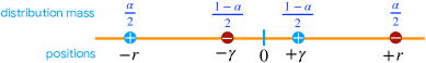
Fix $\alpha\in[0,1]$ and $\gamma\in(0,r)$. Consider the distribution $\mathscr{D}$ on the real line (dimension one) defined as follows: there is a probability mass of $\frac{\alpha}{2}$ at coordinate $(+r,-1)$, a probability mass of $\frac{\alpha}{2}$ at $(-r,+1)$, a probability mass of $\frac{1-\alpha}{2}$ at $(+\gamma,+1)$, and a probability mass of $\frac{1-\alpha}{2}$ at $(-\gamma,-1)$. Figure 3 illustrates this distribution. We first examine the expected hinge loss $\ell^{\mathsf{\,hinge}}(w)$ of an arbitrary linear classifier $w\in\mathbb{R}$ in dimension one:

$$\ell^{\mathsf{\,hinge}}(w) =\frac{\alpha}{2}\left[\max\left\{0,1+wr\right\}+\max\left\{0,1+wr\right\}\right]+\frac{1-\alpha}{2}\left[\max\left\{0,1-w\gamma\right\}+\max\left\{0,1-w\gamma\right\}\right]$$

$$=\alpha\max\left\{0,1+wr\right\}+(1-\alpha)\max\left\{0,1-w\gamma\right\}.$$

Thus, distinguishing cases based on the value of scalar $w$, we can write:

$$\ell^{\mathsf{\,hinge}}(w) =\begin{cases}\alpha(1+wr)+(1-\alpha)(1-w\gamma)&\text{if }w\in\left[0,\frac{1}{\gamma}\right]\\ \alpha(1+wr)&\text{if }w\geq\frac{1}{\gamma}\\ \alpha(1+wr)+(1-\alpha)(1-w\gamma)&\text{if }w\in\left[-\frac{1}{r},0\right]\\ (1-\alpha)(1-w\gamma)&\text{if }w\leq-\frac{1}{r}.\end{cases}$$

$$=\begin{cases}w(\alpha r-(1-\alpha)\gamma)+1&\text{if }w\in\left[0,\frac{1}{\gamma}\right]\\ \alpha(1+wr)&\text{if }w\geq\frac{1}{\gamma}\\ w(\alpha r-(1-\alpha)\gamma)+1&\text{if }w\in\left[-\frac{1}{r},0\right]\\ (1-\alpha)(1-w\gamma)&\text{if }w\leq-\frac{1}{r}.\end{cases}$$

To simplify the discussion, we will set $r=1$ and $\alpha=\frac{\gamma}{2}$, with $\gamma\ll 1$. This, implies $(\alpha r-(1-\alpha)\gamma)=\alpha(-1+2\alpha)<0$. As a result of this negative sign, the best solution for the first two cases above is $w=\frac{1}{\gamma}$, $w=0$ in the third case, and $w=-\frac{1}{r}$ in the last case. The loss achieved in the two latter cases is $1$ and $(1-\alpha)(1+\frac{\gamma}{r})$, both larger than the loss $\alpha\big{(}1+\frac{r}{\gamma}\big{)}$ obtained in the first two cases. In view of that, the overall minimizer of $\ell^{\mathsf{\,hinge}}(w)$ is given by $w^{*}=\frac{1}{\gamma}$, with $\ell^{\mathsf{\,hinge}}(w^{*})=\frac{1}{2}(1+\gamma)$. Note that the zero-one loss of $w^{*}$ is $\ell(w^{*})=\alpha=\frac{\gamma}{2}$.

Thus, for this example, the norm of the hinge-loss minimizer is arbitrary large: $\|w^{*}\|=\frac{1}{\gamma}\gg 1$. In particular, for a sample size $m$, we could choose $\gamma<\frac{1}{m}$, leading to $\|w^{*}\|>m$. Note that, here, any other positive classifier, $w>0$, achieves the same zero-one loss as $w^{*}$. For example, $w=1$ achieves the same performance as $w^{*}$ with a more favorable norm.

Our analysis was presented for the population hinge loss but a similar result holds for the empirical hinge loss.

Figure 3: Simple example in dimension one for which the minimizer of the expected hinge loss $\operatorname*{\mathbb{E}}[\ell^{\mathsf{\,hinge}}(w)]$ is $w^{*}=\frac{1}{\gamma}$ and thus $\|w^{*}\|=\frac{1}{\gamma}\gg 1$ for $\gamma\ll 1$.

References

• [AC06] Nir Ailon and Bernard Chazelle. Approximate nearest neighbors and the fast Johnson-Lindenstrauss transform. In Proceedings of the thirty-eighth annual ACM symposium on Theory of computing, pages 557–563, 2006.
• [AFKT21] Hilal Asi, Vitaly Feldman, Tomer Koren, and Kunal Talwar. Private stochastic convex optimization: Optimal rates in l1 geometry. arXiv preprint arXiv:2103.01516, 2021.
• [AKK+20] Thomas D. Ahle, Michael Kapralov, Jakob Bæk Tejs Knudsen, Rasmus Pagh, Ameya Velingker, David P. Woodruff, and Amir Zandieh. Oblivious sketching of high-degree polynomial kernels. In Shuchi Chawla, editor, Proceedings of the 2020 ACM-SIAM Symposium on Discrete Algorithms, SODA 2020, Salt Lake City, UT, USA, January 5-8, 2020, pages 141–160. SIAM, 2020.
• [AL09] Nir Ailon and Edo Liberty. Fast dimension reduction using rademacher series on dual BCH codes. Discrete & Computational Geometry, 42(4):615–630, 2009.
• [ALMM19] Noga Alon, Roi Livni, Maryanthe Malliaris, and Shay Moran. Private PAC learning implies finite littlestone dimension. In Moses Charikar and Edith Cohen, editors, Proceedings of the 51st Annual ACM SIGACT Symposium on Theory of Computing, STOC 2019, Phoenix, AZ, USA, June 23-26, 2019, pages 852–860. ACM, 2019.
• [ANW14] Haim Avron, Huy L. Nguyen, and David P. Woodruff. Subspace embeddings for the polynomial kernel. In Zoubin Ghahramani, Max Welling, Corinna Cortes, Neil D. Lawrence, and Kilian Q. Weinberger, editors, Advances in Neural Information Processing Systems 27: Annual Conference on Neural Information Processing Systems 2014, December 8-13 2014, Montreal, Quebec, Canada, pages 2258–2266, 2014.
• [Bar98] Peter L Bartlett. The sample complexity of pattern classification with neural networks: the size of the weights is more important than the size of the network. IEEE transactions on Information Theory, 44(2):525–536, 1998.
• [BDMN05] Avrim Blum, Cynthia Dwork, Frank McSherry, and Kobbi Nissim. Practical privacy: the sulq framework. In Chen Li, editor, Proceedings of the Twenty-fourth ACM SIGACT-SIGMOD-SIGART Symposium on Principles of Database Systems, June 13-15, 2005, Baltimore, Maryland, USA, pages 128–138. ACM, 2005.
• [BFSV+21a] Robert Istvan Busa-Fekete, Umar Syed, Sergei Vassilvitskii, et al. On the pitfalls of label differential privacy. In NeurIPS 2021 Workshop LatinX in AI, 2021.
• [BFSV+21b] Robert Istvan Busa-Fekete, Umar Syed, Sergei Vassilvitskii, et al. Population level privacy leakage in binary classification wtih label noise. In NeurIPS 2021 Workshop Privacy in Machine Learning, 2021.
• [BFTT19] Raef Bassily, Vitaly Feldman, Kunal Talwar, and Abhradeep Thakurta. Private stochastic convex optimization with optimal rates. arXiv preprint arXiv:1908.09970, 2019.
• [BGM21] Raef Bassily, Cristóbal Guzmán, and Michael Menart. Differentially private stochastic optimization: New results in convex and non-convex settings. arXiv preprint arXiv:2107.05585. Appeared at NeurIPS 2021., 2021.
• [BGN21] Raef Bassily, Cristóbal Guzmán, and Anupama Nandi. Non-euclidean differentially private stochastic convex optimization. arXiv preprint arXiv:2103.01278, 2021.
• [BNSV15] Mark Bun, Kobbi Nissim, Uri Stemmer, and Salil P. Vadhan. Differentially private release and learning of threshold functions. In Venkatesan Guruswami, editor, IEEE 56th Annual Symposium on Foundations of Computer Science, FOCS 2015, Berkeley, CA, USA, 17-20 October, 2015, pages 634–649. IEEE Computer Society, 2015.
• [BST99] Peter Bartlett and John Shawe-Taylor. Generalization performance of support vector machines and other pattern classifiers. Advances in kernel methods: support vector learning, pages 43–54, 1999.
• [BST14] Raef Bassily, Adam D. Smith, and Abhradeep Thakurta. Private empirical risk minimization: Efficient algorithms and tight error bounds. In 55th IEEE Annual Symposium on Foundations of Computer Science, FOCS 2014, Philadelphia, PA, USA, October 18-21, 2014, pages 464–473. IEEE Computer Society, 2014.
• [CGM19] Corinna Cortes, Spencer Greenberg, and Mehryar Mohri. Relative deviation learning bounds and generalization with unbounded loss functions. Annals of Mathematics and Artificial Intelligence, 85(1):45–70, 2019.
• [CHS14] Kamalika Chaudhuri, Daniel J. Hsu, and Shuang Song. The large margin mechanism for differentially private maximization. In Zoubin Ghahramani, Max Welling, Corinna Cortes, Neil D. Lawrence, and Kilian Q. Weinberger, editors, Advances in Neural Information Processing Systems 27: Annual Conference on Neural Information Processing Systems 2014, December 8-13 2014, Montreal, Quebec, Canada, pages 1287–1295, 2014.
• [CMS11] Kamalika Chaudhuri, Claire Monteleoni, and Anand D. Sarwate. Differentially private empirical risk minimization. J. Mach. Learn. Res., 12:1069–1109, 2011.
• [CMTS21] Corinna Cortes, Mehryar Mohri, and Ananda Theertha Suresh. Relative deviation margin bounds. In International Conference on Machine Learning, pages 2122–2131. PMLR, 2021.
• [DMNS06] Cynthia Dwork, Frank McSherry, Kobbi Nissim, and Adam D. Smith. Calibrating noise to sensitivity in private data analysis. In Shai Halevi and Tal Rabin, editors, Theory of Cryptography, Third Theory of Cryptography Conference, TCC 2006, New York, NY, USA, March 4-7, 2006, Proceedings, volume 3876 of Lecture Notes in Computer Science, pages 265–284. Springer, 2006.
• [DR14] Cynthia Dwork and Aaron Roth. The algorithmic foundations of differential privacy. Found. Trends Theor. Comput. Sci., 9(3-4):211–407, 2014.
• [Dwo06] Cynthia Dwork. Differential privacy. In Michele Bugliesi, Bart Preneel, Vladimiro Sassone, and Ingo Wegener, editors, Automata, Languages and Programming, 33rd International Colloquium, ICALP 2006, Venice, Italy, July 10-14, 2006, Proceedings, Part II, volume 4052 of Lecture Notes in Computer Science, pages 1–12. Springer, 2006.
• [EMSV21] Hossein Esfandiari, Vahab Mirrokni, Umar Syed, and Sergei Vassilvitskii. Label differential privacy via clustering. arXiv preprint arXiv:2110.02159, 2021.
• [FKT20] Vitaly Feldman, Tomer Koren, and Kunal Talwar. Private stochastic convex optimization: optimal rates in linear time. In Konstantin Makarychev, Yury Makarychev, Madhur Tulsiani, Gautam Kamath, and Julia Chuzhoy, editors, Proccedings of the 52nd Annual ACM SIGACT Symposium on Theory of Computing, STOC 2020, Chicago, IL, USA, June 22-26, 2020, pages 439–449. ACM, 2020.
• [GGK+21] Badih Ghazi, Noah Golowich, Ravi Kumar, Pasin Manurangsi, and Chiyuan Zhang. On deep learning with label differential privacy. arXiv preprint arXiv:2102.06062, 2021.
• [JL84] William B Johnson and Joram Lindenstrauss. Extensions of lipschitz mappings into a hilbert space 26. Contemporary mathematics, 26:28, 1984.
• [JT13] Prateek Jain and Abhradeep Thakurta. Differentially private learning with kernels. In International conference on machine learning, pages 118–126. PMLR, 2013.
• [JT14] Prateek Jain and Abhradeep Thakurta. (near) dimension independent risk bounds for differentially private learning. In ICML, 2014.
• [KP02] Vladmir Koltchinskii and Dmitry Panchenko. Empirical margin distributions and bounding the generalization error of combined classifiers. Annals of Statistics, 30, 2002.
• [KW11] Felix Krahmer and Rachel Ward. New and improved Johnson–Lindenstrauss embeddings via the restricted isometry property. SIAM Journal on Mathematical Analysis, 43(3):1269–1281, 2011.
• [LN17] Kasper Green Larsen and Jelani Nelson. Optimality of the johnson-lindenstrauss lemma. In 2017 IEEE 58th Annual Symposium on Foundations of Computer Science (FOCS), pages 633–638. IEEE, 2017.
• [LNUZ20] Huy Le Nguyen, Jonathan Ullman, and Lydia Zakynthinou. Efficient private algorithms for learning large-margin halfspaces. In Algorithmic Learning Theory, pages 704–724. PMLR, 2020.
• [LSS13] Quoc V. Le, Tamás Sarlós, and Alexander J. Smola. Fastfood - computing Hilbert space expansions in loglinear time. In Proceedings of the 30th International Conference on Machine Learning, ICML 2013, Atlanta, GA, USA, 16-21 June 2013, volume 28 of JMLR Workshop and Conference Proceedings, pages 244–252. JMLR.org, 2013.
• [MRT18] Mehryar Mohri, Afshin Rostamizadeh, and Ameet Talwalkar. Foundations of machine learning. MIT press, 2018.
• [MT07] Frank McSherry and Kunal Talwar. Mechanism design via differential privacy. In 48th Annual IEEE Symposium on Foundations of Computer Science (FOCS’07), pages 94–103. IEEE, 2007.
• [Nel10] Jelani Nelson. Johnson–Lindenstrauss notes, 2010.
• [Nel11] Jelani Jelani Osei Nelson. Sketching and streaming high-dimensional vectors. PhD thesis, Massachusetts Institute of Technology, 2011.
• [Nel15] Jelani Nelson. Dimensionality reduction—notes 2, 2015.
• [PP13] Ninh Pham and Rasmus Pagh. Fast and scalable polynomial kernels via explicit feature maps. In Proceedings of the 19th ACM SIGKDD international conference on Knowledge discovery and data mining, pages 239–247, 2013.
• [RBHT09] Benjamin IP Rubinstein, Peter L Bartlett, Ling Huang, and Nina Taft. Learning in a large function space: Privacy-preserving mechanisms for svm learning. arXiv preprint arXiv:0911.5708, 2009.
• [RR07] Ali Rahimi and Benjamin Recht. Random features for large-scale kernel machines. In John C. Platt, Daphne Koller, Yoram Singer, and Sam T. Roweis, editors, Advances in Neural Information Processing Systems 20, Proceedings of the Twenty-First Annual Conference on Neural Information Processing Systems, Vancouver, British Columbia, Canada, December 3-6, 2007, pages 1177–1184. Curran Associates, Inc., 2007.
• [RR08] Ali Rahimi and Benjamin Recht. Weighted sums of random kitchen sinks: Replacing minimization with randomization in learning. Advances in neural information processing systems, 21, 2008.
• [RS16] Sofya Raskhodnikova and Adam Smith. Lipschitz extensions for node-private graph statistics and the generalized exponential mechanism. In 2016 IEEE 57th Annual Symposium on Foundations of Computer Science (FOCS), pages 495–504. IEEE, 2016.
• [Rud17] Walter Rudin. Fourier analysis on groups. Courier Dover Publications, 2017.
• [SFBL97] Robert E. Schapire, Yoav Freund, Peter Bartlett, and Wee Sun Lee. Boosting the margin: A new explanation for the effectiveness of voting methods. In ICML, pages 322–330, 1997.
• [SS02] Bernhard Schölkopf and Alex Smola. Learning with Kernels. MIT Press: Cambridge, MA, 2002.
• [SSTT21] Shuang Song, Thomas Steinke, Om Thakkar, and Abhradeep Thakurta. Evading the curse of dimensionality in unconstrained private glms. In Arindam Banerjee and Kenji Fukumizu, editors, Proceedings of The 24th International Conference on Artificial Intelligence and Statistics, volume 130 of Proceedings of Machine Learning Research, pages 2638–2646. PMLR, 13–15 Apr 2021.
• [STC04] John Shawe-Taylor and Nello Cristianini. Kernel Methods for Pattern Analysis. Cambridge Univ. Press, 2004.
• [SWYZ21] Zhao Song, David P. Woodruff, Zheng Yu, and Lichen Zhang. Fast sketching of polynomial kernels of polynomial degree. In Marina Meila and Tong Zhang, editors, Proceedings of the 38th International Conference on Machine Learning, ICML 2021, 18-24 July 2021, Virtual Event, volume 139 of Proceedings of Machine Learning Research, pages 9812–9823. PMLR, 2021.
• [YSMN21] Sen Yuan, Milan Shen, Ilya Mironov, and Anderson CA Nascimento. Practical, label private deep learning training based on secure multiparty computation and differential privacy. Cryptology ePrint Archive, 2021.