lpcde: Local Polynomial Conditional Density Estimation and Inference

Abstract

This paper discusses the R package lpcde, which stands for local polynomial conditional density estimation. It implements the kernel-based local polynomial smoothing methods introduced in Cattaneo, Chandak, Jansson, and Ma (2022) for statistical estimation and inference of conditional distributions, densities, and derivatives thereof. The package offers pointwise and integrated mean square error optimal bandwidth selection and associated point estimators, as well as uncertainty quantification based on robust bias correction both pointwise (e.g., confidence intervals) and uniformly (e.g., confidence bands) over evaluation points. The methods implemented are boundary adaptive whenever the data is compactly supported. We contrast the functionalities of lpcde with existing R packages, and showcase its main features using simulated data.

Introduction

Conditional cumulative distribution functions (CDFs), probability density functions (PDFs), and derivatives thereof, are important parameters of interest in statistics, econometrics, and other data science disciplines. In this article, we discuss the main methodological features of the R package lpcde for estimation of and inference on conditional CDFs, PDFs, and derivatives thereof, employing the kernel-based local polynomial smoothing approach introduced in Cattaneo, Chandak, Jansson, and Ma (2022, CCJM hereafter).

Wand and Jones (1995), Fan and Gijbels (1996), Simonoff (2012) and Scott (2015) give textbook introductions to kernel-based density and local polynomial estimation and inference methods. The core idea underlying the estimator introduced in CCJM is to use kernel-based local polynomial smoothing methods to construct an automatically boundary adaptive estimator for CDFs, PDFs, and derivatives thereof. The estimation approach consists of two steps. The first step estimates the conditional distribution function using standard local polynomial regression methods, and the second step applies local polynomial smoothing to the (non-smooth) local polynomial conditional CDF estimate from the first step to obtain a smooth estimate of the CDF, PDF, and derivatives thereof.

For the case of PDF estimation, classical estimation approaches typically employ ratios of unconditional kernel density estimators, the derivative of kernel-based non-linear distribution function regression estimators, or local polynomial estimators based on some preliminary density-like approximation. See, for example, Fan, Yao, and Tong (1996), Hall, Wolff, and Yao (1999), De Gooijer and Zerom (2003), Hall, Racine, and Li (2004), and references therein. These approaches are not boundary adaptive unless specific modifications (e.g., boundary corrected kernels) are introduced. CCJM’s estimator is conceptually different and is boundary adaptive for a possibly unknown compact support of the data. Furthermore, the estimator has a simple closed form representation, which leads to easy and fast implementation. Unlike some other boundary adaptive procedures, it does not require pre-processing of data, and thus avoids the challenges of hyper-parameter tuning: only one bandwidth parameter needs to be selected for implementation.

Building on the theoretical and methodological work reported in CCJM, the package lpcde offers data-driven (pointwise and uniform) estimation and inference methods for conditional CDFs, PDFs, and derivatives thereof, which are automatically valid at interior, near-boundary, and boundary points on the support of both the variable of interest and the conditioning variables. For point estimation, the package offers mean squared error optimal bandwidth selection and associated point estimators. For inference, the package offers valid confidence intervals and confidence bands based on robust bias-correction techniques (Calonico, Cattaneo, and Farrell, 2018, 2022). Finally, these statistical procedures can be easily used for visualization and graphical presentation of smooth empirical CDFs, PDFs, and derivative thereof. We give an overview of the main methods implemented in the package below, along with a discussion of more specific implementation issues. We also showcase the performance of the package with simulated data.

The package lpcde includes two main functions.

• lpcde(): This function implements the estimator of interest over a grid of evaluation points on the support of the variable of interest and at a pre-specified conditioning value. The function takes three main inputs: data, a bandwidth, and polynomial orders. When the bandwidth is not specified by the user, the function employs the companion function lpbwcde() for automatic, data-driven bandwidth selection. When the polynomial orders are not specified by the user, the function employs the next odd polynomial order relative to the parameter of interest. For example, for CDF estimation, the polynomial orders are set to $\mathfrak{p}=\mathfrak{q}=1$, while for PDF estimation they are set to $\mathfrak{p}=2$ and $\mathfrak{q}=1$, where $\mathfrak{p}$ denotes the polynomial order for the variable of interest, and $\mathfrak{q}$ denotes the polynomial order for the conditioning variables. This function implements pointwise and uniform inference via robust bias-correction methods, employing the same grid of points used for point estimation.

• lpbwcde(): This function implements pointwise and integrated mean square error (IMSE) optimal bandwidth selection for the kernel-based local polynomial smoothing methods introduced in CCJM. The resulting bandwidth selection procedure leads to a IMSE-rate optimal point estimator whenever the difference of polynomial orders and derivatives order of interest is odd (see below for further details). This bandwidth choice is also valid, and in some cases optimal from a distributional approximation perspective, when coupled with robust bias-correction methods for statistical inference.

The methods coef(), confint(), vcov(), print(), plot() and summary() are supported for objects returned by the lpcde function, while the methods coef(), print() and summary() are supported for objects returned by the lpbwcde function. The plot() function builds on the ggplot2 (Wickham et al., 2021) package in R and can be used for illustrations of conditional CDFs, PDFs or higher order derivatives and their pointwise or uniform confidence bands for a given value of the conditioning variable(s).

The package lpcde contributes to a rather small set of R packages on CRAN for estimation and inference about conditional CDF, PDF, and derivatives thereof. More specifically, we identified two other packages that provide related methodology: hdrcde (Hyndman et al., 2021) and np (Racine and Hayfield, 2021). Table LABEL:table:rpkgs summarizes some of the main differences between those packages and lpcde. Additional information about the R package lpcde, including replication codes and datasets, can be found at https://nppackages.github.io/lpcde/.

Package Function	CDF / Derivative Estimation	Valid at Boundary	Standard Error	Valid Inference	Confidence Bands	Bandwidth Selection
hdrcde
cde	$\times$	$\times$	$\times$	$\times$	$\times$	✓
np
npcdens	$\times$	$\times$	✓	$\times$	$\times$	✓
lpcde
lpcde	✓	✓	✓	✓	✓	✓

Methodology

In this section, we give an overview of the methodology implemented in lpcde; technical details can be found in CCJM. We consider a collection of random samples $(Y_{1},\mathbf{X}_{1}^{\mathrm{T}}),\dots,(Y_{n},\mathbf{X}_{n}^{\mathrm{T}})$ from the continuously distributed random vector $(Y,\mathbf{X}^{\mathrm{T}})\in\mathcal{Y}\times\mathcal{X}$. We assume $\mathcal{Y}\subseteq\mathbb{R}$ is a $1$-dimensional and $\mathcal{X}\subseteq\mathbb{R}^{d}$ is a $d$-dimensional possibly, but not necessarily, compactly supported set. The goal is to estimate and conduct inference on the conditional CDF, PDF, and derivatives thereof, of $Y|\mathbf{X}$. Therefore, the parameter of interest is

$$F^{(\mu,\boldsymbol{\nu})}(y|\mathbf{x})=\frac{\partial^{\mu+|\boldsymbol{\nu}|}}{\partial y^{\mu}\partial\mathbf{x}^{\boldsymbol{\nu}}}F(y|\mathbf{x}),\qquad F(y|\mathbf{x})=\mathop{\operator@font IP\hskip 0.13pt}[Y\leq y|\mathbf{X}=\mathbf{x}],$$

where $\mu\in\mathbb{N}_{0}$ denotes the derivative order with respect to the variable of interest $Y$ and, employing multi-index notation, $\boldsymbol{\nu}\in\mathbb{N}^{d}_{0}$ denotes the multi-index for the corresponding derivatives of interest with respect to the conditioning variables $\mathbf{X}$. For example, $F(y|\mathbf{x})=F^{(0,\mathbf{0})}(y|\mathbf{x})$ corresponds to the conditional CDF of $Y|\mathbf{X}$, and $f(y|\mathbf{x})=F^{(1,\mathbf{0})}(y|\mathbf{x})$ corresponds to the conditional PDF of $Y|\mathbf{X}$, and $f^{(1,0)}(y|\mathbf{x})=F^{(2,\mathbf{0})}(y|\mathbf{x})$ corresponds to the derivative (with respect to $y$) of conditional PDF of $Y|\mathbf{X}$. To simplify the exposition, we abstract from derivative estimation with respect to the conditioning variables in $\mathbf{X}$, and therefore set $\boldsymbol{\nu}=\mathbf{0}$ for the rest of this article. Consequently, we define $F^{(\mu)}(y|\mathbf{x})=F^{(\mu,\mathbf{0})}(y|\mathbf{x})$ for $\mu\in\mathbb{N}_{0}$. See CCJM for theoretical and methodological results concerning $|\boldsymbol{\nu}|>0$, all of which are also implemented in the R package lpcde, thereby allowing for estimation of derivatives with respect to $\mathbf{X}$ of the conditional CDF of $Y|\mathbf{X}$.

General estimation idea

The construction of the conditional CDF, PDF and derivatives thereof involves two steps. First, the conditional distribution function $F(y|\mathbf{x})$ is estimated by standard local polynomial methods:

$$\widehat{F}_{\mathfrak{q}}(y|x)=\mathbf{e}_{0}^{\mathrm{T}}\widehat{\boldsymbol{\gamma}}_{\mathfrak{q}}(y|\mathbf{x}),\qquad\widehat{\boldsymbol{\gamma}}_{\mathfrak{q}}(y|\mathbf{x})=\operatorname*{argmin}_{\mathbf{c}\in\mathbb{R}^{\mathfrak{q}_{d}}}\sum_{i=1}^{n}\left(\mathds{1}(y_{i}\leq y)-\mathbf{q}(\mathbf{x}_{i}-\mathbf{x})^{\mathrm{T}}\mathbf{c}\right)^{2}L_{h}(\mathbf{x}_{i}-\mathbf{x}),$$

where $\mathbf{e}_{\ell}$ is the conformable $(\ell+1)$-th unit vector, $\mathbf{q}(\mathbf{u})$ denotes the $\mathfrak{q}_{d}$-dimensional vector collecting the ordered elements $\mathbf{u}^{\boldsymbol{\nu}}/\boldsymbol{\nu}!$ for $0\leq|\boldsymbol{\nu}|\leq\mathfrak{q}$, employing multi-index notation, $\mathfrak{q}_{d}=(d+\mathfrak{q})!/(\mathfrak{q}!d!)$, $\mathfrak{q}\in\mathbb{N}$, and $L_{h}(\mathbf{u})=K_{h}(u_{1})\cdots K_{h}(u_{d})$ is the product kernel for some kernel function $K(\cdot)$ and bandwidth parameter $h$. The resulting, standard $\mathfrak{q}$-th order local polynomial estimator $\widehat{F}_{\mathfrak{q}}(y|x)$ of $F(y|\mathbf{x})$ is not smooth as a function of $y$ and therefore cannot be used to construct an estimator of the conditional PDF and higher-order derivatives with respect to $y$.

Therefore, in a second step, a smoothed (with respect to $y$) estimator of the CDF and its derivatives is constructed also using local polynomial methods: for any $0\leq\mu\leq\mathfrak{p}$,

$$\widehat{F}^{(\mu)}_{\mathfrak{p},\mathfrak{q}}(y|\mathbf{x})=\mathbf{e}_{\mu}^{\mathrm{T}}\widehat{\boldsymbol{\beta}}_{\mathfrak{p},\mathfrak{q}}(y|\mathbf{x}),\qquad\widehat{\boldsymbol{\beta}}_{\mathfrak{p},\mathfrak{q}}(y|\mathbf{x})=\operatorname*{argmin}_{\mathbf{b}\in\mathbb{R}^{\mathfrak{p}+1}}\sum_{i=1}^{n}\left(\widehat{F}_{\mathfrak{q}}(y_{i}|\mathbf{x})-\mathbf{p}(y_{i}-y)^{\mathrm{T}}\mathbf{b}\right)^{2}K_{h}(y_{i}-y),$$

where $\mathbf{p}(u)$ denotes the vector collecting the ordered elements $u^{\mu}/\mu!$ for $0\leq\mu\leq\mathfrak{p}$. For a choice of derivative $\mu$ with respect to $y$ (and a choice of of derivative $\boldsymbol{\nu}$ with respect of $\mathbf{x}$; here set to $\boldsymbol{\nu}=0$ only for simplicity), a choice of polynomial orders $(\mathfrak{p},\mathfrak{q})$, a choice of bandwidth $h$ and kernel function $K(\cdot)$, the function lpcde() implements the estimator $\widehat{F}^{(\mu)}_{\mathfrak{p},\mathfrak{q}}(y|\mathbf{x})$ over a grid of points on $\mathcal{Y}$ for a given conditioning evaluation point $\mathbf{x}$. By default, the function sets $\mu=1$ and $\boldsymbol{\nu}=0$ (conditional PDF), $\mathfrak{q}=1$ (local linear nonsmooth conditional CDF estimation), $\mathfrak{p}=2$ (local quadratic smooth conditional CDF estimation), and $K(\cdot)$ is to chosen to be the Epanechnikov kernel. Generally speaking, it is recommended to choose the local polynomial order such that $\mathfrak{p}-\mu$ and $\mathfrak{q}-|\boldsymbol{\nu}|$ are both odd. Although the second-order Epanechnikov kernel is implemented by default, the function lpcde() can also be implemented with second-order uniform and triangular kernels by setting the variable kernel_type appropriately. The choice of the kernel does not affect the orders of the bias and the variance. Last but not least, the choice of bandwidth $h$ is important: by default, whenever $h$ is not supplied by the user, the function lpcde() relies on the companion function lpbwcde(), which implements data-driven bandwidth selection based on the minimization of the (approximate) mean squared error of the estimator $\widehat{F}^{(\mu)}_{\mathfrak{p},\mathfrak{q}}(y|\mathbf{x})$.

In the remainder of this section we review some of the main statistical properties and inference techniques developed in CCJM, which are implemented in the package lpcde.

Point estimation and bandwidth selection

Once we have the closed form point estimator, we can derive the leading bias and variance of the estimator. The leading bias and variance for odd values of $\mathfrak{p}-\mu$ and $\mathfrak{q}-|\boldsymbol{\nu}|$ take the following form:

$$\text{Bias}\left[\widehat{F}^{(\mu)}_{\mathfrak{p},\mathfrak{q}}(y|\mathbf{x})\right]=h^{\mathfrak{q}+1}B^{(\mu)}_{\mathfrak{q}+1}(y,\mathbf{x})+h^{\mathfrak{p}+1-\mu}B^{(\mu)}_{\mathfrak{p}+1}(y,\mathbf{x}),$$ (1)

$$\text{Var}\left[\widehat{F}^{(\mu)}_{\mathfrak{p},\mathfrak{q}}(y|\mathbf{x})\right]=\frac{1}{nh^{d+2\mu+1}}V^{(\mu)}_{\mathfrak{p},\mathfrak{q}}(y,\mathbf{x}).$$ (2)

Note that the quantities on the right hand side above implicitly depend on the kernel function. It is straightforward to show that $V^{(\mu)}_{\mathfrak{p},\mathfrak{q}}(y,\mathbf{x}),B^{(\mu)}_{\mathfrak{q}+1}(y,\mathbf{x}),B^{(\mu)}_{\mathfrak{p}+1}(y,\mathbf{x})$ converge in probability to non-random, well-defined limits. Exact expressions and technical details for other cases can be found in the supplemental appendix of CCJM.

Equations 1 and 2 are valid for all evaluation points on the support of the data. As a result, the pointwise mean squared error (MSE) optimal bandwidth can be expressed as

$$h_{\mathfrak{p},\mathfrak{q}}^{\text{MSE}}(y,\mathbf{x})=\operatorname*{argmin}_{h>0}\text{MSE}\left[\widehat{F}^{(\mu)}_{\mathfrak{p},\mathfrak{q}}(y|\mathbf{x})\right]=\operatorname*{argmin}_{h>0}\left[\text{Var}\left[\widehat{F}^{(\mu)}_{\mathfrak{p},\mathfrak{q}}(y|\mathbf{x})\right]+\text{Bias}\left[\widehat{F}^{(\mu)}_{\mathfrak{p},\mathfrak{q}}(y|\mathbf{x})\right]^{2}\right].$$

Under standard regularity conditions, $h^{\text{MSE}}(y,\mathbf{x})$ is MSE-optimal if $\mathfrak{p}-\mu$ and $\mathfrak{q}-|\boldsymbol{\nu}|$ are odd. Precise closed-form expressions for the MSE- optimal bandwidth can be found in the supplemental appendix of CCJM. In practice, the MSE-optimal bandwidth is estimated by computing plug-in estimates of the quantities in Equations 1 and 2, given some initial bandwidth choice, and then solving the following optimization problem

$$\widehat{h}_{\mathfrak{p},\mathfrak{q}}^{\text{MSE}}(y,\mathbf{x})=\operatorname*{argmin}_{h>0}\left[\widehat{\text{Var}}\left[\widehat{F}^{(\mu)}_{\mathfrak{p},\mathfrak{q}}(y|\mathbf{x})\right]+\widehat{\text{Bias}}\left[\widehat{F}^{(\mu)}_{\mathfrak{p},\mathfrak{q}}(y|\mathbf{x})\right]^{2}\right].$$

The IMSE-optimal bandwidth is estimated similarly, with the main difference being that a set of grid points on the support of $\mathcal{Y}$ is used to approximate the integral. Detailed expressions are given in the supplemental appendix. The number of grid points or specific locations of grid points can be specified by the user as an input to both the lpbwcde() and lpcde() functions. Bandwidth selection is implemented through the lpbwcde() function.

The variance-covariance estimator implemented in the package differs from the covariance estimator presented in CCJM. Rather than using the standard plug-in covariance estimator, which is slow to run in practice, the covariance estimator used in lpcde relies on the fact that the closed-form of the estimator can be written as a V-statistic to which the Hoeffding decomposition can be applied. The covariance expression decomposes to a sum of two independent functions that depend on the evaluation points and a small subset of the data in the neighborhood of the evaluation points. The expression is simple to write down and significantly faster to compute than the plug-in estimator in CCJM. This V-statistic covariance estimator is asymptotically equivalent to the theoretical variance expression derived in CCJM. See SA-6.1 in the supplemental appendix of CCJM for details.

Distribution theory and robust bias-corrected inference

In order to conduct inference, we first construct a Wald-type test statistic that has the following distributional convergence

$$T_{\mathfrak{p},\mathfrak{q}}(y,\mathbf{x})=\frac{\widehat{F}^{(\mu)}_{\mathfrak{p},\mathfrak{q}}(y|\mathbf{x})-F^{(\mu)}_{\mathfrak{p},\mathfrak{q}}(y|\mathbf{x})}{\sqrt{\text{Var}\left[\widehat{F}^{(\mu)}_{\mathfrak{p},\mathfrak{q}}(y|\mathbf{x})\right]}}\rightsquigarrow\mathcal{N}(B,1),$$

where $\rightsquigarrow$ denotes weak convergence as $n\to\infty$ and $h\to 0$, $\mathcal{N}$ denotes the Gaussian distribution, and $B$ denotes the standardized asymptotic bias emerging whenever a “large” bandwidth is employed (e.g., when the MSE-optimal or IMSE-optimal bandwidth is used). See CCJM for details.

Standard confidence intervals with nominal $(1-\alpha)$ coverage takes the form:

$$\text{CI}(y,\mathbf{x})=\left[\widehat{F}^{(\mu)}_{\mathfrak{p},\mathfrak{q}}(y|\mathbf{x})\pm z_{1-\alpha/2}\sqrt{\widehat{V}_{\mathfrak{p},\mathfrak{q}}(y|\mathbf{x})}\right],$$

where $\widehat{V}_{\mathfrak{p},\mathfrak{q}}(y|\mathbf{x})=\widehat{\text{Var}}\left[\widehat{F}^{(\mu)}_{\mathfrak{p},\mathfrak{q}}(y|\mathbf{x})\right]$, and $z_{\alpha}$ is the $\alpha$-th quantile of the standard normal distribution. However, for “large” bandwidths, this confidence interval would be invalid due to the asymptotic bias. In practice, often undersmoothing is used to address the asymptotic bias present. However, Calonico, Cattaneo, and Farrell (2018, 2022) show that undersmoothing is sub-optimal under the standard assumptions of the model. Instead, they propose a robust bias-correction (RBC) technique that has better higher-order approximations and asymptotically correct coverage probabilities. RBC requires bias-correction of the point estimator and then adjusting the variance estimate appropriately to construct a bias-corrected Wald-type statistic.

For our estimator, we first correct for the first-order bias by using a point estimator that is generated by increasing the polynomial order for both variables, $y$ and $\mathbf{x}$. To be specific, we use $\widehat{F}^{(\mu)}_{\mathfrak{p}+1,\mathfrak{q}+1}(y|\mathbf{x};h^{\text{MSE}}_{\mathfrak{p},\mathfrak{q}})$ in place of $\widehat{F}^{(\mu)}_{p,q}(y|\mathbf{x};h^{\text{MSE}}_{p,q})$. Note that the bandwidth used is optimal for the point estimate with the lower order polynomials. The asymptotically valid confidence intervals now take the form

$$\text{CI}^{\text{RBC}}(y,\mathbf{x})=\left[\widehat{F}^{(\mu)}_{\text{RBC}}(y|\mathbf{x})\pm z_{1-\alpha/2}\sqrt{\widehat{\text{Var}}\left[\widehat{F}^{(\mu)}_{\text{RBC}}(y|\mathbf{x})\right]}\right],$$

where $\widehat{F}^{(\mu)}_{\text{RBC}}(y|\mathbf{x})\equiv\widehat{F}^{(\mu)}_{\mathfrak{p}+1,\mathfrak{q}+1}(y|\mathbf{x})=\widehat{F}^{(\mu)}_{\mathfrak{p},\mathfrak{q}}(y|\mathbf{x})-\widehat{\text{Bias}}\left[\widehat{F}^{(\mu)}_{\mathfrak{p},\mathfrak{q}}(y|\mathbf{x})\right]$.

Additionally, uniform confidence bands can be constructed as

$$\text{CB}^{\text{RBC}}(\mathcal{M})=\left\{\left[\widehat{F}^{(\mu)}_{\text{RBC}}(y|\mathbf{x})\pm z_{\mathcal{M},1-\alpha/2}\sqrt{\widehat{\text{Var}}\left[\widehat{F}^{(\mu)}_{\text{RBC}}(y|\mathbf{x})\right]}\right],\quad y\in\mathcal{M}\right\},$$

where $\mathcal{M}$ is a collection of evaluation points on the support $\mathcal{Y}$ and $z_{\mathcal{M},\alpha}$ is the $\alpha$-quantile over the collection of evaluation points for a normal distribution centered at 0 and with the same variance-covariance matrix as the estimator. In practice, the critical value $z_{\mathcal{M},1-\alpha/2}$, is chosen by first simulating a Gaussian process on the grid $\mathcal{M}$ and then computing the upper $\alpha$ quantile of the supremum of the simulated process:

$$z_{\mathcal{M},\alpha} =\inf\left\{u\geq 0:\ \mathbb{P}\left[\left.\sup_{y\in\mathcal{M}}|\widehat{\mathcal{Z}}^{(\mu)}(y|\mathbf{x})|\leq u\right|\text{Data}\right]\geq 1-\alpha\right\},$$

where $\widehat{Z}^{(\mu)}(y|\mathbf{x})\sim\mathcal{N}\left(0,\widehat{\text{Cov}}\left[\widehat{F}^{(\mu)}_{\text{RBC}}(y|\mathbf{x})\right]\right)$. Note that the confidence band depends on the entire collection of evaluation points. See CCJM (and its supplemental) for technical details and regularity conditions.

Note that the RBC method leads to confidence intervals/bands that are not centered at the density point estimates since different order polynomials are used for the point estimates and for inference. Thus, it may happen that the point estimates is outside of the RBC confidence intervals/bands if the underlying distribution has high curvature at some evaluation point(s). One solution in this case is to increase the polynomial orders $\mathfrak{p}$ and $\mathfrak{q}$, or to use a smaller-than-optimal bandwidth.

Implementation

In this section we illustrate some of the main features of the package with simulated data. We consider a bi-variate jointly normal data generating process with mean $0$ and variance $1$.

Figure 1 illustrates the performance of the package for generating point estimates produced by lpcde() for the conditional (i) CDF (see Figures 1(a) and 1(b)), (ii) PDF (see Figures 1(c) and 1(d)), and (iii) first derivative (see Figures 1(e) and 1(f)) with both standard and robust bias-corrected confidence bands generated by the function lpcde(). The true functions are plotted in red for comparison.

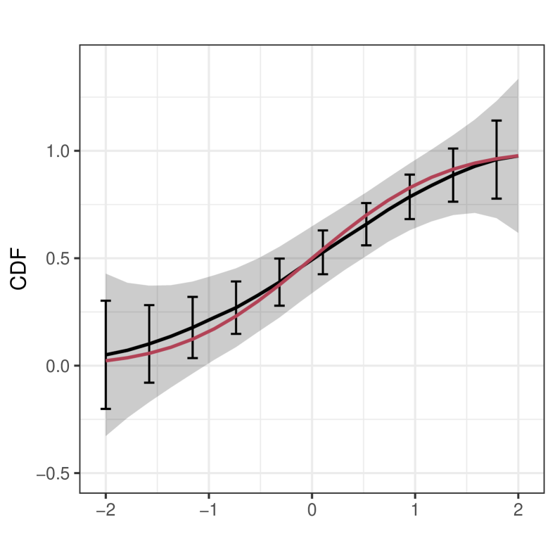
(a) standard CDF estimate.

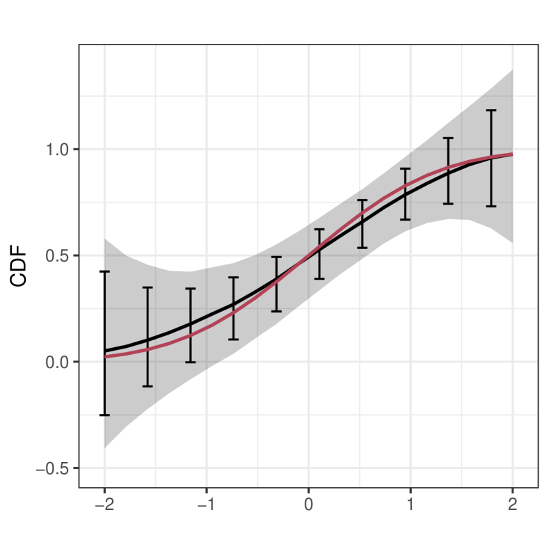
(b) RBC CDF estimate.

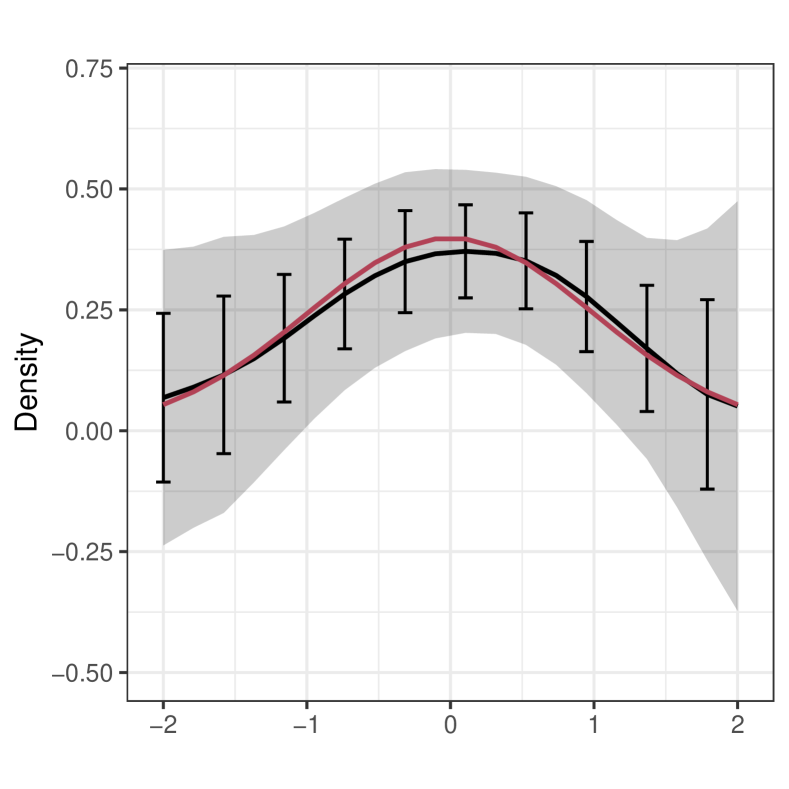
(c) standard PDF estimate.

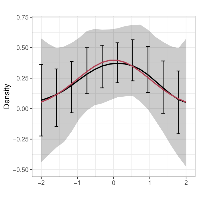
(d) RBC PDF estimate.

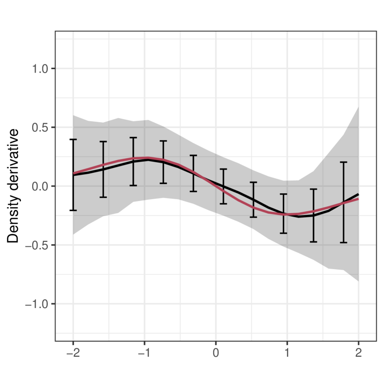
(e) standard first derivative estimate.

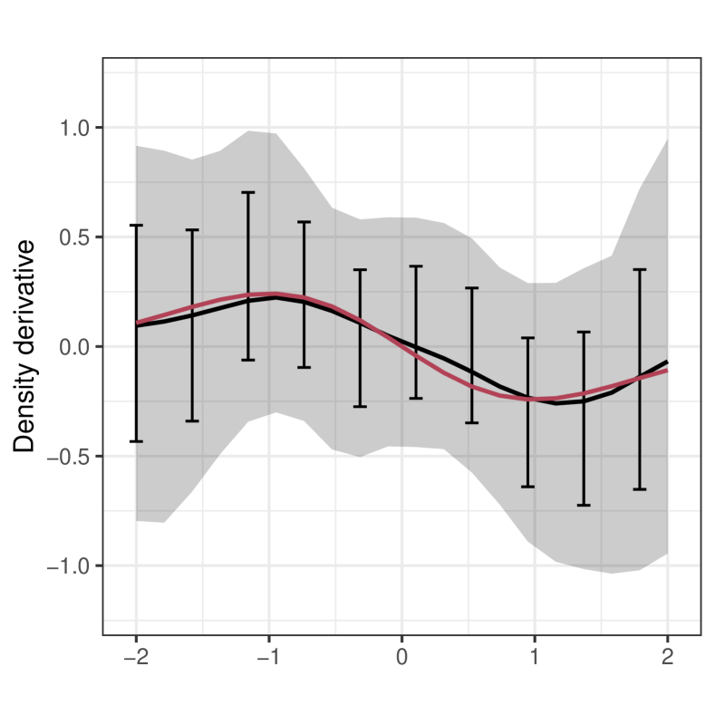
(f) RBC first derivative estimate.

Figure 1: Point estimate with 95% pointwise confidence intervals and uniform confidence bands. From Top to Bottom: CDF estimate, PDF estimate and first derivative estimate. From Left to Right: standard confidence interval/bands, robust bias-corrected confidence intervals/bands.

Density estimation with lpcde

The function lpcde() provides information on point estimates, standard errors and confidence interval or bands for a given value of $\mathbf{x}$ over a range of grid points for $y$. If the grid points are not provided by the user, the function chooses nineteen quantile-spaced grid points over the implied support of the data and, if no bandwidth is provided, computes the rule-of-thumb MSE bandwidth at each point.

The following example estimates the conditional density at $\mathbf{x}=0$, with a fixed bandwidth of $0.5$, using the default local polynomial approximation $\mathfrak{p}=2,\ \mathfrak{q}=1$. RBC confidence intervals over the grid are also computed, in this case using the default polynomial orders $\mathfrak{p}=3,\ \mathfrak{q}=2$.

    > set.seed(42)    > n = 1000    > x_data = as.matrix(stats::rnorm(n, mean = 0, sd = 1))    > y_data = as.matrix(stats::rnorm(n, mean = 0, sd = 1))    > y_grid = stats::quantile(y_data, seq(from=0.1, to=0.9, by=0.1))    > model1 = lpcde(y_data=y_data, x_data=x_data, y_grid=y_grid, x=0, bw = 0.5)    > summary(model1)

The function returns an object of type lpcde. Standard R methods, coef(), confint(), vcov(), print(), plot() and summary(), can be used on objects of type lpcde to understand the output.

For example, the first part of the summary output provides basic information about some of the options specified to the function. The second part provides relevant information for each point estimate generated in a table with $7$ columns, (i) grid evaluation points, (ii) bandwidth used at each point, (iii) effective number of data points used to generate the point estimate, (iv) point estimate, (v) standard error, (vi) lower $(1-\alpha)$-confidence interval, and, (vii) upper $(1-\alpha)$-confidence interval.

Call: lpcdeSample size                                           1000Polynomial order for Y point estimation      (p=)     2Polynomial order for X point estimation      (q=)     1Density function estimated                   (mu=)    1Order of derivative estimated for covariates (nu=)    0Kernel function                                       epanechnikovBandwidth method=============================================================================                                     Point      Std.       Robust B.C.Index     Grid      B.W.   Eff.n      Est.     Error      [ 95% C.I. ]=============================================================================1      -1.2512    0.5000      75    0.1656    0.0347    -0.0642 ,  0.36632      -0.8452    0.5000     108    0.3250    0.0277     0.1771 ,  0.47843      -0.5287    0.5000     142    0.3357    0.0188     0.1704 ,  0.45764      -0.2550    0.5000     139    0.3961    0.0211     0.3437 ,  0.62495      -0.0106    0.5000     146    0.3958    0.0219     0.2482 ,  0.5128-----------------------------------------------------------------------------6       0.2397    0.5000     150    0.3406    0.0181     0.1274 ,  0.35367       0.5039    0.5000     134    0.3572    0.0224     0.2355 ,  0.49938       0.8026    0.5000     111    0.3496    0.0313     0.2937 ,  0.64929       1.2896    0.5000      70    0.1651    0.0322    -0.1154 ,  0.3189=============================================================================

Plotting

The plot() function uses the ggplot2 package with objects of type lpcde to produce illustrations of point estimates and confidence intervals and/or bands. A simple plot of the conditional PDF with 95% confidence intervals can be generated by running the following code.

    > model1 = lpcde(y_data=y_data, x_data=x_data, x=0, bw = "mse-rot")    > plot(model1) + theme(legend.position = "none") By default the plot() function plots pointwise confidence intervals at $95\%$ level with the point estimates. Additional options for confidence levels, bands and RBC inference are detailed in the package manual. Editing other visuals of plots can be done by providing standard inputs to ggplot2 functions.

Bandwidth selection

lpbwcde() implements the rule-of-thumb MSE- and IMSE- bandwidth selection by implementing the formulae provided in previous sections.

By default lpbwcde() computes the rule-of-thumb MSE optimal bandwidth for the conditional PDF with locally quadratic polynomial in $y$ and locally linear polynomial in $\mathbf{x}$ and Epanechnikov kernel on nineteen grid points on the implied support of $\mathcal{Y}$ determined by the quantiles of the observed data. The output of this function is similar to that of lpcde() and provides basic information for the data and options specified. The summary of objects returned by this function additionally provides a table with three columns: (i) y_grid: values of the grid points for which the bandwidth is estimated, (ii) B.W.: the estimated bandwidth corresponding to each grid point, and (iii) Eff.n.: the number of effective data points at each evaluation point given the estimated bandwidth. An example of bandwidth selection, using the same data set as in previous example produces the following output.

    > y_grid = stats::quantile(y_data, seq(from=0.1, to=0.9, by=0.1))    > model2 = lpbwcde(y_data=y_data, x_data=x_data, x=0, y_grid = y_grid, bw_type = "mse-rot")    > summary(model2)

Call: lpbwcdeSample size                                           1000Polynomial order for Y point estimation      (p=)     2Polynomial order for X point estimation      (q=)     1Density function estimated                   (mu=)    1Order of derivative estimated for covariates (nu=)    0Kernel function                                       epanechnikovBandwidth method                                      mse-rot==================================Index     y_grid      B.W.   Eff.n==================================1      -1.2512    1.5671     5582      -0.8452    1.8298     7943      -0.5287    1.2936     6004      -0.2550    1.1646     5625      -0.0106    1.1336     567----------------------------------6       0.2397    1.1639     5447       0.5039    1.2844     5968       0.8026    1.7227     7519       1.2896    1.4860     503================================== The estimated bandwidth from this function can be used as bandwidth input to lpcde() directly by using the option of bwselect to specify bandwidth selection type instead of running lpbwcde() first.

Now we illustrate the effectiveness of our estimator with a Monte Carlo study. For the sake of simplicity, we set $d=1$ and assume that $\mathbf{x}$ and $y$ are simulated by a joint normal distribution with variance $2$ and covariance $-0.1$, truncated on $[-1,1]^{2}$. We simulate $1000$ data sets of $5000$ independent samples each. The results of this study are presented in Table 2. The point estimates are generated on $20$ evenly spaced grid points on $[0,1]$ for $y$.

We look at the performance of the estimator at three different derivative orders for the predictor variable, $y$, (i) the CDF, corresponding to $\mu=0$, (ii) the PDF, corresponding to $\mu=1$, and (iii) the first derivative of the conditional PDF with respect to $y$, corresponding to $\mu=2$, and three different conditional values of the covariate, $\mathbf{x}$: (a) interior, (b) near-boundary and (c) at-boundary. For each conditional value, we present the average rule-of-thumb bandwidth, average bias, standard deviation, pointwise and uniform $95\%$ coverage, and width of the confidence intervals/bands across the simulated datasets. We present these results for both the standard estimate (rows "WBC") which is generated with a quadratic polynomial ($\mathfrak{p}=2$) with respect to the variable $y$, and linear polynomial ($\mathfrak{q}=1$) with respect to the variable $\mathbf{x}$, as well as the robust bias-corrected estimates (rows "RBC") which uses cubic polynomial ($\mathfrak{p}=3$) for $y$ and quadratic polynomial ($\mathfrak{q}=2$) for $\mathbf{x}$.

					Coverage		Average Width
		$\widehat{h}_{\text{ROT}}$	bias	se	Pointwise	Uniform	Pointwise	Uniform
CDF ($\mu=0$)
$\mathbf{x}=0$	WBC	0.33	0.15	0.11	73.2	83.9	0.42	0.60
	RBC	0.33	0.15	0.13	85.8	93.5	0.51	0.73
$\mathbf{x}=0.8$	WBC	0.18	0.18	0.05	21.7	34.7	0.19	0.28
	RBC	0.18	0.18	0.14	70.8	91.7	0.54	0.82
$\mathbf{x}=1.0$	WBC	0.20	0.19	0.05	18.4	30.5	0.18	0.27
	RBC	0.20	0.19	0.14	68.1	90.8	0.53	0.80
PDF ($\mu=1$)
$\mathbf{x}=0$	WBC	0.38	0.09	0.03	60.4	78.9	0.11	0.23
	RBC	0.38	0.09	0.09	87.9	93.3	0.37	0.68
$\mathbf{x}=0.8$	WBC	0.35	0.10	0.04	73.0	84.6	0.22	0.40
	RBC	0.35	0.10	0.18	91.6	95.9	0.65	0.81
$\mathbf{x}=1.0$	WBC	0.38	0.10	0.06	55.8	77.0	0.24	0.45
	RBC	0.38	0.10	0.20	81.2	91.1	0.67	0.81
PDF Derivative ($\mu=2$)
$\mathbf{x}=0$	WBC	0.76	0.07	0.03	30.9	55.2	0.10	0.18
	RBC	0.76	0.07	0.12	67.1	92.2	0.48	0.87
$\mathbf{x}=0.8$	WBC	0.75	0.09	0.04	35.3	62.0	0.14	0.24
	RBC	0.75	0.09	0.16	74.9	91.4	0.64	1.17
$\mathbf{x}=1.0$	WBC	0.77	0.09	0.04	38.5	66.9	0.15	0.27
	RBC	0.77	0.09	0.18	78.8	92.9	0.69	1.25

Table 2: Table of average coverage for jointly normal data at three different conditional values. $\mathbf{x}=0$ is an interior point, $\mathbf{x}=0.8$ is a near-boundary point, $\mathbf{x}=1$ is at-boundary.
WBC: without bias-correction, RBC: robust bias-corrected.

Notice that robust bias-correction provides more accurate coverage, both pointwise and uniformly over the support across all derivative orders. We recommend, for accurate coverage probabilities, using uniform confidence bands with robust bias-corrected estimates.

We can also analyze the pointwise-in-$y$ performance of our estimator and inference methods. Table 3 presents the average pointwise results of 5000 simulated data sets. We consider three different evaluation points on the support of $y$ for the conditional PDF and three different values of the conditioning variable $\mathbf{x}$. The first four columns of the table present average pointwise MSE-optimal bandwidth used in estimation, effective sample size at each evaluation point, bias, and standard error. The last four columns are the average pointwise confidence interval coverage and width of the confidence interval for the standard estimate and inference method ("WBC") and robust bias-corrected estimate and inference ("RBC").

					Coverage		AW
Eval. point	$\widehat{h}_{\text{ROT}}$	eff.n	bias	se	WBC	RBC	WBC	RBC
$\mathbf{x}=0$
$y=0$	0.29	249	0.07	0.04	56.4	96.0	0.14	0.49
$y=0.8$	0.33	374	0.00	0.02	71.4	91.0	0.07	0.22
$y=1.0$	0.34	284	0.12	0.05	24.8	96.3	0.18	0.40
$\mathbf{x}=0.8$
$y=0$	0.24	140	0.07	0.07	77.4	98.6	0.20	0.68
$y=0.8$	0.30	297	0.00	0.02	78.0	94.1	0.07	0.24
$y=1.0$	0.36	256	0.13	0.05	54.0	91.6	0.18	0.37
$\mathbf{x}=1.0$
$y=0$	0.27	131	0.07	0.08	72.4	96.8	0.31	1.04
$y=0.8$	0.41	345	0.00	0.02	73.2	91.3	0.07	0.19
$y=1.0$	0.40	221	0.14	0.08	61.1	95.4	0.31	0.49

Table 3: Pointwise results
WBC: without bias-correction, RBC: robust bias-corrected.

We note that across all pointwise combinations, robust bias-corrected inference produces accurate coverage.

Finally, we test the rule-of-thumb MSE bandwidth selection by simulating point estimation and coverage at varying bandwidth values. We choose the range of bandwidth values to be between $0.5$ and $1.3$ times the average ROT bandwidth chosen by the lpbwcde() function. Table 4 presents the average bias, standard error, root mean-squared error, pointwise coverage rate and average width of confidence intervals for 5000 simulations at the interior point $y=0,\ \mathbf{x}=0$.

$\times\widehat{h}_{\text{MSE}}$	$\widehat{h}$	bias	se	rmse	WBC CR	RBC CR	WBC AW	RBC AW
0.5	0.15	0.07	0.31	0.34	100.0	100.0	1.23	4.14
0.6	0.18	0.07	0.18	0.20	99.7	100.0	0.69	2.37
0.7	0.20	0.07	0.11	0.14	97.7	100.0	0.43	1.46
0.8	0.23	0.07	0.07	0.11	87.8	99.5	0.28	0.96
0.9	0.26	0.07	0.05	0.09	74.8	98.6	0.20	0.67
1	0.29	0.07	0.04	0.08	56.4	96.0	0.14	0.49
1.1	0.32	0.06	0.03	0.07	39.6	89.8	0.11	0.37
1.2	0.35	0.07	0.02	0.07	25.5	81.4	0.08	0.28
1.3	0.38	0.06	0.02	0.07	16.0	72.6	0.06	0.22

Table 4: Bandwidth selection at interior point ($y=0,\mathbf{x}=0$).
WBC: without bias-correction, RBC: robust bias-corrected.

Conclusion

This article introduces the software package lpcde that computes local polynomial kernel based regression estimation and inference for conditional densities and higher-order derivatives. Additional information can be found at https://nppackages.github.io/lpcde/.

Matias D. Cattaneo
Department of Operations Research and Financial Engineering
Princeton University
United States of America
cattaneo@princeton.edu

Rajita Chandak
Department of Operations Research and Financial Engineering
Princeton University
United States of America
rchandak@princeton.edu

Michael Jansson
Department of Economics
University of California, Berkeley
United States of America
mjansson@econ.berkeley.edu

Xinwei Ma
Department of Economics
University of California, San Diego
United States of America
x1ma@ucsd.edu

References

- Calonico et al. (2018) S. Calonico, M. D. Cattaneo, and M. H. Farrell. On the effect of bias estimation on coverage accuracy in nonparametric inference. Journal of the American Statistical Association, 113(522):767–779, 2018.
- Calonico et al. (2022) S. Calonico, M. D. Cattaneo, and M. H. Farrell. Coverage error optimal confidence intervals for local polynomial regression. Bernoulli, 2022. forthcoming.
- Cattaneo et al. (2022) M. D. Cattaneo, R. Chandak, M. Jansson, and X. Ma. Local polynomial conditional density estimators. working paper, 2022.
- De Gooijer and Zerom (2003) J. G. De Gooijer and D. Zerom. On conditional density estimation. Statistica Neerlandica, 57(2):159–176, 2003.
- Fan and Gijbels (1996) J. Fan and I. Gijbels. Local Polynomial Modelling and Its Applications. Chapman & Hall/CRC, 1996.
- Fan et al. (1996) J. Fan, Q. Yao, and H. Tong. Estimation of conditional densities and sensitivity measures in nonlinear dynamical systems. Biometrika, 83(1):189–206, 1996.
- Hall et al. (1999) P. Hall, R. C. Wolff, and Q. Yao. Methods for estimating a conditional distribution function. Journal of the American Statistical association, 94(445):154–163, 1999.
- Hall et al. (2004) P. Hall, J. Racine, and Q. Li. Cross-validation and the estimation of conditional probability densities. Journal of the American Statistical Association, 99(468):1015–1026, 2004.
- Hyndman et al. (2021) R. Hyndman, J. Einbeck, and M. Wand. hdrcde: Highest Density Regions and Conditional Density Estimation, 2021. URL https://CRAN.R-project.org/package=hdrcde. R package version 3.4.
- Racine and Hayfield (2021) J. S. Racine and T. Hayfield. np: Nonparametric Kernel Smoothing Methods for Mixed Data Types, 2021. URL https://CRAN.R-project.org/package=np. R package version 0.60-11.
- Scott (2015) D. W. Scott. Multivariate Density Estimation: Theory, Practice, and Visualization. John Wiley & Sons, 2015.
- Simonoff (2012) J. S. Simonoff. Smoothing Methods in Statistics. Springer Science & Business Media, 2012.
- Wand and Jones (1995) M. Wand and M. Jones. Kernel Smoothing. Chapman & Hall/CRC, Florida, 1995.
- Wickham et al. (2021) H. Wickham, W. Chang, L. Henry, T. L. Pedersen, K. Takahashi, C. Wilke, K. Woo, H. Yutani, and D. Dunnington. ggplot2: Create Elegant Data Visualisations Using the Grammar of Graphics, 2021. URL https://CRAN.R-project.org/package=ggplot2. R package version 3.3.5.