In-vitro Major Arterial Cardiovascular Simulator to generate Benchmark Data Sets for in-silico Model Validation
Abstract
A deeper understanding of the influence of common cardiovascular diseases like stenosis, aneurysm or atherosclerosis on the circulatory mechanism is required, to establish new methods for early diagnosis. Different types of simulators were developed in the past to simulate healthy and pathological conditions of blood flow, often based on computational models, which allow to generate large data sets. However, since computational models often lack some aspects of real world data, hardware simulators are used to close this gap and generate data for model validation.
The aim of this study is the development and validation of a hardware simulator to generate benchmark data sets of healthy and pathological conditions. The in-vitro hardware simulator in this study includes the major 33 arteries and is driven by a ventricular assist device generating a parametrised input condition at the heart node. Physiologic flow conditions including heart rate, systolic/diastolic pressure, peripheral resistance and compliance are adjustable in a wide range. The pressure and flow waves at 17+1 different locations are measured by inverted fluid resistant pressure transducers and one ultrasound flow transducer supporting a detailed analysis of the measurement data. The pressure and flow waves show physiological conditions. Furthermore, the influence of stenoses degree and location on blood pressure and flow was investigated. The results indicate decreasing translesional pressure and flow with increasing degree of stenosis, as expected.
The benchmark data set is made available to the research community, with the purpose to validate and compare in-silico models of different type.
keywords:
Benchmark Datset , Cardiovascular Simulator , Validation of Computational Models , Stenosis1 Introduction
The prevalence of cardiovascular diseases is increasing worldwide [1]. Commonly atherosclerosis, stenosis and aneurysms are the major reason. Mortality is increasing with age and is also dependent on gender [2]. Early diagnoses of these diseases are desirable, consequently a deeper understanding of the influence of arterial diseases on the underlying system morphology and flow properties is necessary. Besides imaging techniques, which are often expensive and not available at primary physician level, there are currently no suitable mass screening methods to assess specific arterial properties at required accuracy. However, continuous quantities, like the Photoplethysmogramm (PPG) or pressure and flow, are obtained easily and contain information about the vascular structure, thus it would be desirable to infer the arterial properties from these signals [3].
Nowadays, on the other side, a variety of in-silico simulation models were developed to gain a deeper understanding of the circulatory mechanism by simulating healthy and pathologic conditions of cardiovascular blood pressure and flow by means of numerical models [4, 5, 6, 7, 8, 9, 10]. Given the patient-specific morphology and parameters, these computational simulation models are able to generate large data sets for the state variables of pressure and flow. In [11] for e.g., a virtual patient database was generated to study the influence of arterial diseases on the hemodynamics, by using a detailed arterial network from [12]. In [4], a confrontation of aorta (CoA) was simulated and has been successfully used to setup and identify patient-specific models and to reconstruct pre- and post-treatment scenarios characterized by available routine clinical data sets. The authors state that, for accurate remodelling of clinical situations, data acquirement in the clinic has to become more reliable to keep uncertainties small. Furthermore, due to the simplified model complexity (e.g. dimension reduction, shape optimisation, linearisation, etc.) data sets of numerical simulations lack some aspects of the real world data of the corresponding cardiovascular system. Consequently, such models have not yet made their way to clinical routine, because validation is still problematic [13].
Hardware simulators try to close this gap by generating parametric data sets of pressure and flow for model validation. In the last decade different types of in-vitro hardware simulators of the cardiovascular system were developed, mainly to verify computational fluid dynamics models [14, 15], to understand specific fluid dynamical conditions [16], or to validate ventricular assist devices [17, 18, 19]. In [16], a life-sized mock circulatory loop of the human circulation was developed for fluid-mechanical studies using an extracorporeal life support system and two pneumatically driven vascular assist devices (VADs) representing the left and right ventricle. Furthermore, mock circulatory loops often include no detailed mapping of the arterial system for test and validation of ventricular assist devices [17]. However, in [14] waveform measurements in a silicone arterial tree are compared to numerical predictions of a visco-elastic 1-D model to test the accuracy of the non-linear 1-D equations of blood flow in large arteries.
However, none of the hardware simulation setups was used as a tool to generate data sets containing relevant information about specific diseases for diagnostic purposes. Thus, the aim of this study is the development and validation of a patient-specific cardiovascular simulator to generate parametrical data sets, facing benchmark problems that characterize for e.g. the influence of arterial stenosis within the cardiovascular system and make these data sets available to the research community. Therefore, a Major Arterial Cardiovascular Simulator (MACSim) was developed and extended over the past years, integrating patho-physiological information to improve the understanding and validity of computer simulation models for interpretation in a clinical setting.
Within this work, a arterial network of the 33 major arteries was realised, the corresponding vessel morphology and parameters are presented. Furthermore, a detailed description of the measurement setup and procedure, including the definition and explanation of the different measurement scenarios, is given.
The physiologic measurement scenarios in this work were defined to quantify the impact of arterial abnormalities (e.g. stenosis) on the pressure and flow waves within the circulatory system. The pathological conditions of stenosis with different degree and location were addressed. Generated data sets are designed for the validation of computational simulation models to enable a community wide comparable statement of their quality. Specific data sets could be generated on author request. Moreover, the calibration of the pressure and flow sensors was established with high accuracy to allow high grade model validation. Finally, the measurement results of the different measurement scenarios are presented and discussed.
2 Materials and Methods
2.1 Cardiovascular Simulator
The development process of the simulator was led by six main design criteria with the aim to establish a modular and flexible simulation environment that is able to produce large statistical data sets of specific diseases within highly reproducible flow conditions:
-
1.
Minimization of the pulse wave reflection with the condition to obtain realistic wave reflections from peripheral bifurcations and pathologies.
-
2.
Adjustable flow conditions to a wide range of physiological conditions like for e.g. heart rate, systolic pressure, compliance, peripheral resistances, etc.
-
3.
Measurement of pressure and flow at several different locations within the cardiovascular simulator.
-
4.
Improved laboratory conditions for a highly reproducible pressure and flow measurement on sample a accurate time basis.
-
5.
Parametric scripting of ventricular boundary conditions.
-
6.
Persistent data management in relational data base for post-processing.
The multivariate statistical data sets include relevant meta-information about the experiments and are stored to a MySQL database for further analysis. In the context of this study the data set is made available via Matlab files for simple community wide post-processing. MySQL data can be obtained on author request.
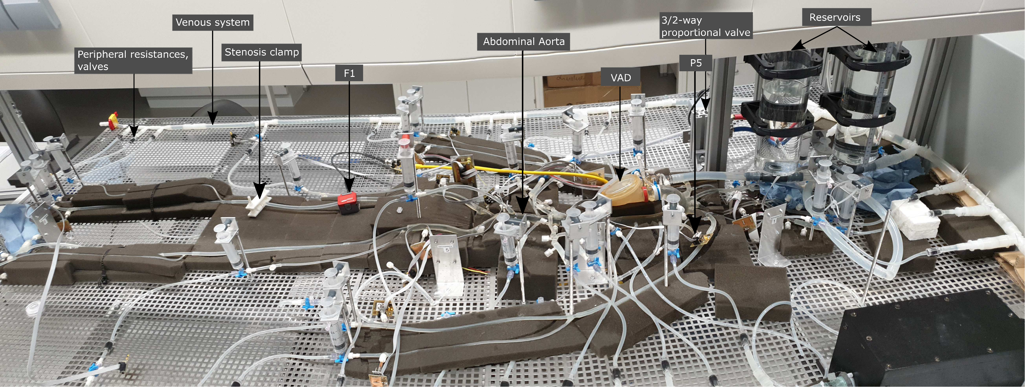
The experimental setup of the simulator consists of the following main components (see figure 1): arterial and venous system with valves and reservoirs, heart pump, compliance and peripheral resistance elements and pressure and flow sensors.
Arterial and Venous System
The structure of the cardiovascular simulator contains the major 33 arteries down to an inner diameter of 1,5 mm. This artificial arterial system is realised by a system of silicone tubes, which have similar characteristics such as inner and outer diameter, length and elasticity of the corresponding human arteries. The structural data for the arterial network was obtained from a real patient-specific MRI scan, followed by simplification and smoothing of the boundaries. Thereby, the individual parts of the arterial vascular system (aorta, art. carotis, art. subclavia, art. celiaca, art. iliaca and art. femoralis) were fabricated and assembled using injection molding. The other parts of the arterial system were made from standard silicon tubes due to the low vessel complexity and diameter. The whole vascular system is bedded on individually shaped PU-foam blocks, to ensure a proper anatomical tethering. In addition to the arterial vascular system, the simulator includes a venous return system and two reservoirs connecting the venous and arterial system (see figure 1 and 3).
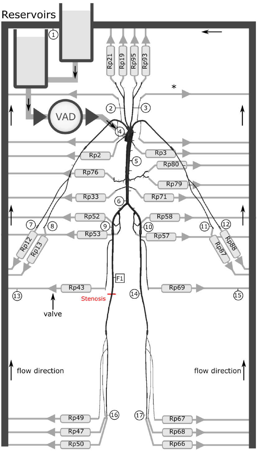
Since only measurements on the arterial vascular system are performed, a detailed mapping of the venous system was omitted and instead a simple feedback from the individual peripheral arteries to the reservoirs was realised. Both reservoirs are filled with of fluid, thus creating a hydrostatic pressure offset throughout the model cardiovascular system. The systems diastolic blood pressure, p̌, is set by a combination of the peripheral flow resistances, , and the level in the reservoirs.
The viscosity and density of the fluid in the simulator are adjusted to achieve physiological values for human blood by a water-glycerine mixture (approx. 60/40 weight %) , i.e. a resulting density of and a dynamic viscosity of at room temperature .
The node numbering of the arterial network refers to the computational simulation modelling environment SISCA [4]. In this software framework for multi-compartment lumped modelling each peripheral node number (see appendix figure 14) represents a flow resistance Rp in figure 1. The corresponding table 5 contains measurements and estimations for the vessel diameter d, length l, wall thickness h and elastic modulus E.
Heart Pump
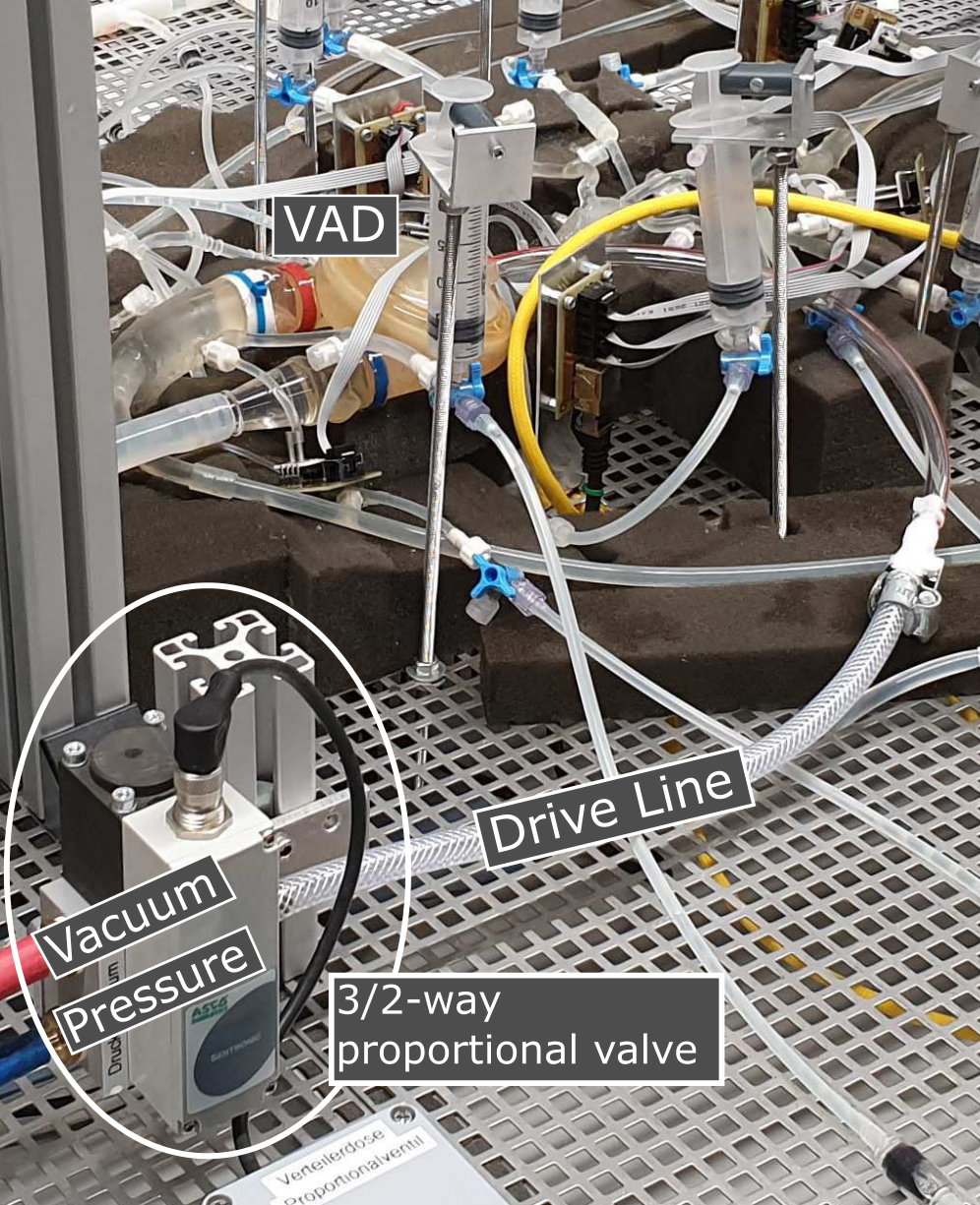
The simulator in-flow conditions at the heart node were realised by a pneumatically driven medical VAD (Ventricular Assist Device) diaphragm pump (Medos Stolberg, Germany) with maximum stroke volume of 80 ml, which provides a pulsatile fluid flow through the vascular system in a manner analogous to the left ventricle of the heart. The diaphragm pump is a medical device generally used as a external mechanical circulatory support system e.g. as bridge for heart transplant patients and therefore is suitable to create a pulsatile and heart-like pumping behaviour [20]. The diaphragm pump contains two heart valves and is controlled by a 3/2-way proportional valve (Series 614, Sentronic), which outputs the pressure for the drive line (see figure 2). The proportional valve applies the resulting pressure of a defined pressure curve by mixing an applied relative underpressure of and overpressure of . The vacuum pressure is generated by a pressure-controlled vacuum pump and stored in a recipient of 40 litre, to reduce long term drift during systole and realise long simulation times with stable pressure conditions.
During diastole the air side of the diaphragm pump is subjected to vacuum pressure reducing the air chamber volume, thus the membrane moves toward the air side and the ventricle is filled. The fluid is transported into the system by applying overpressure to push the medium out of the VAD through the arterial outlet.
Ftrapezoid
Peripheral Resistance and Compliance
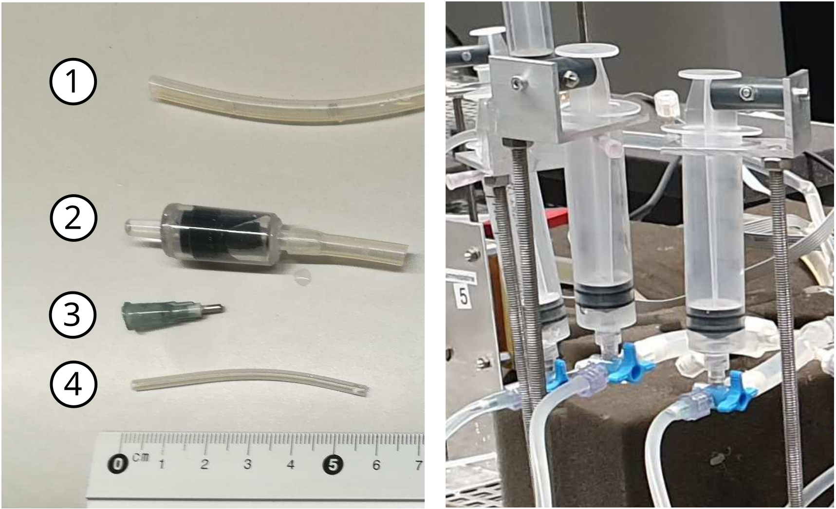
The physiological flow resistance of human arterioles and capillaries is modelled by additional small tubes inserted into the peripheral arteries, which open into the venous system (see figure 4). The peripheral resistance consists of the outer tube, a cannula with a small inner tube and a check valve. The length of the inner tubes was adjusted according to the physiological flow resistance of the arterial branch. Capillary flow resistance values were reproducibly generated downstream of each vessel end, the relative group values are found in table 1. Analogous to the venous valves in the human body, which prevent back flow in case of venous overpressure, for example, at the transition of the flow wave into the venous system, check valves were integrated to prevent back flow of fluid from the venous to the arterial system. The peripheral viscous flow resistance is defined as
| (1) |
where is the pressure difference and represents the volume flow.
The peripheral resistances of the boundary nodes were measured by the definition of regional groups like legs, arms, organs, head, etc. Table 1 shows the results in relation to the total peripheral resistance of the arterial system at the given viscosity (for detailed measurement description see appendix peripheral resistance measurement).
| Group | Corresponding elements | (%) |
|---|---|---|
| Head | 17,52 | |
| Coronar Art. | 5,57 | |
| Arm dextra | 14,94 | |
| Arm sinistra | 10,27 | |
| Organs | 23,12 | |
| Femoralis | 9,51 | |
| Leg dextra | 10,44 | |
| Leg sinistra | 8,63 |
Compensation and adjustments of the compliance were realised by syringes integrated vertically at the transition to the venous tube system (see figure 4). These are filled with a defined volume of air and thus create an artificial, additional distensibility of the respective vessels (all syringes were set to an air volume of , except at the peripheral nodes: and (see figure 1). The syringes can thus be considered as peripheral windkessel elements and have an impact on the total systems compliance. The compliance is defined as the extensibility of a artery and can be calculated by
| (2) |
where is the change in pressure for a prescribed change in volume . The total systems compliance was measured by adding a defined volume to the arterial system using a syringe connected via a luer-lock connector (for details see appendix compliance measurement figure 13).
Pressure and Flow Sensors
The pressure and flow was measured as a function of time, i.e. and at different locations in the system. Therefore, 17 pressure sensors (AMS 5812, 0050-D-I, inverted, fluid resistant) and a clamp-on medical grade ultrasonic-based flow sensor (SONOFLOW CO.55/060) were used to measure the flow velocity and the pressure in the system at predefined locations (see figure 1 and 3, label F1 and 1-17). Specific locations of the pressure and the flow sensors are shown in the schematic in figure 1. Prior measurement all sensors were calibrated, detailed measurement setup and calibration results are given in figure 12 in the appendix.
2.2 Measurement Setup and Procedure
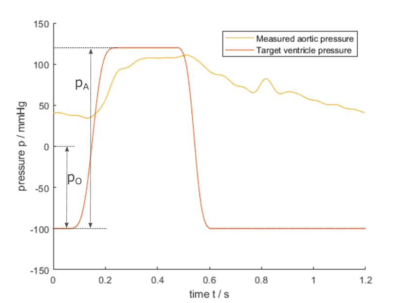
For each measurement scenario the pressure and flow was measured at 17 + 1 predefined locations respectively (see figure 1) . The input heart curve was chosen to be a trapezoidal curve (see figure 5), which was parametrised by an amplitude, offset, heart frequency and start and end of the ascending/descending slope (see equation 3). All measurements were acquired with a heart rate of and a maximum pressure amplitude of with an negative offset of . The trapezoidal curve was generated on a normalized time scale , where is the temporal period for the heart rate.
| (3) |
A linear raise was created between and followed by a plateau and a descent between and . The resulting curve was smoothed by Matlabs smoothdata function with a window length of 0,1 and rescaled along the time axis according to the applied heart rate (see figure 5).
The measurements were performed over a period of 60 seconds to guaranty steady state conditions and were acquired using a 16-bit data acquisition PCI-card (National Instruments, Austin, TX, USA) at sampling frequency of 1000 Hz per channel. The data acquisition software was entirely written in Matlab. The measurement data and meta-information was stored into a MySQL database for futher analysis.
2.3 Measurement Scenarios
The influence of stenoses on the pressure and flow in the cardiovascular system was investigated by simulating different measurement scenarios under healthy and pathological conditions. The healthy state serves as the reference without artificial stenoses. In the pathological setup an artificial stenosis in art. femoralis 20 cm downstream the knee (see figure 1) was chosen. The artery was squeezed reducing one axial dimension to a fraction between 3,3 % and 25 %, to obtain different degrees of stenosis (see table 2). This setting does not directly correspond to the clinical situation, where the stenosis cross-section is circular. In this study, the percent reduction of the artery is defined through the area change and the change in the diameter. The shape of the stenosed artery in squeezed form (see figure 6) is described by a rectangle with two attached half circles [21], then the cross-sectional area can be written as where is the width of the rectangle and the squeezed inner diameter as seen in figure 6. For negligible bending resistance in a thin walled tube, the circumference remains unchanged when squeezing the tube, in this case one can express the ratio as a function of the ratio , where is the cross-sectional area of the unsqueezed artery and is the initial inner diameter:
| (4) |
for .
| No. | ||
|---|---|---|
| I | 100 % | 100 % |
| II | 25 % | 37,5 % |
| III | 12,5 % | 23,4 % |
| IV | 3,3 % | 6,56 % |
All stenoses were established using a 3D-printed clamp (see figure 3 for the printed object and figure 6 for cross-section).

3 Results
The resulting data set is structured into four mat files, one per scenario. Each file contains 18 pressure signals and one flow signal, in total the data set contains 76 signals. The dataset and a detailed description is available at [22]. The following subsections describe the properties and results.
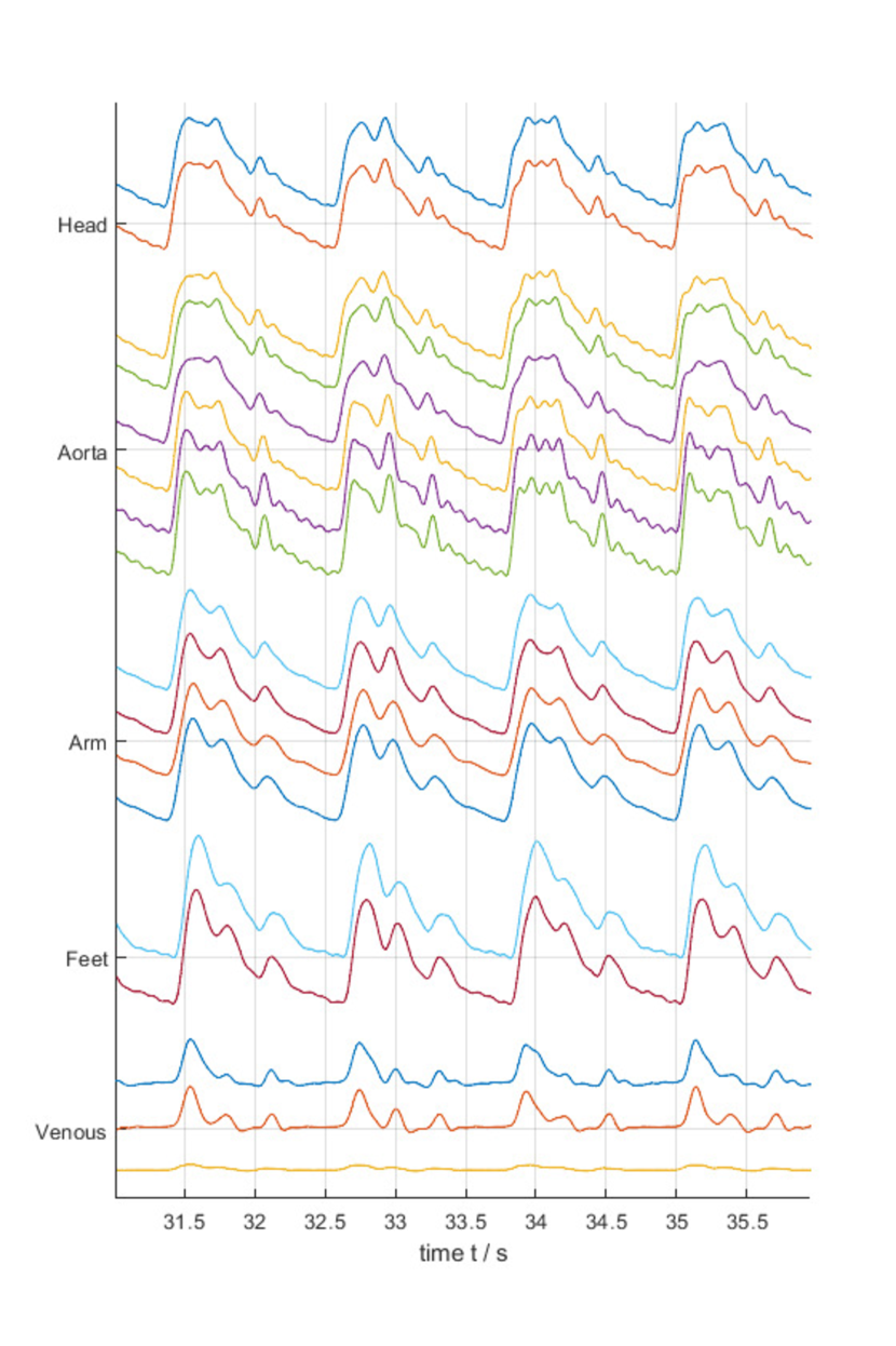
3.1 Pressure waves along the arterial network
Figure 7 shows the entire set of pressure curves along the arterial system under healthy conditions. Due to wave reflections of discontinuities the pressure waves clearly change their shape while propagating through the arterial system. As expected a short time delay between aortic and peripheral waves is observed (transit-time), which manifest, according to the wave velocity in the arterial network. The pressure amplitude increases in the peripheral vessels, which is in agreement with the pulse wave amplification observed in in-vivo measurements.
3.2 Scenario I - Healthy Conditions
In figure 8 the pressure wave at art. tibialis dextra under normal physiological conditions is shown. The result is similar to in-silico simulations and literature in terms of waveshape and specific wave features like the dicrotic notch and peripheral steeping.
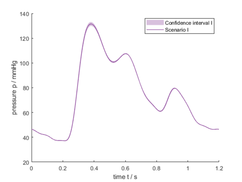
After the systolic rise to the peak pressure of , the blood pressure drops until the aortic valve closes, resulting into a dicrotic notch in the decaying pressure wave. This notch (incisure) is also found in human pressure waves. Subsequently, the pressure falls down to diastolic level of about , which is much lower than it would be physiologically.
The figures 8 to 10 contain confidence intervals calculated by the standard deviation of coherent averages, i.e. five averaging windows of the size of eight periods were used. The intervals represent the point-wise standard deviation and are used to show the temporal variation within the pressure waves. The confidence interval along the pressure waves is small, but increases at the systolic peak values and the discrotic notch. The mean value of the standard deviation of the systolic/diastolic peak values for pressure and flow for each scenario are given in table 3.
3.3 Scenarios II-VI - Pathological Conditions
The pathological conditions II-VI are based on a stenosis in the art. femoralis dextra with different stenosis degree (see table 2), corresponding the measurement result is given in figure 9 and 10.
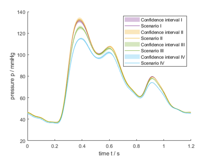
The pathological scenario II contains a stenosis in art. femoralis with a stenosis degree of . Due to the low degree of the stenosis there is no significant difference in the characteristics of the pressure wave, as expected the stenosis has low effect on the blood pressure: The pressure increases to a systolic peak value of and diastolic peak value of is observed.
The pathological scenario III contains a stenosis with a higher degree of , which causes a decrease of the pressure peak values of the pulse wave at the art. tibialis dextra (see figure 9). The systolic pressure peak decreases by 6 mmHg to an amplitude of , while the diastolic pressure remains constant at . Compared to the healthy setup, the shape of the pulse waves distal to the stenosis smoothes due to the reduction of the vessel’s effective diameter by the constriction. As expected the scenario IV has the lowest systolic pressure of all scenarios. In comparison to the reference scenario I the systolic pressure significantly decreases by 16 mmHg to a peak value of .
The mean pressure values for each scenario are given in table 3. With increasing stenosis degree the mean pressure decreases, but not that strong as the peak values . The difference of the mean pressure between scenario I and IV is only 4,3 mmHg, which can explained by the fact that although the systolic pressure decreases, the diastolic pressure remains at the same level for all scenarios.
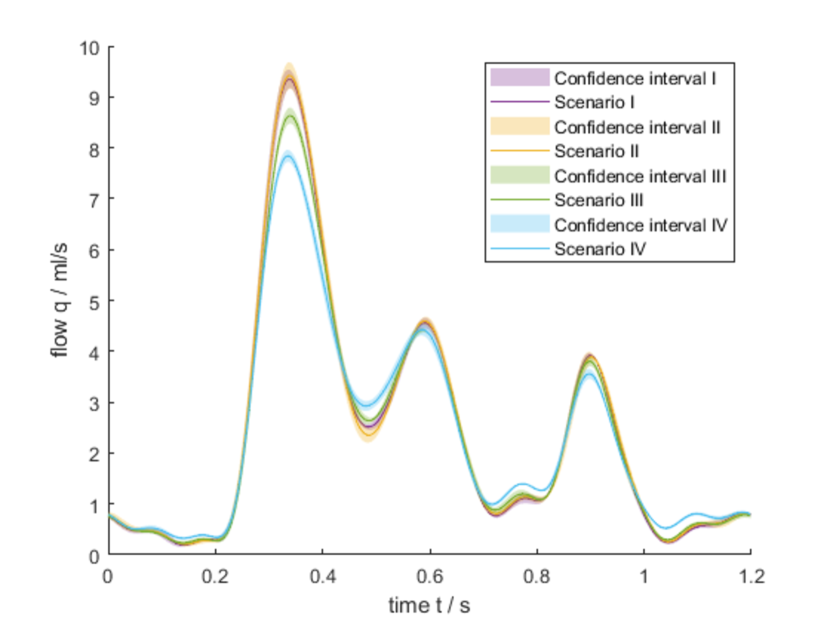
In figure 10 the flow waves at the art. profunda femoris dextra are shown for all measurement scenarios. The peak values of the flow velocity for the healthy state (scenario I) is , and for all pathological conditions reduced as expected , and . Consequently, the flow velocity within the diseased vessel decreases with an increasing degree of the stenosis. The mean flow values for each scenario are given in table 3. In contrast to the peak values the mean flow remains almost constant.
| No. | (mmHg) | (mmHg) | (mmHg) | (mmHg) | (ml/s) | (ml/s) | (ml/s) |
|---|---|---|---|---|---|---|---|
| I | 132,0 | 37,2 | 73,7 | 0,7 | 9,4 | 2,4 | 0,1 |
| II | 133,0 | 37,4 | 73,9 | 0,8 | 9,3 | 2,4 | 0,1 |
| III | 126,0 | 37,0 | 72,4 | 0,7 | 8,6 | 2,3 | 0,1 |
| IV | 115,8 | 36,2 | 69,4 | 0,6 | 7,8 | 2,3 | 0,1 |
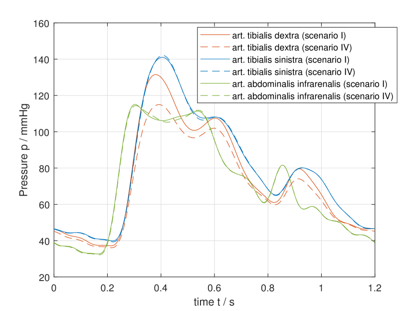
Finally, figure 11, shows the influence of the stenosis on different adjacent arteries like art. abdominalis infrarenalis and art. tibialis dextra and sinistra. In scenario I without stenosis , while in scenario IV . The pressure wave measured in the right foot decreases, while the pressure measured in the aorta and in the left foot remain visually unchanged.
4 Discussion
The purpose of this study was the development and validation of a patient-specific in-vitro hardware simulator to generate parametric data sets under healthy and pathological conditions for computational model validation.
In the past years, different hardware simulators were developed to investigate various theses, thus the three dimensional arterial structure differs in complexity, in the type of heart pump, in the number of sensors and in properties like compliance and peripheral resistances. In [16], the simulator drive consists of two pneumatically driven VADs representing the right and the left ventricle. In [23], a harvard pulsatile pump is used. Furthermore, both hardware simulators [16, 23] contain detailed arterial network covering 37 major arteries of the human body. Whereas hardware simulators with the aim to test and validate VADs, include an arterial network of low complexity and a simple functional drive.
The simulator in this work is pneumatically driven by one VAD to provide a pulsatile fluid flow through the vascular system. The arterial network contains a detailed arterial network with adjustable elements regarding heart rate, systolic/diastolic pressure, compliance and peripheral resistances. Furthermore, the simulator provides 17 pressure sensors at different locations and one flow sensor, which enables a detailed evaluation of the wave propagation. Due to material properties the total arterial compliance of the simulator is and therefore lower than in-vivo. The total peripheral resistance is . The low compliance evokes that the stiffness of arteries is higher than in-vivo, which indicates an atherosclerotic, high-blood-pressure patient. In contrast the arterial compliance in [16] was adjusted to and in [23] no peripheral compliances are included.
As shown in the results section, the pressure waves within the simulator contain similar properties as in-vivo measurements. The waveshape and specific wave features like the discrotic notch, peripheral steeping and translational pressure drop are observed. Furthermore, due to wave reflection at discontinuities and compliance variation of the vessels the shape of the pressure changes while propagating through the system.
Moreover, the influence of a stenosis and its degree on the pulse wave in the circulatory system was investigated. As expected, the results imply that for higher degree of stenosis the pressure after the diseased vessel decreases. The flow measurements show similar results (see figure 10): for higher degree of stenosis the flow decreases, as expected. These results are in good conformity to results provided by other hardware simulators [24, 14]. Furthermore, the influence of stenosis on different arteries were examined. Figure 11 shows that the stenosis at art. femoralis dextra has only an significant impact on the diseased vessel in the right leg, where the pressure decreases. Thereby, the pressure wave in the aorta and the left leg remain visually unchanged. The measurements under physiologic and pathological conditions confirm the validity of the in-vitro hardware simulator.
However, certain limitations concerning the results of this study could be addressed in future research. A first limitation concerns the low compliance of the arterial system as well as the peripheral resistances, which are too high. The compliance could be adjusted by a higher volume of the syringes within the system. To get more physiological peripheral resistances the impact of the different resistance elements like inner tubes and valves could be adjusted. A further potential limitation are the measured pressure waves, which are affected by noise in a broad frequency range. The reason for this are the vibrations of the systems components due to pumping process of the VAD. This could be fixed in future research by a more efficient embedding of the tube system with the PU-foam blocks. Moreover, the diastolic pressure of about 40 mmHg is too low in comparison with in-vivo measurements. The reason for this may be the low compliance and the high peripheral resistances within the system.
In conclusion, the present study has provided measurement data to the community, which hopefully provides support for the validation of computational models. In addition, the improvement of the pathological understanding will enable interpretation in a clinical setting through validation of computational models.
In terms of future research, it would be useful to extend the current findings by generating a data set with the hardware simulator developed, that can be used to develop and test algorithms for stenosis detection and localization on physical in-vitro data.
5 Conclusion
Within this study a in-vitro cardiovascular hardware simulator was developed and validated to gain a deeper understanding of blood pressure and flow under healthy and pathological conditions.
Physiological flow conditions are adjustable in a wide range by changing parameters like heart rate, systolic/diastolic pressure, compliance and peripheral resistances. The pressure and flow waves show similar wave form compared to in-vivo measurements. Moreover, the pressure and flow waves show the expected behaviour, in case of a stenosis of different location and degree.
This work provides measurement data containing healthy and pathological conditions like stenoses to the research community, to support the validation of computational models in near future.
Declaration of competing interest
All authors declare that there is no conflict of interest in this work.
References
- [1] F. G. R. Fowkes, D. Rudan, I. Rudan, V. Aboyans, J. O. Denenberg, M. M. McDermott, P. E. Norman, U. K. A. Sampson, L. J. Williams, G. A. Mensah, M. H. Criqui, Comparison of global estimates of prevalence and risk factors for peripheral artery disease in 2000 and 2010: a systematic review and analysis, The Lancet 382 (9901) (2013) 1329–1340. doi:10.1016/S0140-6736(13)61249-0.
- [2] E. B. Mathiesen, O. Joakimsen, K. H. Bønaa, Prevalence of and risk factors associated with carotid artery stenosis: the tromsø study, Cerebrovascular diseases (Basel, Switzerland) 12 (1) (2001) 44–51. doi:10.1159/000047680.
- [3] C. M. Quick, W. L. Young, A. Noordergraaf, Infinite number of solutions to the hemodynamic inverse problem, American Journal of Physiology-Heart and Circulatory Physiology 280 (4) (2001) H1472–9. doi:10.1152/ajpheart.2001.280.4.H1472.
- [4] R. Huttary, L. Goubergrits, C. Schütte, S. Bernhard, Simulation, identification and statistical variation in cardiovascular analysis (sisca) - a software framework for multi-compartment lumped modeling, Computers in Biology and Medicine 87 (2017) 104–123. doi:10.1016/j.compbiomed.2017.05.021.
- [5] R. Gul, S. Bernhard, Parametric uncertainty and global sensitivity analysis in a model of the carotid bifurcation: Identification and ranking of most sensitive model parameters, Mathematical biosciences 269 (2015) 104–116. doi:10.1016/j.mbs.2015.09.001.
- [6] A. Quarteroni, A. Veneziani, C. Vergara, Geometric multiscale modeling of the cardiovascular system, between theory and practice, Computer Methods in Applied Mechanics and Engineering 302 (2016) 193–252. doi:10.1016/j.cma.2016.01.007.
- [7] A. Quarteroni, S. Ragni, A. Veneziani, Coupling between lumped and distributed models for blood flow problems, Computing and Visualization in Science 4 (2) (2001) 111–124. doi:10.1007/s007910100063.
- [8] S. Zenker, J. Rubin, G. Clermont, From inverse problems in mathematical physiology to quantitative differential diagnoses, PLoS computational biology 3 (11) (2007) e204. doi:10.1371/journal.pcbi.0030204.
- [9] L. Garber, S. Khodaei, Z. Keshavarz-Motamed, The critical role of lumped parameter models in patient-specific cardiovascular simulations, Archives of Computational Methods in Engineering (2021). doi:10.1007/s11831-021-09685-5.
- [10] F. Ježek, T. Kulhánek, K. Kalecký, J. Kofránek, Lumped models of the cardiovascular system of various complexity, Biocybernetics and Biomedical Engineering 37 (4) (2017) 666–678. doi:10.1016/j.bbe.2017.08.001.
- [11] G. Jones, J. Parr, P. Nithiarasu, S. Pant, A physiologically realistic virtual patient database for the study of arterial haemodynamics, International Journal for Numerical Methods in Biomedical Engineering (2021) e3497doi:10.1002/cnm.3497.
- [12] E. Boileau, P. Nithiarasu, P. J. Blanco, L. O. Müller, F. E. Fossan, L. R. Hellevik, W. P. Donders, W. Huberts, M. Willemet, J. Alastruey, A benchmark study of numerical schemes for one-dimensional arterial blood flow modelling, International Journal for Numerical Methods in Biomedical Engineering 31 (10) (2015) e02732. doi:10.1002/cnm.2732.
- [13] I. E. Vignon-Clementel, D. Chapelle, A. I. Barakat, A. Bel-Brunon, P. Moireau, E. Vibert, Special issue of the vph2020 conference:virtual physiological human: When models, methods and experiments meet the clinic, Annals of biomedical engineering (2022). doi:10.1007/s10439-022-02943-y.
- [14] W. Jin, J. Alastruey, Arterial pulse wave propagation across stenoses and aneurysms: assessment of one-dimensional simulations against three-dimensional simulations and in vitro measurements, Journal of the Royal Society, Interface 18 (177) (2021) 20200881. doi:10.1098/rsif.2020.0881.
- [15] P. Korzeniowski, R. J. White, F. Bello, Vcsim3: a vr simulator for cardiovascular interventions, International journal of computer assisted radiology and surgery 13 (1) (2018) 135–149. doi:10.1007/s11548-017-1679-1.
- [16] J. Gehron, J. Zirbes, M. Bongert, S. Schäfer, M. Fiebich, G. Krombach, A. Böning, P. Grieshaber, Development and validation of a life-sized mock circulatory loop of the human circulation for fluid-mechanical studies, ASAIO journal (American Society for Artificial Internal Organs : 1992) 65 (8) (2019) 788–797. doi:10.1097/MAT.0000000000000880.
- [17] G. Ferrari, C. de Lazzari, M. Kozarski, F. Clemente, K. Górczynska, R. Mimmo, E. Monnanni, G. Tosti, M. Guaragno, A hybrid mock circulatory system: Testing a prototype under physiologic and pathological conditions, ASAIO Journal 48 (5) (2002) 487.
- [18] A. A. Pugovkin, S. V. Selishchev, D. V. Telyshev, Simulator for modeling the cardiovascular system for testing circulatory assist devices, Biomedical Engineering 49 (4) (2015) 213–216. doi:10.1007/s10527-015-9542-6.
- [19] A. A. Pugovkin, D. V. Telyshev, Automated pediatric cardiovascular simulator for left ventricular assist device evaluation, in: 2017 International Siberian Conference on Control and Communications (SIBCON), IEEE, 6/29/2017 - 6/30/2017, pp. 1–4. doi:10.1109/SIBCON.2017.7998543.
- [20] S. Thuaudet, The medos ventricular assist device system, Perfusion 15 (4) (2000) 337–343. doi:10.1177/026765910001500409.
- [21] S. Bernhard, S. Möhlenkamp, A. Tilgner, Transient integral boundary layer method to calculate the translesional pressure drop and the fractional flow reserve in myocardial bridges, Biomedical engineering online 5 (2006) 42. doi:10.1186/1475-925X-5-42.
- [22] S. Bernhard, M. Wisotzki, P. Schlett, B. Lindner, A. Mair, M. Oberhardt, In-vitro major arterial cardiovascular simulator: Benchmark data set for in-silico model validation. doi:10.5281/ZENODO.6415276.
- [23] K. S. Matthys, J. Alastruey, J. Peiró, A. W. Khir, P. Segers, P. R. Verdonck, K. H. Parker, S. J. Sherwin, Pulse wave propagation in a model human arterial network: assessment of 1-d numerical simulations against in vitro measurements, Journal of biomechanics 40 (15) (2007) 3476–3486. doi:10.1016/j.jbiomech.2007.05.027.
- [24] W. S. Hacham, A. W. Khir, The speed, reflection and intensity of waves propagating in flexible tubes with aneurysm and stenosis: Experimental investigation, Proceedings of the Institution of Mechanical Engineers. Part H, Journal of engineering in medicine 233 (10) (2019) 979–988. doi:10.1177/0954411919859994.
-
[25]
agbernhard.lse.thm.de /
sisca · gitlab (06.04.2022).
URL https://gitlab.com/agbernhard.lse.thm/sisca/
Appendix
Calibration Measurements
All pressure and flow sensors used in this study were calibrated to ensure valid measurement data.
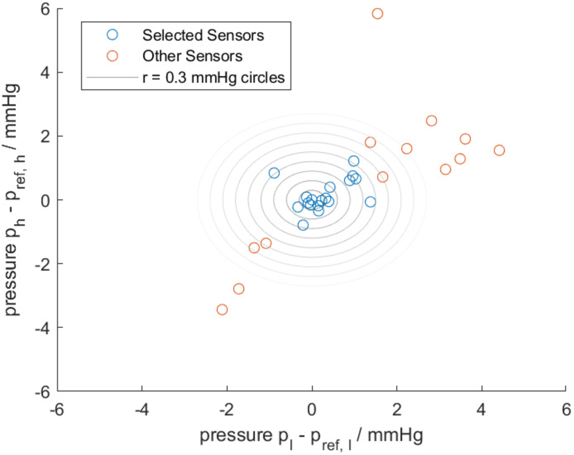
Calibration Pressure Sensors
The pressure sensors were calibrated through a two-point calibration measurement. Therefore, a bag filled with water was set to a defined hydrostatic pressure. This pressure corresponds to a water column of . Subsequently, the hydrostatic pressure was set to compared to the atmospheric pressure for the second point for the calibration measurement. In each calibration measurement a reference sensor, , was present to compare the measurement values. The results of the calibration measurement for each sensor is shown in figure 12. All sensors used lie within a maximum deviation of .
Calibration Flow Sensor
The flow sensor was calibrated through a two-point calibration measurement, where the volume difference between the steady state and running system was evaluated at location F1 (see figure 1). Volume integration was done by disconnection of reservoirs and determination of the fluid amount per time. Subsequently, the mean flow velocity and a correction factor of 4,8 were calculated.
Compliance
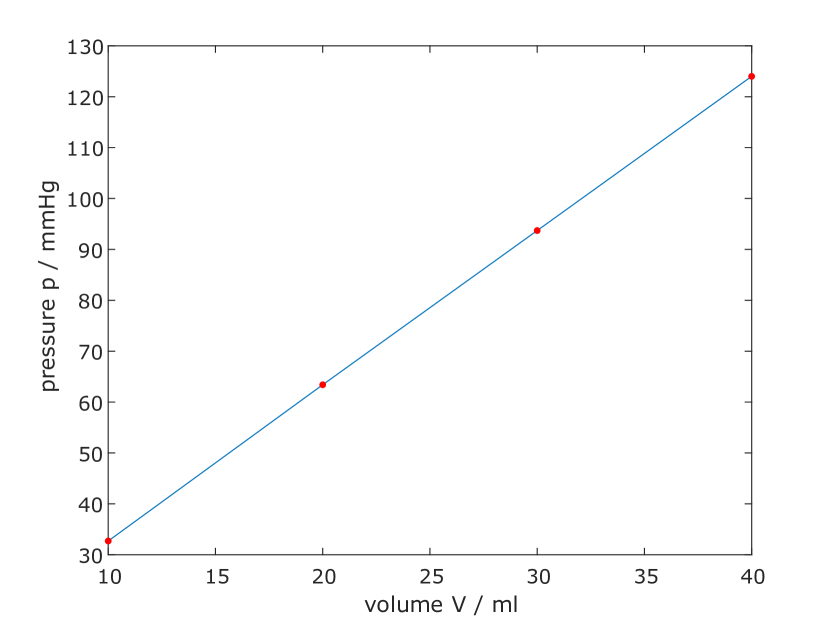
The system compliance was evaluated by measurement of the pressure changes resulting from consecutive fluid injections of into the closed arterial system (see table LABEL:tab:compliance).
| No. | (mmHg) | (ml) | C (ml/mmHg) |
|---|---|---|---|
| 1 | 32,7 | 10 | 0,3058 |
| 2 | 30,7 | 10 | 0,3257 |
| 3 | 30,3 | 10 | 0,3300 |
| 4 | 30,3 | 10 | 0,3300 |
The resulting pressure-volume relation is plotted figure 13, the linear slope implies proportional relationship in the measurement region as expected. Consequently the total arterial compliance can be calculated by equation 5 using the mean pressure difference .
| (5) |
SISCA Model
The node structure of the hardware simulator refers to a computational simulation model realised in the SISCA modelling environment [4]. The node numbering of the arterial tree in SISCA is realised by a depth first search. tree The SISCA software and the simulation model (shown in figure 14) are available at [25].
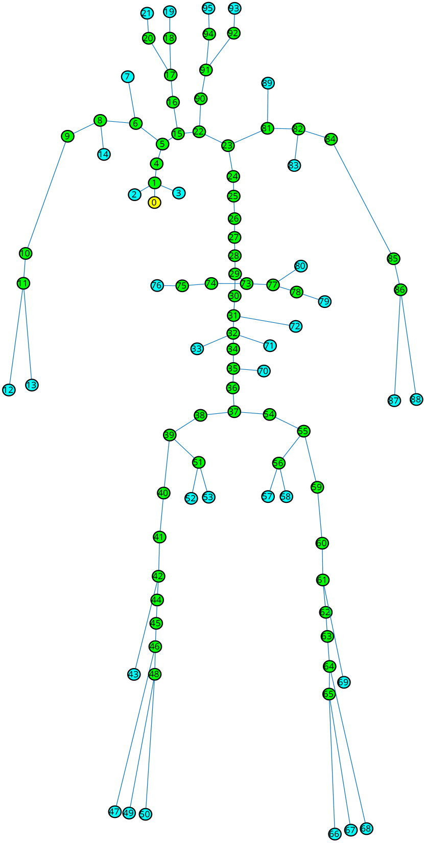
Overview structural properties of the MACSim
Table 5 shows an overview of the properties length l, diameter d, wall thickness h and elasticity E of the corresponding SISCA node ID.
| Node ID | l (m) | h (m) | d (m) | E (Pa) |
|---|---|---|---|---|
| 1 | 0.02 | 0.0015 | 0.025 | 6700000 |
| 2 | 0.067 | 0.0005 | 0.004 | 1650000 |
| 3 | 0.08 | 0.0005 | 0.004 | 1650000 |
| 4 | 0.01 | 0.0015 | 0.025 | 6700000 |
| 5 | 0.052 | 0.0015 | 0.025 | 6700000 |
| 6 | 0.049 | 0.001 | 0.01 | 6700000 |
| 7 | 0.14 | 0.0005 | 0.0015 | 1650000 |
| 8 | 0.016 | 0.001 | 0.01 | 6700000 |
| 9 | 0.053 | 0.001 | 0.01 | 6700000 |
| 10 | 0.35 | 0.001 | 0.006 | 1650000 |
| 11 | 0.021 | 0.001 | 0.004 | 1650000 |
| 12 | 0.325 | 0.001 | 0.004 | 1650000 |
| 13 | 0.345 | 0.0005 | 0.003 | 1650000 |
| 14 | 0.095 | 0.0004 | 0.0015 | 1650000 |
| 15 | 0.013 | 0.0015 | 0.025 | 6700000 |
| 16 | 0.11 | 0.0005 | 0.0065 | 6700000 |
| 17 | 0.045 | 0.0005 | 0.0065 | 6700000 |
| 18 | 0.054 | 0.0005 | 0.004 | 6700000 |
| 19 | 0.036 | 0.0005 | 0.004 | 6700000 |
| 20 | 0.06 | 0.0005 | 0.006 | 6700000 |
| 21 | 0.029 | 0.0005 | 0.006 | 6700000 |
| 22 | 0.012 | 0.0015 | 0.028 | 6700000 |
| 23 | 0.01 | 0.0015 | 0.028 | 6700000 |
| 24 | 0.002 | 0.0015 | 0.028 | 6700000 |
| 25 | 0.05 | 0.0015 | 0.025 | 6700000 |
| 26 | 0.05 | 0.0015 | 0.021 | 6700000 |
| 27 | 0.05 | 0.0015 | 0.02 | 6700000 |
| 28 | 0.049 | 0.0015 | 0.019 | 6700000 |
| 29 | 0.027 | 0.0015 | 0.019 | 6700000 |
| 30 | 0.02 | 0.0015 | 0.018 | 6700000 |
| 31 | 0.006 | 0.0015 | 0.017 | 6700000 |
| 32 | 0.028 | 0.0015 | 0.016 | 6700000 |
| 33 | 0.08 | 0.0005 | 0.004 | 1650000 |
| 34 | 0.021 | 0.0015 | 0.016 | 6700000 |
| 35 | 0.031 | 0.0015 | 0.015 | 6700000 |
| 36 | 0.018 | 0.0015 | 0.015 | 6700000 |
| 37 | 0.015 | 0.0015 | 0.014 | 6700000 |
| 38 | 0.041 | 0.0001 | 0.01 | 6700000 |
| 39 | 0.02 | 0.0001 | 0.01 | 6700000 |
| 40 | 0.094 | 0.0001 | 0.01 | 6700000 |
| 41 | 0.015 | 0.0001 | 0.01 | 6700000 |
| 42 | 0.039 | 0.0001 | 0.008 | 1650000 |
| Node ID | l (m) | h (m) | d (m) | E (Pa) |
|---|---|---|---|---|
| 43 | 0.28 | 0.0005 | 0.003 | 1650000 |
| 44 | 0.13 | 0.0005 | 0.008 | 1650000 |
| 45 | 0.34 | 0.0005 | 0.006 | 1650000 |
| 46 | 0.035 | 0.001 | 0.004 | 1650000 |
| 47 | 0.425 | 0.0005 | 0.002 | 1650000 |
| 48 | 0.049 | 0.001 | 0.004 | 1650000 |
| 49 | 0.375 | 0.0005 | 0.002 | 1650000 |
| 50 | 0.36 | 0.001 | 0.004 | 1650000 |
| 51 | 0.073 | 0.0005 | 0.006 | 6700000 |
| 52 | 0.055 | 0.0005 | 0.006 | 6700000 |
| 53 | 0.063 | 0.0005 | 0.006 | 6700000 |
| 54 | 0.041 | 0.0001 | 0.01 | 6700000 |
| 55 | 0.02 | 0.0001 | 0.01 | 6700000 |
| 56 | 0.073 | 0.0005 | 0.006 | 6700000 |
| 57 | 0.063 | 0.0005 | 0.006 | 6700000 |
| 58 | 0.055 | 0.0005 | 0.006 | 6700000 |
| 59 | 0.094 | 0.0001 | 0.01 | 6700000 |
| 60 | 0.015 | 0.0001 | 0.01 | 6700000 |
| 61 | 0.039 | 0.0001 | 0.008 | 1650000 |
| 62 | 0.13 | 0.0005 | 0.008 | 1650000 |
| 63 | 0.34 | 0.0005 | 0.006 | 4000000 |
| 64 | 0.035 | 0.001 | 0.004 | 1650000 |
| 65 | 0.049 | 0.001 | 0.004 | 1650000 |
| 66 | 0.36 | 0.001 | 0.004 | 1650000 |
| 67 | 0.375 | 0.0005 | 0.002 | 1650000 |
| 68 | 0.425 | 0.0005 | 0.002 | 1650000 |
| 69 | 0.28 | 0.0005 | 0.003 | 1650000 |
| 70 | 0.0167 | 0.0005 | 0.005 | 1650000 |
| 71 | 0.008 | 0.0005 | 0.004 | 1650000 |
| 72 | 0.0175 | 0.0005 | 0.005 | 1650000 |
| 73 | 0.025 | 0.001 | 0.005 | 6700000 |
| 74 | 0.027 | 0.001 | 0.005 | 6700000 |
| 75 | 0.025 | 0.001 | 0.005 | 6700000 |
| 76 | 0.047 | 0.001 | 0.005 | 6700000 |
| 77 | 0.054 | 0.001 | 0.005 | 6700000 |
| 78 | 0.01 | 0.001 | 0.005 | 6700000 |
| 79 | 0.034 | 0.001 | 0.005 | 6700000 |
| 80 | 0.038 | 0.001 | 0.005 | 6700000 |
| 81 | 0.049 | 0.001 | 0.01 | 6700000 |
| 82 | 0.016 | 0.001 | 0.01 | 6700000 |
| 83 | 0.095 | 0.0004 | 0.0015 | 1650000 |
| 84 | 0.053 | 0.001 | 0.01 | 6700000 |
| 85 | 0.35 | 0.001 | 0.006 | 1650000 |
| 86 | 0.021 | 0.001 | 0.004 | 1650000 |
| 87 | 0.345 | 0.0005 | 0.003 | 1650000 |
| 88 | 0.325 | 0.001 | 0.004 | 1650000 |
| 89 | 0.14 | 0.0005 | 0.0015 | 1650000 |
| 90 | 0.11 | 0.0005 | 0.0065 | 6700000 |
| 91 | 0.045 | 0.0005 | 0.0065 | 6700000 |
| 92 | 0.06 | 0.0005 | 0.006 | 6700000 |
| 93 | 0.029 | 0.0005 | 0.006 | 6700000 |
| 94 | 0.054 | 0.0005 | 0.004 | 6700000 |
| 95 | 0.036 | 0.0005 | 0.004 | 6700000 |
Peripheral Resistance Measurement
The peripheral resistances were measured by the definition of different regional groups (see table 1). The peripheral resistance, , of each group was determined by the volume difference between the steady state and running system. Volume integration was done by disconnection of the reservoirs and determination of the fluid amount per time. Only the corresponding arteries in the defined group were connected to the arterial network of the simulator by closing all 3-way valves to other arteries. Given the volume and pressure difference, the peripheral resistance for each group was calculated by using equation 1.
The peripheral resistance is build by different elements (see figure 4), which all possess static values, except the resistance of the small inner tubes is varying according to their length. In table 6 the length of the small inner tubes to the corresponding boundary node ID is shown.
| Node ID | (mm) |
|---|---|
| 2 | 19.8 |
| 3 | 19.4 |
| 12 | 7 |
| 13 | 8.3 |
| 19 | 2.4 |
| 21 | 2.7 |
| 33 | 19.5 |
| 43 | 13 |
| 47 | 8.3 |
| 49 | 17.6 |
| 50 | 17.2 |
| 52 | 19.4 |
| 53 | 19.4 |
| 57 | 19.4 |
| 58 | 19.5 |
| 66 | 17.6 |
| 67 | 17.2 |
| 68 | 4.7 |
| 69 | 13.3 |
| 70 | 8.3 |
| 71 | 19.4 |
| 72 | 8.2 |
| 76 | 8.4 |
| 79 | 5.4 |
| 80 | 8.4 |
| 87 | 8.9 |
| 88 | 7 |
| 93 | 2.3 |
| 95 | 2.1 |
| 7 | / |
| 89 | / |
| 14 | / |
| 83 | / |