General Time-Dependent Configuration-Interaction Singles
I: The Molecular Case

Abstract

We present a grid-based implementation of the time-dependent configuration-interaction singles method suitable for computing the strong-field ionization of small gas-phase molecules. After outlining the general equations of motion used in our treatment of this method, we present example calculations of strong-field ionization of He, LiH, H2O, and C2H4 that demonstrate the utility of our implementation. The following companion paper [1] specializes to the case of spherical symmetry, which is applied to various atoms.

I.1 Introduction

Strong-field physics and attosecond science offer a rich experimental platform to study ultrafast phenomena on electronic time and length scales [2, 3]. Applied to gas phase molecules, techniques such as high-harmonic spectroscopy [4, 5, 6, 7, 8], orbital tomography [9], laser-induced electron diffraction [10, 11, 12] and holography [13], attempt to use the technologies of attosecond physics to probe electronic structures and dynamics that occur within molecular systems. Although promising, fine-tuning these techniques to extract accurate and complete information is not straight-forward due to the highly non-linear and non-perturbative nature of the strong-field interactions driving these experimental efforts. Often the only path to disentangling and interpreting the measurable experimental observables is through detailed modeling of not only the underlying molecular and electronic structures but also the complete probing process itself. In this regard, the novel spectroscopic methods brought forth by strong-field and attosecond physics will only be as accurate as the underlying modeling used to interpreting the complex observables involved.

The first step in all of these strong-field driven processes is the removal of an electron with a strong low-frequency laser field. Following ionization, the liberated electron is then accelerated in the laser field and driven back to recollide with the parent ion, a process called laser-induced electron recollision. In order to accurately describe this time-dependent non-perturbative process at an ab initio level, it is necessary to develop time-domain methods that can interface with standard methods in time-independent electronic structure theory. In addition, a proper description of the recollision motion of the continuum electron will likely require going beyond the localized Gaussian-like basis sets upon which most of standard electronic structure codes are based. In this article, we develop and explore a grid-based implementation of Time-Dependent Configuration-Interaction Singles (TD-CIS) as applied to small gas-phase molecules, where Cartesian grids are used to represent the continuum electron, while still using Gaussians for the occupied orbitals.

The problems we are interested in studying are not new, and many different approaches have been fruitfully pursued before. A listing, that is by no means exhaustive, would include TD-CIS for molecules [14, 15, 16, 17, 18, 19, 20], TD-CIS for atoms [21, 22], a newly developed relativistic TD-CIS, RTDCIS that takes the Dirac equation as its starting point [23]; Time-Dependent Density-Functional Theory [24, 25, 26, 27]; methods that go beyond the single Slater determinant Ansatz, such as Multiconfigurational Time-Dependent Hartree [28, 29, 30], Multiconfigurational Time-Dependent Hartree–Fock [31, 32, 33, 34, 35], Time-Dependent Multiconfigurational Self-Consistent-Field [36]; Time-Dependent Complete-Active-Space Self-Consistent-Field [37]; Time-Dependent Resolution in Ionic States [38]; the various restricted active space methods, e.g. Time-Dependent Restricted-Active-Space Configuration-Interaction [39] and Time-Dependent Occupation-Restriction Multiple-Active-Space [40]; the excitation-class based methods Time-Dependent Coupled-Cluster [41, 42, 43] and Algebraic Diagrammatic Construction [44, 45, 46]; and finally we mention the recent extension of the R-matrix method to molecules, UKRmol+ [47] and RMT [48]. For reviews of the various ab initio approaches to multielectron dynamics, see Ishikawa and Sato [49], Armstrong et al. [50].

This article is arranged as follows: in section I.2, the general equations of motion for the TD-CIS Ansatz are derived in detail, as well as the generalization of surface-flux techniques to compute photoelectron spectra to multiple ionization channels. The time propagator is briefly surveyed in section I.3, and some illustrative calculations are presented in section I.4. Finally, section I.5 concludes the paper.

I.1.1 Conventions

Hartree atomic units where $\hbar=e=a_{0}=m_{\mathrm{e}}=1$ are used throughout.

We employ a modified version of Einstein’s summation convention, where indices appearing on one side of an equality sign only are automatically contracted over, e.g.

$$\Psi=c_{0}\Phi_{0}+\tilde{\Phi}_{k}\equiv c_{0}\Phi_{0}+\sum_{k}\tilde{\Phi}_{k}.$$

For the canonical orbitals, we use the following letters:

• $\ket{i}$, $\ket{j}$, $\ket{k}$, $\ket{l}$ denote occupied orbitals,

• $\ket{a}$, $\ket{b}$ denote virtual orbitals,

• $\ket{c}$, $\ket{d}$, $\ket{e}$, $\ket{f}$ denote any orbitals.

Matrix elements between orbitals are written using Mulliken-like notation:

$$(c|d) \overset{\textrm{\tiny def}}{=}\matrixelement{c}{\hat{h}_{0}+\hat{V}_{L}(t)}{d},$$ (I–1)

$$[cd||ef] \overset{\textrm{\tiny def}}{=}[cd|ef]-[cd|fe];$$

$$[cd|ef] \overset{\textrm{\tiny def}}{=}\int\frac{\mathrm{d}\varsigma_{1}\;\mathrm{d}\varsigma_{2}\;}{\absolutevalue{\mathbf{r}_{1}-\mathbf{r}_{2}}}\chi_{c}^{*}(\varsigma_{1})\chi_{d}^{*}(\varsigma_{2})\chi_{e}(\varsigma_{1})\chi_{f}(\varsigma_{2}),$$

where $\hat{h}_{0}\overset{\textrm{\tiny def}}{=}\hat{T}+\hat{V}$ is the molecular one-body Hamiltonian, and $\hat{V}_{L}(t)$ is the time-dependent potential due to the external laser field. $\varsigma_{1,2}$ refer to both spatial and spin coordinates of the orbitals.

I.2 General TD-CIS, equations and surface flux

Our Ansatz is

$$\Psi(t)=c_{0}(t)\Phi_{0}+\tilde{\Phi}_{k}(t),$$ (I–2)

where $\Phi_{0}$ is the Slater determinant of the reference state (typically the Hartree–Fock ground state), $c_{0}(t)$ is time-dependent complex amplitude, and $\tilde{\Phi}_{k}(t)$ an excited Slater determinant obtained by substituting the occupied orbital $\ket{k}$ of the reference by a time-dependent particle orbital $\ket*{\tilde{k}}$ formed as a linear combination of the virtual canonical orbitals:

$$\tilde{\Phi}_{k}(t)\overset{\textrm{\tiny def}}{=}c_{ka}(t)\hat{a}^{\dagger}_{a}\hat{a}_{k}\Phi_{0}\implies\ket*{\tilde{k}}=c_{ka}(t)\ket{a}.$$

No distinction is made between excitation and ionization channels, since $\ket*{\tilde{k}}$ is associated with a particular hole configuration of the remaining ion, the particle–hole density of which is given by $\outerproduct*{\tilde{k}}{k}$. We also note that this implies that particle orbitals corresponding to different occupied orbitals are non-orthogonal, $\innerproduct*{\tilde{k}}{\tilde{l}}\neq 0$, which must be taken into account when forming the energy expression [51].

To derive the equations of motion (EOMs), we start from the Dirac–Frenkel variational principle:

$$\delta_{\bra{\Psi}}\hat{L}=0,$$ (I–3)

where the Lagrangian is given by

$$\hat{L}=\matrixelement{\Psi}{\hat{H}-\mathrm{i}\partial_{t}}{\Psi}-\lambda_{i\tilde{j}}\innerproduct*{i}{\tilde{j}}-\lambda_{\tilde{j}i}\innerproduct*{\tilde{j}}{i}.$$ (I–4)

The Lagrange multipliers $\lambda_{i\tilde{j}},\lambda_{\tilde{j}i}$ ensure that the particle orbitals $\ket*{\tilde{j}}$ remain orthogonal to the occupied orbitals $\ket{i}$ at all times; this is necessary since otherwise the basis would be overcomplete. In the time propagation, they are implemented as projectors, without explicitly evaluating the multipliers. A possible alternative approach would have been to treat the Lagrange multipliers as dynamical variables [52]. Such a formulation avoids an explicit orthogonalization step, quadratic in the number of orbitals, leading to substantial efficiency improvements in effective one-electron theories such as TD-DFT. The potential savings are however likely to remain minor in wavefunction-based methods such as TD-CIS.

Inserting the Ansatz (I–2) into the expression (I–4) for the Lagrangian, we find

$$\hat{L}=E-c_{0}^{*}\mathrm{i}\partial_{t}c_{0}-\matrixelement*{\tilde{k}}{\mathrm{i}\partial_{t}}{\tilde{k}}-\lambda_{i\tilde{j}}\innerproduct*{i}{\tilde{j}}-\lambda_{\tilde{j}i}\innerproduct*{\tilde{j}}{i},$$ (I–5)

where the total energy is given by

$$E =\absolutevalue{c_{0}}^{2}E_{0}+\innerproduct*{\tilde{k}}{\tilde{k}}E_{k}+{\color[rgb]{0,0,1}(c_{0}^{*}E_{k\tilde{k}}+\textrm{c.c.})}$$

$$\hphantom{=}+{\color[rgb]{0,0.5,0.5}E_{\tilde{k}\tilde{k}}}-\innerproduct*{\tilde{k}}{\tilde{l}}{\color[rgb]{1,0,0}E_{lk}}-{\color[rgb]{1,0.5,0}[l\tilde{k}||k\tilde{l}]}.$$

We have here introduced the following notation for the partial contributions to the overall energy:

$$E_{0}\overset{\textrm{\tiny def}}{=}(i|i)+\frac{1}{2}[ij||ij]$$

is the (time-dependent) energy of the reference determinant $\Phi_{0}$,

$$E_{k}\overset{\textrm{\tiny def}}{=}E_{0}-\epsilon_{k}$$

the channel energy associated with excitation/ionization from the occupied orbital $k$, and the orbital energy

$$\epsilon_{k}\overset{\textrm{\tiny def}}{=}\epsilon_{kk},\quad\epsilon_{kl}\overset{\textrm{\tiny def}}{=}(k|l)+\frac{1}{2}[kj||lj].$$

The occupied–virtual orbital energy (and its complex conjugate)

$${\color[rgb]{0,0,1}E_{k\tilde{k}}\overset{\textrm{\tiny def}}{=}(k|\tilde{k})+[ki||\tilde{k}i]}$$

contain the terms that lead to excitation/ionization from the reference, whereas the virtual–virtual energy

$${\color[rgb]{0,0.5,0.5}E_{\tilde{k}\tilde{k}}\overset{\textrm{\tiny def}}{=}(\tilde{k}|\tilde{k})+[\tilde{k}i||\tilde{k}i]}$$

describe the interaction of the excited/ionized electron with its parent ion state (intrachannel) as well as with the external field. Finally, the interchannel energies

$${\color[rgb]{1,0,0}E_{lk}\overset{\textrm{\tiny def}}{=}(l|k)+[li||ki]};\quad{\color[rgb]{1,0.5,0}[l\tilde{k}||k\tilde{l}]}$$

describe coupling between the various ionization channels through the external field and Coulomb interaction, respectively. We note that due to the linearity of the Ansatz (I–2), we are free to choose the energy origin; by setting $E_{0}=0$, we avoid having to converge the quick phase evolution due to the HF reference. Simultaneously, the channel energy becomes simply $E_{k}=-\epsilon_{k}$.

By varying (I–5) with respect to $c_{0}^{*}$ and $\bra*{\tilde{k}}$, we get the EOMs:

$$\mathrm{i}\partial_{t}c_{0} =c_{0}E_{0}+{\color[rgb]{0,0,1}\matrixelement*{k}{\hat{f}missing}{\tilde{k}}},$$ (I–6)

$$\mathrm{i}\partial_{t}\ket*{\tilde{k}} =(E_{k}+{\color[rgb]{0,0.5,0.5}\hat{f}})\ket*{\tilde{k}}+{\color[rgb]{0,0,1}c_{0}\hat{f}\ket{k}}$$

$$\hphantom{=}-{\color[rgb]{1,0,0}\matrixelement{l}{\hat{f}missing}{k}}\ket*{\tilde{l}}-{\color[rgb]{1,0.5,0}(\hat{J}_{lk}-\hat{K}_{lk})\ket*{\tilde{l}}}-\lambda_{\tilde{k}i}\ket{i},$$

where the Fock operator is defined as

$$\hat{f}\overset{\textrm{\tiny def}}{=}\hat{h}_{0}+\hat{V}_{L}(t)+\hat{J}_{ii}-\hat{K}_{ii},\implies\matrixelement{l}{\hat{f}missing}{k}\equiv\epsilon_{lk},$$

and the direct and exchange potentials by their action on an orbital:

$$\hat{J}_{cd}\ket{e} \overset{\textrm{\tiny def}}{=}\chi_{e}(\varsigma_{1})\int\frac{\mathrm{d}\varsigma_{2}\;}{\absolutevalue{\mathbf{r}_{1}-\mathbf{r}_{2}}}\chi_{c}^{*}(\varsigma_{2})\chi_{d}(\varsigma_{2}),$$

$$\hat{K}_{cd}\ket{e} \overset{\textrm{\tiny def}}{=}\chi_{d}(\varsigma_{1})\int\frac{\mathrm{d}\varsigma_{2}\;}{\absolutevalue{\mathbf{r}_{1}-\mathbf{r}_{2}}}\chi_{c}^{*}(\varsigma_{2})\chi_{e}(\varsigma_{2})\equiv\hat{J}_{ce}\ket{d}.$$

We now use our gauge freedom to choose $E_{0}=0$, and we get the modified EOMs

$$\mathrm{i}\partial_{t}c_{0} ={\color[rgb]{0,0,1}\matrixelement*{k}{\hat{f}missing}{\tilde{k}}},$$ (I–7)

$$\mathrm{i}\partial_{t}\ket*{\tilde{k}} =(-\matrixelement{k}{\hat{f}missing}{k}+{\color[rgb]{0,0.5,0.5}\hat{f}})\ket*{\tilde{k}}+{\color[rgb]{0,0,1}c_{0}\hat{f}\ket{k}}$$

$$\hphantom{=}-{\color[rgb]{1,0,0}\matrixelement{l}{\hat{f}missing}{k}}\ket*{\tilde{l}}-{\color[rgb]{1,0.5,0}(\hat{J}_{lk}-\hat{K}_{lk})\ket*{\tilde{l}}}-\lambda_{\tilde{k}i}\ket{i},$$

If $\ket{k}$ and $\ket*{\tilde{k}}$ live in different vector spaces, e.g. if $\ket{k}$ is expanded in a basis set of Gaussians and $\ket*{\tilde{k}}$ is resolved on a grid, their respective matrix representations of the Fock operator $\hat{f}$ will in general not agree, i.e. $\ket{k}$ resolved on the grid of $\ket*{\tilde{k}}$ will not necessarily be an eigenvector of the matrix representation of $\hat{f}$ on the same grid. It is therefore important to compute matrix elements of operators in the correct vector space. The chief reason for representing the occupied orbitals using Gaussians instead of resolving them on the grid and computing the matrix elements of the Fock operator accordingly, is that any grid coarse enough to be reasonable for time propagation would not be able to accurately represent the oscillatory behaviour of the Fock operator close to the nuclei. Specifically, the direct interaction $\hat{J}_{ii}$ needs to partially screen the nuclear potentials $-Z_{B}/\absolutevalue{\mathbf{R}_{B}-\mathbf{r}_{i}}$ such that the long range potential behaves as $-1/r_{i}$. This cancellation is challenging to achieve accurately on a coarse grid, while it is trivial to compute exactly in the Gaussian basis and then instantiate the result on the grid. A similar argument can be made for the short-range, non-local potential $\hat{J}_{ii}-\hat{K}_{ii}$.

If instead $\ket{k}$ and $\ket*{\tilde{k}}$ do live in the same vector space, we may choose $\ket{k},\ket{l}...$ to be the canonical orbitals which diagonalize the field-free Fock operator. This choice (which we make in the special case of atomic symmetry; see the following article) is a restriction compared to the more general case considered in this article. Furthermore, in case of an atom placed at the origin of our coordinate system, there are no permanent dipole moments. These two restrictions considerably simplify the EOMs:

$$\mathrm{i}\partial_{t}c_{0} ={\color[rgb]{0,0,1}\matrixelement*{k}{\hat{V}_{L}missing}{\tilde{k}}},$$ (I–8)

$$\mathrm{i}\partial_{t}\ket*{\tilde{k}} =(-\epsilon_{k}+{\color[rgb]{0,0.5,0.5}\hat{f}})\ket*{\tilde{k}}+{\color[rgb]{0,0,1}c_{0}\hat{V}_{L}\ket{k}}$$

$$\hphantom{=}-{\color[rgb]{1,0,0}\matrixelement{l}{\hat{V}_{L}missing}{k}}\ket*{\tilde{l}}-{\color[rgb]{1,0.5,0}(\hat{J}_{lk}-\hat{K}_{lk})\ket*{\tilde{l}}}-\lambda_{\tilde{k}i}\ket{i},$$

where we have dropped the term ${\color[rgb]{0,0,1}c_{0}(\hat{h}_{0}+\hat{J}_{ii}-\hat{K}_{ii})\ket{k}}$ since we require $\innerproduct*{k}{\tilde{k}}=0$. Our molecular implementation below uses (I–7), while our atomic implementation [1] relies on (I–8).

I.2.1 t+iSURF{C,V}

The following derivation in similar in spirit to Scrinzi [53], Orimo et al. [54], but differs in the details.

We begin by defining the $N$-electron Heaviside function acting on one electron:

$$\Theta\overset{\textrm{\tiny def}}{=}\hat{\Pi}_{jN}[1-\theta(r_{1}-R_{\textrm{s}})]...[1-\theta(r_{N-1}-R_{\textrm{s}})]\theta(r_{N}-R_{\textrm{s}}),$$ (I–9)

where $\hat{\Pi}_{jN}$ permutes coordinates $j$ and $N$. With this, we construct our Ansatz for the asymptotic region ($r_{j}>R_{\textrm{s}}$):

$$\Theta\ket{\Psi(t)} =a_{n}(\mathbf{p}_{\sigma_{z}},t)\mathcal{A}\ket{\xi_{n}(t)}\ket{\mathbf{p}_{\sigma_{z}}(t)}$$

$$\overset{\textrm{\tiny def}}{=}a_{n}(\mathbf{p}_{\sigma_{z}},t)\ket{\xi_{n}(t)\mathbf{p}_{\sigma_{z}}(t)},$$

where $\{\ket{\xi_{n}(t)}\}$ is a “time-dependent, complete but otherwise arbitrary set of functions” [53] that spans the ion degrees of freedom, and $\ket{\mathbf{p}_{\sigma_{z}}(t)}$ is an electron with final momentum $\mathbf{p}$ and spin projection ${\sigma_{z}}$.

The antisymmetrization operator used above to couple an already antisymmetrized ($N-1$)-body wavefunction $\ket{\xi_{n}(t)}$ with one electron $\ket{\mathbf{p}_{\sigma_{z}}(t)}$ to form an antisymmetrized $N$-body wavefunction is defined as

$$\mathcal{A}\overset{\textrm{\tiny def}}{=}\frac{1}{\sqrt{N}}(-)^{N-j}\hat{\Pi}_{jN},$$ (I–10)

where $(-)^{N-j}$ is the signature of the permutation. This form is valid, provided that the strong orthogonality assumption applies, i.e. that the scattering state $\ket{\mathbf{p}_{\sigma_{z}}(t)}$ is orthogonal to all the bound orbitals of the initial state [55, 56, 57, 58]. This condition is trivially fulfilled due to the presence of the Heaviside function (I–9).

The overlap with such an asymptotic state is given by

$$a_{n}(\mathbf{p}_{\sigma_{z}},t) =\matrixelement{\xi_{n}(t)\mathbf{p}_{\sigma_{z}}(t)}{\Theta}{\Psi(t)}$$ (I–11)

$$=\bra{\xi_{n}(t)}\!\!\matrixelement{\mathbf{p}_{\sigma_{z}}(t)}{\mathcal{A}\Theta}{\Psi(t)}$$

$$={\color[rgb]{0,0,1}\bra{\mathbf{p}_{\sigma_{z}}(t)}}\theta\sqrt{N}\left\langle{\color[rgb]{1,0,0}\xi_{n}(t)}\middle|{\color[rgb]{0,0.5,0.5}\Psi(t)}\right\rAngle$$

$$\overset{\textrm{\tiny def}}{=}\matrixelement{{\color[rgb]{0,0,1}{\mathbf{p}_{\sigma_{z}}(t)}}}{\theta}{n(t)},$$

where we have used the fact that $\mathcal{A}$ is self-adjoint to act with it on $\Theta\ket{\Psi(t)}$ to the right, and that only $N$ terms are non-zero for which the coordinate of $\ket{\mathbf{p}_{\sigma_{z}}(t)}$ coincides with the photoelectron orbital in $\ket{\Psi(t)}$ (a single orbital in TD-CIS). The sign of each such term will precisely compensate the corresponding sign of the antisymmetrizer (I–10). The normalization leaves a factor of $\sqrt{N}$, which is absorbed into the definition of the Dyson orbital $\ket{n(t)}$. Finally, $\rAngle$ denotes integration over both the photoelectron and ion coordinates. The benefit of formulating the photoelectron amplitudes in terms of Dyson orbitals is that the various surface terms then attain the familiar expressions from the single-electron case, with the Dyson orbital replacing the single-electron wavefunction. The only remaining difference is in the channel coupling through the ion Hamiltonian.

It is convenient to choose $\ket{\xi_{n}(t)}$ as the time-dependent eigenstates of the ion:

$$\ket{\xi_{n}(t)} \overset{\textrm{\tiny def}}{=}\mathrm{e}^{-\mathrm{i}E_{n}(t-t_{i})}\ket{\xi_{n}}$$

$$\implies\bra{\xi_{n}(t)}[\mathrm{i}\partial_{t}^{\dagger}+E_{n}] \equiv\bra{\xi_{n}(t)}[\mathrm{i}\partial_{t}^{\dagger}+\hat{H}_{\textrm{ion}}]=0,$$

where $t_{i}$ is some reference time, usually taken as the beginning of the laser interaction.

Similarly, the scattering states obey the one-electron TDSE

$$\bra{\mathbf{p}_{\sigma_{z}}(t)}[\mathrm{i}\partial_{t}^{\dagger}+\hat{h}_{S}]=0$$

and the wavefunction in the asymptotic region

$$[\mathrm{i}\partial_{t}-(\hat{H}_{\textrm{ion}}+\hat{h}_{S})]\ket{\Psi(t)}=0.$$

The EOMs for the overlaps (I–11) are then

$$-\mathrm{i}\partial_{t}a_{n}(\mathbf{p}_{\sigma_{z}},t) ={\color[rgb]{0,0,1}\bra{\mathbf{p}_{\sigma_{z}}(t)}\!\hat{h}_{S}\theta\sqrt{N}\!\left\langle\xi_{n}(t)\middle|\Psi(t)\right\rAngle}+{\color[rgb]{1,0,0}E_{n}\bra{\mathbf{p}_{\sigma_{z}}(t)}\!\theta\sqrt{N}\!\left\langle\xi_{n}(t)\middle|\Psi(t)\right\rAngle}-{\color[rgb]{0,0.5,0.5}\bra{\mathbf{p}_{\sigma_{z}}(t)}\!\theta\sqrt{N}\langle\xi_{n}(t)|\hat{H}_{\textrm{ion}}(t)+\hat{h}_{S}|\Psi(t)\rAngle}$$

$$={\color[rgb]{1,0,0}E_{n}a_{n}(\mathbf{p}_{\sigma_{z}},t)}-{\color[rgb]{0,0.5,0.5}\bra{\mathbf{p}_{\sigma_{z}}(t)}\theta\sqrt{N}\!\langle\xi_{n}(t)|\hat{H}_{\textrm{ion}}(t)\hat{\mathbf{1}}|\Psi(t)\rAngle}+\matrixelement*{\mathbf{p}_{\sigma_{z}}(t)}{{\color[rgb]{0,0,1}\hat{h}_{S}\theta}-{\color[rgb]{0,0.5,0.5}\theta\hat{h}_{S}}}{n(t)}$$

$$={\color[rgb]{1,0,0}E_{n}a_{n}(\mathbf{p}_{\sigma_{z}},t)}-{\color[rgb]{0,0.5,0.5}\underbrace{\matrixelement{\xi_{n}(t)}{\hat{H}_{\textrm{ion}}(t)}{\xi_{m}(t)}}_{\overset{\textrm{\tiny def}}{=}\mathsf{H}_{nm}(t)}\underbrace{\matrixelement{\mathbf{p}_{\sigma_{z}}(t)}{\theta}{\mathbf{q}_{{\sigma_{z}}^{\prime}}(t)}}_{\delta(\mathbf{p}-\mathbf{q})\delta_{{\sigma_{z}}{\sigma_{z}}^{\prime}}}a_{m}(\mathbf{q}_{{\sigma_{z}}^{\prime}},t)}+\underbrace{\matrixelement*{\mathbf{p}_{\sigma_{z}}(t)}{\commutator*{\hat{h}_{S}}{\theta}}{n(t)}}_{S_{n}(\mathbf{p}_{\sigma_{z}},t)}$$

$$=-\tilde{\mathsf{H}}_{nm}(t)a_{m}(\mathbf{p}_{\sigma_{z}},t)+S_{n}(\mathbf{p}_{\sigma_{z}},t),$$

where the ionic Hamiltonian in the interaction picture is given by

$$\tilde{\mathsf{H}}_{nm}(t) \overset{\textrm{\tiny def}}{=}\mathsf{H}_{nm}(t)-\delta_{nm}E_{n},$$

$$\mathsf{H}_{nm}(t) =\matrixelement{\xi_{n}(t)}{\hat{H}_{\textrm{ion}}(t)}{\xi_{m}(t)}$$

$$=\mathrm{e}^{\mathrm{i}E_{nm}t}[\delta_{nm}E_{n}+\matrixelement{\xi_{n}}{\hat{V}_{L}(t)}{\xi_{m}}],$$

$$E_{nm} =E_{n}-E_{m},$$

and the asymptotic resolution of identity by

$$\hat{\mathbf{1}}=\ket{\xi_{m}(t)}\outerproduct{\mathbf{q}_{{\sigma_{z}}^{\prime}}(t)}{\mathbf{q}_{{\sigma_{z}}^{\prime}}(t)}\bra{\xi_{m}(t)}.$$

The EOMs can be written on matrix form

$$-\mathrm{i}\partial_{t}\mathbf{a}(\mathbf{p}_{\sigma_{z}},t)=-\tilde{\mathsf{H}}(t)\mathbf{a}(\mathbf{p}_{\sigma_{z}},t)+\mathbf{S}(\mathbf{p}_{\sigma_{z}},t).$$ (I–12)

$S_{n}(\mathbf{p}_{\sigma_{z}},t)$ is the surface term contributing to ionization channel $n$ and final photoelectron momentum $\mathbf{p}$ and spin projection ${\sigma_{z}}$. The precise form of the surface terms depends on the asymptotic wavefunction chosen (e.g. Coulomb or Volkov scattering wavefunctions), as well as the gauge [59, 60].

Rearranging, we get

$$\partial_{t}\mathbf{a}(\mathbf{p}_{\sigma_{z}},t)+\mathrm{i}\tilde{\mathsf{H}}(t)\mathbf{a}(\mathbf{p}_{\sigma_{z}},t)=\mathrm{i}\mathbf{S}(\mathbf{p}_{\sigma_{z}},t),$$ (I–13)

which is an inhomogeneous differential equation for the photoionization amplitude $\mathbf{a}(\mathbf{p}_{\sigma_{z}},t)$. If we discretize (I–13) in time and apply the trapezoidal rule, evaluating the ionic Hamiltonian at half the time step, we find (suppressing the dependence on $\mathbf{p}_{\sigma_{z}}$)

$$\frac{\mathbf{a}_{i+1}-\mathbf{a}_{i}}{\tau}+\frac{\mathrm{i}}{2}(\tilde{\mathsf{H}}_{i+1/2}\mathbf{a}_{i+1}+\tilde{\mathsf{H}}_{i+1/2}\mathbf{a}_{i})=\frac{\mathrm{i}}{2}(\mathbf{S}_{i+1}+\mathbf{S}_{i})$$ (I–14)

$$\iff\left(\hat{\mathbf{1}}+\frac{\mathrm{i}\tau}{2}\tilde{\mathsf{H}}_{i+1/2}\right)\mathbf{a}_{i+1}=$$

$$\qquad\qquad\left(\hat{\mathbf{1}}-\frac{\mathrm{i}\tau}{2}\tilde{\mathsf{H}}_{i+1/2}\right)\mathbf{a}_{i}+\frac{\mathrm{i}\tau}{2}(\mathbf{S}_{i}+\mathbf{S}_{i+1}),$$

which is globally accurate to $\mathcal{O}\{\tau^{2}\}$.

I.2.1.1 Diagonal $\tilde{\mathsf{H}}$

If $\tilde{\mathsf{H}}$ is diagonal (and time-independent), its elements are zero, no channel-coupling occurs, and we can integrate each component of (I–13) separately:

$$a_{n}(\mathbf{p}_{\sigma_{z}},t) =\mathrm{i}\int_{t_{i}}^{t}\mathrm{d}\tau\;S_{n}(\mathbf{p}_{\sigma_{z}},\tau)$$ (I–15)

$$=\mathrm{i}\int_{t_{i}}^{t}\mathrm{d}\tau\;\bra{\mathbf{p}_{\sigma_{z}}(\tau)}\commutator*{\hat{h}_{S}}{\theta}\ket{n(\tau)},$$

and we recover Koopman’s theorem [since $\ket{\xi_{n}(\tau)}\equiv\mathrm{e}^{-\mathrm{i}E_{n}(\tau-t_{i})}\ket{\xi}$], which is an excellent approximation in CIS, if promotions are allowed from the valence shell only.

I.2.1.2 iSURF

In the case of a discretized spectrum [61], the time evolution of the wavefunction after the end of the pulse ($t=t_{f}$) is trivially given by

$$\ket{\Psi(t>t_{f})}=\ket{\gamma}\innerproduct*{\gamma}{\Psi(t_{f})}\mathrm{e}^{-\mathrm{i}E_{\gamma}(t-t_{f})}$$ (I–16)

where $\gamma$ represents all quantum numbers necessary to describe an eigenstate of the field-free Hamiltonian $\hat{H}_{0}$, and $E_{\gamma}$ is its eigenenergy, which will have a negative imaginary part in the presence of absorbing boundary conditions (corresponding to exponential decay of outgoing waves). Furthermore, after the pulse has ended, $\tilde{\mathsf{H}}$ is diagonal, i.e. there is no coupling between the ionization channels anymore, and only the surface term remains, and the amplitude is given by (I–15). Integrating this amplitude from the end of the pulse $t_{f}$ to the detection time (suppressing the $\mathbf{p}_{\sigma_{z}}$ argument), we find

$$a_{n}(\infty)-a_{n}(t_{f})=\mathrm{i}\int_{t_{f}}^{\infty}\mathrm{d}\tau\;\bra{\mathbf{p}_{\sigma_{z}}(\tau)}\commutator*{\hat{h}_{S}}{\theta}\ket{n(\tau)}.$$

The total amplitude for channel $n$ will be given by

$$a_{n}(\infty) =a_{n}(t_{f})+[a_{n}(\infty)-a_{n}(t_{f})]$$

$$=\underbrace{a_{n}(t_{f})}_{\textrm{tSURFF}}+\underbrace{\mathrm{i}\int_{t_{f}}^{\infty}\mathrm{d}\tau\;S_{n}(\tau)}_{\textrm{iSURF}}.$$

Inserting the Ansatz (I–16) into the source term, we find

$$S_{n}(\mathbf{p}_{\sigma_{z}},t>t_{f})=\bra{\mathbf{p}_{\sigma_{z}}(t)}\commutator*{\hat{h}_{S}}{\theta}\ket{n(t)}$$

$$\quad=\bra{\mathbf{p}_{\sigma_{z}}(t)}\commutator*{\hat{h}_{S}}{\theta}\sqrt{N}\innerproduct{\xi_{n}(t)}{\gamma}\left\langle\gamma\middle|\Psi(t_{f})\right\rAngle\mathrm{e}^{\mathrm{i}(\epsilon-E_{\gamma})(t-t_{f})},$$

where the target energy is chosen as $\epsilon\overset{\textrm{\tiny def}}{=}E_{n}+p^{2}/2$. By identical manipulations as in Equations (14–17) of Morales et al. [60], and assuming the existence of the operator inverse, we arrive at

$$a_{n}(\infty)-a_{n}(t_{f})=\matrixelement{\mathbf{p}_{\sigma_{z}}(t_{f})}{\commutator*{\hat{h}_{S}}{\theta}}{n(\epsilon)},$$ (I–17)

where the Dyson orbital is given by

$$\ket{n(\epsilon)}=\sqrt{N}\innerproduct{\xi_{n}(t_{f})}{\Omega(\epsilon)},\quad\ket{\Omega(\epsilon)}\overset{\textrm{\tiny def}}{=}(\hat{H}_{0}-\epsilon)^{-1}\ket{\Psi(t_{f})},$$

and $\ket{\Omega(\epsilon)}$ is found using GMRES [62], with the $\hat{h}-\epsilon$ as the preconditioner. We stress that Equations (I–13), (I–14), and (I–17) are valid for single ionization for any Ansatz, and not just TD-CIS (I–2).

I.2.1.3 Surface terms, gauge dependence

The surface terms require the evaluation of

$$S_{n}(\mathbf{p}_{\sigma_{z}},t)=\matrixelement*{\mathbf{p}_{\sigma_{z}}(t)}{\commutator*{\hat{h}_{S}}{\theta}}{n(t)},$$

which depends on the particular form of scattering wavefunctions chosen, as well as the gauge:

$$\hat{h}_{S}=\hat{T}+\hat{V}_{L}(t)=\hat{T}+\begin{cases}\mathbf{F}(t)\cdot\mathbf{r},&\textrm{(length gauge)},\\ \mathbf{A}(t)\cdot\mathbf{p},&\textrm{(velocity gauge)},\end{cases}$$ (I–18)

$$\implies\commutator*{\hat{h}_{S}}{\theta}=\commutator*{\hat{T}}{\theta}+\begin{cases}0,&\textrm{(length gauge)},\\ \commutator*{\mathbf{A}(t)\cdot\mathbf{p}}{\theta},&\textrm{(velocity gauge)}.\end{cases}$$

tSURFF has customarily been used in the velocity gauge, which is valid since the SAE approximation is gauge invariant (provided only local potentials are used) [59, 60]. In this gauge, the Volkov scattering wavefunctions have the simple expression

$$\chi^{\mathrm{V}}_{\mathbf{p}v}(t,\mathbf{r})=\frac{1}{(2\pi)^{3/2}}\exp\left\{\mathrm{i}\mathbf{p}\cdot\mathbf{r}-\frac{\mathrm{i}}{2}\int_{t_{0}}^{t}\mathrm{d}t^{\prime}\;[\mathbf{p}+\mathbf{A}(t^{\prime})]^{2}\right\},$$

the spatial part of which can be evaluated prior to time propagation; only the Volkov phase varies with time.

If we instead work in the length gauge, we also need to gauge transform the scattering wavefunctions according to

$$\chi^{\mathrm{V}}_{\mathbf{p}l}(t,\mathbf{r})=\exp[\mathrm{i}\mathbf{A}(t)\cdot\mathbf{r}]\chi^{\mathrm{V}}_{\mathbf{p}v}(t,\mathbf{r})$$

$$=\frac{1}{(2\pi)^{3/2}}\exp\left\{\mathrm{i}[\mathbf{p}+\mathbf{A}(t)]\cdot\mathbf{r}-\frac{\mathrm{i}}{2}\int_{t_{0}}^{t}\mathrm{d}t^{\prime}\;[\mathbf{p}+\mathbf{A}(t^{\prime})]^{2}\right\},$$

which means that when solving (I–14) in the length gauge, the spatial part of the scattering wavefunctions need to be reevaluated at every time step. However, as we see in Equation (I–18), the laser coupling term in the surface term vanishes.

We note that TD-CIS is not gauge invariant [63, 64, 49], and velocity gauge calculations with fixed bound orbitals cannot be expected to agree with length gauge calculations. Recently, Sato et al. [65] introduced a “rotated velocity gauge” TD-CIS formulation, where the gauge transform from length gauge to velocity gauge is applied to the bound orbitals “on the fly”.

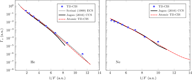
Figure 1: Static-field ionization rates $\Gamma_{s}$ for He and Ne. The rates computed with the current TD-CIS method are compared against the exact results of Scrinzi et al. [66] who used a full-dimensional complex scaling method, as well as Jagau [67] who used a complex-scaled coupled-cluster approach. Also shown are the TD-CIS results obtained with the specialization to spherical symmetry (see following article).

I.3 Time propagator

The EOMs (I–7) are solved by a simple 4^th order Runge–Kutta propagator, since that only requires the action of the Hamiltonian on the wavefunction. The action of the direct and exchange potentials on the particle orbitals $\ket*{\tilde{k}}$ is computed by solving Poisson’s problem via successive over-relaxation [68, 69]. The use of iterative solvers means that the computational complexity scales approximately linearly with the number of grid points, which in turn is given by

$$n_{g}=\kappa n_{x}n_{y}n_{z}n_{c},\quad\kappa=\begin{cases}1,&\textrm{spin-restricted},\\ 2,&\textrm{spin-unrestricted},\end{cases}$$

and $n_{c}$ is the number of channels. Orthogonality of the particle orbitals to the source orbitals is maintained by projecting out the latter from the former, every time the Hamiltonian is applied.

To suppress reflections from the boundary of the computational domain, we use the complex-absorbing potential (CAP) by Manolopoulos [70], with a design parameter $\delta=0.2$ leading to $<$1\text{\,}\mathrm{\char 37\relax}\text{/}$$ reflection for all momenta above $k_{\textrm{min}}=$1.5\text{\,}\mathrm{{a.u.}}\text{/}$$ The CAP then spans the last $4.37\text{\,}\mathrm{B}\mathrm{o}\mathrm{h}\mathrm{r}$ of the box in each direction. To avoid lowering the convergence order of the propagator, the CAP is multiplied by the time step and applied as a mask function, separately from the other terms in the Hamiltonian. The reason for this is that the convergence of the propagator relies on the fact that the EOMs obey the Dirac–Frenkel variational principle

$$\matrixelement{\variation{\Psi}}{\hat{H}-\mathrm{i}\partial_{t}}{\Psi}=0\implies\bra{\variation{\Psi}}\perp\bra{\Psi}.$$ (I–19)

If the EOMs are derived assuming a Hermitian $\hat{H}$, the presence of the CAP may result in the EOMs no longer obeying (I–19). Applying the CAP as a mask function circumvents the issue.

I.4 Results

We now outline the capabilities of our TD-CIS implementation using He, Ne, and a variety of small molecules: LiH, H2O, and C2H4. In all cases the GAMESS-US [71] electronic structure program was used to compute the initial restricted Hartree–Fock (RHF) molecular orbitals (MOs); since only the basis set and the corresponding expansion coefficients of the MOs are required as inputs for the TD-CIS computations, any electronic structure program may be used; all the required one- and two-electron matrix elements are then evaluated by a Gaussian integral package internal to the TD-CIS code. The aug-cc-pVTZ basis set was used for each system.

Except for the case of He, the TD-CIS computations were all carried out using continuum grids that extended from $-22.5\text{\,}\mathrm{B}\mathrm{o}\mathrm{h}\mathrm{r}22.5\text{\,}\mathrm{B}\mathrm{o}\mathrm{h}\mathrm{r}$ in all spatial directions with $$270$\times$270$\times$270$$ grid points, yielding a spatial step size of $h\approx$0.167\text{\,}\mathrm{B}\mathrm{o}\mathrm{h}\mathrm{r}$$. The time step in all cases was $\tau=$0.002\text{\,}\mathrm{{a.u.}}\text{/}$\approx$0.05\text{\,}\mathrm{as}\text{/}$$.

I.4.1 Atoms; helium and neon

In the case of helium, accurate static-field ionization rates are available in the literature. Scrinzi et al. [66], in particular, computed the He ionization rates using a full-dimensional treatment within the exterior complex scaling (ECS) methodology. Jagau [67] used a complex-scaled coupled-cluster approach, at various levels of theory for the field-free reference state. We use these rates as a benchmark to confirm the validity of our TD-CIS implementation. The spatial grid extends from $-15\text{\,}\mathrm{B}\mathrm{o}\mathrm{h}\mathrm{r}15\text{\,}\mathrm{B}\mathrm{o}\mathrm{h}\mathrm{r}$, in all spatial directions with $$180$\times$180$\times$180$$ grid points, yielding a spatial step size $h\approx$0.168\text{\,}\mathrm{B}\mathrm{o}\mathrm{h}\mathrm{r}$$.

In order to compute the static-field ionization rates within TD-CIS, a time-dependent computation is run with the system initialized in the neutral state. With a static field applied, the time-dependent population of the neutral, $\absolutevalue{c_{0}(t)}^{2}$, is monitored. After an initial turn-on transient has passed, the long-time behaviour of $\absolutevalue{c_{0}(t)}^{2}$ is fit to an exponential decay ($\sim e^{-\Gamma_{s}t}$) to extract the static-field ionization rate $\Gamma_{s}$. Figure 1 shows the TD-CIS ionization rates, which are in excellent agreement with those obtained by Scrinzi et al. [66], Jagau [67]. At lower intensities, our computational box is not sufficiently large enough to contain the tunnel exit (see the discussion for H2O below). The apparent ionization rates at these intensities are the upper bound to the true tunnelling rate.

I.4.2 Convergence

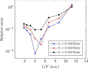
Figure 2: Relative errors of the He static field ionization rates shown in Figure 1 with respect to the atomic TD-CIS results, for various grid spacings.

As a test of the convergence of the calculations, we compute the static ionization rates for He for different grid spacings and time steps. We compare with the results from the atomic TD-CIS implementation, which is at the same level of theory and thus serves as our method limit. In figure 2, the convergence with respect to the grid spacing is shown. Its behaviour is non-uniform, reflecting the underlying complexity of the iterative algorithms. For the different time steps tried, i.e. $\tau\in\{0.001,0.002,0.004,0.008,0.016\}\;$\mathrm{{a.u.}}\text{/}$$, the change in the error was negligible for all field strengths $F$ and grid spacings $h$. The convergence with respect to the time step is most likely limited by the tolerance set for the Poisson solver employed for the Coulomb interaction.

I.4.3 LiH

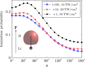
Figure 3: Angle-dependent half-cycle ionization yields for LiH for intensities of $10\text{\,}\mathrm{TW}\text{/}{\mathrm{cm}}^{2}$ (data scaled by $\times$100), $20\text{\,}\mathrm{TW}\text{/}{\mathrm{cm}}^{2}$ (data scaled by $\times$10), and $50\text{\,}\mathrm{TW}\text{/}{\mathrm{cm}}^{2}$. Here $\theta$ is the angle between the molecular axis and the electric field vector of the laser. We clearly see that doubling the intensity ($\sim F_{0}^{2}$) increased the ionization probability by more than one order of magnitude. The inset shows the ionizing orbital, along with the electric field vector $\mathbf{F}$ for the $\theta=$$$ configuration where the field points from the Li to the H atom.

The LiH molecule has two occupied orbitals in the RHF neutral ground state. However, due to the large binding potential of the HOMO$-1$ orbital, only the HOMO (highest occupied molecular orbital) orbital ionizes with non-negligible probability. Hence, we treat LiH as a single channel case, with the lower-lying RHF orbital frozen during the computations.

We calculate the half-cycle ionization yield using a smoothed half-cycle pulse defined as

$$F(t)=\begin{cases}0,&t<0,\\ F_{0}\sin^{2}(\alpha t),&0\leq t\leq t_{\textrm{max}},\\ 0,&t>t_{\textrm{max}},\end{cases}\quad\alpha\overset{\textrm{\tiny def}}{=}\frac{\omega_{L}}{\sqrt{2}},$$ (I–20)

where $t_{\textrm{max}}=\pi/\alpha$. This pulse shape mimics the high-intensity portion of a half-cycle of a laser field with frequency $\omega_{L}$, but using the smoothed half-cycle reduces artefacts that arise from an instantaneous turn-on had just a standard half-cycle field been used instead. For all remaining computations, we use $\omega_{L}=$0.057\text{\,}\mathrm{Ha}\text{/}$$, which corresponds to an $800\text{\,}\mathrm{nm}\text{/}$ laser field. In addition to minimizing the computational load required to compute the ionization compared to that needed for a multi-cycle pulse, using a half-cycle-type pulse allows us to see the orientation-dependence of the ionization yields when ionizing polar molecules like LiH (and H2O considered below).

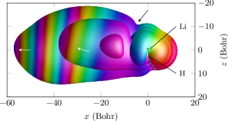
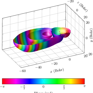
Figure 4: Continuum electron wave packet after the end of the pulse [$t=t_{\textrm{max}}$ in (I–20)], for $\theta=$$$, and $20\text{\,}\mathrm{TW}\text{/}{\mathrm{cm}}^{2}$.

The angle dependent half-cycle ionization yields are presented in Figure 3 for the laser intensities for a variety of laser intensities. The inset shows the definition of the angle between the molecular axis and the electric field of the ionizing pulse; $\theta=$$$ corresponds to the electric field vector of the laser pointing from the Li to the H atom. Since the motion of the liberated electron will be opposite to the direction of the electric field, the angle corresponding to the peak of the angle-dependent ionization ($\theta\approx$$-$$$) sees the liberated electron escape from the initial HOMO orbital (located on the H atom) across the Li atom.

Figure 4 shows the continuum electron wave packet at the end of the laser pulse, for the case of $\theta=$$$, i.e the laser field is perpendicular to the molecular axis. The tunnel barrier is clearly visible around $x\approx$-5\text{\,}\mathrm{B}\mathrm{o}\mathrm{h}\mathrm{r}$$, in that the wave packet appears “pinched” (marked with a black arrow). The colour map which corresponds to the phase indicates that the wavefront (and hence the direction of travel) right after the tunnel exit is directed upwards (smaller value of $\theta$), but after some distance, the electron motion tends to $-90\mathrm{°}$, i.e parallel to $-x$, opposite to the field polarization (marked with white arrows). This agrees with the observation above that the electron preferentially escapes the potential in the vicinity of the Li atom.

I.4.4 H2O

Due to the lower symmetry of H2O, belonging to the $C_{2\mathrm{v}}$ point group, it is not enough to compute the photoionization yields as a function of $\theta$ only. We therefore choose a 9th-order Lebedev grid [72] that can represent integrals involving spherical harmonics up to $\ell=\left\lfloor\frac{9-1}{2}\right\rfloor=4$ exactly. From this grid of 38 field orientations, only 16 that are unique with respect to the $C_{2\mathrm{v}}$ symmetry are actually computed, and then replicated. The resulting yield surface is then transformed to the equivalent expansion in spherical harmonics; the results are shown in Figure 5. For the three highest occupied molecular orbitals and four different intensities of the driving field, the ionization yields are plotted as a function of the angles $\theta$ and $\phi$, as well as angle-integrated. The same field (I–20) is used as for LiH, i.e a half-cycle of $800\text{\,}\mathrm{nm}\text{/}$. Additionally, static ionization rates are computed (similarly to He and Ne) orthogonal to the molecular plane, i.e along the lobes of the HOMO (the $x$ axis), and compared with the CCS results of Jagau [73].

The dynamic photoionization yields can be compared to tunnelling yields estimated from a Keldysh-like [74] formula for the ionization rate:

$$w \sim\exp\left[-\frac{1}{3\tilde{\mathcal{E}}}g(\gamma)\right],$$ (I–21)

$$g(\gamma) \overset{\textrm{\tiny def}}{=}\frac{3}{2\gamma}\left[\left(1+\frac{1}{2\gamma^{2}}\right)\operatorname{arcsinh}\gamma-\frac{\sqrt{1+\gamma^{2}}}{2\gamma}\right],$$

where $\gamma\overset{\textrm{\tiny def}}{=}\sqrt{I_{\mathrm{p}}/2U_{\mathrm{p}}}$, $\tilde{\mathcal{E}}\overset{\textrm{\tiny def}}{=}F[2(2I_{\mathrm{p}})^{3/2}]^{-1}$, and the estimated ionization yield $y=wt_{\textrm{max}}$. We attribute the deviations of the predictions by the tunnelling formula from the TD-CIS results to the neglect of many-electron dynamics in the molecule in (I–21).

Table 1: Tunnel exit (I–22) for H2O; missing values indicate barrier suppression. The MO energies are given in the second row. The CAP starts at $18.13\text{\,}\mathrm{B}\mathrm{o}\mathrm{h}\mathrm{r}$.

Intensity	$F$	HOMO	HOMO$-1$	HOMO$-2$
($\mathrm{TW}\text{/}{\mathrm{cm}}^{2}$)	($\mathrm{{a.u.}}\text{/}$)	$0.511\text{\,}\mathrm{H}\mathrm{a}$	$0.585\text{\,}\mathrm{H}\mathrm{a}$	$0.723\text{\,}\mathrm{H}\mathrm{a}$
$400$	$0.107$
$200$	$0.075$			$6.733$
$100$	$0.053$	$6.727$	$8.328$	$11.106$
$50$	$0.038$	$11.100$	$13.141$	$16.887$

The non-exponential behaviour of the HOMO$-2$ yield for the smallest intensity is an artefact of limited computational box size. We compute the classical tunnel exit according to

$$r_{\textrm{exit}}=\frac{2I_{\mathrm{p}}missing}{4F}+\sqrt{\left(\frac{2I_{\mathrm{p}}missing}{4F}\right)^{2}-\frac{2I_{\mathrm{p}}missing}{F}},$$ (I–22)

where $I_{\mathrm{p}}$ is the magnitude of the orbital energy in Koopman’s approximation, and $F=\sqrt{I}$ the peak amplitude of the ionizing field. Table 1 shows the estimated tunnel exits for the three highest occupied molecular orbitals and the various field strengths. For the weakest field, we see that the tunnel exit of HOMO$-2$ is very close to the onset of the CAP. This means that in that particular channel, Rydberg states (which extend into the classically forbidden region in the tunnel but not beyond it) incorrectly count towards the photoionization yield, since we compute ionization as loss of norm. Hence, what we observe is rather a polarization effect, than true ionization, for these MOs. Also the angular distribution of the yield for HOMO$-2$ is affected by this artefact, resulting in a qualitatively different shape for the lowest intensity. This error decreases with increased box size, at the cost of longer computation times.

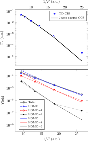
Figure 5: Top panel: Static ionization rates of H2O, orthogonal to the molecular plane, compared with the CCS results of Jagau [73]. Bottom panel: Half-cycle intensity-dependent photoioniziation yield of H2O, total, as well as resolved on the RHF orbitals. The “knee” observed at lower intensities for HOMO$-2$ is a polarization effect (see main text). For comparison, the solid lines indicate the ionization yields as predicted by an Keldysh-like theory (I–21), where only the exponential factor due to the ionization potential of the molecular orbitals, and the field strength is considered. These lines have been normalized to the respective TD-CIS results at $100\text{\,}\mathrm{TW}\text{/}{\mathrm{cm}}^{2}$.

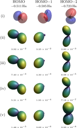
Figure 6: (i) RHF orbitals of H2O, along with their angle-resolved ionization yields, for the following intensities: (ii) $400\text{\,}\mathrm{TW}\text{/}{\mathrm{cm}}^{2}$, (iii) $200\text{\,}\mathrm{TW}\text{/}{\mathrm{cm}}^{2}$, (iv) $100\text{\,}\mathrm{TW}\text{/}{\mathrm{cm}}^{2}$, (v) $50\text{\,}\mathrm{TW}\text{/}{\mathrm{cm}}^{2}$. The yields have been normalized to their respective maximum values, indicated below each distribution.

Table 2: Overlaps between the molecular orbitals of the H2O ground state and those of the O ground state. We see that to a very large degree, the MOs of H2O are atomistic.

	O $\mathrm{p}_{x}$	O $\mathrm{p}_{y}$	O $\mathrm{p}_{z}$
H2O HOMO	$0.995$	$0.000$	$0.000$
H2O HOMO$-1$	$0.000$	$0.000$	$0.951$
H2O HOMO$-2$	$0.000$	$0.944$	$0.000$

We now turn to the angular distributions of the photoionization yields; as we can see in the first row of Figure 6, the molecular orbitals (MOs) are very similar to atomic orbitals (AOs) of $\mathrm{p}$ symmetry. The small deviation of the MOs from pure spherical symmetry leads however to drastically different angularly resolved ionization yields, where the electron preferentially leaves the molecule over the O atom, which we attribute primarily to dipole effects. This pattern persists for all intensities, although the HOMO$-1$ contribution in the direction of the two H atoms does seem to increase slightly with intensity [middle column of row (ii) in Figure 6]. The nodal planes in the HOMO and HOMO$-2$ yields are mandated by the $C_{2\mathrm{v}}$ symmetry. The observed nodal plane in the HOMO$-1$ yields is however required by an approximate, higher symmetry, $D_{2\mathrm{h}}$. This serves to further highlight the atomistic nature of the H2O MOs, which we can quantitatively investigate by computing their overlaps with the $\mathrm{p}$ AOs of O; see Table 2.

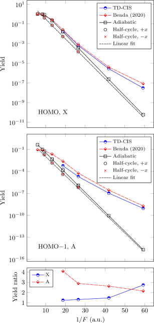
Figure 7: H2O yields for ionization from the two highest-lying occupied orbitals using an eight-cycle pulse, as a function of inverse field strength. The yields are compared with the results of Benda et al. [75], as well as with an adiabatic estimate (I–23) formed from the half-cycle yields presented in Figure 5. The bottom panel shows the ratio between the results of Benda et al. [75] and the present work.

In Figure 7, the photoionization yields along $x$ for an eight-cycle pulse with a $\sin^{2}$ envelope, and a carrier wavelength of $800\text{\,}\mathrm{nm}\text{/}$ are shown. The yields are compared with the results of Benda et al. [75] (specifically their coupled model B), and show very good agreement. The discrepancy can be mostly attributed to the difference in ionization potentials; in the present work, the MOs are slightly more bound than in the calculations by Benda et al. [75] ($13.90\text{\,}\mathrm{eV}\text{/}$ vs. $13.15\text{\,}\mathrm{eV}\text{/}$ for HOMO, and $15.92\text{\,}\mathrm{eV}\text{/}$ vs. $15.15\text{\,}\mathrm{eV}\text{/}$ for HOMO$-1$), which has a strong effect due to the exponential sensitivity of strong-field ionization to the ionization potential.

Also shown are the half-cycle yields $y_{n}$ in the lower panel of Figure 5, along with their logarithms $\log_{10}(y_{i})$ appear to follow a linear trend as a function of the inverse field strength $1/F_{n}$. We may therefore estimate the eight-cycle yield adiabatically as

$$y =1-\exp\left\{-\int_{-\infty}^{\infty}\mathrm{d}t\;\Gamma[F(t)]\right\}$$ (I–23)

$$\approx 1-\exp\left[-\sum_{i}\langle\Gamma(F_{i})\rangle\right]=1-\prod_{i}[1-\tilde{y}(F_{i})],$$

where $F_{i}$ is the peak field amplitude of the $i$:th half-cycle, and the corresponding yields $\tilde{y}(F_{i})$ are found using an linear fit to the half-cycle yields $y_{n}$. This estimate of course neglects any cycle-to-cycle effects, which explains its deviation from the true eight-cycle results at lower intensities (higher $1/F$). For higher intensities, the adiabatic results are however in good agreement with the full calculations.

I.4.5 C2H4

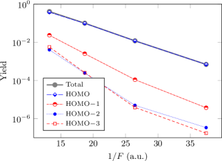
Figure 8: Intensity-dependent photoioniziation yield of C2H4, total as well as resolved on the RHF orbitals.

Ionization yields are computed similarly to H2O, as detailed above, but C2H4 belonging to the $D_{2\mathrm{h}}$ point group, has higher symmetry than H2O, and only 9 unique field orientations are required. The results are shown in Figure 8, and the corresponding angular distributions in Figure 9.

Table 3: Tunnel exit (I–22) for C2H4; missing values indicate barrier suppression. The MO energies are given in the second row. The CAP starts at $18.13\text{\,}\mathrm{B}\mathrm{o}\mathrm{h}\mathrm{r}$.

Intensity	$F$	HOMO	HOMO$-1$	HOMO$-2$	HOMO$-3$
($\mathrm{TW}\text{/}{\mathrm{cm}}^{2}$)	($\mathrm{{a.u.}}\text{/}$)	$0.381\text{\,}\mathrm{H}\mathrm{a}$	$0.507\text{\,}\mathrm{H}\mathrm{a}$	$0.593\text{\,}\mathrm{H}\mathrm{a}$	$0.648\text{\,}\mathrm{H}\mathrm{a}$
$200$	$0.075$				$5.412$
$100$	$0.053$		$6.636$	$8.494$	$9.615$
$50$	$0.038$	$7.347$	$10.988$	$13.360$	$14.858$
$25$	$0.027$	$11.871$	$16.726$	$19.997$	$22.081$

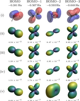
Figure 9: (i) RHF orbitals of C2H4, along with their angle-resolved ionization yields, for the following intensities: (ii) $200\text{\,}\mathrm{TW}\text{/}{\mathrm{cm}}^{2}$, (iii) $100\text{\,}\mathrm{TW}\text{/}{\mathrm{cm}}^{2}$, (iv) $50\text{\,}\mathrm{TW}\text{/}{\mathrm{cm}}^{2}$, (v) $25\text{\,}\mathrm{TW}\text{/}{\mathrm{cm}}^{2}$. The yields have been normalized to their respective maximum values, indicated below each distribution.

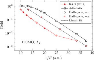
Figure 10: C2H4 adiabatic dynamic yields (I–23) for a seven-cycle pulse, compared with the results of Krause and Schlegel [18].

Again, as in the case of H2O, we find that for the lower intensities, the yields for HOMO$-\{2,3\}$ deviate from the expected exponential behaviour, with a “knee” observed in the integrated ionization yield, and qualitatively different angular distributions [row (v) in Figure 9], whereas HOMO and HOMO$-1$ follow their respective trends also for the lowest intensity. Table 3 lists the tunnel exits for the various MOs and intensities, and for HOMO$-\{2,3\}$ and the lowest intensity, these are well beyond the CAP onset, implying we are measuring mainly a polarization effect.

In Figure 10 we compare an adiabatic estimation according to (I–23) of the seven-cycle yield with the results by Krause and Schlegel [18]. Their quoted ionization rates were multiplied by the duration of the pulse [cf. their equation (8)] to obtain the yields; we do not find agreement between the different calculations. Extracting the true ionization rates is non-trivial, due to the temporal intensity averaging, which is why we cannot easily compare directly with the half-cycle yields presented in Figure 8. We also note the experimental work of Talebpour et al. [76], the comparison with which would require detailed knowledge of the experimental conditions, not available to us, as well as extensive simulations.

I.5 Conclusions

We have described an implementation of TD-CIS for small gas-phase molecules, with the continuum electron resolved on a Cartesian grid, which allows an accurate description of the photoelectron in strong-field processes. We applied this method to a few molecules, finding reasonable results for the angularly resolved ionization probability. An implementation of t+iSURF for TD-CIS in the atomic case is presented in the following article [1], and for the general case an implementation is underway, which would allow us to efficiently compute photoelectron spectra for various processes of interest.