Exact Master Equation for Quantum Brownian Motion with Generalization to Momentum-Dependent System-Environment Couplings

Abstract

In this paper, we generalize the quantum Brownian motion to include momentum-dependent system-environment couplings. The resulting Hamiltonian is given by $H_{\textsl{tot}}=\hbar\omega_{\textsc{s}}a^{\dagger}a+\sum_{k}\hbar\omega_{k}b_{k}^{\dagger}b_{k}+\sum_{k}\hbar(V_{k}a^{\dagger}b_{k}+V_{k}^{*}b_{k}^{\dagger}a)+\sum_{k}\hbar(W_{k}a^{\dagger}b_{k}^{\dagger}+W_{k}^{*}b_{k}a)$. The conventional QBM model corresponds to the spacial case $W_{k}=V_{k}$. The generalized QBM is more complicated but the generalization is necessary. This is because the particle transition and the pair production between the system and the environment represent two very different physical processes, and usually cannot have the same coupling strengths. Thus, the conventional QBM model, which is well-defined at classical level, is hardly realized in real quantum physical world. We discuss the physical realizations of the generalized QBM in different physical systems, and derive its exact master equation for both the initial decoupled states and initial correlated states. The Hu-Paz-Zhang master equation of the conventional QBM model is reproduced as a special case. We find that the renormalized Brownian particle Hamiltonian after traced out all the environmental states induced naturally a momentum-dependent potential, which also shows the necessity of including the momentum-dependent coupling in the QBM Hamiltonian. In the Hu-Paz-Zhang master equation, such a renormalized potential is misplaced so that the correct renormalization Hamiltonian has not been found. With the exact master equation for both the initial decoupled and and initial correlated states, the issues about the initial jolt which is a long-stand problem in the Hu-Paz-Zhang master equation is also re-examined. We find that the so-called “initial jolt”, which has been thought to be an artificial effect due to the use of the initial decoupled system-environment states, has nothing do to with the initial decoupled state. The new exact master equation for the generalized QBM also has the potential applications to photonics quantum computing.

I Introduction

As it is well-known, any realistic system inevitably interacts with its environment. For nano-scale quantum devices or more general mesoscopic and quantum systems, such interactions are usually not negligible, and thus these systems must be treated as open quantum systems. The essential physics of open quantum systems is the entanglement generation between the system and the environment so that the system cannot be retained in pure quantum states. This makes the system lose its quantum coherence, known as quantum decoherence which is the key obstacle in the development of quantum technology. Up to date, theoretical description of open quantum systems is still a big challenge in both fundamental research and practical applications. The major difficulty for solving the dynamics of open quantum systems is how to find the physically reasonable system-environment coupling which is usually unknown in priori, and how to derive unambiguously the equation of motion, called the master equation, for the dynamical evolution of open quantum systems in terms of the reduced density matrix which is not always computable.

Historically, a prototype of open quantum systems is the quantum Brownian motion (QBM) Grabert1988 ; Weiss1992 . Quantum mechanically, the Brownian particle is modeled as a harmonic oscillator that linearly couples to the environment which is made of a continuous distribution of infinite number of harmonic oscillators, as originally proposed in the seminal works of Feynman and Vernon Feynman1963 and also Caldeira and Laggett Leggett1983a ; Leggett1983b . The system-environment coupling in QBM was assumed as a strict linear coupling $\sum_{k}\!C_{k}xq_{k}$, where $x$ and $q_{k}$ are the position coordinates of the system and environment oscillators, respectively, and $C_{k}$ is the coupling amplitude. The exact master equation of the QBM for such a system-environment coupling has been derived during 1980’s $\sim$ 1990’s with different approaches Leggett1983a ; Haake1985 ; Hu1992 ; Karrlein1997 . Correspondingly, the dissipative dynamics of QBM has been extensively investigated in a rather broad physical research areas Grabert1988 ; Weiss1992 . In particular, the classical dissipative dynamics, the fluctuation-dissipation theorem and the classical Langenvin equation have been deduced from this quantum Brownian motion in the weak-coupling and high temperature limits Grabert1988 ; Weiss1992 ; Feynman1963 ; Leggett1983a ; Leggett1983b .

Microscopically, the above classically well-defined linear coupling $\sum_{k}\!C_{k}xq_{k}$ depicts the Brownian particle dissipation and fluctuations through energy exchange between the system and the environment. However, probably one does not realize that this system-environment coupling is physically not self-consistent at quantum level. Specifically, the Hamiltonian of a harmonic oscillator can be written as $H_{\textsc{s}}=\hbar\omega_{\textsc{s}}a^{\dagger}a$, where $\hbar\omega_{\textsc{s}}$ is the quanta of the harmonic oscillator energy of the system, and $a^{\dagger}$ and $a$ are the corresponding creation and annihilation operators obeying commutation relation $[a,a^{\dagger}]=1$. Similarly, the Hamiltonian of the environment made by infinite number of harmonic oscillators can be expressed as $H_{\textsc{e}}=\sum_{k}\hbar\omega_{k}b_{k}^{\dagger}b_{k}$, where $b_{k}^{\dagger}$, $b_{k}$ are the creation and annihilation operators of the quantum oscillator mode $k$ with frequency $\omega_{k}$. Consequently, the linear system-environment coupling Hamiltonian can be expressed as $\sum_{k}\!C_{k}xq_{k}=\sum_{k}\!\hbar V_{k}(a^{\dagger}b_{k}+b_{k}^{\dagger}a+a^{\dagger}b_{k}^{\dagger}+b_{k}a)$ with $V_{k}=C_{k}/2\sqrt{Mm_{k}\omega_{\textsc{s}}\omega_{k}}$, where $M$, $m_{k}$ are the masses of the system oscillator and the environmental oscillator mode $k$. It shows that the first two terms, proportional to $a^{\dagger}b_{k}+b_{k}^{\dagger}a$, depict the energy exchange (energy transition) between the system and the environment. While the last two terms, proportional to $a^{\dagger}b_{k}^{\dagger}+b_{k}a$, describe the processes of generating and annihilating separately two quanta of energy out of the blue, from nothing. As one knows, the energy quanta of harmonic oscillator can be realized with photons or phonons, and physically one can generate or annihilate two photons (phonons) through non-linear crystals or atomic virtual states, but these physical processes are very different from the single photon transition processes of the first two terms in linear quantum optics. In other words, in reality, the coupling strength $V_{k}$ for the single particle transition processes is usually not the same as that of the two particle generation or annihilation.

Analogy to the above linear coupling between the system and the environment for the QBM, a similar situation also occurs in the canonical quantization of light-matter interaction. In quantum optics, under the dipole momentum approximation, the interesting light-matter interaction is mainly determined by $-\bm{d}\cdot\bm{E}(x,t)$, where $\bm{d}=q\bm{r}$ is the atomic dipole moment and $\bm{E}(x,t)$ is the radiative electric field. Treating approximately the atom as a two-level system, the above light-matter interaction can be written quantum mechanically as $-\bm{d}\cdot\bm{E}(x,t)=\sum_{k}g_{k}\sigma^{x}(b_{k}+b_{k}^{\dagger})=\sum_{k}g_{k}(\sigma^{+}b_{k}+\sigma^{-}b_{k}^{\dagger}+\sigma^{+}b_{k}^{\dagger}+\sigma^{-}b_{k})$, where $\sigma^{x}=\sigma^{-}+\sigma^{+}$ is the Pauli matrix, and $b_{k}^{\dagger}$, $b_{k}$ are the creation and annihilation operators of photons for the radiative field mode $k$. In this light-matter interaction, the first two terms proportional to $\sigma^{+}b_{k}+\sigma^{-}b_{k}^{\dagger}$ depict the electron transitions in atoms from the low-energy state to the high-energy state by absorbing a photon, and from the high-energy state back to the low-energy state by emitting a photon. These are the fundamental physical processes for light-matter interaction. While, there are other two terms, proportional to $\sigma^{+}b_{k}^{\dagger}+\sigma^{-}b_{k}$, which describe the electron transitions from the low-energy state to the high-energy state by emitting a photon, and from the high-energy state to the low-energy state by absorbing a photon. Actually, the last two processes barely occur due to the law of energy conservation, see Fig. 1, also see more discussions given in the next section.

In the literature, these physically infeasible processes in the linear coupling of the QBM and in the light-matter interaction of quantum optics are often called the counter-rotating terms. They can usually be eliminated under the so-called rotating wave approximation. In the high-temperature and weak-coupling limit, it can be shown that the contributions from these counter-rotating terms are negligible. However, in the strong coupling and low temperature regime, the counter-rotating terms could make a significant effect. In recent years, many effects have been devoted to search the counter-rotating effects theoretically and also experimentally Zheng2008 ; Niemczyk2010 ; Li2013 ; Garziano2016 ; Xu2016 ; Wang2017 ; Yoshihara2017 . Here we should point out that these counter-rotating terms either are forbidden by the energy conservation law for every individual microscopic physical processes, or can be modified by the comprehensive physical description of the system-environment couplings. Specifically, for an example, for the radiative electromagnetic field, $\bm{E}=-\partial\bm{A}/\partial t$ and $\bm{B}=\nabla\times\bm{A}$ where the vector potential $\bm{A}$ and the electric field $\bm{E}$ are the generalized coordinate and momentum in quantum electrodynamics (QED). Besides the atomic dipole moment interaction with the electric field, there is also the atomic magnetic dipole moment interaction with the magnetic field. Both interactions come from the position-momentum dependent atom-light interaction $-\frac{q}{m}\bm{A}\cdot\bm{P}_{\textsl{e}}$, where $\bm{P}_{\textsl{e}}$ is the electron momentum Tannoudji1998 . For the QBM, besides the linear coupling between the oscillator coordinates of the system and the environment, there are also the momentum-dependent system-environment couplings. When these contributions are elaborated, the inconsistent processes in system-environment couplings of open quantum systems can be diminished.

In this paper, we shall provide first a detailed analysis of the system-environment couplings for open quantum systems in general, and then generalize the QBM by including the momentum-dependent coupling to get rid of the possible ambiguity of system-environment couplings at quantum level. We shall also discuss practical realizations of such a generalization. In Sec. III, we will derive the exact master equation of the generalized QBM for both the initial decoupled and initial correlated states. We shall also explore the relation of dissipation and fluctuation dynamics in open quantum systems with the decay and diffusions of the Brownian particle. In Sec. IV, we will show how the previous Hu-Paz-Zhang master equation for the QBM without including momentum-dependent coupling Leggett1983a ; Haake1985 ; Hu1992 ; Karrlein1997 can be reproduced as a very special case. We will also re-examine some long-standing debated issues about QBM, such as the origin of the initial jolt phenomena and the initial decoupled state problem one often questioned for the study of the QBM with the exact master equation. Finally, discussions and perspectives are given in Sec. V. In Appendix A, the nonequilibrium Green functions for open quantum systems we previously introduced are generalized to open systems containing pairing couplings through the Heisenberg equation of motion. The generalized nonequilibrium fluctuation-dissipation theorem in the time-domain is also derived there.

II A General Analysis of Momentum-Dependent System-Environment Couplings

In the early studies of quantum dissipative dynamics, system-environment couplings in open systems are mainly modeled based on classical mechanics. The prototype example is given in the pioneering work by Feynman and Vernon for developing their influence functional theory for QBM Feynman1963 . In the exploration of the dissipative and noise effects of other interaction systems on the system of interest, Feynman and Vernon proposed a general test system $x$ interacting to linear systems $\{q_{k}\}$ (an oscillator bath) with the Lagrangian

$$L_{\text{FV}}\!\!=\!L_{\textsc{s}}(\dot{x},x)\!+\!\frac{1}{2}\sum_{k}\!m_{k}(\dot{q}_{k}^{2}\!-\!\omega_{k}^{2}q_{k}^{2})\!-\!U(x)\!\sum_{k}\!C_{k}q_{k}.$$ (1)

Without loss of generality, one usually takes a linear coupling $U(x)=x$. The oscillator bath is an environment consisting of a collection of harmonic oscillators with a continuous frequency distribution. Such an environment can be easily realized as radiative electromagnetic fields or vibrations of lattices in matter. The Lagrangian formulation in terms of the dynamical variables of positions and velocities is setup in order to conventionally use the Feynman’s path integrals for the trace over all the environmental states Feynman1965 . In such circumstances, the path integrals over environmental degrees of freedom can be done exactly. Thus the environment effect on the test system is given by an influence functional of coordinates of the system only. It is equivalent to external semiclassical dissipative and fluctuating (random) forces acting on the test system. As Feynman and Vernon pointed out Feynman1963 , if a general non-linear interaction system $q_{k}$ is weakly coupled to a test system $x$ with a more general interaction potential $U(x)U^{\prime}(\{q_{k}\})$ which is small, then the effect on the test system is that of a sum of oscillators whose frequencies correspond to the possible transitions of the interaction system. Thus, to the extent that second order perturbation theory yields sufficient accuracy, the effect of an interaction system is that of a linear system Feynman1963 .

In 1980’s, Caldeira and Leggett made further investigations to QBM and quantum tunneling of dissipative systems, in which similar linear couplings are made in order to derive a dissipative (damping) equations of motion from quantum mechanics Leggett1983a ; Leggett1983b . Specifically, to consistently produce the semiclassical damped equation of motion, $M\ddot{x}+\eta(x)\dot{x}+\mathrm{d}V/\mathrm{d}x=F_{\textsl{ext}}(t)$ where $F_{\textsl{ext}}(t)$ is an external force, Caldeira and Leggett also proposed the environment as a continuous frequency distribution of a set of harmonic oscillators interacting linearly with the system,

$$L_{\text{CL}}={} \frac{1}{2}M\dot{x}^{2}\!-\!V(x)\!+\!\frac{1}{2}\sum_{k}m_{k}(\dot{q}_{k}^{2}\!-\!\omega_{k}^{2}q_{k}^{2})$$

$$\!-\!\sum_{k}F_{k}(x)q_{k}\!-\!\sum_{k}F_{k}^{2}(x)/2m_{k}\omega_{k}^{2}.$$ (2)

When the system is a tunneling system, Eq. (2) is often called the Caldeira–Leggett model in the literature. Except for the last term which is added as a counter-term for the stability of potential renormalization, Eq. (2) is equivalent to Eq. (1). For $x$-independent dissipation $\eta(x)=\eta$, the semiclassical damped equation of motion can be realized with the strict linear coupling between the system and the environment $F_{k}(x)=C_{k}x$. Other more complicated coupling mechanisms are analyzed extensively in the Appendix C of Leggett1983b but these analysis are indeed superfluous from the microscopical level of interacting systems, as Caldeira and Leggett pointed out in their own work Leggett1983b .

To have a clear physical picture on the microscopical level of interacting systems in the Feynman–Vernon model or the Caldeira–Leggett model, it will be more convenient to reformulate the Hamiltonian of Eq. (2) in the second quantization framework:

$$H_{\text{CL}}={} \frac{p^{2}}{2M}\!+\!V(x)\!+\!\sum_{k}\Bigl{(}\frac{p_{k}^{2}}{2m_{k}}+\frac{1}{2}m_{k}\omega_{k}^{2}q_{k}^{2}\Bigr{)}$$

$$+\!\sum_{k}F_{k}(x)q_{k}\!+\!\sum_{k}F_{k}^{2}(x)/2m_{k}\omega_{k}^{2}$$

$$={} \sum_{i}\varepsilon_{i}a_{i}^{\dagger}a_{i}\!+\!\!\sum_{k}\hbar\omega_{k}b_{k}^{\dagger}b_{k}\!+\!\!\sum_{ijk}V_{ijk}a_{i}^{\dagger}a_{j}(b_{k}^{\dagger}+b_{k}).$$ (3)

Here, $\varepsilon_{i}$ is the spectrum of the system Hamiltonian $H_{\textsc{s}}=\frac{1}{2M}p^{2}+V_{\textsl{eff}}(x)$ with $H_{\textsc{s}}\lvert\psi_{i}\rangle=\varepsilon_{i}\lvert\psi_{i}\rangle$, where $V_{\textsl{eff}}(x)=V(x)+\sum_{k}\frac{F_{k}^{2}(x)}{2m_{k}\omega_{k}^{2}}$. The operators $a_{i}^{\dagger}$ and $a_{i}$ are respectively the creation and annihilation operators that create the system state $\lvert\psi_{i}\rangle$ from the vacuum state $\lvert 0\rangle$: $a_{i}^{\dagger}\lvert 0\rangle=\lvert\psi_{i}\rangle$ and $a_{i}\lvert 0\rangle=0$. These creation and annihilation operators obey the commutation or anti-commutation relation, $[a_{i},a_{j}^{\dagger}]_{\mp}=a_{i}a_{j}^{\dagger}\mp a_{j}^{\dagger}a_{i}=\delta_{ij}$, depending on the system being a bosonic or a fermionic system. The creation and annihilation operators $b_{k}^{\dagger}$, $b_{k}$ of the harmonic bath can also be defined by $b_{k}^{\dagger}=\sqrt{\frac{m_{k}\omega_{k}}{2\hbar}}(q_{k}-\frac{i}{m_{k}\omega_{k}}p_{k})$, $b_{k}=\sqrt{\frac{m_{k}\omega_{k}}{2\hbar}}(q_{k}+\frac{i}{m_{k}\omega_{k}}p_{k})$. The system-environment coupling $V_{ijk}=\sqrt{\frac{\hbar}{2m_{k}\omega_{k}}}\langle\psi_{i}\rvert F_{k}(x)\lvert\psi_{j}\rangle$ describes the transition of the system from the state $\lvert\psi_{j}\rangle$ to the state $\lvert\psi_{i}\rangle$ due to the linear coupling to the environmental oscillating mode $\omega_{k}$. Now one can see a physically troublesome process depicted by the linear system-environment coupling in the Feynman–Vernon model and the Caldeira–Leggett model. That is, the system emits or absorbs a “photon” with the same energy results in the same transition of the system from the state $\lvert\psi_{j}\rangle$ to the state $\lvert\psi_{i}\rangle$. This is quantum mechanically infeasible, as shown in Fig. 1. This seems to indicate that Eqs. (1) and (2) are at least incomplete at quantum level if it is not unphyscial.

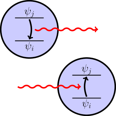
(a)  feasible processes

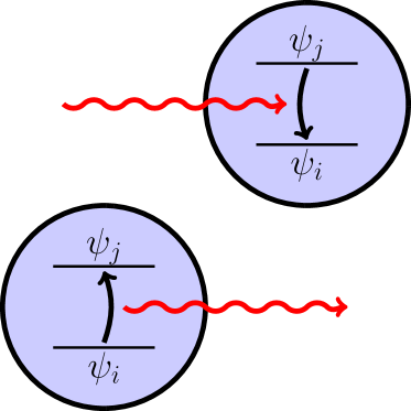
(b)  infeasible processes

Figure 1: A microscopic picture of the momentum-independent couplings between the system and the environment in Eq. (3). (a) The process of a particle decay from the high energy state $\lvert\psi_{j}\rangle$ to the low energy state $\lvert\psi_{i}\rangle$ by emitting an energy quanta described by the term $V_{ijk}a_{i}^{\dagger}a_{j}b_{k}^{\dagger}$, and its Hermitian conjugation process; (b) The process of the particle decay from the high energy state $\lvert\psi_{j}\rangle$ to the low energy state $\lvert\psi_{i}\rangle$ by absorbing an energy quanta described by the term $V_{ijk}a_{i}^{\dagger}a_{j}b_{k}$, and its Hermitian conjugation process, which are physically infeasible.

In fact, a general Hamiltonian of the system coupled to the oscillator-bath environment should contain both the position-dependent and the momentum-dependent system-environment couplings, as Caldeira and Leggett pointed out in their original paper Leggett1983b ,

$$H_{\textsc{s-e}}={} \frac{p^{2}}{2M}\!+\!V(x)\!+\!\sum_{k}\Bigl{(}\frac{p_{k}^{2}}{2m_{k}}+\frac{1}{2}m_{k}\omega_{k}^{2}q_{k}^{2}\Bigr{)}$$

$$+\!\sum_{k}\bigl{[}F_{k}(p,x)q_{k}+G_{k}(p,x)p_{k}\bigr{]}\!+\!\Phi(p,x),$$ (4)

where $\Phi(p,x)$ is a counter-term for the renormalization of system Hamiltonian arisen from the system-environment couplings. Equation (4) contains various position and momentum dependent system-environment couplings. The second quantization form of the above Hamiltonian is given by

$$H_{\textsc{s-e}}={} \!\sum_{i}\varepsilon_{i}a_{i}^{\dagger}a_{i}\!+\!\sum_{k}\hbar\omega_{k}b_{k}^{\dagger}b_{k}$$

$$+\!\sum_{ijk}\bigl{(}V_{ijk}^{\prime}a_{i}^{\dagger}a_{j}b_{k}^{\dagger}+V_{ijk}^{\prime*}a_{j}^{\dagger}a_{i}b_{k}\bigr{)}.$$ (5)

Similarly, $\varepsilon_{i}$ is the spectrum of the system Hamiltonian $H_{\textsc{s}}=\frac{p^{2}}{2M}+V(x)+\Phi(p,x)$ with $H_{\textsc{s}}\lvert\psi_{i}\rangle=\varepsilon_{i}\lvert\psi_{i}\rangle$, the system-environment couplings $V_{ijk}^{\prime}$ are given by

$$V_{ijk}^{\prime}={} \sqrt{\frac{\hbar}{2m_{k}\omega_{k}}}\langle\psi_{i}\rvert F_{k}(p,x)\lvert\psi_{j}\rangle$$

$$\qquad\qquad+i\sqrt{\frac{\hbar m_{k}\omega_{k}}{2}}\langle\psi_{i}\rvert G_{k}(p,x)\lvert\psi_{j}\rangle.$$ (6a)

Now it shows that the system-environment coupling (the last two terms in Eq. (5)) contains the physical process of the system transiting from the state $\lvert\psi_{j}\rangle$ to the state $\lvert\psi_{i}\rangle$ by emitting a photon, and the inverse process of transiting the state $\lvert\psi_{i}\rangle$ back to the state $\lvert\psi_{j}\rangle$ by absorbing a photon with the same energy. In other words, the original ambiguity in the Feynman-Vernon model and in the Caldeira-Leggett model can be diminished when a momentum-dependent system-reservoir coupling co-exists.

The above analysis indicates that although Eqs. (1) and (2) are well-defined in classical mechanics, their quantum mechanical version is somehow inconsistent and contains some physically infeasible processes. But the inconsistency can be eliminated when a momentum-dependent system-environment coupling is included, as it is shown above. In fact, for atoms interacting with radiative electromagnetic field, the momentum-dependent coupling is naturally manifested. Explicitly, the non-relativistic atom-photon interaction Hamiltonian can be rigorously written as Tannoudji1998

$$H_{\textsl{e-p}}=\!\sum_{i}\frac{1}{2m}\bigl{[}\bm{P}_{i}\!-\!e\bm{A}(\bm{r}_{i})\bigr{]}^{2}\!\!+\!\sum_{\mathclap{\bm{k},\lambda=1,2}}\hbar\omega_{\bm{k}}b_{\bm{k},\lambda}^{\dagger}b_{\bm{k},\lambda}\!+\!V_{\textsl{coul}},$$ (7)

where $m$ and $e$ are the electron mass and charge, $\bm{P}_{i}=-i\hbar\bm{\nabla}_{i}$ is the $i$-th electron momentum operator in the atom. The vector field $\bm{A}(\bm{r})$ is the canonical coordinate of the electromagnetic field, and is quantized by

$$\bm{A}(\bm{r})=\!\sum_{\mathclap{\bm{k},\lambda=1,2}}\,\sqrt{\frac{\hbar}{2\epsilon_{0}\omega_{\bm{k}}V}}\hat{\bm{e}}_{\lambda}\Bigl{(}b_{\bm{k},\lambda}e^{i\bm{k}\cdot\bm{r}}+b_{\bm{k},\lambda}^{\dagger}e^{-i\bm{k}\cdot\bm{r}}\Bigr{)}$$ (8)

with the Coulomb gauge $\bm{k}\cdot\hat{\bm{e}}_{\lambda}=0$. The last term $V_{\textsl{coul}}=V_{\textsl{coul}}^{\textsl{e-N}}+V_{\textsl{coul}}^{\textsl{e-e}}$ in Eq. (7) contains all the electron-nuclei and electron-electron Coulomb interactions in the atom arisen from the charge-induced scalar potentials. The atom-light interaction in Eq. (7) is given by the term $-\frac{e}{m}\sum_{i}\bm{A}(\bm{r}_{i})\cdot\bm{P}_{i}$, when the Coulomb gauge $\bm{\nabla}\cdot\bm{A}(\bm{r})=0$ is used. This is a typical momentum-dependent coupling between the system and the environment if the atom is considered as the system and the radiative field is treated as the environment.

Taking the second quantization to the electron energy eigenfunctions $\psi_{\alpha}(\bm{r})$ of the atom under the interaction with nuclei, we have $\big{(}\frac{1}{2m}\bm{P}^{2}+V_{\textsl{coul}}^{\textsl{e-N}}(\bm{r})\big{)}\psi_{\alpha}(\bm{r})=E_{\alpha}\psi_{\alpha}(\bm{r})$, where the nuclei is considered to be static. Then the atom-light interaction Hamiltonian of Eq. (7) can be rewritten as

$$H_{\textsl{e-p}}={} \!\sum_{\alpha}E_{\alpha}a_{\alpha}^{\dagger}a_{\alpha}\!+\!V_{\textsl{coul}}^{\textsl{e-e}}\!+\!\sum_{\mathclap{\bm{k},\lambda=1,2}}\hbar\omega_{\bm{k}}b_{\bm{k},\lambda}^{\dagger}b_{\bm{k},\lambda}$$

$$+\!\sum_{\mathclap{\alpha\beta\bm{k},\lambda=1,2}}\bigl{(}V_{\alpha\beta\bm{k}\lambda}a_{\alpha}^{\dagger}a_{\beta}b_{\bm{k},\lambda}^{\dagger}+V_{\alpha\beta\bm{k}\lambda}^{*}a_{\beta}^{\dagger}a_{\alpha}b_{\bm{k},\lambda}\bigr{)}.$$ (9)

Here we ignore the term $\frac{e^{2}}{2m}\sum_{i}\bm{A}^{2}(\bm{r}_{i})$ because it only gives shift to the radiative frequencies for all the radiative field modes. The operators $a_{\alpha}^{\dagger}$ creates the single particle state $\psi_{\alpha}(\bm{r})$ from the vacuum state. The transition amplitude $V_{\alpha\beta\bm{k}\lambda}=-\frac{e}{m}\sqrt{\frac{\hbar}{2\epsilon_{0}\omega_{\bm{k}}V}}\int e^{-i\bm{k}\cdot\bm{r}}\psi_{\alpha}^{*}(\bm{r})\hat{\bm{e}}_{\lambda}\cdot\bm{P}\psi_{\beta}(\bm{r})\mathrm{d}^{3}\bm{r}$ describes the photon-emitting transition from the atomic state $\psi_{\beta}$ to the atomic state $\psi_{\alpha}$ under the constraints of energy, angular momentum and parity conservations (the transition selection rules). The transition amplitude $V_{\alpha\beta\bm{k}\lambda}^{*}$ describes the photon-absorbing transition from the atomic state $\psi_{\alpha}$ to the atomic state $\psi_{\beta}$. In quantum optics, one usually takes the dipole moment approximation ($e^{i\bm{k}\cdot\bm{r}}\simeq 1$) and treats the atom as a two-level system, then the momentum-dependent atom-light coupling $-\frac{e}{m}\sum_{i}\bm{A}(\bm{r}_{i})\cdot\bm{P}_{i}$ is approximated to an electric dipole in an electric field $-\bm{d}\cdot\bm{E}$ which would induce the counter-rotating terms as we discussed in the introduction. These counter-rotating terms arisen from the dipole approximation is indeed artificial. A rigorous proof of no existence of counter-rotating terms can be found from the fundamental quantum theory of light-matter interaction, i.e., the quantum electrodynamics within the framework of quantum field theory Peskin1995 .

On the other hand, even for the Feynman–Vernon model Eq. (1) and the Caldeira–Leggett model of Eq. (2), one cannot solve exactly the corresponding nonequilibrium decoherence dynamics in general. Only when one takes the system also as a simple harmonic oscillator, $H_{\textsc{s}}=\frac{1}{2M}p^{2}+\frac{1}{2}M\Omega^{2}x^{2}$, and focuses on the strict linear coupling between the system and the environment, i.e. $U(x)=x$ in Eq. (1) and $F_{k}(x)=C_{k}x$ in Eq. (2), can an exact master equation for the reduced density matrix of the system be derived Haake1985 ; Hu1992 ; Karrlein1997 . In such circumstances, the simplified Feynman–Vernon model or Caldeira–Leggett model still contains infeasible physical processes at quantum level arisen from the canonical quantization. Explicitly, let us write the Hamiltonian of Eq. (1) or Eq. (2) for the system being a harmonic oscillator linearly coupled to the oscillator bath in the particle number representation,

$$H\!={} \frac{p^{2}}{2M}\!+\!\frac{1}{2}M\Omega^{2}x^{2}\!+\!\sum_{k}\Bigl{(}\frac{p_{k}^{2}}{2m_{k}}\!+\!\frac{1}{2}m_{k}\omega_{k}^{2}q_{k}^{2}\Bigr{)}$$

$$\qquad+\!\sum_{k}C_{k}xq_{k}\!+\!\sum_{k}C_{k}^{2}x^{2}/2m_{k}\omega_{k}^{2}$$

$$={} \hbar\omega_{\textsc{s}}a^{\dagger}a\!+\!\sum_{k}\hbar\omega_{k}b_{k}^{\dagger}b_{k}$$

$$\qquad\!+\!\sum_{k}\!\hbar V_{k}(a^{\dagger}b_{k}\!+\!b_{k}^{\dagger}a\!+\!a^{\dagger}b_{k}^{\dagger}\!+\!b_{k}a),$$ (10)

where $\omega_{\textsc{s}}^{2}=\Omega^{2}+\Omega_{\textsl{c}}^{2}$ and $\Omega_{\textsl{c}}^{2}=\sum_{k}C_{k}^{2}/Mm_{k}\omega_{k}^{2}$ is arisen from the counter-term to cancel the possible divergence of the renormalized frequency-shift Leggett1983b , and $V_{k}=C_{k}/2\sqrt{M\omega_{\textsc{s}}m_{k}\omega_{k}}$. As we have pointed out in the introduction, physically, the terms proportional to $a^{\dagger}b_{k}^{\dagger}+b_{k}a$ correspond to the processes of generating and annihilating two energy quanta separately from nothing. Consider a practical realization of quantum harmonic oscillator by photons, these processes correspond to two-photon creation and annihilation in nonlinear optics. These two-photon processes could be physically realized, for example, by spontaneous parametric down-conversion which is very different from the other two terms proportional to $a^{\dagger}b_{k}+b_{k}^{\dagger}a$ in Eq. (10). The later is a linear particle process corresponding to the quantum energy tunneling (energy quanta exchange) between the system and the environment. Consequently, the system-environment coupling strengths for the linear particle exchange and the nonlinear particle pairing production/annihilation must be different in the reality, and therefore Eq. (10) is physically incomplete at quantum level.

However, if the momentum-dependent couplings are included, the general strict linear coupling Hamiltonian can have the form

$$\sum_{k}\bigl{(}C_{1k}xq_{k}\!+\!C_{2k}pp_{k}\!+\!C_{3k}xp_{k}\!+\!C_{4k}pq_{k}\bigr{)}$$

$$\qquad=\sum_{k}\hbar\bigl{(}V_{k}a^{\dagger}b_{k}\!+\!V_{k}^{*}b_{k}^{\dagger}a\!+\!W_{k}a^{\dagger}b_{k}^{\dagger}\!+\!W_{k}^{*}b_{k}a\bigr{)},$$ (11)

which can resolve the above problem. In other words, the quantum mechanically feasible QBM Hamiltonian that includes momentum-dependent couplings should be

$$H_{\textsl{tot}}={} \hbar\omega_{\textsc{s}}a^{\dagger}a\!+\!\sum_{k}\hbar\omega_{k}b_{k}^{\dagger}b_{k}\!+\!\sum_{k}\hbar(V_{k}a^{\dagger}b_{k}\!+\!V_{k}^{*}b_{k}^{\dagger}a)\!$$

$$\qquad\qquad\qquad+\!\sum_{k}\hbar(W_{k}a^{\dagger}b_{k}^{\dagger}\!+\!W_{k}^{*}b_{k}a),$$ (12)

where $W_{k}\neq V_{k}$ in general. Obviously, the conventional QBM Eq. (10) in the literature is a special case of Eq. (12) with $W_{k}=V_{k}$. However, Eq. (12) can be easily realized in many different quantum systems. A typical example is the cavity coupled to the environment with an external squeezed driving,

$$H={} \hbar\omega_{0}c^{\dagger}c+f(t)c^{\dagger 2}+f^{*}(t)c^{2}$$

$$+\!\sum_{k}\hbar\omega_{k}b_{k}^{\dagger}b_{k}\!+\!\sum_{k}(\mathcal{V}_{k}c^{\dagger}b_{k}\!+\!\mathcal{V}_{k}^{*}b_{k}^{\dagger}c).$$ (13)

Taking a Bogoliubov transformation $a=uc+vc^{\dagger}$, $a^{\dagger}=u^{*}c^{\dagger}+v^{*}c$ with $\lvert u\rvert^{2}-\lvert v\rvert^{2}=1$, it is easy to show that this Hamiltonian becomes Eq. (12) with $\omega_{\textsc{s}}^{2}=\omega_{0}^{2}-4\lvert f(t)\rvert^{2}/\hbar^{2}$ and $V_{k}=u\mathcal{V}_{k}/\hbar$, $W_{k}=-v\mathcal{V}_{k}^{*}/\hbar$ such that $W_{k}\neq V_{k}$. This shows explicitly how the system-environment coupling strengths for one-photon processes and two-photon processes become different in the reality. Thus, the generalization of the QBM with momentum-dependent coupling between the system and the environment is physically more acceptable.

Very recently, investigations of quantum photonics has made a great progress for solving boson sampling problem Aaronson2011 ; Crespi2013 ; Zhong2020 ; Zhong2021 . Quantum photonics is made of many squeezers and interferometers (beam splitters and phase shifters), which can be described by the following Hamiltonian including various photon loss,

$$H_{\text{Q.P.}}(t)={} \!\sum_{i}\bigl{[}\hbar\omega_{\textsc{s},i}c_{i}^{\dagger}c_{i}\!+\!f_{i}(t)c_{i}^{\dagger 2}\!+\!f_{i}^{*}(t)c_{i}^{2}\bigr{]}$$

$$+\!\sum_{ij}\bigl{(}B_{ij}c_{i}^{\dagger}c_{j}+B_{ij}^{*}c_{j}^{\dagger}c_{i}\bigr{)}+\!\sum_{\alpha k}\hbar\omega_{\alpha k}b_{\alpha k}^{\dagger}b_{\alpha k}$$

$$+\!\sum_{i\alpha k}\bigl{(}\mathcal{V}_{i,\alpha k}c_{i}^{\dagger}b_{\alpha k}\!+\!\mathcal{V}_{i,\alpha k}^{*}b_{\alpha k}^{\dagger}c_{i}\bigr{)},$$ (14)

where index $\alpha$ labels different photon loss environments. After diagonalizing the Hamiltonian of the squeezers and interferometers (the first two terms in the above Hamiltonian) through a Bogoliubov transformation, the total Hamiltonian can be reduced to

$$H_{\text{Q.P.}}(t)= \sum_{i}\hbar\omega_{\textsc{s},i}(t)a_{i}^{\dagger}a_{i}\!+\!\sum_{\alpha k}\hbar\omega_{\alpha k}b_{\alpha k}^{\dagger}b_{\alpha k}$$

$$+\!\sum_{i\alpha k}\Bigl{(}V_{i,\alpha k}(t)a_{i}^{\dagger}b_{\alpha k}\!+\!V_{i,\alpha k}^{*}(t)b_{\alpha k}^{\dagger}a_{i}$$

$$\qquad\;+W_{i,\alpha k}(t)a_{i}^{\dagger}b_{\alpha k}^{\dagger}\!+\!W_{i,\alpha k}^{*}(t)b_{\alpha k}a_{i}\Bigr{)}.$$ (15)

This is an extension of the generalized QBM Eq. (12) to multimodes that is practically used in the integrated quantum photonics for the current investigation of photonics quantum computing Politi2009 ; Paesani2019 ; Elshaari2020 ; Arrazola2021 ; Liu2022 .

Analogically, in the current investigation of topological phases of matter, many quantum devices are made by superconductor-semiconductor, superconductor-insulator and superconductor-metal hybrid systems Fu2008 ; Sau2010 ; Oreg2010 ; Lutchyn2018 . They are coupled to leads and thereby become open quantum systems. The corresponding Hamiltonian, after a Bogoliubov transformation, can be equivalently written as

$$H_{\text{T.S.}}={} \!\sum_{i}\varepsilon_{i}(t)a_{i}^{\dagger}a_{i}+\sum_{\alpha k}\epsilon_{\alpha k}(t)b_{\alpha k}^{\dagger}b_{\alpha k}$$

$$+\!\sum_{i\alpha k}\Bigl{(}V_{i,\alpha k}(t)a_{i}^{\dagger}b_{\alpha k}\!+\!\Delta_{i,\alpha k}(t)a_{i}^{\dagger}b_{\alpha k}^{\dagger}\!+\!\text{H.c.}\Bigr{)},$$ (16)

where index $\alpha$ labels different leads. This Hamiltonian has the same structure as the one for photonic quantum processor of Eq. (15), except that here it describes electron dynamics rather than photon dynamics in open quantum systems. Physically, Eq. (16) can be considered as a fermionic realization of the generalized QBM. The general exact master equation of Eq. (16) has been derived recently by us for initially correlated system-environment states Huang2020 . Applications to the study of decoherence dynamics on exotic states, such as anyons and Majorana quasiparticles for topological quantum computer, have also been explored Lai2018 ; Lai2020 ; Yao2020 ; Xiong2021 .

The above analysis indicates that there has been in the literature too much emphasis on quantization (i.e. general methods of obtaining quantum mechanics from classical methods) as opposed to the converse problem of the classical limit of quantum mechanics. This is unfortunate because the latter is an important question for various areas of modern physics while the former is a chimera Simon1980 . From a more fundamental point of view, since the system plus the environment is considered as a closed system, the quantum physical process should ensure the compatibility between the unitarity and the conservation of energy-momentum transfer in every single microscopic quantum process. In the following, we shall focus on the more general and quantum mechanically self-consistent model with Eq. (12) as a generalization of the conventional QBM. We will derive its exact master equation for both initially decoupled and initially entangled system-environment states. For its applications in quantum photonics, such as the integrated quantum processor made of many squeezers and interferometers with hundred more photonic modes for photonics quantum computing that is described by Eq. (15), we will leave it for further investigation.

III The Exact Master Equation of the generalized QBM

For an arbitrary initial state $\rho_{\textsl{tot}}(t_{0})$, the time evolution of the total system (system plus environment) is determined by the Liouville–von Neumann equation of the quantum mechanics Neumann1955 ,

$$\frac{\mathrm{d}}{\mathrm{d}t}\rho_{\textsl{tot}}(t)=\frac{1}{i\hbar}[H_{\textsl{tot}}(t),\rho_{\textsl{tot}}(t)].$$ (17)

Because the system and the environment together form a closed system, the Liouville–von Neumann equation is the same as the Schrödinger equation of quantum mechanics for the evolution of pure quantum states. But the Liouville–von Neumann equation is more general because it is also valid for statistically mixed states, such as Eqs. (22) and (23), where the Schrödinger equation is not applicable. The time evolution of the system is determined by the reduced density matrix which is defined as the partial trace of the total density matrix over all the environment states,

$$\rho_{\textsc{s}}(t)=\operatorname{Tr}_{\textsc{e}}[\rho_{\textsl{tot}}(t)].$$ (18)

Applying the partial trace over the environment states to Eq. (17) with the total Hamiltonian of Eq. (12), we obtain formally the exact master equation

$$\frac{\mathrm{d}}{\mathrm{d}t}\rho_{\textsc{s}}(t)=\frac{1}{i\hbar}[H_{\textsc{s}},\rho_{\textsc{s}}(t)]+\mathcal{L}^{+}[\rho_{\textsc{s}}(t)]+\mathcal{L}^{-}[\rho_{\textsc{s}}(t)],$$ (19)

where

$$\mathcal{L}^{+}[\rho_{\textsc{s}}(t)]={} a^{\dagger}A[\rho_{\textsc{s}}(t)]+A^{\dagger}[\rho_{\textsc{s}}(t)]a,$$ (20a)

$$\mathcal{L}^{-}[\rho_{\textsc{s}}(t)]={} -aA^{\dagger}[\rho_{\textsc{s}}(t)]-A[\rho_{\textsc{s}}(t)]a^{\dagger},$$ (20b)

and $A[\rho_{\textsc{s}}(t)]$ is a collective operator defined by

$$A[\rho_{\textsc{s}}(t)]\equiv-i\operatorname{Tr}_{\textsc{e}}\bigl{[}\!\bigl{(}\bm{V}\!\cdot\!\bm{b}\!+\!\bm{W}\!\cdot\!\bm{b}^{\dagger}\bigr{)}\rho_{\textsl{tot}}(t)\bigr{]}.$$ (21)

Here $\mathcal{L}^{\pm}[\rho_{\textsc{s}}(t)]$ are positive/negative supercurrent operators that describe particles flowing into/out of the system. It contains the usual current through particle tunnelings between the system and environments, and also the current via particle pair production and annihilation. The latter is similar to the Andreev reflections through the interface between superconductors and normal metals. Particle dissipation and fluctuations arisen from the system-environment back-actions can be naturally manifested after completed the partial trace over all the environment states in Eq. (21).

Now the problem left is how to carry out explicitly the partial trace over all the environment states in Eq. (21). For the initial total density matrix $\rho_{\textsl{tot}}(t_{0})$ being a partition-free thermal state (containing the initial system-environment correlation),

$$\rho_{\textsl{tot}}(t_{0})=\frac{1}{Z_{\textsl{tot}}}\exp\bigl{(}-H_{\textsl{tot}}/k_{\textsl{B}}T\bigr{)},$$ (22)

because the total Hamiltonian is a bilinear function of particle creation and annihilation operators of the system and environment, the total density matrix and the reduced density matrix always evolve in Gaussian states after a dynamical quench. In this case, it is rather easy to trace over all the environment states with Gaussian integrals in the coherent state representation. Such configuration has been presented in our previous derivation of the exact master equation for dissipative topological systems Huang2020 . Below we will focus on cases with initial decoupled state. In the end of the section, we will make a connection to the master equation with the above initial correlated state.

Thus, we now assume that the system and the environment are initially decoupled, and the environment is initially in a thermal state Feynman1963 ; Leggett1983a ,

$$\rho_{\textsl{tot}}(t_{0})=\rho_{\textsc{s}}(t_{0})\otimes\rho_{\textsc{e}}^{\textsl{th}},\quad\rho_{\textsc{e}}^{\textsl{th}}=\frac{1}{Z_{\textsc{e}}}e^{\!-\!H_{\textsc{e}}/k_{\textsl{B}}T}.$$ (23)

Such initial state can be prepared by tuning coupling strength between the system and the environment to zero at initial time. Although the initial total state is a system-environment decoupled state, the system initial state $\rho_{\textsc{s}}(t_{0})$ can be arbitrary (non-Gaussian states). Therefore, the partial trace over the environment states in Eq. (21) is rather difficult to carry out. To complete this partial trace, we shall use the coherent state path integral method Zhang1990 . In the coherent state representation, the matrix element of the collective operator Eq. (21) can be expressed as

$$\langle z_{t}^{*}\rvert\!\!\begin{bmatrix}A[\rho_{\textsc{s}}(t)]\\ A^{\dagger}[\rho_{\textsc{s}}(t)]\end{bmatrix}\!\!\lvert z_{t}^{\prime}\rangle\!={} \!\!\!\int\!\mathrm{d}\mu(z_{0}^{*},z_{0})\mathrm{d}\mu(z_{0}^{\prime*}\!,z_{0}^{\prime})\langle z_{0}^{*}\rvert\rho_{\textsc{s}}(t_{0})\lvert z_{0}^{\prime}\rangle$$

$$\qquad\times\!\mathcal{J}^{\!A}(z_{t}^{*},z_{t}^{\prime},t;z_{0},z_{0}^{\prime*}\!,t_{0}).$$ (24)

In Eq. (24), $\lvert z\rangle\equiv e^{a^{\dagger}z}\lvert 0\rangle$ is the unnormalized coherent state. Correspondingly, the integral measure over the complex space is given by $\mathrm{d}\mu(z^{*},z)\equiv\frac{\mathrm{d}z^{*}\mathrm{d}z}{2\pi i}e^{-\lvert z\rvert^{2}}$. The $A$-operator associated propagating function $\mathcal{J}^{\!A}(z_{t}^{*},z_{t}^{\prime},t;z_{0},z_{0}^{\prime*}\!,t_{0})$ is defined in a similar way as the propagating function for the reduced density matrix in the coherent state representation Jin2010 ,

$$\langle z_{t}^{*}\rvert\rho_{\textsc{s}}(t)\lvert z_{t}^{\prime}\rangle={} \!\!\!\int\!\mathrm{d}\mu(z_{0}^{*},z_{0})\mathrm{d}\mu(z_{0}^{\prime*}\!,z_{0}^{\prime})\langle z_{0}^{*}\rvert\rho_{\textsc{s}}(t_{0})\lvert z_{0}^{\prime}\rangle$$

$$\qquad\qquad\times\!\mathcal{J}(z_{t}^{*},z_{t}^{\prime},t;z_{0},z_{0}^{\prime*}\!,t_{0}).$$ (25)

The propagating function $\mathcal{J}(z_{t}^{*},z_{t}^{\prime},t;z_{0},z_{0}^{\prime*}\!,t_{0})$ fully describes the time evolution of the reduced density matrix of Eq. (18). Similarly, $\mathcal{J}^{\!A}(z_{t}^{*},z_{t}^{\prime},t;z_{0},z_{0}^{\prime*}\!,t_{0})$ fully determine the evolution of the collective operator $A[\rho_{\textsc{s}}(t)]$ of Eq. (21).

Utilizing the coherent state path integrals, we have

$$\mathcal{J}(z_{t}^{*},z_{t}^{\prime},t;z_{0},z_{0}^{\prime*}\!,t_{0})=\!\!\int_{z_{0}}^{z_{t}^{*}}\!\!\!\mathfrak{D}[z^{*}\!,z]e^{\frac{i}{\hbar}S_{\textsc{s}}[z^{*}\!,z]}$$

$$\qquad\;\times\!\!\int_{z_{0}^{\prime*}}^{z_{t}^{\prime}}\!\!\mathfrak{D}[z^{\prime*}\!,z^{\prime}]e^{-\frac{i}{\hbar}S_{\textsc{s}}^{*}[z^{\prime*}\!,z^{\prime}]}\mathcal{F}[z^{*},z^{\prime*}\!,z,z^{\prime}],$$ (26)

and similarly,

$$\mathcal{J}^{\!A}(z_{t}^{*},z_{t}^{\prime},t;z_{0},z_{0}^{\prime*}\!,t_{0})=\!\!\int_{z_{0}}^{z_{t}^{*}}\!\!\!\mathfrak{D}[z^{*}\!,z]e^{\frac{i}{\hbar}S_{\textsc{s}}[z^{*}\!,z]}$$

$$\qquad\;\times\!\!\int_{z_{0}^{\prime*}}^{z_{t}^{\prime}}\!\!\mathfrak{D}[z^{\prime*}\!,z^{\prime}]e^{-\frac{i}{\hbar}S_{\textsc{s}}^{*}[z^{\prime*}\!,z^{\prime}]}\mathcal{F}^{A}[z^{*},z^{\prime*}\!,z,z^{\prime}].$$ (27)

Here, $S_{\textsc{s}}[z^{*},z]$ is the action of the system, given by

$$\frac{i}{\hbar}S_{\textsc{s}}[z^{*},z]=\frac{1}{2}(z^{*}(t_{0})z_{0}+z_{t}^{*}z(t))$$

$$\qquad+\!\!\int_{t_{0}}^{t}\!\!\mathrm{d}\tau\Bigl{\{}\frac{\dot{z}^{*}(\tau)z(\tau)\!-\!z^{*}(\tau)\dot{z}(\tau)}{2}\!-\!i\omega_{\textsc{s}}z^{*}(\tau)z(\tau)\Bigr{\}}.$$ (28)

The first two terms in the action are geometric terms arisen from the boundary (the end points of the coherent state path integral). This is because the paths in the coherent state path integrals are only fixed on one side: $z(t_{0})=z_{0}$, $z^{*}(t)=z_{t}^{*}$ and $z^{\prime*}(t_{0})=z_{0}^{\prime*}$, $z^{\prime}(t)=z_{t}^{\prime}$, see Eqs. (24) and (25). While $(z(t),z^{*}(t))$ and $(z^{\prime}(t),z^{\prime*}(t))$ are not the complex conjugate pairs of the above boundary conditions, and they must be determined by solving the path integral explicitly Faddeev1980 .

On the other hand, $\mathcal{F}[z^{*},z^{\prime*}\!,z,z^{\prime}]$ in Eq. (26) is the influence functional arisen from the partial trace over all the environmental states Feynman1963 . It is obtained by rigorously integrating out all the environment degrees of freedom through the closed-loop path integrals Lei2012 ,

$$\mathcal{F}[z^{*},z^{\prime*}\!,z,z^{\prime}]$$

$$\quad=\exp\biggl{\{}\!-\frac{1}{2}\!\int_{t_{0}}^{t}\!\!\mathrm{d}\tau\biggl{\{}\!\int_{t_{0}}^{\tau}\!\!\!\mathrm{d}\tau^{\prime}\!\begin{bmatrix}z^{\textsl{q}*}(\tau)&z^{\textsl{q}}(\tau)\end{bmatrix}\!\mathcal{G}(\tau,\tau^{\prime})\!\begin{bmatrix}z(\tau^{\prime})\\ z^{*}(\tau^{\prime})\end{bmatrix}$$

$$\quad\quad-\!\int_{\tau}^{t}\!\!\mathrm{d}\tau^{\prime}\!\begin{bmatrix}z^{\prime*}(\tau)&z^{\prime}(\tau)\end{bmatrix}\!\mathcal{G}(\tau,\tau^{\prime})\!\begin{bmatrix}z^{\textsl{q}}(\tau^{\prime})\\ z^{\textsl{q}*}(\tau^{\prime})\end{bmatrix}$$

$$\quad\quad+\!\int_{t_{0}}^{t}\!\!\mathrm{d}\tau^{\prime}\!\begin{bmatrix}z^{\textsl{q}*}(\tau)&z^{\textsl{q}}(\tau)\end{bmatrix}\!\widetilde{\mathcal{G}}(\tau,\tau^{\prime})\!\begin{bmatrix}z^{\textsl{q}}(\tau^{\prime})\\ z^{\textsl{q}*}(\tau^{\prime})\end{bmatrix}\!\biggr{\}}\!\biggr{\}},$$ (29)

where we have introduced the new variables $z^{\textsl{q}}\equiv z-z^{\prime}$, $z^{\textsl{q}*}\equiv z^{*}-z^{\prime*}$. The integral kernels $\mathcal{G}(\tau,\tau^{\prime})$ and $\widetilde{\mathcal{G}}(\tau,\tau^{\prime})$ are the two-time system-environment correlation functions,

$$\mathcal{G}(\tau,\tau^{\prime}) =\!\!\sum_{k}\!\begin{bmatrix}V_{k}(\tau\!-\!t_{0})&\!\!W_{k}(\tau\!-\!t_{0})\\ W_{k}^{*}(\tau\!-\!t_{0})&\!\!V_{k}^{*}(\tau\!-\!t_{0})\end{bmatrix}$$

$$\qquad\times\!\!\begin{bmatrix}1&0\\ 0&-1\end{bmatrix}\!\!\begin{bmatrix}V_{k}^{*}(\tau^{\prime}\!-\!t_{0})&\!\!W_{k}(\tau^{\prime}\!-\!t_{0})\\ W_{k}^{*}(\tau^{\prime}\!-\!t_{0})&\!\!V_{k}(\tau^{\prime}\!-\!t_{0})\end{bmatrix},$$ (30a)

$$\widetilde{\mathcal{G}}(\tau,\tau^{\prime}) =\!\!\sum_{k}\!\begin{bmatrix}V_{k}(\tau\!-\!t_{0})&\!\!W_{k}(\tau\!-\!t_{0})\\ W_{k}^{*}(\tau\!-\!t_{0})&\!\!V_{k}^{*}(\tau\!-\!t_{0})\end{bmatrix}\!\!\begin{bmatrix}\overline{n}_{k}(t_{0})&\overline{s}_{k}(t_{0})\\ \overline{s}_{k}^{*}(t_{0})&\overline{h}_{k}(t_{0})\end{bmatrix}$$

$$\qquad\times\!\!\begin{bmatrix}V_{k}^{*}(\tau^{\prime}\!-\!t_{0})&\!\!W_{k}(\tau^{\prime}\!-\!t_{0})\\ W_{k}^{*}(\tau^{\prime}\!-\!t_{0})&\!\!V_{k}(\tau^{\prime}\!-\!t_{0})\end{bmatrix}.$$ (30b)

Here we have also introduced the notations $V_{k}(\tau-t_{0})\equiv V_{k}e^{-i\omega_{k}(\tau-t_{0})}$ and $W_{k}(\tau-t_{0})\equiv W_{k}e^{+i\omega_{k}(\tau-t_{0})}$. The phase factors come from the particle evolution in the environment before it transits into the system through the tunneling or is created from the pairing coupling in Eq. (12). It shows that only the time correlation function $\widetilde{\mathcal{G}}(\tau,\tau^{\prime})$ relates to the initial environment state through the initial particle occupations and particle squeezed parameters in the environment, $\overline{n}_{k}(t_{0})=\langle b_{k}^{\dagger}(t_{0})b_{k}(t_{0})\rangle$, $\overline{s}_{k}(t_{0})=\langle b_{k}(t_{0})b_{k}(t_{0})\rangle$, $\overline{h}_{k}(t_{0})=\langle b_{k}(t_{0})b_{k}^{\dagger}(t_{0})\rangle=1+\overline{n}_{k}(t_{0})$. For the initial environment thermal state Eq. (23), the particle squeezed parameters $\overline{s}_{k}(t_{0})$ become zero but here we formally keep it so that it can also apply to other initial environment states. These time correlations depict back-action processes between the system and the environment. While, the operator $A$-associated influence functional, after taking the partial trace over the environment states, can be reduced as

$$\mathcal{F}^{A}[z^{*},z^{\prime*}\!,z,z^{\prime}] =\!-\!\!\int_{t_{0}}^{t}\!\!\!\mathrm{d}\tau\biggl{\{}\mathcal{Z}\mathcal{G}(t,\tau)\!\begin{bmatrix}z(\tau)\\ z^{*}(\tau)\end{bmatrix}$$

$$+\mathcal{Z}\widetilde{\mathcal{G}}(t,\tau)\!\!\begin{bmatrix}z^{\textsl{q}}(\tau)\\ z^{\textsl{q}*}(\tau)\end{bmatrix}\!\biggr{\}}\mathcal{F}[z^{*},z^{\prime*}\!,z,z^{\prime}],$$ (31)

where $\mathcal{Z}=[\begin{smallmatrix}1&0\\ 0&-1\end{smallmatrix}]$ is the z-component Pauli matrix.

Furthermore, the path integrals in the propagating function of Eq. (26) can be exactly carries out because of quadratic form of the effective action (including the influence functional). The result is

$$\mathcal{J}(z_{t}^{*},z_{t}^{\prime},t;z_{0},z_{0}^{\prime*}\!,t_{0})=\frac{1}{Z(t,t_{0})}\exp\Bigl{\{}z_{0}^{\prime*}z_{0}+z_{t}^{*}z_{t}^{\prime}\Bigr{\}}$$

$$\quad\times\exp\biggl{\{}\frac{1}{2}\biggl{\{}\!\begin{bmatrix}z_{t}^{*}&\!z_{t}^{\prime}\end{bmatrix}\!\mathcal{Z}\!\begin{bmatrix}\!z^{\textsl{q}}(t)\!\\ \!z^{\textsl{q}*}(t)\!\end{bmatrix}\!-\!\begin{bmatrix}z_{0}^{\prime*}&\!z_{0}\end{bmatrix}\!\mathcal{Z}\!\begin{bmatrix}\!z^{\textsl{q}}(t_{0})\!\\ \!z^{\textsl{q}*}(t_{0})\!\end{bmatrix}\!\biggr{\}}\!\biggr{\}}.$$ (32)

Here $z^{\textsl{q}}(t)$, $z^{\textsl{q}*}(t)$ and $z^{\textsl{q}}(t_{0})$, $z^{\textsl{q}*}(t_{0})$ are determined by the stationary path,

$$\frac{\mathrm{d}}{\mathrm{d}\tau}\!\begin{bmatrix}\!z^{\textsl{q}}(\tau)\!\\ \!z^{\textsl{q}*}(\tau)\!\end{bmatrix}\!+\!i\omega_{\textsc{s}}\mathcal{Z}\!\begin{bmatrix}\!z^{\textsl{q}}(\tau)\!\\ \!z^{\textsl{q}*}(\tau)\!\end{bmatrix}\!-\!\!\int_{\tau}^{t}\!\!\!\!\mathrm{d}\tau^{\prime}\mathcal{Z}\mathcal{G}(\tau,\tau^{\prime})\!\begin{bmatrix}\!z^{\textsl{q}}(\tau^{\prime})\!\\ \!z^{\textsl{q}*}(\tau^{\prime})\!\end{bmatrix}\!=0,$$ (33a)

$$\frac{\mathrm{d}}{\mathrm{d}\tau}\!\begin{bmatrix}z(\tau)\\ z^{*}(\tau)\end{bmatrix}\!+\!i\omega_{\textsc{s}}\mathcal{Z}\!\begin{bmatrix}z(\tau)\\ z^{*}(\tau)\end{bmatrix}\!+\!\!\int_{t_{0}}^{\tau}\!\!\!\!\mathrm{d}\tau^{\prime}\mathcal{Z}\mathcal{G}(\tau,\tau^{\prime})\!\begin{bmatrix}z(\tau^{\prime})\\ z^{*}(\tau^{\prime})\end{bmatrix}$$

$$\qquad\qquad\qquad\qquad=\!-\!\!\int_{t_{0}}^{t}\!\!\!\!\mathrm{d}\tau^{\prime}\mathcal{Z}\widetilde{\mathcal{G}}(\tau,\tau^{\prime})\!\begin{bmatrix}z^{\textsl{q}}(\tau^{\prime})\\ z^{\textsl{q}*}(\tau^{\prime})\end{bmatrix},$$ (33b)

with $t_{0}\leq\tau\leq t$. This is a generalization of our previous work Lei2012 to the open systems with paring correlations. To solve the above equation, we introduce the transformation with different boundary conditions of the initial and final ends in the coherent state path integrals,

$$\begin{bmatrix}z^{\textsl{q}}(\tau)\\ z^{\textsl{q}*}(\tau)\end{bmatrix}\!=\mathcal{U}(\tau,t)\!\begin{bmatrix}z^{\textsl{q}}(t)\\ z^{\textsl{q}*}(t)\end{bmatrix},$$ (34a)

$$\begin{bmatrix}z(\tau)\\ z^{*}(\tau)\end{bmatrix}\!=\mathcal{U}(\tau,t_{0})\!\begin{bmatrix}z(t_{0})\\ z^{*}(t_{0})\end{bmatrix}\!-\!\mathcal{V}(\tau,t)\mathcal{Z}\!\begin{bmatrix}z^{\textsl{q}}(t)\\ z^{\textsl{q}*}(t)\end{bmatrix}.$$ (34b)

Then, Eq. (33) is reduced to

$$\frac{\mathrm{d}}{\mathrm{d}\tau}\mathcal{U}(\tau,t_{0})\!+\!i\omega_{\textsc{s}}\mathcal{Z}\mathcal{U}(\tau,t_{0})\!+\!\!\int_{t_{0}}^{\tau}\!\!\!\mathrm{d}\tau^{\prime}\mathcal{Z}\mathcal{G}(\tau,\tau^{\prime})\mathcal{U}(\tau^{\prime},t_{0})=0,$$ (35a)

$$\frac{\mathrm{d}}{\mathrm{d}\tau}\mathcal{V}(\tau,t)\!+\!i\omega_{\textsc{s}}\mathcal{Z}\mathcal{V}(\tau,t)\!+\!\!\int_{t_{0}}^{\tau}\!\!\mathrm{d}\tau^{\prime}\mathcal{Z}\mathcal{G}(\tau,\tau^{\prime})\mathcal{V}(\tau^{\prime},t)$$

$$\qquad\qquad\qquad\qquad\qquad\quad=\!\int_{t_{0}}^{t}\!\!\mathrm{d}\tau^{\prime}\mathcal{Z}\widetilde{\mathcal{G}}(\tau,\tau^{\prime})\mathcal{U}(\tau^{\prime},t)\mathcal{Z},$$ (35b)

subjected to the boundary conditions $\mathcal{U}(t_{0},t_{0})=I$ and $\mathcal{V}(t_{0},t)=0$. It is interesting to find that $\mathcal{U}(\tau,t_{0})$ and $\mathcal{V}(\tau,t)$ are the generalization of the nonequilibrium Green functions for open quantum systems we previously introduced Tu2008 ; Jin2010 ; Lei2012 ; Zhang2012 to the case involving pairing processes. In terms of the usual definition of nonequilibrium Green functions, they can be expressed as

$$\mathcal{U}(t,t_{0})\mathcal{Z}=\begin{bmatrix}\langle[a(t),a^{\dagger}(t_{0})]\rangle&\langle[a(t),a(t_{0})]\rangle\\ \langle[a^{\dagger}(t),a^{\dagger}(t_{0})]\rangle&\langle[a^{\dagger}(t),a(t_{0})]\rangle\end{bmatrix},$$ (36a)

$$\mathcal{V}(\tau,t)=\begin{bmatrix}\langle a^{\dagger}(t)a(\tau)\rangle&\langle a(t)a(\tau)\rangle\\ \langle a^{\dagger}(t)a^{\dagger}(\tau)\rangle&\langle a(t)a^{\dagger}(\tau)\rangle\end{bmatrix}$$

$$\quad-\mathcal{U}(\tau,t_{0})\!\begin{bmatrix}\langle a^{\dagger}(t_{0})a(t_{0})\rangle&\langle a(t_{0})a(t_{0})\rangle\\ \langle a^{\dagger}(t_{0})a^{\dagger}(t_{0})\rangle&\langle a(t_{0})a^{\dagger}(t_{0})\rangle\end{bmatrix}\!\mathcal{U}^{\dagger}(t,t_{0}).$$ (36b)

They fully describe the transient dissipation and fluctuation dynamics of open quantum system incorporating various back-actions from the environment, and obey the integro-differential equations of motion (35) which can also be derived from the Heisenberg equation of motion, see the detailed derivation given in Appendix A. The solution of Eq. (35b) for the nonequilibrium noise-induced correlation Green function $\mathcal{V}(\tau,t)$ can be obtained easily,

$$\mathcal{V}(\tau,t)=\!\!\int_{t_{0}}^{\tau}\!\!\!\mathrm{d}\tau^{\prime}\!\!\int_{t_{0}}^{t}\!\!\!\mathrm{d}t^{\prime}\mathcal{U}(\tau,\tau^{\prime})\mathcal{Z}\widetilde{\mathcal{G}}(\tau^{\prime},t^{\prime})\mathcal{Z}\mathcal{U}^{\dagger}(t,t^{\prime}).$$ (37)

which is indeed the generalization of the Keldysh’s correlation Green function with pairing couplings Keldysh1965 . This solution is the generalized nonequilibrium fluctuation-dissipation theorem Zhang2012 , also see the derivation given in Appendix A.

With equation of motion Eq. (33), the $A$-associated propagating functions become

$$\mathcal{J}^{A}(z_{t}^{*},z_{t}^{\prime},t;z_{0},z_{0}^{\prime*}\!,t_{0})={} \biggl{\{}\!\begin{bmatrix}\dot{z}(t)\\ \dot{z}^{*}(t)\end{bmatrix}\!+\!i\omega_{\textsc{s}}\mathcal{Z}\begin{bmatrix}z(t)\\ z^{*}(t)\end{bmatrix}\!\biggr{\}}$$

$$\times\!\mathcal{J}(z_{t}^{*},z_{t}^{\prime},t;z_{0},z_{0}^{\prime*}\!,t_{0}),$$ (38)

and using Eq. (34), the additional term can be fully determined in terms of the fixed end points of the path integrals. From the above result, we obtain the current superoperators Eq. (20) in the coherent state representation

$$\langle z^{*}\rvert\mathcal{L}^{+}[\rho_{\textsc{s}}(t)]\lvert z^{\prime}\rangle\!=-\biggl{\{}\begin{bmatrix}z^{*}&z^{\prime}\end{bmatrix}\!\mathcal{K}(t)\!\begin{bmatrix}\partial_{z^{*}}\!\\ z^{*}\!\end{bmatrix}$$

$$\qquad\qquad\quad+\!\begin{bmatrix}z^{*}&z^{\prime}\end{bmatrix}\!\Lambda(t)\!\begin{bmatrix}\partial_{z^{*}}\!-\!z^{\prime}\\ \partial_{z^{\prime}}\!-\!z^{*}\end{bmatrix}\biggr{\}}\langle z^{*}\rvert\rho_{\textsc{s}}(t)\lvert z^{\prime}\rangle,$$ (39a)

$$\langle z^{*}\rvert\mathcal{L}^{-}[\rho_{\textsc{s}}(t)]\lvert z^{\prime}\rangle\!=\!\biggl{\{}\begin{bmatrix}\partial_{z^{\prime}}&\partial_{z^{*}}\end{bmatrix}\!\mathcal{K}(t)\!\begin{bmatrix}\partial_{z^{*}}\\ z^{*}\end{bmatrix}$$

$$\qquad\qquad\quad+\!\begin{bmatrix}\partial_{z^{\prime}}&\partial_{z^{*}}\end{bmatrix}\!\Lambda(t)\!\begin{bmatrix}\partial_{z^{*}}\!-\!z^{\prime}\\ \partial_{z^{\prime}}\!-\!z^{*}\end{bmatrix}\biggr{\}}\langle z^{*}\rvert\rho_{\textsc{s}}(t)\lvert z^{\prime}\rangle,$$ (39b)

where $\mathcal{K}(t)$ and $\Lambda(t)$ are defined as

$$\mathcal{K}(t)\equiv{} \!-i\omega_{\textsc{s}}\mathcal{Z}-\dot{\mathcal{U}}(t,t_{0})\mathcal{U}(t,t_{0})^{-1},$$ (40a)

$$\Lambda(t)\equiv{} \dot{\mathcal{V}}(t,t)-\dot{\mathcal{U}}(t,t_{0})\mathcal{U}(t,t_{0})^{-1}\mathcal{V}(t,t).$$ (40b)

Note that here $\dot{\mathcal{V}}(t,t)$ represents only the time-derivative with respect to the first parameter.

After some rearrangement, one can rewrite the exact master equation as the standard form as we did before

$$\frac{\mathrm{d}}{\mathrm{d}t}\rho_{\textsc{s}}(t)={} \frac{1}{i\hbar}\bigl{[}H_{\textsc{s}}^{\prime}(t),\rho_{\textsc{s}}(t)\bigr{]}$$

$$+\gamma(t)\bigl{\{}a\rho_{\textsc{s}}(t)a^{\dagger}\!-\!\tfrac{1}{2}a^{\dagger}a\rho_{\textsc{s}}(t)\!-\!\tfrac{1}{2}\rho_{\textsc{s}}(t)a^{\dagger}a\bigr{\}}$$

$$+\widetilde{\gamma}(t)\bigl{\{}a^{\dagger}\rho_{\textsc{s}}(t)a\!-\!\tfrac{1}{2}aa^{\dagger}\rho_{\textsc{s}}(t)\!-\!\tfrac{1}{2}\rho_{\textsc{s}}(t)aa^{\dagger}$$

$$\qquad\quad+a\rho_{\textsc{s}}(t)a^{\dagger}\!-\!\tfrac{1}{2}a^{\dagger}a\rho_{\textsc{s}}(t)\!-\!\tfrac{1}{2}\rho_{\textsc{s}}(t)a^{\dagger}a\bigr{\}}$$

$$-\overline{\gamma}(t)\bigl{\{}a^{\dagger}\rho_{\textsc{s}}(t)a^{\dagger}\!-\!\tfrac{1}{2}a^{\dagger 2}\rho_{\textsc{s}}(t)\!-\!\tfrac{1}{2}\rho_{\textsc{s}}(t)a^{\dagger 2}\bigr{\}}$$

$$-\overline{\gamma}^{*}(t)\bigl{\{}a\rho_{\textsc{s}}(t)a\!-\!\tfrac{1}{2}a^{2}\rho_{\textsc{s}}(t)\!-\!\tfrac{1}{2}\rho_{\textsc{s}}(t)a^{2}\bigr{\}},$$ (41)

where $H_{\textsc{s}}^{\prime}(t)=\hbar\omega_{\textsc{s}}^{\prime}(t)a^{\dagger}a+\frac{1}{2}\hbar\overline{\omega}_{\textsc{s}}^{\prime}(t)a^{\dagger 2}+\frac{1}{2}\hbar\overline{\omega}_{\textsc{s}}^{\prime*}(t)a^{2}$. Other coefficients are given by

$$\omega_{\textsc{s}}^{\prime}(t)=\omega_{\textsc{s}}-\frac{i}{2}[\mathcal{K}_{11}(t)-\mathcal{K}_{11}^{*}(t)],$$ (42a)

$$\overline{\omega}_{\textsc{s}}^{\prime}(t)=-\frac{i}{2}[\mathcal{K}_{12}(t)+\mathcal{K}_{21}^{*}(t)],$$ (42b)

$$\gamma(t)=\mathcal{K}_{11}(t)+\mathcal{K}_{11}^{*}(t),$$ (42c)

$$\widetilde{\gamma}(t)=\Lambda_{11}(t)+\Lambda_{11}^{*}(t),$$ (42d)

$$\overline{\gamma}(t)=\Lambda_{12}(t)+\Lambda_{21}^{*}(t).$$ (42e)

It shows that the coefficients $\omega_{\textsc{s}}^{\prime}(t)$ and $\overline{\omega}_{\textsc{s}}^{\prime}(t)$ are the renormalized frequency and renormalized pairing strength modified by the environment. By diagonalizing the renormalized Hamiltonian with a Bogoliubov transformation, the renormalized eigen-frequency is $\omega_{\textsl{r}}(t)=\sqrt{\lvert\omega_{\textsc{s}}^{\prime}(t)\rvert^{2}-\lvert\overline{\omega}_{\textsc{s}}^{\prime}(t)\rvert^{2}}$. The term proportional to $\gamma(t)$ represents a non-unitary evolution that describes the dissipation dynamics induced by the environment. Notice that the definition of $\gamma(t)$ here is twice of that in our previous paper Huang2020 because we rewritten the superoperator multiplied by a factor $1/2$ so that all the superoperators have formally the same standard Lindblad form Lindblade . As a result, $\gamma(t)$ corresponds precisely to the decay coefficient of the system. Also, there is a term proportional to $\gamma^{\prime}(t)$ in our previous paper Huang2020 which vanishes here for the single Brownian particle system. The other two terms proportional to $\widetilde{\gamma}(t)$ and $\overline{\gamma}(t)$ in the master equation describe fluctuation (diffusion) dynamics. They depend on the initial state of the environment. Note that the $\overline{\gamma}(t)$-associated fluctuations are induced by pair production and annihilation between the system and the environment.

To understand further the physical picture of the renormalized energy, the dissipation and fluctuation dynamics induced by the environment, let us calculate the mean values and their deviations (equivalent to the quadrature covariance in terms of the position and momentum) of the system variables from the exact master equation. From the exact master equation (41), it is easy to find that

$$\frac{\mathrm{d}}{\mathrm{d}t}\!\begin{bmatrix}\langle a(t)\rangle\\ \langle a^{\dagger}(t)\rangle\end{bmatrix}\!=\!\begin{bmatrix}-i\omega_{\textsc{s}}^{\prime}(t)\!-\!\gamma(t)/2&\!-i\overline{\omega}_{\textsc{s}}^{\prime}(t)\\ i\overline{\omega}_{\textsc{s}}^{\prime*}(t)&\!i\omega_{\textsc{s}}^{\prime}(t)\!-\!\gamma(t)/2\end{bmatrix}\!\!\begin{bmatrix}\langle a(t)\rangle\\ \langle a^{\dagger}(t)\rangle\end{bmatrix},$$ (43)

where $\langle a(t)\rangle=\operatorname{Tr}_{\textsc{s}}[a\rho_{\textsc{s}}(t)]$ and $\langle a^{\dagger}(t)\rangle=\operatorname{Tr}_{\textsc{s}}[a^{\dagger}\rho_{\textsc{s}}(t)]$. The above equation shows that the Brownian particle undergoes a damping oscillation with the renormalized frequencies $\omega_{\textsc{s}}^{\prime}(t)$ and $\overline{\omega}_{\textsc{s}}^{\prime}(t)$ and the decay coefficient $\gamma(t)$ induced from the environment. The mean value $\langle a(t)\rangle$ is mixed with its complex conjugation which is related to the squeezed term $\frac{1}{2}\hbar\overline{\omega}_{\textsc{s}}^{\prime}(t)a^{\dagger 2}$ in the renormalized Hamiltonian, due to the pairing coupling between the system and the environment.

On the other hand, the mean-value deviations obey the following equations

$$\frac{\mathrm{d}}{\mathrm{d}t}\!\begin{bmatrix}\Delta n(t)&\Delta s(t)\\ \Delta s^{*}(t)&\Delta h(t)\end{bmatrix}$$

$$\quad=\biggl{\{}\!\begin{bmatrix}-i\omega_{\textsc{s}}^{\prime}(t)\!-\!\gamma(t)/2&-i\overline{\omega}_{\textsc{s}}^{\prime}(t)\\ i\overline{\omega}_{\textsc{s}}^{\prime*}(t)&i\omega_{\textsc{s}}^{\prime}(t)\!-\!\gamma(t)/2\end{bmatrix}\!\!\begin{bmatrix}\Delta n(t)&\Delta s(t)\\ \Delta s^{*}(t)&\Delta h(t)\end{bmatrix}$$

$$\quad\qquad+\text{H.c.}\biggr{\}}+\begin{bmatrix}\widetilde{\gamma}(t)&\overline{\gamma}(t)\\ \overline{\gamma}^{*}(t)&\gamma(t)+\widetilde{\gamma}(t)\end{bmatrix},$$ (44)

where $\Delta n(t)=\operatorname{Tr}_{\textsc{s}}[\delta a^{\dagger}\delta a\rho_{\textsc{s}}(t)]$, $\Delta s(t)=\operatorname{Tr}_{\textsc{s}}[\delta a\delta a\rho_{\textsc{s}}(t)]$, $\Delta h(t)=\operatorname{Tr}_{\textsc{s}}[\delta a\delta a^{\dagger}\rho_{\textsc{s}}(t)]=1+\Delta n(t)$, and $\delta a=a-\langle a\rangle$. The first term and its Hermitian conjugate in the right hand side of the above equation describe a damping oscillation of the quadrature variables, which follows the same dynamics as given by Eq. (43). The last term in Eq. (44) is the noise sources coming from the particle transitions and pair productions between the system associated with the initial state of the environment. Thus, $\widetilde{\gamma}(t)$ and $\overline{\gamma}(t)$ can be interpreted as the diffusion rates.

We also find that the exact master equation (41) derived with the initial decoupled state has indeed the same form as the exact master equation for the initial correlated density matrix $\rho_{\textsl{tot}}(t_{0})$ of Eq. (22) that we have derived in the previous work (i.e., Eq. (12) in Ref. Huang2020 ). In Eq. (22), $H_{\textsl{tot}}$ is the total Hamiltonian of the system and the environment plus their interaction, as given by Eq. (12). Thus, the initial state cannot be decoupled into a direct product of the system state with the environment state. Of course, to let the system and the environment evolve into a nonequilibrium evolution with such an initial thermal state, one needs to quench the system. A simple quench can be made by replacing the system frequency $\omega_{\textsc{s}}$ with time-dependent one $\omega_{\textsc{s}}(t)$, which is easy to be realized in experiments. All the formulas derived in this section remain the same forms with such a quenching modulation. As one can find from Huang2020 , with the initial correlated state Eq. (22), the only modification in the exact master equation is the fluctuation coefficients $\widetilde{\gamma}(t)$ and $\overline{\gamma}(t)$, which are still determined by the nonequilibrium Green function $\mathcal{V}(t,t)$ but $\mathcal{V}(t,t)$ of Eq. (40) is modified by

$$\mathcal{V}(t,t) =\!\!\int_{t_{0}}^{t}\!\!\!\mathrm{d}\tau\!\!\int_{t_{0}}^{t}\!\!\!\mathrm{d}\tau^{\prime}\mathcal{U}(t,\tau)\mathcal{Z}\bigl{[}\widetilde{\mathcal{G}}(\tau,\tau^{\prime})+\widetilde{\mathcal{G}}^{(\textsc{es})}(\tau,\tau^{\prime})$$

$$\qquad\qquad\qquad+\widetilde{\mathcal{G}}^{(\textsc{es})\dagger}(\tau^{\prime},\tau)\bigr{]}\mathcal{Z}\mathcal{U}^{\dagger}(t,\tau^{\prime}).$$ (45)

Here $\widetilde{\mathcal{G}}^{(\textsc{es})}(\tau,\tau^{\prime})$ is given by

$$\widetilde{\mathcal{G}}^{(\textsc{es})}(\tau,\tau^{\prime})={} \!-2i\!\sum_{k}\!\begin{bmatrix}V_{k}(\tau\!-\!t_{0})&\!\!W_{k}(\tau\!-\!t_{0})\\ W_{k}^{*}(\tau\!-\!t_{0})&\!\!V_{k}^{*}(\tau\!-\!t_{0})\end{bmatrix}$$

$$\!\times\!\begin{bmatrix}\overline{n}_{k}^{\prime}(t_{0})&\overline{s}_{k}^{\prime}(t_{0})\\ \overline{s}_{k}^{\prime*}(t_{0})&\overline{n}_{k}^{\prime*}(t_{0})\end{bmatrix}\mathcal{Z}\delta(\tau^{\prime}-t_{0}),$$ (46)

with $\overline{n}_{k}^{\prime}(t_{0})=\langle a^{\dagger}(t_{0})b_{k}(t_{0})\rangle$ and $\overline{s}_{k}^{\prime}(t_{0})=\langle a(t_{0})b_{k}(t_{0})\rangle$ being initial correlations between the system and the environment. The factor $2$ comes from the integral $\int_{t_{0}}^{t}\mathrm{d}\tau\delta(\tau-t_{0})=1/2$.

For the special case of $W_{k}=0$, Eq. (12) is reduced to the Fano Hamiltonian that describes a discrete state coupling to a continuous spectral bath. In this cases, the pairing-production or pairing-annihilation related coefficients vanish: $\overline{\gamma}(t)=0$ and $\overline{\omega}_{\textsc{s}}^{\prime}(t)=0$. Correspondingly, the exact master equation (41) is reduced to the one given in our earlier works Wu2010 ; Xiong2010 ; Lei2011 ; Lei2012 ; Xiong2015 ; Tang2011 ; Huang2020 . For another special case of $W_{k}=V_{k}$ which corresponds to conventional QBM model Leggett1983a ; Hu1992 , we will discuss the corresponding reduction in details in the next section.

IV Reproduction of the conventional QBM and the resolution of the initial jolt problem

In this section, we will show that the Hu-Paz-Zhang master equation of the QBM model Hu1992 is a special case of our master equation Eq. (41) for the generalized QBM. We will also show that the long-standing initial jolt problem in the conventional QBM is artificial but it has nothing to do with the initial decoupled state.

Without including momentum-dependent couplings, the strength of the coupling and the pairing are the same $W_{k}=V_{k}$, as we shown in Eq. (10). This condition leads to the following relations between the renormalized frequency, dissipation (decay) and fluctuation (diffusion) coefficients

$$\operatorname{Re}[\overline{\omega}_{\textsc{s}}^{\prime}(t)]=\omega_{\textsc{s}}^{\prime}(t)-\omega_{\textsc{s}},$$ (47a)

$$\operatorname{Im}[\overline{\omega}_{\textsc{s}}^{\prime}(t)]=\gamma(t)/2,$$ (47b)

$$\operatorname{Re}[\overline{\gamma}(t)]=-\gamma(t)/2-\widetilde{\gamma}(t).$$ (47c)

Through these relations, the Hu-Paz-Zhang master equation of the conventional QBM can be reproduced easily from our general exact master equation Eq. (41) as a special limit. It can be expressed alternatively as

$$i\hbar\frac{\mathrm{d}}{\mathrm{d}t}\rho_{\textsc{s}}(t)={} \!\bigl{[}H_{\textsl{R}}(t),\rho_{\textsc{s}}(t)\bigr{]}$$

$$+\Gamma(t)\bigl{\{}x\rho_{\textsc{s}}(t)p-\tfrac{1}{2}px\rho_{\textsc{s}}(t)-\tfrac{1}{2}\rho_{\textsc{s}}(t)px$$

$$\qquad\quad-p\rho_{\textsc{s}}(t)x+\tfrac{1}{2}xp\rho_{\textsc{s}}(t)+\tfrac{1}{2}\rho_{\textsc{s}}(t)xp\bigr{\}}$$

$$+iM\Gamma(t)h(t)\bigl{\{}2x\rho_{\textsc{s}}(t)x-x^{2}\rho_{\textsc{s}}(t)-\rho_{\textsc{s}}(t)x^{2}\bigr{\}}$$

$$-i\Gamma(t)f(t)\bigl{\{}x\rho_{\textsc{s}}(t)p-\tfrac{1}{2}px\rho_{\textsc{s}}(t)-\tfrac{1}{2}\rho_{\textsc{s}}(t)px$$

$$\qquad\qquad+p\rho_{\textsc{s}}(t)x-\tfrac{1}{2}xp\rho_{\textsc{s}}(t)-\tfrac{1}{2}\rho_{\textsc{s}}(t)xp\bigr{\}},$$ (48)

where $H_{\textsl{R}}(t)$ is the complete renormalized system Hamiltonian,

$$H_{\textsl{R}}(t)\equiv{} \tfrac{1}{2M}p^{2}+\tfrac{1}{2}M\omega_{\textsc{s}}^{2}x^{2}$$

$$+\tfrac{1}{2}M\delta\omega_{\textsc{s}}^{2}(t)x^{2}+\tfrac{1}{2}\Gamma(t)(xp\!+\!px).$$ (49)

All the coefficients in the above master equation are deduced from the coefficients of the general master equation (41) under the condition $W_{k}=V_{k}$. The results are given by

$$\delta\omega_{\textsc{s}}^{2}(t)=2\omega_{\textsc{s}}\operatorname{Re}[\overline{\omega}_{\textsc{s}}^{\prime}(t)],\quad\Gamma(t)=\gamma(t)/2,$$ (50a)

$$\Gamma(t)h(t)=\omega_{\textsc{s}}\operatorname{Re}[\overline{\gamma}(t)],\quad\Gamma(t)f(t)=-\operatorname{Im}[\overline{\gamma}(t)].$$ (50b)

Notice that in the original Hu-Paz-Zhang master equation, the renormalized system Hamiltonian is incomplete, because not all commutator terms (associated with the unitary evolution) have been separated from the anti-commutator terms (non-unitary evolution) in the master equation. This is how our complete renormalized system Hamiltonian is defined, as given by Eq. (49). It shows that the renormalized system Hamiltonian contains a potential of the position-momentum coupling. The reason that this momentum-dependent potential is misplaced into the dissipation (decay) term in the Hu-Paz-Zhang equation is because at the special case $W_{k}=V_{k}$, we have $\operatorname{Im}[\overline{\omega}_{\textsc{s}}^{\prime}(t)]=\gamma(t)/2$, see Eq. (47), so that this renormalization-induced potential has the same coefficient as the dissipation term in the master equation. On the other hand, this renormalization-induced momentum-dependent potential also indicates that including the momentum-dependent couplings between the system and the environment is a natural consequence, because even if only the position-position coupling is considered as in the conventional QBM, the renormalization not only changes the frequency of the system, but also induces a position-momentum coupling potential in the system Hamiltonian. As a consequence of this position-momentum coupling potential, the physical frequency of the Brownian particle is $\omega_{\textsl{p}}^{2}(t)=\omega_{\textsc{s}}^{2}+\delta\omega_{\textsc{s}}^{2}(t)-\Gamma^{2}(t)$, which is consistent with the renormalized eigen-frequency $\omega_{\textsl{r}}(t)=\sqrt{\lvert\omega_{\textsc{s}}^{\prime}(t)\rvert^{2}-\lvert\overline{\omega}_{\textsc{s}}^{\prime}(t)\rvert^{2}}$ in our general formalism, see the discussion after Eq. (42).

The decay and diffusion of the QBM can be manifested clearlier from the equation of motion for the quadrature covariance variables, which can be found from the master equation (48) directly:

$$\frac{\mathrm{d}}{\mathrm{d}t}\begin{bmatrix}\langle\Delta x^{2}(t)\rangle&\langle\Delta xp(t)\rangle\\ \langle\Delta px(t)\rangle&\langle\Delta p^{2}(t)\rangle\end{bmatrix}$$

$$=\biggl{\{}\!\begin{bmatrix}0&1/M\\ -M(\omega_{\textsc{s}}^{2}\!\!+\delta\omega_{\textsc{s}}^{2}(t))&-2\Gamma(t)\end{bmatrix}\!\!\begin{bmatrix}\langle\Delta x^{2}(t)\rangle&\langle\Delta xp(t)\rangle\\ \langle\Delta px(t)\rangle&\langle\Delta p^{2}(t)\rangle\end{bmatrix}$$

$$\quad\quad+\text{H.c}\biggr{\}}+\begin{bmatrix}0&\Gamma(t)f(t)\\ \Gamma(t)f(t)&2M\Gamma(t)h(t)\end{bmatrix},$$ (51)

where $\langle\Delta xp(t)\rangle=\frac{1}{2}\langle\{\Delta x(t),\Delta p(t)\}\rangle$. Thus, the coefficients $\Gamma(t)f(t)$ and $\Gamma(t)h(t)$ can be interpreted as the diffusion rates of the quadrature covariance variables $\langle\Delta xp(t)\rangle$ and $\langle\Delta p^{2}(t)\rangle$, respectively. The missing diffusion rate for $\langle\Delta x^{2}(t)\rangle$ is due to the lack of position-momentum coupling in the conventional QBM Hamiltonian.

Based on the above reproduction of Hu-Paz-Zhang master equation from our generalized QBM, we would also like to address a long-standing debate issue in the conventional QBM, called “initial jolt” Zurek1989 ; Hu1992 ; Ford2001 . The initial jolt is associated with a peak at the beginning of the diffusion coefficient $\Gamma(t)h(t)$ at low temperature limit in the Hu-Paz-Zhang master equation, which is sensitive to the cut-off frequency $\Lambda$ for the Ohmic-type spectral density. The inverse of this cut-off frequency, $1/\Lambda$, is the typical time scale of the environment. The amplitude of the initial jolt is proportional to $\Lambda$, and it diverges when one takes a constant damping coefficient for the conventional QBM model. This corresponds to an Ohmic bath with an infinite cut-off frequency limit $\Lambda\to\infty$. Such divergence causes covariances ($\Delta p,\Delta x$) of the Brownian particle to increase immediately at the very beginning of the system evolution. In fact, all of Ohmic, sub-Ohmic and supra-Ohmic spectral baths are suffered from the same divergence Zurek1989 ; Hu1992 ; Ford2001 .

In the literature Hu1992 ; Ford2001 , it has been argued that such initial jolt phenomenon is artificial and most likely comes from the assumption of the initial decoupled system-environment state one used in deriving the master equation. Here, we should prove that it is artificial but is not because of the use of the initial decoupled state. We find that not only the diffusion coefficients in the generalized QBM, the decay rate also has similar behavior. While, the decay rate is independent of the initial system-environment state. This can be seen from the combination of Eqs. (35), (40) and (42). It shows that the decay rate is determined purely by the same dissipation dynamics described by the retarded nonequilibrium Green function Eq. (35a) which is independent of the initial system-environment state. This indicates that the problem of “initial jolt” has nothing to do with the initial decoupled state that one often questioned Hu1992 ; Ford2001 . Below we will show how does the serious divergence of the so-called “initial jolt” occurs and why it is not related to the choice of initial system-environment states.

Plug in the Ohmic spectral density with an infinite cut-off into our exact master equation, the serious divergence occurs in the decay coefficient $\gamma(t)$ and the fluctuation (diffusion) coefficients $\widetilde{\gamma}(t)$, $\overline{\gamma}(t)$. To simplify the formulation, we take $J_{\scriptscriptstyle V}(\omega)\equiv 2\pi\sum_{k}\lvert V_{k}\rvert^{2}\delta(\omega-\omega_{k})=\sqrt{\frac{\pi\gamma_{0}}{2\Lambda}}\omega e^{-\omega/\Lambda}$ and $\omega_{\textsc{s}}=\sqrt{2\gamma_{0}\Lambda/\pi}$. This setup corresponds to Ohmic spectral density with an exponential cut-off and zero renormalized frequency in the conventional QBM model. The Fourier transformation of the Ohmic spectral density is given by

$$g_{\scriptscriptstyle V}(t)\equiv\int\frac{\mathrm{d}\omega}{2\pi}J_{\scriptscriptstyle V}(\omega)e^{-i\omega t}=\sqrt{\frac{\gamma_{0}}{8\pi\Lambda}}(it+1/\Lambda)^{-2}$$ (52)

which has a pick in the time scale $1/\Lambda$. This function is related to the integral kernel in the time-convolution equation for the generalized nonequilibrium Green function (35), which depicts back-action processes between the system and the environment. The strength and the time scale of memory effect of the system is directly related to the cut-off frequency $\Lambda$ which is the key to making the decay and diffusion coefficients diverge.

To show how this divergence is purely associated with the cut-off frequency introduced in the Ohmic spectral densities, we evaluate the decay and diffusion coefficients $\gamma(t)$ and $\widetilde{\gamma}(t)$ by varying the ratio of transition coupling strength and pairing strength $\lvert W_{k}/V_{k}\rvert=\alpha$. Using Heisenberg equation of motion, one can easily find the equation of motion for the average occupation and the squeezed parameter in arbitrary Brownian particle state,

$$\frac{\mathrm{d}}{\mathrm{d}t}\begin{bmatrix}n(t)&s(t)\\ s^{*}(t)&h(t)\end{bmatrix}\!=\biggl{\{}\!\!-i\omega_{\textsc{s}}\mathcal{Z}\begin{bmatrix}n(t)&s(t)\\ s^{*}(t)&h(t)\end{bmatrix}$$

$$\qquad\quad-i\mathcal{Z}\begin{bmatrix}V_{k}&W_{k}\\ W_{k}^{*}&V_{k}^{*}\end{bmatrix}\begin{bmatrix}n_{k}^{\prime}(t)&s_{k}^{\prime}(t)\\ s_{k}^{\prime*}(t)&n_{k}^{\prime*}(t)\end{bmatrix}+\text{H.c.}\biggr{\}},$$ (53)

where $n_{k}^{\prime}(t)=\langle a^{\dagger}(t)b_{k}(t)\rangle$ and $s_{k}^{\prime}(t)=\langle a(t)b_{k}(t)\rangle$ are correlations between the system and the environment. The first term represents the free evolution of the system, and the last term represents the generalized information current flowing into the system. The later can be expressed explicitly as

$$\mathcal{I}(t) \equiv\tfrac{\mathrm{d}}{\mathrm{d}t}\mathcal{N}(t,t)+\biggl{\{}i\omega_{\textsc{s}}\mathcal{Z}\mathcal{N}(t,t)+\text{H.c.}\biggr{\}}$$

$$=\!\!\int_{t_{0}}^{t}\!\!\!\mathrm{d}\tau\Bigl{\{}\mathcal{Z}\widetilde{\mathcal{G}}(t,\tau)\mathcal{Z}\mathcal{U}^{\dagger}(t,\tau)-\mathcal{Z}\mathcal{G}(t,\tau)\mathcal{N}(\tau,t)\Bigr{\}}+\text{H.c.}$$ (54)

after solving the environmental equation of motion. Here $\mathcal{N}(\tau,t)\equiv\Bigl{[}\begin{smallmatrix}\langle a^{\dagger}(t)a(\tau)\rangle&\langle a(t)a(\tau)\rangle\\ \langle a^{\dagger}(t)a^{\dagger}(\tau)\rangle&\langle a(t)a^{\dagger}(\tau)\rangle\end{smallmatrix}\Bigr{]}$ is the quadrature correlation matrix of the average occupation and the squeezed parameter. The first part in the inegration is the diffusion current due to the initial distribution of the environment. The second part is the dissipation current due to the initial state of the system, and the backflow from the system. Comparing Eq. (44) with (54), the diffusion and decay coefficients $\widetilde{\gamma}(t)$, $\overline{\gamma}(t)$ and $\gamma(t)$ can be also expressed as

$$\Bigl{[}\begin{matrix}\widetilde{\gamma}(t)&\overline{\gamma}(t)\\ \overline{\gamma}^{*}(t)&\!\!\!\gamma(t)\!\!+\!\!\widetilde{\gamma}(t)\!\end{matrix}\Bigr{]}\!\!={} \!\!\!\!\int_{t_{0}}^{t}\!\!\!\!\mathrm{d}\tau\!\Bigl{\{}\!\mathcal{Z}\widetilde{\mathcal{G}}(t,\tau)\mathcal{U}(\tau,t)\mathcal{Z}\!\!-\!\!\mathcal{Z}\mathcal{G}(t,\tau)\mathcal{V}(\tau,t)\!\Bigr{\}}$$

$$+\mathcal{K}(t)\mathcal{V}(t,t)+\text{H.c.}$$ (55)

At the beginning of the evolution, due to the initial condition $\mathcal{V}(t_{0},t_{0})=0$ and $\mathcal{U}(t_{0},t_{0})=I$, we only need to consider the first part in the integration, and the off-diagonal terms of $\mathcal{U}(\tau,t)$ can be ignored. Then $\gamma(t)$ and $\widetilde{\gamma}(t)$ in the time scale $1/\Lambda$ can be approximated as

$$\widetilde{\gamma}(t)\approx 2\operatorname{Re}\left[\int_{t_{0}}^{t}\mathrm{d}\tau g_{\scriptscriptstyle W}(t,\tau)u_{\textsc{s}}(t,\tau)\right],$$ (56a)

$$\gamma(t)\approx 2\operatorname{Re}\left[\int_{t_{0}}^{t}\mathrm{d}\tau(g_{\scriptscriptstyle V}^{*}(t,\tau)-g_{\scriptscriptstyle W}(t,\tau))u_{\textsc{s}}(t,\tau)\right],$$ (56b)

where $u_{\textsc{s}}(t,\tau)\equiv\langle[a(t),a^{\dagger}(\tau)]\rangle=\mathcal{U}_{11}(t,\tau)$ and $g_{\scriptscriptstyle W}(t,\tau)\equiv\sum_{k}\lvert W_{k}\rvert^{2}e^{-i\omega_{k}(t-\tau)}=\alpha^{2}g_{\scriptscriptstyle V}(t,\tau)$. Here we only discuss the low temperature case $k_{\textsl{B}}T/\hbar\ll\Lambda$, so the terms proporsional to $\tilde{g}_{\scriptscriptstyle V}(t,\tau)\equiv\sum_{k}\lvert V_{k}\rvert^{2}\overline{n}_{k}(t_{0})e^{-i\omega_{k}(t-\tau)}$ and $\tilde{g}_{\scriptscriptstyle W}(t,\tau)\equiv\sum_{k}\lvert W_{k}\rvert^{2}\overline{n}_{k}(t_{0})e^{-i\omega_{k}(t-\tau)}$ have also been dropped.

We show numerically that the estimated results of the diffusion and decay coefficients $\widetilde{\gamma}(t)$ and $\gamma(t)$ calculated from Eq. (56) are almost the same as the exact solutions of Eq. (42) for all the values of $\alpha$: $0\leq\alpha\leq 1$ at low temperature with a high cut-off frequency, see Fig. 2. When $\alpha=1$, the amplitudes of $g_{\scriptscriptstyle V}(t,\tau)$ and $g_{\scriptscriptstyle W}(t,\tau)$ become the same, then the divergences in the decay coefficient is cancelled, as analytically shown by Eq. (56b). Figure 2(a) clearly show that for $\alpha=1$, the decay coefficient $\gamma(t)$ suddenly increases only a little bit within the time scale $1/\Lambda$ but then it approaches to $\gamma_{0}$ instead of decreasing. In other words, no “initial jolt” occurs in the dissipation $\gamma(t)$ for the conventional QBM because of the accident cancellation of the divergences. For any other $\alpha$ values (which is more realistic in quantum optics), the divergence cannot be fully cancelled so that the decay coefficient $\gamma(t)$ also shows the “initial jolt”, as given in Fig. 2(a). Because the decay coefficient $\gamma(t)$ is independent of the initial system-environment state. We conclude that the “initial jolt” has nothing to do with the initial decoupled state one used in deriving the exact master equation.

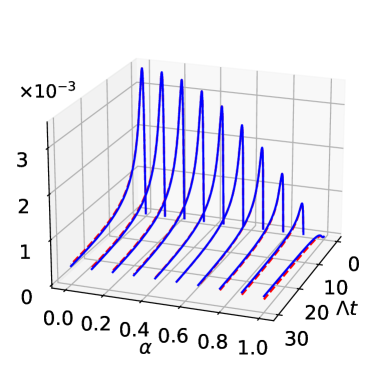
(a)  $\gamma(t)/\Lambda$ in different $\alpha$

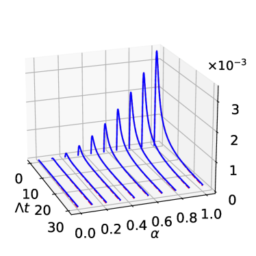
(b)  $\widetilde{\gamma}(t)/\Lambda$ in different $\alpha$

Figure 2: (a) The decay coefficient $\gamma(t)/\Lambda$ and (b) the fluctuation coefficient $\widetilde{\gamma}(t)/\Lambda$ in the time domain for different values of $\alpha=\lvert W_{k}/V_{k}\rvert$, the rate of the pairing strength with the single particle coupling between the system and the environment in the generalized QBM. The exact solution (blue solid line) from Eq. (42) and the estimated solution (red dashed line) based on Eq. (56) agree with each other. Here we set $\gamma_{0}=0.0003\Lambda$, $k_{\textsl{B}}T/\hbar=0.01\Lambda$. They are plotted against time scale $1/\Lambda$ to emphasize the initial jolt. The results show that the initial jolt exists in both the decay coefficient $\gamma(t)$ and the diffusion coefficient $\widetilde{\gamma}(t)$.

With the finding of this accident cancellation of the divergences in the decay coefficient $\gamma(t)$ due to the special choice of $\alpha=1$ in the QBM, the origin of the initial jolt becomes clear. It comes purely from the Ohmic-type spectral densities with the infinite cut-off frequency $\Lambda\rightarrow\infty$. For a fundamental renormalizable theory, one requires that any renormalized quantity must be independent of regularization-scheme, so that the high energy cut-off scale can be taken to the infinite limit in the calculations of energy. However, both the conventional and the generalized QBM are build on phenomenological model Hamiltonians, no such renormalizability is required in priori. Furthermore, the cut-off frequency in the Ohmic-type spectral densities is introduced to count the effective transition processes between the system and the environment. Quantum mechanically, the most active environmental modes $\omega_{k}$ that effectively couple to the system are dominated by these not far away from the thermal frequency $k_{\textsl{B}}T/\hbar$ so that physical transition between the system and the environment can occur (with large probabilities). Physically, the spectral density is a summation of the probabilities over the physical processes between the system and the environment. For the Ohmic-type spectral densities, taking a very large cut-off frequency implies that the environmental modes with higher energy will have the larger probability amplitude for coupling to the system mode. This is obviously very unphysical. The physical reliable cut-off frequency should be estimated by the condition that: the mean frequency of a given spectral density should be the same order of the system characterized frequency, if the system-environment coupling cannot be derived from a more fundamental theory or no experimental data can be used to fix it. Under such a physical requirement, the problem of “initial jolt” will never occur.

V Discussions and Perspectives

In this paper, we provide a detailed analysis on system-environmental couplings which are usually unknown in priori but are the key to the determination of dissipation and fluctuation dynamics in open quantum systems. In particular, we show that the quantum dissipative dynamics described by Feynman-Vernon model and Caldeira-Leggett model based on classical mechanics involve some physically inconsistent processes at quantum level. These inconsistent processes include the transitions from low-energy states to high-energy states by emitting an amount of energy or create particles from nothing, which should be forbidden in quantum mechanics. Within the framework of quantum mechanics, each individual microscopic particle process should be constrained by the conservations of energy-momentum and angular momentum, etc. We further show that one can get rid of these inconsistent processes by including momentum-dependent system-environment couplings. We generalize the QBM to include such momentum-dependent couplings, which are indeed easier to be realized in realistic quantum world. We derive the exact master equation of such generalized QBM for both the initially decoupled and initially correlated system-environment states.

With the generalized QBM and its exact master equation for both the initially decoupled and the initially correlated state, we reproduce the Hu-Paz-Zhang master equation as a special case. We then find that in the Hu-Paz-Zhang equation for the conventional QBM with the position-dependent coupling only, the renormalized Brownian particle Hamiltonian actually contains a renormalization-induced momentum-dependent potential. This momentum-dependent potential is misplaced into the dissipation term in the Hu-Paz-Zhang equation, so that the correct renormalized Brownian particle Hamiltonian was not found before. The environment induced momentum-dependent potential in the Hu-Paz-Zhang equation also indicates that including the momentum-dependent system-environment coupling is a natural consequence of the QBM.

Furthermore, we re-examine the long-standing problem of the initial jolt in the conventional QBM and Hu-Paz-Zhang master equation. The initial jolt is related to the divergence arising from the Ohmic-type spectral density with an infinite cut-off frequency. It has been thought that the initial jolt is a result of using the initial decoupled state which is physically unacceptable, but we find that this is indeed a misunderstanding. The misunderstanding comes from the accident cancellation of the divergences in the decay coefficient in the Hu-Paz-Zhang equation, due to the same coupling strengths for the single particle transition and the pairing processes. With the generalized QBM including the momentum-dependent coupling, we show that the initial jolt exists in both the decay and diffusion coefficients, while the decay coefficient is independent of the initial system-environment state. As a conclusion, the so-called “initial jolt” has nothing do to with the initial decoupled state. It is an artificial effect when one takes an extremely large cut-off frequency in comparison with the thermal energy of the environment, which is unphysical as we explained in the end of the last section.

With the generalized QBM, we have resolved these interesting and important problems for quantum dissipative dynamics, as we discussed in this work. The new exact master equation for the generalized QBM also has the potential applications to photonics quantum computing. With an extension of the generalized QBM to multimodes, one can apply it to the integrated quantum processor made of many squeezers and interferometers with hundred more photonic modes, that currently attracted a great attention in the development of quantum technology. We will leave this problem for further investigation.

Appendix A The generalized nonequilibrium Green functions for open quantum systems with pairing couplings and fluctuation-dissipation theorem

The nonequilibrium Green functions we introduced for open quantum systems Tu2008 ; Jin2010 ; Lei2012 ; Zhang2012 are generalized to open quantum systems involving pairing couplings in this work, and are denoted by $\mathcal{U}(\tau,t_{0})$ and $\mathcal{V}(\tau,t)$ Huang2020 . They are defined as

$$\mathcal{U}(t,t_{0})\mathcal{Z}=\begin{bmatrix}\langle[a(t),a^{\dagger}(t_{0})]\rangle&\langle[a(t),a(t_{0})]\rangle\\ \langle[a^{\dagger}(t),a^{\dagger}(t_{0})]\rangle&\langle[a^{\dagger}(t),a(t_{0})]\rangle\end{bmatrix},$$ (57)

$$\mathcal{V}(\tau,t)=\begin{bmatrix}\langle a^{\dagger}(t)a(\tau)\rangle&\langle a(t)a(\tau)\rangle\\ \langle a^{\dagger}(t)a^{\dagger}(\tau)\rangle&\langle a(t)a^{\dagger}(\tau)\rangle\end{bmatrix}$$

$$\qquad\qquad\qquad\qquad-(\text{initial-dependent part}),$$ (58)

and can be easily determined directly from Heisenberg equation of motion for the generalized QBM Hamiltomnian Eq. (12),

$$\frac{\mathrm{d}}{\mathrm{d}t}\!\begin{bmatrix}a(t)\\ a^{\dagger}(t)\end{bmatrix}=-i\omega_{\textsc{s}}\mathcal{Z}\!\begin{bmatrix}a(t)\\ a^{\dagger}(t)\end{bmatrix}\!-\!i\sum_{k}\mathcal{Z}\!\begin{bmatrix}V_{k}&W_{k}\\ W_{k}^{*}&V_{k}^{*}\\ \end{bmatrix}\!\begin{bmatrix}b_{k}(t)\\ b_{k}^{\dagger}(t)\end{bmatrix},$$ (59a)

$$\frac{\mathrm{d}}{\mathrm{d}t}\!\begin{bmatrix}b_{k}(t)\\ b_{k}^{\dagger}(t)\end{bmatrix}=-i\omega_{k}\mathcal{Z}\!\begin{bmatrix}b_{k}(t)\\ b_{k}^{\dagger}(t)\end{bmatrix}\!-\!i\mathcal{Z}\!\begin{bmatrix}V_{k}^{*}&W_{k}\\ W_{k}^{*}&V_{k}\\ \end{bmatrix}\!\begin{bmatrix}a(t)\\ a^{\dagger}(t)\end{bmatrix}.$$ (59b)

These equations of motion determine all the dissipation and fluctuation dynamics of the Brownian particle.

Formally, solving Eq. (59b), we obtain

$$\begin{bmatrix}b_{k}(t)\\ b_{k}^{\dagger}(t)\end{bmatrix} =\begin{bmatrix}e^{-i\omega_{k}(t-t_{0})}&\!\!0\\ 0&\!\!e^{+i\omega_{k}(t-t_{0})}\end{bmatrix}\!\begin{bmatrix}b_{k}(t_{0})\\ b_{k}^{\dagger}(t_{0})\end{bmatrix}$$

$$\!-\!i\!\!\int_{t_{0}}^{t}\!\!\mathrm{d}\tau\mathcal{Z}\!\begin{bmatrix}V_{k}^{*}(\tau-t)&W_{k}(\tau-t)\\ W_{k}^{*}(\tau-t)&V_{k}(\tau-t)\\ \end{bmatrix}\!\begin{bmatrix}a(\tau)\\ a^{\dagger}(\tau)\end{bmatrix}.$$ (60)

This formal solution allows us to eliminate exactly and completely all the environmental degrees of freedom (equivalent to the trace over all the environment states). Substituting this solution into Eq. (59a), we have

$$\frac{\mathrm{d}}{\mathrm{d}t}\begin{bmatrix}a(t)\\ a^{\dagger}(t)\end{bmatrix}+i\omega_{\textsc{s}}\mathcal{Z}\begin{bmatrix}a(t)\\ a^{\dagger}(t)\end{bmatrix}\!+\!\!\int_{t_{0}}^{t}\!\!\mathrm{d}\tau\mathcal{Z}\mathcal{G}(t,\tau)\!\begin{bmatrix}a(\tau)\\ a^{\dagger}(\tau)\end{bmatrix}$$

$$\qquad\qquad=-i\sum_{k}\mathcal{Z}\!\begin{bmatrix}V_{k}(t-t_{0})&W_{k}(t-t_{0})\\ W_{k}^{*}(t-t_{0})&V_{k}^{*}(t-t_{0})\\ \end{bmatrix}\!\begin{bmatrix}b_{k}(t_{0})\\ b_{k}^{\dagger}(t_{0})\end{bmatrix},$$ (61)

where

$$\mathcal{G}(\tau,\tau^{\prime}) =\!\!\sum_{k}\!\begin{bmatrix}V_{k}(\tau\!-\!t_{0})&\!\!W_{k}(\tau\!-\!t_{0})\\ W_{k}^{*}(\tau\!-\!t_{0})&\!\!V_{k}^{*}(\tau\!-\!t_{0})\end{bmatrix}$$

$$\qquad\times\!\!\begin{bmatrix}1&0\\ 0&-1\end{bmatrix}\!\!\begin{bmatrix}V_{k}^{*}(\tau^{\prime}\!-\!t_{0})&\!\!W_{k}(\tau^{\prime}\!-\!t_{0})\\ W_{k}^{*}(\tau^{\prime}\!-\!t_{0})&\!\!V_{k}(\tau^{\prime}\!-\!t_{0})\end{bmatrix}$$ (62)

is Eq. (30a). One can clearly see that Eq. (61) is the generalized quantum Langevin equation, in which the third term in the left hand side is the dissipation (decay) term due to the system-environment coupling, and the term in the right hand side is the fundamental noise force generated by the environment through the system-environment coupling. It is obvious that the average of the noise force is zero if the environment is initially in a thermal state.

Because Eq.(61) is a linear differential equation, its general solution has the form

$$\begin{bmatrix}a(t)\\ a^{\dagger}(t)\end{bmatrix}=\mathcal{U}(t,t_{0})\begin{bmatrix}a(t_{0})\\ a^{\dagger}(t_{0})\end{bmatrix}+\begin{bmatrix}F(t)\\ F^{\dagger}(t)\end{bmatrix}.$$ (63)

Substituting this general solution into Eq. (61), one can find that the retarded Green function $\mathcal{U}(t,t_{0})$ describes the dissipation dynamics of the Brownian particle and obeys the Dyson equation of motion,

$$\frac{\mathrm{d}}{\mathrm{d}\tau}\mathcal{U}(\tau,t_{0})\!+\!i\omega_{\textsc{s}}\mathcal{Z}\mathcal{U}(\tau,t_{0})\!+\!\!\int_{t_{0}}^{\tau}\!\!\!\mathrm{d}\tau^{\prime}\mathcal{Z}\mathcal{G}(\tau,\tau^{\prime})\mathcal{U}(\tau^{\prime},t_{0})=0,$$ (64)

which is just Eq. (35a). The integral kernel in the above equation characterize the non-Markovian dissipation processes. It is easy to show that the definition of the retarded Green function $\mathcal{U}(t,t_{0})$ in Eq. (63) is the same as the definition of Eq. (57),

$$\begin{bmatrix}\langle[a(t),a^{\dagger}(t_{0})]\rangle&\langle[a(t),a(t_{0})]\rangle\\ \langle[a^{\dagger}(t),a^{\dagger}(t_{0})]\rangle&\langle[a^{\dagger}(t),a(t_{0})]\rangle\end{bmatrix}$$

$$\qquad=\mathcal{U}(t,t_{0})\begin{bmatrix}\langle[a(t_{0}),a^{\dagger}(t_{0})]\rangle&\langle[a(t_{0}),a(t_{0})]\rangle\\ \langle[a^{\dagger}(t_{0}),a^{\dagger}(t_{0})]\rangle&\langle[a^{\dagger}(t_{0}),a(t_{0})]\rangle\end{bmatrix}$$

$$\qquad=\mathcal{U}(t,t_{0})\mathcal{Z}.$$ (65)

The last term in Eq. (63) describes the environment-induced fluctuation (noise) dynamics that obeys the following equation of motion,

$$\frac{\mathrm{d}}{\mathrm{d}t}\begin{bmatrix}F(t)\\ F^{\dagger}(t)\end{bmatrix}+i\omega_{\textsc{s}}\mathcal{Z}\begin{bmatrix}F(t)\\ F^{\dagger}(t)\end{bmatrix}\!+\!\!\int_{t_{0}}^{t}\!\!\mathrm{d}\tau\mathcal{Z}\mathcal{G}(t,\tau)\!\begin{bmatrix}F(\tau)\\ F^{\dagger}(\tau)\end{bmatrix}$$

$$\qquad\qquad=-i\sum_{k}\mathcal{Z}\begin{bmatrix}V_{k}(t-t_{0})&W_{k}(t-t_{0})\\ W_{k}^{*}(t-t_{0})&V_{k}^{*}(t-t_{0})\\ \end{bmatrix}\!\begin{bmatrix}b_{k}(t_{0})\\ b_{k}^{\dagger}(t_{0})\end{bmatrix},$$ (66)

subjected to the initial condition $\Big{[}\begin{smallmatrix}F(t_{0})\\ F^{\dagger}(t_{0})\end{smallmatrix}\Big{]}=0$. From this initial condition, the general solution of the equation for the noise dynamics is given explicitly,

$$\begin{bmatrix}F(t)\\ F^{\dagger}(t)\end{bmatrix}$$

$$=-i\!\sum_{k}\!\!\int_{t_{0}}^{t}\!\!\mathrm{d}\tau\mathcal{U}(t,\tau)\mathcal{Z}\!\begin{bmatrix}V_{k}(t-t_{0})&\!W_{k}(t-t_{0})\\ W_{k}^{*}(t-t_{0})&\!V_{k}^{*}(t-t_{0})\\ \end{bmatrix}\!\!\begin{bmatrix}b_{k}(t_{0})\\ b_{k}^{\dagger}(t_{0})\end{bmatrix}.$$ (67)

The nonequilibrium correlation functions are defined by

$$\begin{bmatrix}\langle a^{\dagger}(t)a(\tau)\rangle&\langle a(t)a(\tau)\rangle\\ \langle a^{\dagger}(t)a^{\dagger}(\tau)\rangle&\langle a(t)a^{\dagger}(\tau)\rangle\end{bmatrix}$$

$$\qquad=\mathcal{U}(\tau,t_{0})\begin{bmatrix}\langle a^{\dagger}(t_{0})a(t_{0})\rangle&\langle a(t_{0})a(t_{0})\rangle\\ \langle a^{\dagger}(t_{0})a^{\dagger}(t_{0})\rangle&\langle a(t_{0})a^{\dagger}(t_{0})\rangle\end{bmatrix}\mathcal{U}^{\dagger}(t,t_{0})$$

$$\qquad\qquad\qquad+\begin{bmatrix}\langle F^{\dagger}(t)F(\tau)\rangle&\langle F(t)F(\tau)\rangle\\ \langle F^{\dagger}(t)F^{\dagger}(\tau)\rangle&\langle F(t)F^{\dagger}(\tau)\rangle\end{bmatrix}.$$ (68)

The last term is the noise-induced correlation Green function $\mathcal{V}(\tau,t)$, which has the solution

$$\mathcal{V}(\tau,t) =\begin{bmatrix}\langle F^{\dagger}(t)F(\tau)\rangle&\langle F(t)F(\tau)\rangle\\ \langle F^{\dagger}(t)F^{\dagger}(\tau)\rangle&\langle F(t)F^{\dagger}(\tau)\rangle\end{bmatrix}$$

$$=\!\!\int_{t_{0}}^{\tau}\!\!\mathrm{d}\tau^{\prime}\!\!\int_{t_{0}}^{t}\!\!\mathrm{d}t^{\prime}\mathcal{U}(\tau,\tau^{\prime})\mathcal{Z}\widetilde{\mathcal{G}}(\tau^{\prime},t^{\prime})\mathcal{Z}\mathcal{U}^{\dagger}(t,t^{\prime}).$$ (69)

This gives the same solution Eq. (37) obtained in our exact master equation derivation. The initial-state-dependent system-environment correlation function $\widetilde{\mathcal{G}}(t,t^{\prime})$ is given by

$$\widetilde{\mathcal{G}}(\tau^{\prime},t^{\prime}) =\sum_{k}\begin{bmatrix}V_{k}(\tau^{\prime}-t_{0})&W_{k}(\tau^{\prime}-t_{0})\\ W_{k}^{*}(\tau^{\prime}-t_{0})&V_{k}^{*}(\tau^{\prime}-t_{0})\\ \end{bmatrix}$$

$$\qquad\quad\times\begin{bmatrix}\langle b_{k}^{\dagger}(t)b_{k}(\tau)\rangle&\langle b_{k}(t)b_{k}(\tau)\rangle\\ \langle b_{k}^{\dagger}(t)b_{k}^{\dagger}(\tau)\rangle&\langle b_{k}(t)b_{k}^{\dagger}(\tau)\rangle\end{bmatrix}$$

$$\qquad\quad\times\begin{bmatrix}V_{k}^{*}(t^{\prime}-t_{0})&W_{k}(t^{\prime}-t_{0})\\ W_{k}^{*}(t^{\prime}-t_{0})&V_{k}(t^{\prime}-t_{0})\\ \end{bmatrix},$$ (70)

which is Eq. (30b). The solution Eq. (69) is also the generalization of the Keldysh’s correlation function in the nonequilibrium technique Keldysh1965 . It is indeed the generalized nonequilibrium fluctuation-dissipation theorem, as a consequence of the unitarity principle of quantum mechanics for the whole system (the system plus the environment) Zhang2012 . The usual equilibrium fluctuation-dissipation theorem can be easily obtained from this solution as a steady-state limit.

References

• (1) H. Grabert, P. Schramm, and G.-L. Ingold, Quantum Brownian motion: The functional integral approach, Phys. Rep. 168, 115 (1988).
• (2) U. Weiss, Quantum Dissipative Systems, 4th Edition (World Scientific, Singapore, 2012).
• (3) R. P. Feynman and F. L. Vernon, The theory of a general quantum system interacting with a linear dissipative system, Ann. Phys. 24, 118 (1963).
• (4) A. O. Caldeira and A. J. Leggett, Path integral approach to quantum Brownian motion, Physica 121A, 587 (1983).
• (5) A. O. Caldeira and A. J. Leggett, Quantum Tunnelling in a Dissipative System, Ann. Phys. 149, 374 (1983).
• (6) F. Haake and R. Reibold, Strong damping and low-temperature anomalies for the harmonic oscillator, Phys. Rev. A 32, 2462 (1985).
• (7) B. L. Hu, J. P. Paz, and Y. H. Zhang, Quantum Brownian motion in a general environment: Exact master equation with nonlocal dissipation and colored noise, Phys. Rev. D 45, 2843 (1992).
• (8) R. Karrlein and H. Grabert, Exact time evolution and master equations for the damped harmonic oscillator, Phys. Rev. E 55, 153 (1997).
• (9) H. Zheng, S. Y. Zhu, and M. S. Zubairy, Quantum Zeno and Anti-Zeno Effects: Without the Rotating-Wave Approximation, Phys. Rev. Lett. 101, 200404 (2008).
• (10) T. Niemczyk, F. Deppe, H. Huebl, E. P. Menzel, F. Hocke, M. J. Schwarz, J. J. Garcia-Ripoll, D. Zueco, T. Hummer, E. Solano, A. Marx, and R. Gross, Circuit quantum electrodynamics in the ultrastrong-coupling regime Nat. Phys. 6 772 (2010).
• (11) Y. Li, J. Evers, W. Feng, and S. Y. Zhu, Spectrum of collective spontaneous emission beyond the rotating-wave approximation, Phys. Rev. A 87, 053837 (2013).
• (12) L. Garziano, V. Macrì, R. Stassi, O. D. Stefano, F. Nori, and S. Savasta, One photon can simultaneously excite two or more atoms, Phys. Rev. Lett. 117, 043601 (2016).
• (13) D. Z. Xu and J. S. Cao, Non-canonical distribution and non-equilibrium transport beyond weak system-bath coupling regime: A polaron transformation approach, Front. Phys. 11, 110308 (2016).
• (14) X. Wang, A. Miranowicz, H. R. Li, and F. Nori, Observing pure effects of counter-rotating terms without ultrastrong coupling: A single photon can simultaneously excite two qubits, Phys. Rev. A 96, 063820 (2017).
• (15) F. Yoshihara, T. Fuse, S. Ashhab, K. Kakuyanagi, S. Saito, and K. Semba, Superconducting qubit-oscillator circuit beyond the ultrastrong-coupling regime, Nat. Phys. 13, 44 (2017).
• (16) C. Cohen-Tannoudji, J. Dupont-Roc, and G. Grynberg, Atom-Photon Interactions: Basic Process and Applications, (Wiley-Vch, 1998).
• (17) R. P. Feynman and A. R. Hibbs, Quantum Mechanics and Path Integrals, (New York, McGraw-Hill, 1965).
• (18) M. E. Peskin and D. V. Schroeder, An Introduction to Quantum Field Theory, (Addison Wesley, New York, 1995).
• (19) S. Aaronson and A. Arkhipov, The Computational Complexity of Linear Optics, in Proceedings of the 43rd Annual ACM Symposium on Theory of Computing, 333 (ACM Press, 2011).
• (20) A. Crespi, R. Osellame, R. Ramponi, D. J. Brod, E. F. Galvão, N. Spagnolo, C. Vitelli, E. Maiorino, P. Mataloni, and F. Sciarrino, Integrated multimode interferometers with arbitrary designs for photonic boson sampling, Nat. Photonics, 7, 545 (2013).
• (21) H. S. Zhong, H. Wang, Y. H. Deng, M. C. Chen, L. C. Peng, Y. H. Luo, J. Qin, D. Wu, X. Ding, Y. Hu, P. Hu, X. Y. Yang, W. J. Zhang, H. Li, Y. X. Li, X. Jiang, L. Gan, G. W. Yang, L. X. You, Z. Wang, L. Li, N. L. Liu, C. Y. Lu, and J. W. Pan, Quantum computational advantage using photons, Science 370, 1460 (2020).
• (22) H. S. Zhong, Y. H. Deng, J. Qin, H. Wang, M. C. Chen, L. C. Peng, Y. H. Luo, D. Wu, S. Q. Gong, H. Su, Y. Hu, P. Hu, X. Y. Yang, W. J. Zhang, H. Li, Y. X. Li, X. Jiang, L. Gan, G. W. Yang, L. X. You, Z. Wang, L. Li, N. L. Liu, J. J. Renema, C. Y. Lu, and J. W. Pan, Phase-Programmable Gaussian Boson Sampling Using Stimulated Squeezed Light, Phys. Rev. Lett. 127, 180502 (2021).
• (23) A. Politi, J. C. F. Matthews, M. G. Thompson, and J. L. O’Brien, Integrated Quantum Photonics, IEEE J. Sel. Top. Quantum Electron. 15, 1673 (2009).
• (24) S. Paesani, Y. Ding, R. Santagati, L. Chakhmakhchyan, C. Vigliar, K. Rottwitt, L. K. Oxenløwe, J. W. Wang, M. G. Thompson, and A. Laing, Generation and sampling of quantum states of light in a silicon chip, Nat. Phys. 15, 925 (2019).
• (25) A. W. Elshaari, W. Pernice, K. Srinivasan, O. Benson, and V. Zwiller, Hybrid integrated quantum photonic circuits, Nat. Photonics 14, 285 (2020).
• (26) J. M. Arrazola, V. Bergholm, K. Brádler, T. R. Bromley1, M. J. Collins, I. Dhand, A. Fumagalli, T. Gerrits, A. Goussev, L. G. Helt, J. Hundal, T. Isacsson, R. B. Israel, J. Izaac, S. Jahangiri, R. Janik, N. Killoran, S. P. Kumar, J. Lavoie, A. E. Lita, D. H. Mahler, M. Menotti, B. Morrison, S. W. Nam, L. Neuhaus, H. Y. Qi, N. Quesada, A. Repingon, K. K. Sabapathy, M. Schuld, D. Su, J. Swinarton, A. Száva, K. Tan, P. Tan, V. D. Vaidya, Z. Vernon, Z. Zabaneh, and Y. Zhang, Quantum circuits with many photons on a programmable nanophotonic chip, Nature 591, 54 (2021).
• (27) D. N. Liu, J. Y. Zheng, L. J. Yu, X. Feng, F. Liu, K. Y. Cui, Y. D. Huang, and W. Zhang, Generation and dynamic manipulation of frequency degenerate polarization entangled Bell states by a silicon quantum photonic circuit, Chip 1, 1 (2022).
• (28) L. Fu and C. L. Kane, Superconducting proximity effect and Majorana fermions at the surface of a topological insulator, Phys. Rev. Lett. 100, 096407 (2008).
• (29) J. D. Sau, R. M. Lutchyn, S. Tewari, and S. D. Sarma, Generic new platform for topological quantum computation using semiconductor heterostructures, Phys. Rev. Lett. 104, 040502 (2010).
• (30) Y. Oreg, G. Refael, and F. von Oppen, Helical liquids and Majorana bound states in quantum wires, Phys. Rev. Lett. 105, 177002 (2010).
• (31) R. M. Lutchyn, E. P. A. M. Bakkers, L. P. Kouwenhoven, P. Krogstrup, C. M. Marcus, and Y. Oreg, Majorana zero modes in superconductor-semiconductor heterostructures, Nature Review Materials, 3, 52 (2018).
• (32) Y. W. Huang, P. Y. Yang, and W. M. Zhang, Quantum theory of dissipative topological systems, Phys. Rev. B 102, 165116 (2020).
• (33) H. L. Lai, P. Y. Yang, Y. W. Huang, and W. M. Zhang, Exact master equation and non-Markovian decoherence dynamics of Majorana zero modes under gate-induced charge fluctuations, Phys. Rev. B 97, 054508 (2018).
• (34) H. L. Lai and W. M. Zhang, Decoherence dynamics of Majorana qubits under braiding operations, Phys. Rev. B 101, 195428 (2020).
• (35) C. Z. Yao and W. M. Zhang, Probing topological states through the exact non-Markovian decoherence dynamics of a spin coupled to a spin bath in real-time domain, Phys. Rev. B 102, 035133 (2020).
• (36) F. L. Xiong, H. L. Lai, and W. M. Zhang, Manipulating Majorana qubit states without braiding, Phys. Rev. B 104, 205417 (2021).
• (37) B. Simon, The classical limit of quantum partition functions, Commun. Math. Phys. 71, 247 (1980).
• (38) J. von Neumann, Mathematische Grundlagen der Quantenmechanik, (Springer, Berlin, 1932), also Mathematical foundations of quantum mechanics, translated by R. T. Beyer, (Princeton university press, 1955).
• (39) W. M. Zhang, D. H. Feng, and R. Gilmore, Coherent States: Theory and some applications, Rev. Mod. Phys. 62, 867 (1990).
• (40) J. Jin, M. W. Y. Tu, W. M. Zhang, and Y. J. Yan, Non-equilibrium quantum theory for nanodevices based on the Feynman–Vernon influence functional, New. J. Phys. 12, 083013 (2010).
• (41) L. D. Faddeev and A. A. Slavnov, Gauge Fields: Introduction to Quantum Theory, (Benjamin-Cummings, Reading, MA, 1980).
• (42) C. U Lei and W. M. Zhang, A quantum photonic dissipative transport theory, Ann. Phys. 327, 1408 (2012).
• (43) M. W. Y. Tu and W. M. Zhang, Non-Markovian decoherence theory for a double-dot charge qubit, Phys. Rev. B 78, 235311 (2008).
• (44) W. M. Zhang, P. Y. Lo, H. N. Xiong, M. W. Y. Tu, and F. Nori, General non-Markovian dynamics of open quantum systems, Phys. Rev. Lett. 109, 170402 (2012).
• (45) L. V. Keldysh, Diagram technique for nonequilibrium processes, Sov. Phys. JETP 20, 1018 (1965).
• (46) It may be worth pointing out that the Lindblad superoperators proposed in terms of memory-less dynamical maps actually do not relate to the fundamental degrees of freedom in open quantum systems. The mathematical construction of dynamical generators in GKSL master equation Lindblad1976 ; GKS1976 is based on the dimension of the finite Hilbert space of the system, which are very different from these fundamental generators for generating the Hilbert space of the system. The later forms the Lie algebra, whose dimension is much smaller than its unitary representation space except for the faithful representation. In the literature, people often misused the corresponding concept.
• (47) G. Lindblad, On the generators of quantum dynamical semigroups, Commun. Math. Phys. 48, 119 (1976).
• (48) V. Gorini, A. Kossakowski, and E. C. G. Sudarshan, Completely positive dynamical semigroups of N-level systems, J. Math. Phys. 17, 821 (1976).
• (49) H. N. Xiong, W. M. Zhang, X. G. Wang, and M. H. Wu, Exact non-Markovian cavity dynamics strongly coupled to a reservoir, Phys. Rev. A 82, 012105 (2010).
• (50) M. H. Wu, C. U Lei, W. M. Zhang, and H. N. Xiong, Non-Markovian dynamics of a microcavity coupled to a waveguide in photonic crystals, Opt. Express 18, 18407 (2010).
• (51) C. U Lei and W. M. Zhang, Decoherence suppression of open quantum systems through a strong coupling to non-Markovian reservoirs, Phys. Rev. A 84, 052116 (2011).
• (52) H. T. Tang and W. M. Zhang, Non-Markovian dynamics of open quantum systems with initial system-bath correlations: A nanocavity coupled to a coupled resonator optical waveguide, Phys. Rev. A 83, 032102 (2011).
• (53) H. N. Xiong, P. Y. Lo, W. M. Zhang, D. H. Feng, and F. Nori, Non-Markovian Complexity in the Quantum-to-Classical Transition, Sci. Rep. 5, 13353 (2015).
• (54) W. G. Unruh and W. H. Zurek, Reduction of a wave packet in quantum Brownian motion, Phys. Rev. D 40, 1071 (1989).
• (55) G. W. Ford, J. T. Lewis, and R. F. O’Connell, Quantum measurement and decoherence, Phys. Rev. A 64, 032101 (2001).