Hybrid Cloud-Edge Collaborative Data Anomaly Detection in Industrial Sensor Networks

Abstract

Industrial control systems (ICSs) are facing increasing cyber-physical attacks that can cause catastrophes in the physical system. Efficient anomaly detection models in the industrial sensor networks are essential for enhancing ICS reliability and security, due to the sensor data is related to the operational state of the ICS. Considering the limited availability of computing resources, this paper proposes a hybrid anomaly detection approach in cloud-edge collaboration industrial sensor networks. The hybrid approach consists of sensor data detection models deployed at the edges and a sensor data analysis model deployed in the cloud. The sensor data detection model based on Gaussian and Bayesian algorithms can detect the anomalous sensor data in real-time and upload them to the cloud for further analysis, filtering the normal sensor data and reducing traffic load. The sensor data analysis model based on Graph convolutional network, Residual algorithm and Long short-term memory network (GCRL) can effectively extract the spatial and temporal features and then identify the attack precisely. The proposed hybrid anomaly detection approach is evaluated using a benchmark dataset and baseline anomaly detection models. The experimental results show that the proposed approach can achieve an overall 11.19% increase in Recall and an impressive 14.29% improvement in F1-score, compared with the existing models.

I Introduction

Currently, the industrial control systems (ICSs) exhibit heterogeneous, federated, large-scale and intelligent characteristics due to the increasing number of the Internet of Things (IoT) devices and the corresponding sensors deployed in industrial sensor networks [1]. However, the massive penetration of advanced IoT devices leads the ICS to be cyber-physical systems that may suffer from cyber-physical threats and attacks. These IoT devices are prone to the backdoors that can be used by attackers to launch severe attacks. It is indicated in [2] that the growth rate of IoT vulnerabilities was 14.7% higher than that of network vulnerabilities. The behaviors of intruders will affect the operational state of the ICS, and the sensor data is related to the state of the ICS [3]. Therefore, anomalous sensor data detection can be considered a key countermeasure against cyber-physical attacks [4].

The control center can analyze the data collected by a lot of sensors and then deliver various commands to the connected system, which will improve the operational benefits of reliability, safety and control. However, if the massive sensors are analyzed by centralized management, it is difficult to meet the requirement of real-time operation in the ICSs. To control and analyze such massive IoT devices and connected sensors, a cloud-edge computing environment is a key technology [5]. Some anomaly detection models adopt distributed detection method based on a statistical algorithm due to the limited computational resources of the edges, with a low detection precision and recall. Therefore, most of the existing anomaly detection models adopt centralized detection for obtaining high detection precision and recall, which will collect each sensor data and then process and analyze it, resulting in heavy traffic load. The increase in traffic load may lead to many serious problems, e.g., loss of control commands and packet corruption in ICS. In this paper, the hybrid anomaly detection approach through cloud-edge collaboration in industrial sensor networks is proposed for reducing the heavy traffic load and improving detection precision and recall, consisting of a set of sensor data anomaly detection models at the edges and a sensor data analysis model in the cloud. An anomaly detection model based on statistical methods deployed at the edges can detect and only upload anomalous sensor data so that it can filter massive normal sensor data and make traffic load smaller, considering the limited computing resources. However, these detected anomalous sensor data may contain amounts of normal data due to the simple computing structure of the statistical algorithms, leading to a low detection precision and recall. Therefore, we use an anomaly analysis model based on deep learning algorithms deployed in the cloud, which can further analyze the uploaded sensor data and improve detection precision and recall.

The sensor data detection model based on Gaussian and Bayesian algorithms [6] deployed at the edge areas can detect the anomalous sensor data by calculating the probability of anomaly and then make them available to the cloud for further analysis, filtering massive normal sensor data and making traffic load smaller.

The industrial sensor networks are graph-structure data, containing spatial and temporal features [7], in which the sensors are nodes, and the link between two sensors is the edge. Moreover, the features of the nodes are the values of sensors. Therefore, we need an analysis model that can not only consider the spatial features but also can extract the temporal features. The graph convolutional network (GCN) is considered a component in our analysis model, which is widely used in processing graph-structured data for extracting spatial features [8]. The input of the GCN consists of a feature matrix, i.e., sensor data and an adjacency matrix that represents the complex correlation between different sensors in the industrial sensor network. To visualize the adjacency matrix, the sensor data correlation graph, in which the nodes are the sensors and the edge between any two sensors represents the existing correlation, is used in this work. The topology of the sensor network cannot represent the correlation between any two sensors [9]. Therefore, this work adopts the Spearman correlation analysis algorithm [10] to construct the adjacency matrix as one of the inputs of GCN. The measurements from sensors are time-series data that contains many temporal features. However, it is considered the efficient extraction of the temporal features can be hardly implemented only using the GCN because its calculation is conducted in the spatial domain. Thus, the long short-term memory (LSTM) [11] is incorporated into the proposed model for extracting temporal information. Furthermore, the Residual method [12] is also considered to address the problem of gradient disappearance. The sensor data analysis model based on graph convolutional network, residual algorithm and long short-term memory network (i.e. GCRL) in the cloud is proposed to further analyze the sensor data uploaded by the detection model at the edge and then accurately identify the attacks. The main contributions made in this work are as follows:

(1) A hybrid cloud-edge collaborative anomaly detection framework with high detection precision and recall for the industrial sensor network is developed that combines statistical and deep learning models, which can also make traffic load smaller.

(2) The Spearman correlation analysis algorithm is adopted to generate the sensor data correlation graph and a novel deep learning analysis model, i.e. GCRL is proposed, which can learn the relationship of different sensors and extract the temporal features.

(3) The proposed solution is assessed through experiments based on a benchmark industrial sensor dataset. The results demonstrate that the proposed approach can achieve an overall 11.19% increase in Recall and an impressive 14.29% improvement in F1-score, compared with the existing models.

The rest of the paper is organized as follows: Section II discusses the existing anomaly detection solutions in industrial sensor networks. The proposed hybrid cloud-edge collaborative anomaly detection approach for industrial sensor networks is presented in Section III. The experimental results of the proposed approach are compared with existing baseline approaches in Section IV. The conclusions and future research directions are given in Section V.

II Related Work

In the literature, the anomaly detection models based on statistical algorithms are widely used in an industrial sensor network. The principal component analysis (PCA) algorithm is used for anomaly detection, assuming the anomalies can be treated as outliers [13]. The author proposed a mixture of probabilistic PCA models for fault detection, which can separate the input space into some local regions and deployed the linear sensor anomaly diagnosis model in each region [14]. A novel sparse PCA model can complete the task of localizing anomalies by analyzing a sparse low-dimensional space of anomalous data [15]. In [16], the author proposed a distributed anomaly detection technique based on the seasonal autoregressive integrated moving average (SARIMA), considering the limited computing resources. In [17], a data-driven detection approach was developed based on hidden Markov models in the industrial sensor network. However, the anomaly detection models based on statistical algorithms have a low detection precision and recall.

Machine learning-based methods have also been widely exploited in anomaly detection systems. In [18], the normal sensor data was adopted to train the generative adversarial network (GAN), and the discriminator based on the LSTM-Recurrent neural network was used to compute anomaly scores. However, the detection precision of this model is low in a benchmark dataset. In [19], the author proposed a GAN-based anomaly detection model using the value of a heart rate sensor and an accelerometer. In [20], the author developed an anomaly detection framework based on federated learning, combing CNN with LSTM. Moreover, the model in [21] consisted of CNN and LSTM. In [22], the author proposed an explainable anomaly detection method based on Bi-directional LSTM (BiLSTM). In [23], the LSTM was used in a Variational AutoEncoder (VAE), and the model can measure anomaly score by calculating reconstruction error. The author developed an anomaly detection model based on artificial neural networks using a real industrial dataset for testing [24]. The authors [25] reduced the dimensionality of the sensor data and identified the anomalous data based on autoencoders. In [26], the author proposed an autoencoder to identify the outlier. However, these machine learning-based models only focus on the temporal features without considering the spatial features of sensor data.

In recent years, graph neural network (GNN) models have been exploited for spatial features extraction in industrial sensor networks. The graph deviation network (GDN) [27] was used to predict the future data by graph attention-based forecasting and the absolute error was computed for evaluating the graph deviation score. In [28], a framework for sensor data anomaly detection was proposed, consisting of automatically learning a graph structure, graph convolutional and transformer. However, these two models cannot efficiently extract the spatial and temporal features, with a low recall and F1-score in a benchmark. Furthermore, anomaly detection models based on statistical and deep learning algorithms are popular. The author proposed an LSTM-Gauss-NBayes approach [29], which combined the LSTM with the Gaussian Bayes model for anomaly detection in the sensor network. However, this approach has a high false-positive rate dealing with non-Gaussian distribution data. The author proposed a low-complexity model to detect anomalous sensor data in an industrial sensor network [30]. This model utilized the sensor data to compute the temporal correlation using the autocorrelation function (ACF) and the genetic algorithm (GA) was used to solve multiobjective optimization. In [31], the authors developed a deep autoencoding gaussian model to identify anomalous data, consisting of a gaussian mixture model and deep autoencoders. It should be noted that the machine learning-based model can be computationally complex for the edges of the industrial sensor network with limited computational capability, and hence can be hardly deployed in the field sensors in practice. Therefore, most of the existing anomaly detection models adopt centralized detection deployed in the cloud, leading to the heavy traffic load in the ICSs.

III FRAMEWORK OF PROPOSED HYBRID CLOUD-EDGE COLLABORATIVE ANOMALY DETECTION APPROACH

III-A Data Preprocessing

In this work, the data preprocessing is carried out based on the aggregation algorithm and the Box-Cox transformation algorithm [30]. In reality, the collected sensor measurement data may be incorrect due to the network or the sensor faults. In addition, the data sampling rate is generally high, e.g., at the time-scales of second or millisecond, the aggregation algorithm can be adopted for data aggregation to examine the data behavior over a time period. The aggregated sensor data may not follow the Gaussian distribution, so the Box-Cox transformation is used to transform the non-Gaussian distribution data into a Gaussian distribution. The details of the data preprocessing are given in equations (1)-(2).

$$\centering X_{r,i,t}=x_{r,i,t}+x_{r,i,t+a}+\cdots+x_{r,i,t+Ba}\@add@centering$$ (1)

$$\centering X_{r,i,t}^{\prime}=\left\{\begin{array}[]{l}\frac{X_{r,i,t}-1}{\lambda_{r,i}}\text{ if }\lambda_{r,i}\neq 0\\ \log\left[X_{r,i,t}\right]\text{ if }\lambda_{r,i}=0\end{array}\right.\@add@centering$$ (2)

where $x_{r,i,t}$ represents the collected original data of sensor $i$ in the $r$-th edge at time $t$; $a$ is the sampling period and $B$ is the scale of aggregation; $X_{r,i,t}$ is the aggregated data of sensor $i$ in the $r$-th edge at time $t$. $\lambda_{r,i}$ is used to maximize the log-likelihood function of sensor $i$ in the $r$-th edge. $X_{r,i,t}^{{}^{\prime}}$ is the preprocessed data of sensor $i$ in the $r$-th edge at time $t$.

III-B Sensor data detection model based on Gaussian and Bayesian algorithms at the edge

Each edge consists of some sensors and a sensor data detection model based on Gaussian and Bayesian algorithms [6]. The dataset is split into two sets: a training set and a testing set, in which the label value 0 represents abnormal and 1 represents normal. The probability density function (PDF) of normal and abnormal data is obtained for individual sensors based on equation (3).

$$\centering\left\{\begin{array}[]{l}f_{r,i,no}=\frac{1}{\sqrt{2\pi}\delta_{r,i,no}}\exp\left(\frac{\left(X_{r,i,t}^{\prime}-\mu_{r,i,no}\right)^{2}}{2\delta_{r,i,no}^{2}}\right)\\ f_{r,i,ab}=\frac{1}{\sqrt{2\pi}\delta_{r,i,ab}}\exp\left(\frac{\left(X_{r,i,t}^{\prime}-\mu_{r,i,ab}\right)^{2}}{2\delta_{r,i,ab}^{2}}\right)\end{array}\right.\@add@centering$$ (3)

where $f_{r,i,no}$ and $f_{r,i,ab}$ represents the normal and abnormal PDF of sensor $i$ in the $r$-th edge, respectively; $\mu_{r,i,no}$ and $\delta_{r,i,no}$ are the means and variance of the $i$-th sensor in the $r$-th edge when its label is 1. Otherwise, it is $\mu_{r,i,ab}$ and $\delta_{r,i,ab}$, respectively.

The parameters of normal and abnormal PDF can be obtained from the maximum likelihood estimate in the preprocessed training sensor data set that include normal and abnormal data. The parameters of PDF are shown as in equation (4):

$$\centering\left\{\begin{array}[]{l}\mu_{r,i,no}=\overline{X_{r,i,no}^{\prime}}\\ \mu_{r,i,ab}=\overline{X_{r,i,ab}^{\prime}}\\ \delta_{r,i,no}=\frac{1}{n_{1}}\sum_{j=1}^{n_{1}}\left(X_{r,i,j,no}^{\prime}-\overline{X_{r,i,no}^{\prime}}\right)^{2}\\ \delta_{r,i,ab}=\frac{1}{n_{0}}\sum_{j=1}^{n_{0}}\left(X_{r,i,j,ab}^{\prime}-\overline{X_{r,i,ab}^{\prime}}\right)^{2}\end{array}\right.\@add@centering$$ (4)

where $\overline{X_{r,i,no}^{\prime}}$ and $\overline{X_{r,i,ab}^{\prime}}$ represents the means in normal and abnormal training sets of $i$-th sensor data in the $r$-th edge, respectively. $X_{r,i,j,no}^{\prime}$ and $X_{r,i,j,ab}^{\prime}$ represents the preprocessed $j$-th abnormal and normal data of sensor $i$ in the $r$-th edge, respectively. $n_{0}$ and $n_{1}$ are the number of preprocessed abnormal and normal training data of sensor $i$ in the $r$-th edge, respectively.

Thus, the normal and abnormal probability of the sensor data can be calculated based on equation (5).

$$\centering\!\!\left\{\begin{array}[]{l}\!\!\!\!p\left(y=1\mid X_{r,i,j}^{\prime}\right)\!\!=\!\frac{p\left(X_{r,i,t}^{\prime}\mid y=1\right)p(y=1)}{p\left(X_{r,i,t}^{\prime}\mid y=1\right)p(y=1)+p\left(X_{r,i,t}^{\prime}\mid y=0\right)p(y=0)}\\ \!\!\!\!p\left(y=0\mid X_{r,i,j}^{\prime}\right)\!\!=\!\frac{p\left(X_{r,i,t}^{\prime}\mid y=0\right)p(y=0)}{p\left(X_{r,i,t}^{\prime}\mid y=1\right)p(y=1)+p\left(X_{r,i,t}^{\prime}\mid y=0\right)p(y=0)}\end{array}\right.\@add@centering$$ (5)

As the $p\left(X_{r,i,j}^{\prime}\mid y=1\right)$$p(y=1)$$+$$p\left(X_{r,i,j}^{\prime}\mid y=0\right)$$p(y=0)$, i.e., the denominator is the same when $p\left(y=1\mid X_{r,i,j}^{\prime}\right)$ and $p\left(y=0\mid X_{r,i,j}^{\prime}\right)$ are compared. Thus, equation (5) can be further simplified as equation (6).

$$\centering\left\{\begin{array}[]{l}p\left(y=1\mid X_{r,i,t}^{\prime}\right)=f_{r,i,no}\left(X_{r,i,t}^{\prime}\right)p(y=1)\\ p\left(y=0\mid X_{r,i,t}^{\prime}\right)=f_{r,i,ab}\left(X_{r,i,t}^{\prime}\right)p(y=0)\end{array}\right.\@add@centering$$ (6)

where $p(y=1)$ and $p(y=0)$ are constants, which represent the proportion of normal and abnormal samples in the training set, respectively.

The algorithm of the sensor data detection model is given in Algorithm 1: where $k$ is the number of edge areas in the sensor network; $m_{r}$ is the number of sensors in the $r$-th edge. And $F_{t}$ represents $\left[x_{-}ab_{r,i,t},x_{-}ab_{r,i,t+a},\cdots,x_{-}ab_{r,i,t+Ba}\right]$.

Not all sensor data can be transformed into Gaussian distribution using the Box-Cox algorithm. Therefore, the $p\left(y=1\mid X_{r,i,t}^{\prime}\right)$ and $p\left(y=0\mid X_{r,i,t}^{\prime}\right)$ may be equal when the transformed data do not follow Gaussian distribution. The sensor data can’t be identified as normal or abnormal in this case, so we consider the sensor data as abnormal that have to be sent to the cloud for further analysis. Therefore, we set this condition $p\left(y=0\mid X_{r,i,t}^{\prime}\right)\geq p\left(y=1\mid X_{r,i,t}^{\prime}\right)$.It is unreasonable to identify the attack only by detecting the value of one sensor, which will lead to a high false-positive (FPR). Most sensors will be affected when the attacker attacks the industrial sensor network. Therefore, we consider the industrial sensor network is attacked when the number of abnormal sensors exceeds the sensitivity coefficient $e$.

Algorithm 1 Sensor data detection model at the edge

Input: the training set, real-time original sensor data $x_{r,i,t},r=(1,2,\cdots,k),i=(1,2,\cdots,m_{r})$

Output: anomalous sensor data $F_{t}$

1:  Aggregate the original sensor data using the training set

2:  Transform the non-Gaussian distribution into Gaussian distribution using the equation (2)

3:  Obtain the normal and abnormal PDF for each sensor using the equation (4)

4:  Online sensor data is collected

5:  $s=0$

6:  $X_{r,i,t}=x_{r,i,t}+x_{r,i,t+a}+\cdots+x_{r,i,t+Ba}$

7:  Transform the data into Gaussian distribution

8:  Compute the $p\left(y=1\mid X_{r,i,t}^{\prime}\right)$ and $p\left(y=0\mid X_{r,i,t}^{\prime}\right)$

9:  Compare the $p\left(y=1\mid X_{r,i,t}^{\prime}\right)$ and $p\left(y=0\mid X_{r,i,t}^{\prime}\right)$

10:  if $p\left(y=0\mid X_{r,i,t}^{\prime}\right)\geq p\left(y=1\mid X_{r,i,t}^{\prime}\right)$ then

11:     $s=s+1$

12:  end if

13:  if $s>e$ then

14:     upload the anomalous sensor data $x_{-}ab_{r,i,t}$, $x_{-}ab_{r,i,t+a}$, $x_{-}ab_{r,i,t+Ba}$ to the cloud

15:  end if

16:  Jump $Step\;4$

III-C GCRL based sensor data analysis model in the cloud

An industrial sensor network is an irregular graph, containing spatial and temporal features, in which the sensors are nodes, the link between two sensors is the edge, and the value of the sensor is the feature of a node. Firstly, we use GCN to extract the spatial features. The input of GCN consists of a feature matrix and an adjacency matrix that represents the relationship between any two nodes. The adjacency matrix is corresponding to the sensor data correlation graph, i.e. the nodes representing sensors and the edge representing the correlation between any two sensors. Moreover, any two sensors have different degrees of correlation that can be used to determine if the connection exists in the sensor data correlation graph, e.g., exceeding a predefined threshold. Here, the Spearman correlation analysis algorithm is used to construct the adjacency matrix of the industrial sensor network.

LSTM is considered efficient for the classification and prediction of time series. The sensor data is a typical time series, so we consider embedding LSTM into GCN to extract temporal features of the sensor data. But the gradient may disappear or explode during the training as the network layers increase. Therefore, we use the residual method in our model. Finally, we proposed a sensor data analysis model based on GCRL in the cloud, consisting of the Spearman correlation analysis algorithm, GCN, Residual method and LSTM.

Firstly, the adjacency matrix, representing the correlations between any two sensors in the sensor network is built using the Spearman correlation analysis algorithm. The details of the calculation are shown in equations (7) and (8).

$$\centering\rho_{z,c}=1-\frac{6\sum\left(d^{2}_{z,c,i}\right)}{n_{z,c}^{3}-n_{z,c}}(z\neq c)\@add@centering$$ (7)

$$\centering p_{z,c}=\left(1-2*\int_{-\infty}^{\rho_{z,c}}\frac{1}{\sqrt{2\pi}}\exp\left(x^{2}/2\right)\right)\@add@centering$$ (8)

where $\rho_{z,c}$ is the correlation coefficient between sensor $z$ and sensor $c$. $d_{z,c,i}$ is the difference between the $i$-th pair values in the dataset that represents the sorted data of the value of sensor $z$ and sensor $c$. $n_{z,c}$ is the number of the value of sensor $c$ or sensor $z$. $p_{z,c}$ is the P-value [32] for the $\rho_{z,c}$, which is used to determine whether there exists a correlation between the value of sensor $z$ and sensor $c$.

The adjacency matrix can be calculated using equation (9).

$$\centering\left\{\begin{array}[]{ll}(z,c)\in A\quad\rho_{z,c}>p\text{ and }p_{z,c}<\alpha\\ (z,c)\notin A\quad\rho_{z,c}<p\text{ or }p_{z,c}>\alpha\end{array}\right.\@add@centering$$ (9)

where $z$ or $c$ represents the sensor number. $p$ is the threshold of the correlation coefficient and $\alpha$ is the significance level. $A$ is the adjacency matrix of the industrial sensor network.

The details of the GCRL-based analysis model are described as follows, and each layer in the deep learning model consists of a graph convolutional part, LSTM and residual part.

$$y_{G,l+1}\!\!=\!\!f_{G,l+1}\left(y_{L+G,l},A\right)\!\!=\!\!\delta\left(\hat{D}^{-\frac{1}{2}}\hat{A}\hat{D}^{-\frac{1}{2}}y_{L+G,l}W^{(l+1)}\right)$$ (10)

$$y_{L,l+1}=\operatorname{LSTM}{}_{l+1}\left(y_{G,l+1}\right)$$ (11)

$$y_{L+G,l+1}=y_{L,l+1}+y_{G,l+1}$$ (12)

where $\delta$ is the activation function; $\hat{A}=A+I$ represents the adjacency matrix with self-loops; $\hat{D}$ is the corresponding degree matrix. $W^{(l+1)}$ is the weight matrix of the graph convolutional part in $l+1$-th layer. $y_{G,l+1}$ is the output of the graph convolutional part in $l+1$-th layer. $\operatorname{LSTM}{}_{l+1}()$ represents the LSTM function in the $l+1$-th layer and the details of it can be seen in [10]. $y_{L,l+1}$ is the result of the LSTM part in the $l+1$-th layer. $y_{L+G,l+1}$ is the final output of $l+1$-th layer. Moreover, $y_{G,1}=f_{G,1}\left(F_{t},A\right)=\delta\left(\hat{D}^{-\frac{1}{2}}\hat{A}\hat{D}^{-\frac{1}{2}}F_{t}W^{(1)}\right)$ and the $F_{t}$ is the input of the GCRL model, which is also the sensor data uploaded by the sensor data detection model at the edge.

III-D Framework of the Proposed Hybrid Anomaly detection Approach

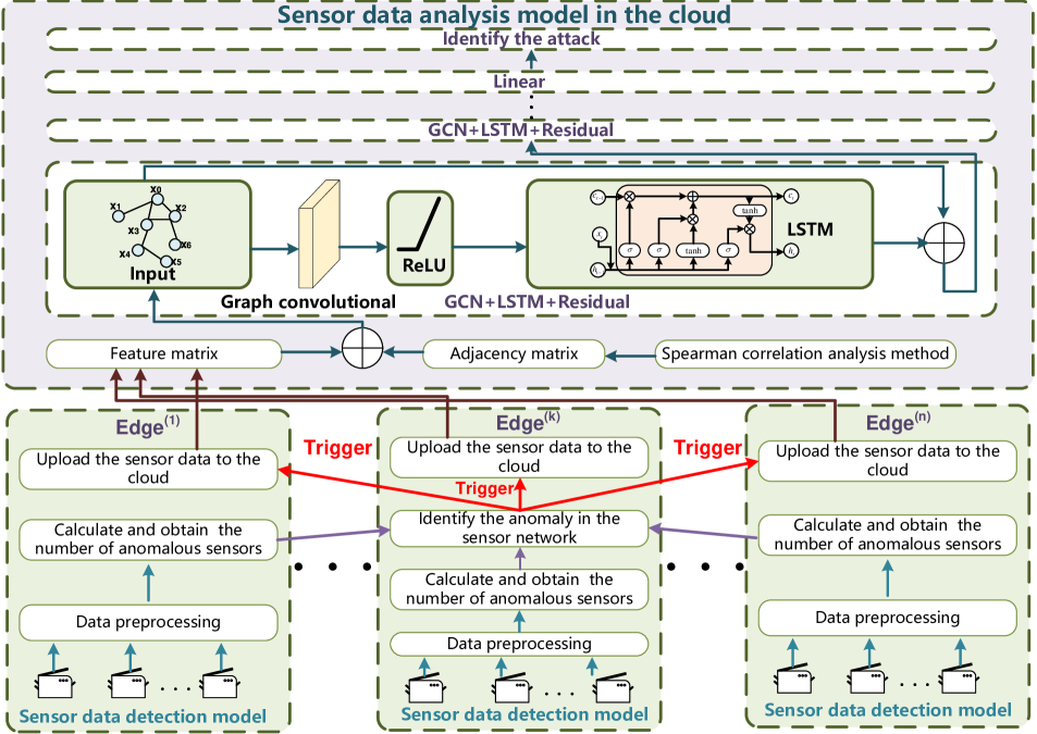
Figure 1: The framework of the proposed hybrid anomaly detection approach

The framework of the proposed hybrid anomaly detection approach in the cloud-edge collaboration industrial sensor network is shown in Fig. 1. The edge areas are divided by function (e.g., water supply, elevated reservoir, consumer tank). The sensor data detection model is deployed at the edge, which can identify whether the value of each sensor at this edge is abnormal, and calculate the number of anomalous sensors at the edge. Then the number of anomalous sensor data in each edge will be transmitted to the $Edge^{(k)}$ and the anomalous sensor data in the whole sensor network can be counted, and if it exceeds the sensitivity coefficient $e$, the sensor network will be identified as abnormal. And the corresponding original sensor data in each edge will be uploaded to the cloud for further analysis. The sensor data analysis model based on GCRL in the cloud consists of the Spearman correlation analysis algorithm, GCN, LSTM and residual algorithm. The adjacency matrix of the sensor network can be built using the Spearman correlation analysis algorithm. The sensor data analysis model can identify the attack with high precision and recall. The algorithm of the proposed hybrid anomaly detection approach is given in Algorithm 2, where $layer$ is the number of layers of the sensor data analysis model based on GCRL.

IV EXPERIMENTS AND NUMERICAL RESULTS

The proposed hybrid anomaly detection model is evaluated using the Water Distribution (WADI) dataset [18] compared with other classification models. Firstly, the sensor data detection model at the edge is evaluated, filtering massive normal data and uploading the anomalous data. Then, the adjacency matrix of the industrial sensor network is constructed using the Spearman correlation analysis algorithm. Moreover, the proposed hybrid model based on Gaussian, Bayesian and GCRL (G-GCRL) is evaluated with different parameter settings. Finally, the proposed hybrid model is compared with other state-of-art models.

Algorithm 2 Hybrid anomaly detection approach in the cloud-edge collaboration industrial sensor network

Input: the training set, real-time original sensor data $x_{r,i,t},r=(1,2,\cdots,k),i=(1,2,\cdots,m_{r})$

Output: attack type

1:  Obtain the normal and abnormal PDF for each sensor using the equations (1)-(4)

2:  Calculating the adjacency matrix A using the training set

3:  Train classification algorithm based on GCRL using the training set.

4:  Real-time original sensor data is collected at the edges

5:  if the sensor network is identified as normal using the sensor detection model at the edges then

6:     Jump $Step\;4$

7:  else

8:     upload the original sensor data $F_{t}$ to the cloud

9:     $A$ and $F_{t}$ are the input of the GCRL model

10:     for $l\leftarrow 1$ to $layer$ do do

11:        Extract the spatial features using the equation (10)

12:        Process the temporal features using the equation (11)

13:        Sum the results of $Step\;11$ and $Step\;12$ using the equation (12)

14:     end for

15:     Obtain the attack type

16:  end if

17:  Jump Step 4

The experiments are carried out based on the workstation that is equipped with NIVIDA RTX 3090 GPU, Pytorch 1.5, 64GB memory, Intel(R) Core (TM) i9-9820X CPU. The models are trained using the Adam optimizer with the learning rate of 0.01 and the significance level $\alpha=0.05$. Here, $layer=5$ and the activation function is ReLu.

IV-A Dataset

The WADI testbed is a distribution system consisting of many pipelines spanning across a large area, forming a storage and distribution network, realistic and complete water treatment. Researchers can launch possible cyber-physical and physical attacks on the WADI testbed. The WADI dataset consists of 14 types of attack data and 14-day continuous normal operation data. During the normal and attack data collection, all actuator-sensor data were collected. There are 60 actuators and 67 sensors in the WADI dataset. And the sampling period is 1s, representing 127 features that can be collected with the sampling rate of 1 s. The details of training data and testing data are shown in Table I and Table II:

TABLE I: The Details of 2-classification WADI dataset

Item	Training	Testing
normal	129210	33614
Abnormal	7843	1967

TABLE II: The Details of 15-classification WADI dataset

Item	Training	Testing
normal	129210	33614
#attack 1	1188	298
#attack 2	461	116
#attack 3	1383	346
#attack 4	670	168
#attack 5	522	131
#attack 6	548	138
#attack 7	455	114
#attack 8	70	18
#attack 9	636	159
#attack 10	527	132
#attack 11	279	70
#attack 12	153	39
#attack 13	455	114
#attack 14	496	124

IV-B Sensor data detection model at the edge

In this part, the sensor data detection model based on Gaussian and Bayesian algorithms at the edge will be evaluated using the 2-classification WADI dataset. Here, $B$ is selected as 10, representing that the sensor data is detected every 10 seconds. The evaluation metrics are shown as follows:

$$FNR=\frac{FN}{TP+FN}$$ (13)

$$k_{-}times=TP+FP$$ (14)

$$\overline{Time}=\frac{1}{n}\sum Time$$ (15)

$$RTL=\left(N_{ab+no}-k_{-}times*B\right)*N_{-}sensors$$ (16)

where True Positive (TP) represents the number of abnormal samples classified as abnormal correctly. False Negative (FN) is the number of abnormal samples classified as normal incorrectly. False Positive (FP) represents the number of normal samples classified as abnormal incorrectly. $k_{-}times$ is the times of uploading the anomalous data to the cloud. $RTL$ represents the number of filtered sensor data by the sensor data detection model, which is corresponding to the traffic load. $N_{ab+no}$ is the number of samples in the testing set. $N_{-}sensors$ is the number of sensors in the sensor network. $\overline{Time}$ is the mean time of processing an aggregated sample.

This work also considers the influence of sensitivity coefficient $e$ on the detection results. The numerical results are presented in TABLE III.

TABLE III: The Results of The Sensor Data Detection Model

$e$	$TP$	$FP$	$FNR$	$k_{-}times$	$RTL$	$\overline{Time}$
15	196	3361	0	3557	255397	22.32ms
20	196	3037	0	3233	412877	22.21ms
21	196	2464	0	2660	1140587	22.19ms
22	196	1374	0	1570	2537587	22.86ms
23	196	1012	0	1208	2984627	23.30ms
24	196	843	0	1039	3199257	22.94ms
25	196	759	0	955	3305937	22.77ms
26	196	721	0	917	3354197	22.98ms
27	196	663	0	859	3427857	22.83ms
28	193	538	1.53%	731	3590417	22.77ms
29	167	243	14.79%	410	4466717	22.49ms
31	111	0	43.37%	111	4504690	22.21ms
33	19	0	90.31%	19	45134657	22.49ms

In TABLE III, the time window for sensor data collection is 10s, and $\overline{Time}$ is about 22ms. Therefore, the sensor data detection model at the edge meets the requirement of real-time. With the increase of $e$, $TP$, $FP$, and $k_{-}times$ will decrease but $FNR$ and $RTL$ will increase. Therefore, more anomalous sensor data will be detected if $e$ is small, but more normal sensor data will be incorrectly classified as abnormal and $RTL$ will be small, leading to heavy traffic load. The increase in traffic load may lead to many serious problems (loss of control commands, packet corruption) in ICS. For the sensor data detection model at the edge, we expect the traffic load can be smaller, i.e., $RTL$ should be bigger and the $FNR$ must be zero. Each anomalous sample is critical for analyzing the whole attack event e.g., attack path construction and situational awareness, so all the anomalous sensor data must be uploaded to the cloud, even to increase the traffic load. Therefore, we can consider the $e$=27 is a turning point, because the $FNR$ is not zero when $e$ is more than 27. Moreover, the $RTL$ when $e$=22 is about twice as much as $RTL$ when $e$=21, so we consider the $e$=22 is a turning point. Different values of $e$ can affect the classification results of the sensor data analysis model in the cloud. Therefore, we consider $e$ is 22, 23, 24, 25, 26, 27 for further analysis in the following experiments and finally select the best parameter which can make the proposed model perform best. Furthermore, we can reduce the amount of sensor data uploaded to the cloud by millions, using the proposed cloud-edge collaborative framework.

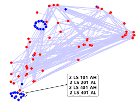
(a) $p$ is 0.45

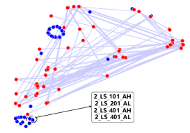
(b) $p$ is 0.55

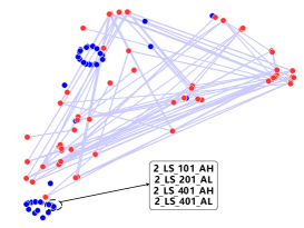
(c) $p$ is 0.65

Figure 2: The sensor data correlation graphs

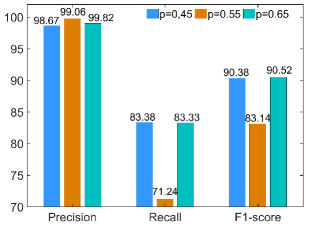
(a) $e$ is 22

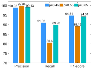
(b) $e$ is 23

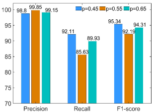
(c) $e$ is 24

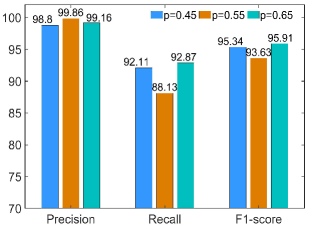
(d) $e$ is 25

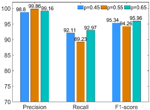
(e) $e$ is 26

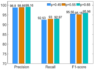
(f) $e$ is 27

Figure 3: Comparison of different parameter settings

IV-C Sensor data analysis model in the cloud

The sensor data analysis model in the cloud based on GCRL consists of the Spearman correlation coefficient algorithm, GCN, LSTM and Residual method. The sensor data uploaded by the detection model at the edges will be analyzed and the attack can be identified precisely. Firstly, the adjacency matrix $A$ can be built using the Spearman correlation analysis algorithm with the training set in TABLE I. To visualize the adjacency matrix $A$, we use the corresponding sensor data correlation graph. The sensor data correlation graphs built using the Spearman correlation coefficient algorithm are shown in Fig. 2. Each point represents a sensor, and the coordinates are calculated using the t-distributed stochastic neighbor embedding (TSNE) [33]. If one sensor is associated with other sensors, the sensor is a red point, while the blue points are the opposite. The edge represents that there exists a correlation between the two sensors. The edges in Fig. 2(a) are denser than that in Fig. 2(b) and Fig. 2(c). Therefore, we can conclude that the sensor data correlation graphs are different when $p$ is different, which will affect the final classification results.

Then, the proposed hybrid model is evaluated with different parameter settings. Here, the parameter $e$ is 22, 23, 24, 25, 26 or 27 and the parameter $p$ is 0.45, 0.55 or 0.65. In the experiments, the abnormal training data is resampled for 10 times due to the imbalance between the number of normal training data and abnormal training data.

In the experiments, the following metrics in equations (17)- (19) are used to evaluate the proposed solution:

$$\text{ Precision }=\frac{TP}{TP+FP}$$ (17)

$$\text{ Recall }=\frac{TP}{TP+FN}$$ (18)

$$\text{ F1-score }=\frac{2*\text{ Precision }*\text{ Recall }}{\text{ Precision }+\text{ Recall }}$$ (19)

The comparison results are shown in Fig. 3(a) - Fig. 3(f). F1-score is the parameter that can balance Precision and Recall, so we consider selecting the parameters that maximize the F1-score in this paper. The Precision is always higher than 98% with different parameter settings. However, the Recall fluctuates from 71.24% to 93%. Moreover, the F1-score 95.96% is the highest when $p$=0.65 if $e$=26 or $e$=27. But the traffic load is smaller when $e$=27, compared with $e$=26. Therefore, we select $p$=0.65 and $e$=27 as the parameters of G-GCRL.

Moreover, we also compare the proposed hybrid model with GCN and GCRL to validate the proposed cloud-edge collaborative framework. The comparison results are shown in Fig. 4. The Precision is almost the same, but the Recall and F1-score are very different in this three models. The Recall and F1-score of GCN are 50.44% and 66.58%, respectively. However, the Recall and F1-score of the G-GCRL are the highest, which is 49.49% and 25.72% higher than that of GCRL, respectively.

Further, the performance of the proposed hybrid model is evaluated against ten different anomaly detection models, including PCA [24], KNN [35]. FB [34], AE [29], MAD-GAN [14], LSTM-VAE [25] and the following models:

DAGMM [28]: Deep Autoencoding Gaussian model joints deep Autoencoders and Gaussian Mixture Model to identify anomalous data.

AQADF [18]: The automatic Quasi-periodic time series anomaly detection framework (AQADF) consists of a clustering algorithm and a hybrid LSTM-CNN model with an attention mechanism, which can identify the anomalous data.

GDN [9]: Graph Deviation Network (GDN) approach can learn a graph of relationships between sensors, and calculates deviations from these patterns.

GTA [21]: Graph Learning with Transformer for Anomaly detection (GTA) involves automatically learning a graph structure, and extracting temporal features using a transformer and graph convolution.

TABLE IV: The Results of Different Models with 2-classification Dataset

Model	Precision(%)	Recall(%)	F1-score
PCA	39.53	53.63	0.10
KNN	7.76	7.75	0.08
FB	8.60	8.60	0.09
AE	34.35	34.35	0.34
MAD-GAN	41.44	33.92	0.37
DAGMM	54.44	26.99	0.36
LSTM-VAE	87.79	14.45	0.25
ARADF	89.15	20.34	0.42
GDN	97.5	40.19	0.57
GTA	83.91	83.61	0.84
G-GCRL	99.16	92.97	0.96

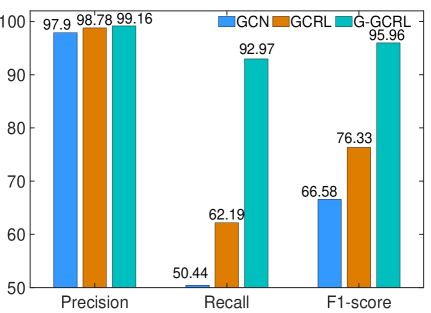
Figure 4: Comparison of different anomaly detection models

The comparison results of different models are shown in TABLE IV. The best performance is highlighted in bold and the second-best with underlines. Our proposed hybrid anomaly detection model based on G-GCRL significantly outperforms all other models for the same dataset with the performance of Precision, Recall and F1-score up to 99.16%, 92.97% and 0.96, respectively. In addition, compared to the second-best model, G-GCRL can achieve an overall 11.19% and 14.29% improvement for Recall and F1-score, respectively.

Further, the proposed G-GCRL model is assessed using the dataset in TABLE II, compared with the ARADF and GCN. The accuracy of each attack type is used as the following metric.

$$EACC_{type_{j}}=\frac{TP_{type_{j}}}{number_{type_{j}}}$$ (20)

where $TP_{type_{j}}$ is the number of correctly classified data in $attack\;j$ dataset. $number_{type_{j}}$ is the number of data in $attack\;j$ dataset. The comparison results are shown in Fig. 5.

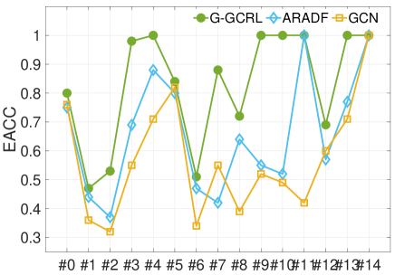
Figure 5: The comparison results of multi-classification

In Fig. 5, #0 represents the normal and #1 to #14 represent $attack$ 1 to $attack$ 14, respectively. The accuracy of each attack of the G-GCRL model is always higher than that of the other models. Moreover, if the classifier is the G-GCRL model, the accuracy of $attack$ 4, 9, 10, 11, 13 and 14 is almost 100%, respectively. However, the accuracy of $attack$ 1, 2 and 6 are lower than 0.6 in the 3 models, indicating that the 3 attacks are hard to be identified.

V Conclusions

This paper proposes a hybrid anomaly detection approach deployed in cloud-edge collaboration industrial sensor networks, consisting of sensor data detection models deployed at the edges and a sensor data analysis model deployed in the cloud. The sensor data detection model can detect the anomalous sensor data and then upload them to the cloud for further analysis, filtering massive normal sensor data and making traffic load smaller. The sensor data analysis model can efficiently extract temporal and spatial features and identify the attack precisely. The benchmark dataset WADI is used for evaluation compared with other baseline models. The numerical results show that our proposed approach can achieve an overall 11.19% increase in Recall and an impressive 14.29% improvement in F1-score, compared with the existing baseline models.

For future research, more advanced sensor data anomaly detection models need to be considered. Furthermore, the method of building the sensor data correlation graph can also be investigated for further analysis. Also, the performance of the proposed approach needs to be extensively assessed in the presence of advanced persistent threat (APT) attacks.

References

- [1] Internet of Things, IL Brief, Int. Renew. Energy Agency, Abu Dhabi, UAE, 2019.
- [2] Strategic Principles for Securing the Internet of Things (IoT), U.S. Department of Homeland Security, 2016.
- [3] F. Salvadori et al., ”Monitoring in Industrial Systems Using Wireless Sensor Network With Dynamic Power Management,” in IEEE Transactions on Instrumentation and Measurement, vol. 58, no. 9, pp. 3104-3111, Sept. 2009.
- [4] H. Y. Teh, K. I. -K. Wang and A. W. Kempa-Liehr, “Expect the Unexpected: Unsupervised Feature Selection for Automated Sensor Anomaly Detection,” in IEEE Sensors Journal, vol. 21, no. 16, pp. 18033-18046, Aug. 2021.
- [5] Y. Xu and A. Helal, “Scalable Cloud–Sensor Architecture for the Internet of Things,” in IEEE Internet of Things Journal, vol. 3, no. 3, pp. 285-298, June 2016.
- [6] F. V. Jensen, An Introduction to Bayesian Networks, vol. 210. London, U.K.: UCL Press, 1996.
- [7] F. Wang, S. Wu, K. Wang and X. Hu, “Energy-Efficient Clustering Using Correlation and Random Update Based on Data Change Rate for Wireless Sensor Networks,” in IEEE Sensors Journal, vol. 16, no. 13, pp. 5471-5480, July. 2016.
- [8] T. N. Kipf and M. Welling, “Semi-supervised classification with graph convolutional networks,” in 5th International Conference on Learning Representations, 2017.
- [9] Deng and B. Hooi, “Graph neural network-based anomaly detection in multivariate time series,” in Proceedings of the 35th AAAI Conference on Artificial Intelligence, 2021.
- [10] G. W. Corder and D. I. Foreman, Nonparametric Statistics: A Step-by-Step Approach, 2nd ed. Hoboken, NJ, USA: Wiley, 2014.
- [11] S. Hochreiter and J. Schmidhuber, “Long short-term memory,” Neural Comput., vol. 9, no. 8, pp. 1735–1780, 1997.
- [12] K. He, X. Zhang, S. Ren, and J. Sun, “Deep residual learning for image recognition,” in Proc. IEEE Conf. Comput. Vis. Pattern Recognit., Las Vegas, NE, USA, pp. 770–778, Jun. 2016.
- [13] M. Shyu, S. Chen, S. Kanoksri, and L. Chang, “A Novel Anomaly Detection Scheme Based on Principal Component Classifier,” in Proceedings of International Conference on Data Mining, 2003.
- [14] R. Sharififi and R. Langari, “Nonlinear sensor fault diagnosis using mixture of probabilistic PCA models,” in Mech. Syst. Signal Process., vol. 85, pp. 638–650, Feb. 2017.
- [15] R. Jiang, H. Fei, and J. Huan, “A family of joint sparse PCA algorithms for anomaly localization in network data streams,” IEEE Trans. Knowl. Data Eng., vol. 25, no. 11, pp. 2421–2433, Nov. 2013.
- [16] W. Hao, P. Yao, T. Yang and Q. Yang, ”Industrial cyber-physical system defense resource allocation using distributed anomaly detection,” in IEEE Internet of Things Journal.
- [17] D. Huang, X. Shi and W. Zhang, “False Data Injection Attack Detection for Industrial Control Systems Based on Both Time- and Frequency-Domain Analysis of Sensor Data,” in IEEE Internet of Things Journal, vol. 8, no. 1, pp. 585-595, Jan. 2021.
- [18] D. Li, D. Chen, B. Jin, L. Shi, J. Goh, and S. Ng, “MAD-GAN: multivariate anomaly detection for time series data with generative adversarial networks,” in 28th International Conference on Artificial Neural Networks, ser. Lecture Notes in Computer Science, vol. 11730. Springer, 2019, pp. 703–716.
- [19] Y. -H. Nho, S. Ryu and D. -S. Kwon, “UI-GAN: Generative Adversarial Network-Based Anomaly Detection Using User Initial Information for Wearable Devices,” in IEEE Sensors Journal, vol. 21, no. 8, pp. 9949-9958, April. 2021.
- [20] Y. Liu et al., “Deep Anomaly Detection for Time-Series Data in Industrial IoT: A Communication-Efficient On-Device Federated Learning Approach” in IEEE Internet of Things Journal, vol. 8, no. 8, pp. 6348-6358, April. 2021.
- [21] F. Liu et al., “Anomaly Detection in Quasi-Periodic Time Series based on Automatic Data Segmentation and Attentional LSTM-CNN,” in IEEE Transactions on Knowledge and Data Engineering.
- [22] C. Hwang and T. Lee, “E-SFD: Explainable Sensor Fault Detection in the ICS Anomaly Detection System,” in IEEE Access, vol. 9, pp. 140470-140486, 2021.
- [23] D. Park, Y. Hoshi and C. C. Kemp, “A Multimodal Anomaly Detector for Robot-Assisted Feeding Using an LSTM-Based Variational Autoencoder,” in IEEE Robotics and Automation Letters, vol. 3, no. 3, pp. 1544-1551, July 2018
- [24] M. S. S. Garmaroodi, F. Farivar, M. S. Haghighi, M. A. Shoorehdeli and A. Jolfaei, “Detection of Anomalies in Industrial IoT Systems by Data Mining: Study of CHRIST Osmotron Water Purification System,” in IEEE Internet of Things Journal, vol. 8, no. 13, pp. 10280-10287, July. 2021.
- [25] M. Sakurada and T. Yairi. “Anomaly Detection Using Autoencoders with Nonlinear Dimensionality Reduction,” in Proceedings of the MLSDA 2014 2nd Workshop on Machine Learning for Sensory Data Analysis (MLSDA’14).
- [26] C. C. Aggarwal, “Data mining,” in Outlier Analysis. Springer, 2017, pp. 237–263.
- [27] Deng and B. Hooi, “Graph neural network-based anomaly detection in multivariate time series,” in Proceedings of the 35th AAAI Conference on Artificial Intelligence, 2021.
- [28] Z. Chen, D. Chen, X. Zhang, Z. Yuan and X. Cheng, “Learning Graph Structures with Transformer for Multivariate Time Series Anomaly Detection in IoT,” in IEEE Internet of Things Journal.
- [29] D. Wu, Z. Jiang, X. Xie, X. Wei, W. Yu and R. Li, “LSTM Learning With Bayesian and Gaussian Processing for Anomaly Detection in Industrial IoT,” in IEEE Transactions on Industrial Informatics,” vol. 16, no. 8, pp. 5244-5253, Aug. 2020.
- [30] A. Saci, A. Al-Dweik and A. Shami, “Autocorrelation Integrated Gaussian Based Anomaly Detection using Sensory Data in Industrial Manufacturing,” in IEEE Sensors Journal, vol. 21, no. 7, pp. 9231-9241, April. 2021.
- [31] B. Zong, Q. Song, M. R. Min, W. Cheng, C. Lumezanu, D. Cho, and H. Chen, “Deep autoencoding Gaussian mixture model for unsupervised anomaly detection,” in Proc. Int. Conf. Learn. Represent. (ICLR), 2018, pp. 1–19.
- [32] R. A. Fisher, “Statistical methods for research workers,” in Breakthroughs in Statistics. New York, NY, USA: Springer, 1992, pp. 66–70.
- [33] L. van der Maaten, , G. Hinton (2008), “Viualizing data using t-SNE,” in Journal of Machine Learning Research, vol.9, pp. 2579-2605, Nov. 2008.
- [34] A. Lazarevic and V. Kumar, “Feature Bagging for Outlier Detection,” in Proc. ACM SIGKDD, pp. 157-166, 2005.
- [35] F. Angiulli and C. Pizzuti, “Fast Outlier Detection in High Dimensional Spaces,” in Proc. Int’l Conf. Principles of Data Mining and Knowledge Discovery (PKDD ’02), pp. 15-26, 2002.