Singularity-Avoiding Multi-Dimensional Root-Finder

Abstract

We proposed in this paper a new method, which we named the W4 method, to solve nonlinear equation systems. It may be regarded as an extension of the Newton-Raphson (NR) method to be used when the method fails. Indeed our method can be applied not only to ordinary problems with non-singular Jacobian matrices but also to problems with singular Jacobians, which essentially all previous methods that employ the inversion of the Jacobian matrix have failed to solve. In this article, we demonstrate that (i) our new scheme can define a non-singular iteration map even for those problems by utilizing the singular value decomposition, (ii) a series of vectors in the new iteration map converges to the right solution under a certain condition, (iii) the standard two-dimensional problems in the literature that no single method proposed so far has been able to solve completely are all solved by our new method.

1 Introduction

The root-finding of functions is one of the most important problems in computational science and engineering. It is a nontrivial task, however, to numerically find the root of a system of nonlinear equations:

$$\bm{F}(\bm{x})=\mathbf{0},$$ (1)

where $\bm{x}\in\mathbb{R}^{N}$, $N\in\mathbb{Z}$ and $\bm{F}:\mathbb{R}^{N}\rightarrow\mathbb{R}^{N}$. Although the single-variable problem is rather simple, it becomes particularly difficult when $N>1$. The Newton-Raphson (NR) method may be the first choice, since it is well-known to give a solution as long as the initial guess is sufficiently close to the solution[1, 2]. Another advantage for the NR method is its quadratic convergence to the solution if the Jacobian matrix for the system of nonlinear equations (1) is non-singular. Many attempts done so far to further accelerate the convergence: Halley’s and Householder’s methods for single-variable problems[3] and Ramos& Monteiro’s method for multi-variable problems to mention a few [4, 5].

There are demerits in the NR method, though. Very heavy computational cost in the inversion of Jacobian matrix for large system dimensions is one of them: the operation number scales as $\mathcal{O}\left(N^{3}\right)$. Many efforts have been successfully made to reduce the cost to $\mathcal{O}\left(N^{2}\right)$[6, 2]. Another common disadvantage for the NR and other quasi-Newton methods is the strong dependence of convergence on the initial condition for iteration. It is crucial indeed for whether the iteration can reach a solution or not. We commonly come across situations, in which the iteration is simply divergent or suffers from permanent oscillations. Recently, we proposed a new method referred to as the W4 method to circumvent such difficulties. We have shown that the W4 method is able to obtain a solution even if the NR method fails[7]. In fact, the W4 method has been successfully applied to some physical problems already[8, 9, 10].

The existence of singularity in the Jacobian matrix is a different issue. If the Jacobian matrix is singular at the solution, the convergence is slowed down severely and we are required to take some measure to reaccelerate it[11, 12, 13]. If the Jacobian is singular either at the initial guess or at intermediate steps in the iteration, the problem is much more serious, since one cannot invert the Jacobian matrix and hence cannot define the iteration map to the next step. In the existing multi-variable root finders, to the best of our knowledge, one needs to somehow modify (normally by hand) the initial guess or the intermediate results in such situations. In this article, we try to deal with this difficulty in the framework of the W4 method and establish the foundation of a globally convergent multi-variable root-finder. We hence focus on two dimensional problems with singular Jacobian matrices in this article.

The paper is organized as follows. We first present our new scheme to find roots of nonlinear equation systems in the framework of the W4 method in Sec. 2, clarifying how the singular nature of the associated Jacobian matrix is handled. We also show that our method is applicable to ordinary non-singular problems as well. In Sec. 3, we demonstrate the capabilities of the new method by applying it to the standard test problems in the literature comparing the results with those of other methods. Finally, we summarize our findings and comment on future prospects in Sec. 4.

2 Singularity Avoidance with the W4 method

In this paper, we consider two dimensional nonlinear equations, which are expressed in general as

$$\bm{F}(x,y)\equiv\begin{pmatrix}f_{x}(x,y)\\ f_{y}(x,y)\end{pmatrix}=\bm{0}.$$ (2)

For iterative solvers, such as the Newton-Raphson method and the W4 method, it is normally necessary to calculate the Jacobian matrix associated with the system of equations:

$$J=\begin{pmatrix}\frac{\partial f_{x}}{\partial x}&\frac{\partial f_{x}}{\partial y}\\ \frac{\partial f_{y}}{\partial x}&\frac{\partial f_{y}}{\partial y}\end{pmatrix}.$$ (3)

We call the Jacobian singular when $\det J=0$. In our previous article [7], we proposed a new multi-dimensional root-finding scheme, the W4 method, and demonstrated that it can solve some problems that the Newton-Raphson method fails to solve. As shown, the W4 method with the UL [7] or the LH decomposition [8] has a tendency to leap over singularities by inertia. We observed, however, that even the W4 method is stalled sometimes, particularly when the initial guess has a singular Jacobian. The new method we propose in this article solves this problem. Below we explain how we define the iteration map in this method for such situations, i.e., when a singularity is encountered either at the initial step or at some intermediate steps in the iteration.

2.1 Eigendecomposition

At first, we look at some relevant properties of the Jacobian matrix that may be singular. Suppose we have a $2\times 2$ real matrix $A$. The two eigenvalues for this matrix $A$ are given as

$$\lambda_{\pm}=\frac{1}{2}\left(\alpha\pm\sqrt{\alpha^{2}-4\beta}\right),$$ (4)

where we define $\alpha:=\mathrm{tr}A$ and $\beta:=\det A$. Assuming eigenvectors $\bm{w}_{\pm}$ for $\lambda_{\pm}$, respectively, we decompose the Jacobian into

$$A=P\Lambda P^{-1}=\begin{pmatrix}\bm{w}_{+}&\bm{w}_{-}\end{pmatrix}\begin{pmatrix}\lambda_{+}&0\\ 0&\lambda_{-}\end{pmatrix}\begin{pmatrix}\bm{w}_{+}^{T}\\ \bm{w}_{-}^{T}\end{pmatrix}.$$ (5)

Note that the eigenvalues are generally complex unless the Jacobian is symmetric.

For a singular Jacobian $J$, one eigenvalue is $\lambda_{+}=\alpha$ and the other is $\lambda_{-}=0$ since $\beta=\det J=0$ by definition from Eq. (4). Then the singular Jacobian can be rewritten as

$$J=\lambda_{+}\bm{w}_{+}\bm{w}_{+}^{T}.$$ (6)

2.2 Singular Value Decomposition

As mentioned above, there may not exist all the eigenvectors. We hence consider the singular value decomposition of the Jacobian. The following equations:

$$J\bm{v}=\sigma\bm{u},$$ (7)

$$J^{T}\bm{u}=\sigma\bm{v},$$ (8)

yield

$$J^{T}J\bm{v}=\sigma^{2}\bm{v},$$ (9)

$$JJ^{T}\bm{u}=\sigma^{2}\bm{u}.$$ (10)

In these equations, $\sigma$’s are called the singular values of $J$. Since they are defined as the positive square root of $\sigma^{2}$, the eigenvalues of positive-semidefinite symmetric matrix of $J^{T}J$ or $JJ^{T}$, the corresponding vectors, $\bm{u}$ and $\bm{v}$, always exist.

Lemma 1.

Suppose a $2\times 2$ Jacobian matrix is singular, then one of the singular values is at least zero.

Proof.

When the Jacobian $J$ is singular, i.e., $\det J=0$, we obtain $\beta=\det A=\det(J^{T}J)=(\det J)^{2}=0$ for the matrix $A=J^{T}J$. Then from Eq. (4), the square of the smaller singular value is given as $\sigma^{2}_{-}=(\alpha-\sqrt{\alpha^{2}-4\beta})/2=0$. ∎

Let $U=[\bm{u}_{+}\ \bm{u}_{-}]$ and $V=[\bm{v}_{+}\ \bm{v}_{-}]$ be the orthogonal matrices given by the two independent eigenvectors associated with $JJ^{T}$ and $J^{T}J$, respectively, and $\Sigma=\mathrm{diag}[\sigma_{+},\ \sigma_{-}]$ be the diagonal matrix. The Jacobian can be decomposed as

$$J=U\Sigma V^{-1}=\begin{pmatrix}\bm{u}_{+}&\bm{u}_{-}\end{pmatrix}\begin{pmatrix}\sigma_{+}&0\\ 0&\sigma_{-}\end{pmatrix}\begin{pmatrix}\bm{v}_{+}^{T}\\ \bm{v}_{-}^{T}\end{pmatrix},$$ (11)

which is the singular value decomposition of $J$.

Lemma 2.

Suppose a $2\times 2$ Jacobian is singular, then it can be expressed only by the right-singular and left-singular vectors, $\bm{v}_{+}$ and $\bm{u}_{+}$, which correspond to the larger singular value $\sigma_{+}$.

Proof.

Since $\sigma_{-}=0$, Eq. (11) yields $J=\sigma_{+}\bm{u}_{+}\bm{v}_{+}^{T}$. ∎

Note that, in general, the singular values $\sigma$ differ from the eigenvalues $\lambda$ and they coincide with each other if the Jacobian is symmetric $J=J^{T}$.

2.3 W4 with singular value decomposition

The generic form of the iteration map of the W4 method for variable $\bm{x}^{(n)}$ and auxiliary variable $\bm{p}^{(n)}$ at the $n$-step is given as

$$\bm{x}^{(n+1)} =\bm{x}^{(n)}+\Delta\tau X\bm{p}^{(n)},$$ (12a)

$$\bm{p}^{(n+1)} =\left(1-2\Delta\tau\right)\bm{p}^{(n)}-\Delta\tau Y\bm{F}(\bm{x}^{(n)}),$$ (12b)

where $X$ and $Y$ are preconditioner matrices, which we can choose at our disposal in principle. Linearizing the above nonlinear map at the solution ($\bm{x}=\bm{x}^{*}$ and $\bm{p}=\bm{0})$ and introducing the errors as $\bm{e}_{x}^{(n)}:=\bm{x}^{*}-\bm{x}^{(n)}$ and $\bm{e}_{p}^{(n)}:=\bm{0}-\bm{p}^{(n)}$, we obtain the error propagation equations:

$$\bm{e}_{x}^{(n+1)}= \bm{e}_{x}^{(n)}-X\Delta\tau\bm{e}_{p}^{(n)},$$ (13a)

$$\bm{e}_{p}^{(n+1)}= \left(1-2\Delta\tau\right)\bm{e}_{p}^{(n)}+YJ\Delta\tau\bm{e}_{x}^{(n)},$$ (13b)

which are rewritten as

$$\bm{e}_{z}^{(n+1)}=W\bm{e}_{z}^{(n)},\quad\bm{e}_{z}^{(n)}:=\begin{pmatrix}\bm{e}_{x}^{(n)}\\ \bm{e}_{p}^{(n)}\end{pmatrix},\quad W:=\begin{bmatrix}I&-\Delta\tau X\\ \Delta\tau YJ&(1-2\Delta\tau)I\end{bmatrix},$$ (14)

where $I$ denotes the $N\times N$ identity matrix, with $N$ being the number of nonlinear equations.

Lemma 3.

Suppose there exists a complete set of eigenvectors $\bm{v}_{i}\in\mathbb{R}^{2N}$ of the matrix $W$ in Eq. (14) and let $Q$ be a $2N\times 2N$ matrix composed of $\bm{v}_{i}$ and $d_{i}$ be the eigenvalues corresponding to $\bm{v}_{i}$, then the norm of the error vector always decreases if $|d_{max}|<1$ for the maximum eigenvector $d_{max}$.

Proof.

The matrix $W$ can be decomposed as $W=Q^{-1}DQ$ in terms of the matrix $Q:=[\bm{v}_{1}\bm{v}_{2}\cdots\bm{v}_{2N}]$ and the diagonal matrix $D:=\mathrm{diag}[d_{1},d_{2},\cdots,d_{2N}]$. Then the error propagates from the $n$-step to the $(n+1)$-step as

$$\bm{e}^{(n+1)}_{z}=W\bm{e}^{(n)}_{z}=Q^{-1}DQ\bm{e}^{(n)}_{z}.$$ (15)

Defining the auxiliary vector $\bm{q}:=Q\bm{e}^{(n)}_{z}$ for notational convenience, we evaluate the norm of the error at the $(n+1)$-step:

$$\mid\bm{e}^{(n+1)}_{z}\mid^{2} = \left(Q^{-1}DQ\bm{e}^{(n)}_{z}\right)^{T}Q^{-1}DQ\bm{e}^{(n)}_{z}=\bm{q}^{T}D^{2}\bm{q}=\sum_{i=1}^{2N}d_{i}^{2}q_{i}^{2}$$ (16)

$$< \sum_{i=1}^{2N}q_{i}^{2}=\mid\bm{q}\mid^{2}=\mid Q\bm{e}^{(n)}_{z}\mid^{2}=\mid\bm{e}^{(n)}_{z}\mid^{2},$$

where we used $|d_{i}|<1$ to derive the inequality and $Q^{T}=Q^{-1}$ to obtain the last equality. ∎

In the framework o the W4 method, the eigenvalues of the matrix $W$ in Eq. (14) are cruicially important, which are obtained from the characteristic polynomial:

$$\det\left[W-d_{W}I\right]=\det\left[(1-d_{W})(1-2\Delta\tau-d_{W})I+\Delta\tau^{2}YJX\right]=0.$$ (17)

Definition 1.

We define the W4SV method as the following choice of matrices $X$ and $Y$ in Eqs. (12a) and (12b): $X=V$ and $Y=\hat{\Sigma}^{-1}U^{-1}$, where $U,V$ and $\hat{\Sigma}$ are the matrices in the singular decomposition of Jacobian $J$ and we define $\hat{\Sigma}^{-1}$ as

$$\hat{\Sigma}^{-1}=\begin{cases}\mathrm{diag}\left[\sigma_{+}^{-1},\sigma_{-}^{-1}\right]&(\sigma_{-}\neq 0),\\ \mathrm{diag}\left[\sigma_{+}^{-1},1\right]&(\sigma_{-}=0).\end{cases}$$ (18)

Proposition 1.

Suppose all singular values of Jacobian $J$ in the two dimensional problems are nonzero, then the W4SV map with $0<\Delta\tau<1$ yields a series of vectors $\bm{x}^{(n)}$ that converge to a solution if the initial condition is sufficiently close to the solution.

Proof.

Since the Jacobian matrix is decomposed as $J=U\Sigma V^{-1}$, we have $\hat{\Sigma}^{-1}U^{-1}JV=I$

when all the singular values are nonvanishing. Then the eigenvalues of the matrix $W$ in Eq. (14) can be calculated from Eq. (17):

$$\det\left[W-d_{W}I\right]=\det\left[(1-d_{W})(1-2\Delta\tau-d_{W})I+\Delta\tau^{2}I\right]=\det\left[\left(1-\Delta\tau-d_{W}\right)^{2}I\right]=0$$ (19)

as $d_{W}=1-\Delta\tau$. It is obvious that $|d_{W}|<1$ for $0<\Delta\tau<1$. If the initial condition is sufficiently close to the solution, the linearized equation (14) is valid and the error should decrease monotonically and the iteration will converge to the solution. ∎

Lemma 4.

Suppose one of the singular values of a $2\times 2$ singular Jacobian matrix is vanishing, then one of the eigenvalues of the matrix $W$ for the W4SV map is unity.

Proof.

Since the singular Jacobian is written as $J=\sigma_{+}\bm{u}_{+}\bm{v}_{+}^{T}$, the matrix $YJX$ is calculated as follows:

$$YJX = \hat{\Sigma}^{-1}U^{-1}JV=\begin{pmatrix}\sigma_{+}^{-1}&0\\ 0&1\end{pmatrix}\begin{pmatrix}\bm{u}_{+}^{T}\\ \bm{u}_{-}^{T}\end{pmatrix}\sigma_{+}\bm{u}_{+}\bm{v}_{+}^{T}\begin{pmatrix}\bm{v}_{+}&\bm{v}_{-}\end{pmatrix}$$ (20)

$$= \begin{pmatrix}\sigma_{+}^{-1}&0\\ 0&1\end{pmatrix}\begin{pmatrix}\sigma_{+}\bm{v}_{+}^{T}\\ \bm{0}^{T}\end{pmatrix}\begin{pmatrix}\bm{v}_{+}&\bm{v}_{-}\end{pmatrix}=\begin{pmatrix}\sigma_{+}^{-1}&0\\ 0&1\end{pmatrix}\begin{pmatrix}\sigma_{+}&0\\ 0&0\end{pmatrix}=\begin{pmatrix}1&0\\ 0&0\end{pmatrix}.$$

Then the characteristic polynomial equation becomes

$$0=\det\left[W-d_{W}I\right]=\det\begin{bmatrix}(1-\Delta\tau-d_{W})^{2}&0\\ 0&(1-d_{W})(1-\Delta\tau-d_{W})\end{bmatrix}=(1-d_{W})(1-\Delta\tau-d_{W})^{3}.$$ (21)

It is now apparent that one of the eigenvalues is $d_{W}=1$ and the other is $d_{W}=1-\Delta\tau$. ∎

Proposition 2.

Suppose one of the singular values of the $2\times 2$ Jacobian matrix at the $n$-step is vanishing as in Lemma 4, then the W4SV map with $\Delta\tau=1/2$ produces an increment that is not aligned with $\bm{v}_{+}$ or $\bm{v}_{-}$ in general. Such an alignment occurs only when the angle between $\bm{F}(\bm{x}^{(n)})$ and $\bm{u}_{+}^{(n)}$ accidentally satisfies a particular relation with the angle between $\bm{v}_{+}^{(n)}$ and $\bm{v}_{+}^{(n+1)}$.

Proof.

The W4SV map with $\Delta\tau=1/2$ is given as

$$\bm{x}^{(n+1)} =\bm{x}^{(n)}+\frac{1}{2}V\bm{p}^{(n)},$$ (22a)

$$\bm{p}^{(n+1)} =-\frac{1}{2}\hat{\Sigma}^{-1}U^{-1}\bm{F}(\bm{x}^{(n)}).$$ (22b)

The increment at the $(n+1)$-step can be written as

$$\bm{x}^{(n+2)}-\bm{x}^{(n+1)} = -\frac{1}{4}V_{(n+1)}\hat{\Sigma}_{(n)}^{-1}U_{(n)}^{T}\bm{F}(\bm{x}^{(n)})=-\frac{F\cos\theta}{4\sigma_{+}^{(n)}}\bm{v}_{+}^{(n+1)}-\frac{F\sin\theta}{4}\bm{v}_{-}^{(n+1)},$$ (23)

where $\cos\theta$ is the angle between $\bm{u}_{+}^{(n)}$ and $\bm{F}(\bm{x}^{(n)})$ and $F=|\bm{F}|$ is the absolute value of vector $\bm{F}$. With the employment of the angle $\phi$ between $\bm{v}_{+}^{(n)}$ and $\bm{v}_{+}^{(n+1)}$, the right-singular vectors $\bm{v}_{+}^{(n)}$ and $\bm{v}_{-}^{(n)}$ at the $(n+1)$-step are expanded by those at the $n$-step as follows:

$$\bm{v}_{+}^{(n+1)}=\bm{v}_{+}^{(n)}\cos\phi-\bm{v}_{-}^{(n)}\sin\phi,$$

$$\bm{v}_{-}^{(n+1)}=\bm{v}_{+}^{(n)}\sin\phi+\bm{v}_{-}^{(n)}\cos\phi.$$ (24)

The increment is finally expressed by the latter vectors as

$$\bm{x}^{(n+2)}-\bm{x}^{(n+1)} = -\frac{F}{4\sigma_{+}^{(n)}}\left\{\cos\theta\cos\phi+\sigma_{+}^{(n)}\sin\theta\sin\phi\right\}\bm{v}_{+}^{(n)}+\frac{F}{4\sigma_{+}^{(n)}}\left\{\cos\theta\sin\phi-\sigma_{+}^{(n)}\sin\theta\cos\phi\right\}\bm{v}_{-}^{(n)}.$$

This indicates that the increment in the direction of $\bm{v}_{-}^{(n)}$ exists unless $\cos\phi=\cos\theta=0$ or $\tan\phi=\sigma_{+}\tan\theta$. To put another way, there is no increment in the direction of $\bm{v}_{-}^{(n)}$, which corresponds to $\sigma_{-}=0$, only when the following condition (i) or (ii) is satisfied:

$$\begin{cases}\mathrm{(i)}&\bm{F}^{(n)}\perp\bm{u}_{+}^{(n)}\ \mathrm{and}\ \bm{v}_{+}^{(n+1)}\perp\bm{v}_{+}^{(n)},\\ \mathrm{(ii)}&\phi=\tan^{-1}\left(\sigma_{+}\tan\theta\right).\end{cases}$$ (26)

∎

Theorem 1.

Suppose a two dimensional problem, in which the associated Jacobian matrix can be defined and has at least one nonzero singular value. Let $\bm{x}^{(n)}$ be a series of intermediate solution vectors during the iteration defined by the W4SV map. Then, the W4SV map with $\Delta\tau=1/2$ can reach a solution from initial conditions sufficiently close to the true solution unless the particular condition (26) is satisfied among the vectors $\bm{F}(\bm{x}^{(n)}),\bm{u}_{+}^{(n)},\bm{v}_{+}^{(n)}$ and $\bm{v}_{+}^{(n+1)}$.

Proof.

The claim is obtained if the $2\times 2$ Jacobian matrix is non-singular from Proposition 1.

If the W4SV iteration encounters a singularity of the Jacobian matrix, the error does not decrease in the direction of the right-singular vector $\bm{v}_{-}^{n}$ from the $n$-step to the $(n+1)$-step. However, by Proposition 2, there appears a nonzero increment in the direction of $\bm{v}_{-}^{(n)}$ at the $(n+2)$-step unless the condition (26) is satisfied. The series of vectors $\bm{x}^{(n)}$ by the W4SV iteration map hence converges to the solution even in this case. ∎

3 Numerical tests

Problem No.	$\bm{x}_{0}$	NR	dNR	qN	mqN(∗1)	W4UL	W4LH
1 (Rosenbrock)	$(-1.2,1)^{T}$	*	*	*	4	*	45
2 (Freudenstein & Roth)	$(6,3)^{T}$	105	32	35	12	50	$\bigtriangleup$
3 (Powell)	$(0,1)^{T}$	12	36	73	28	60	57
	$(1,1)^{T}$	*	*	*		*	*
4 (Brown)	$(1,1)^{T}$	538	465	*	*	711	$\bigtriangleup$
5 (Beale)	$(1,1)^{T}$	*	*	*	*	*	642
	$(0,2)^{T}$	*	*	*		*	*
A (Hueso & Monteiro)	$(1.5,2.5)^{T}$	13	30	*		55	47
B (Fujisawa)	$(0,1)^{T}$	*	*	*		*	*
	$(0,-1)^{T}$	*	*	*		*	*

Table 1: Numerical results obtained with representative root-finding methods for the two dimensional problems given in A. The numbers in the third to sixth columns show how many iterations are needed for the different methods to obtain the solution. We put “$*$” when the method fails to find a solution or “$\bigtriangleup$” when it takes more than $10^{6}$ iterations to get the solution. (NR: Newton-Raphson method, dNR: damped Newton-Raphson method with $\Delta\tau=0.5$, qN: quasi-Newton(Good Broyden) method with $\Delta\tau=0.5$, mqN^(∗1): modified quasi-Newton method by Fang et al.[14], W4UL: W4 method with the UL decomposition by Okawa et al.[7], W4LH: W4 method with the LH decomposition by Fujisawa et al.[8]).

A large number of optimization problems were collected so far to test the reliability and robustness of a new scheme, e.g., [15]. We first show in Table 1 the performance of some representative root-finding methods for the standard problems given in the literature(For example, see [14]). We also included two other singular problems to the list: problem A by Hueso&Monteiro[13] and problem B by Okawa et al.[7]. Each row in the table corresponds to one of these problems. The leftmost column gives the problem numbers, which are referred to also in A and the second column denotes the initial conditions employed, results are given from the third to sixth columns for the different methods: (from left) Newton-Raphson(NR) method, damped Newton-Raphson(dNR) method with $\Delta\tau=0.5$, Good Broyden method,which belongs to the class of quasi-Newton(qN) methods, modified quasi-Newton(mqN) method by Fang et al.[14], W4 method with the UL decomposition and $\Delta\tau=0.5$ by Okawa et al.[7], and W4 method with the LH decomposition and $\Delta\tau=0.5$ by Fujisawa et al.[8], respectively. We display in each cell of these columns the number of iteration steps it takes the corresponding method to reach the solution within the error of $10^{-8}$, which is defined as $\mathrm{max}(F_{x}/||F_{x}||,F_{y}/||F_{y}||)$ with $||F_{i}||$ being the sum of absolute values of all terms in $F_{i}$. We put instead “*” when the method fails to find a solution entirely or “$\bigtriangleup$” when the solution is obtained with more than $10^{6}$ iterations.

It should be clear that these problems are actually very difficult to solve. In fact, none of the methods in the list is able to obtain the solution for all the problems. Note that some of the problems have a singular Jacobian for the initial condition and the iteration map cannot be defined in the first place. The details will be given below for this type of problems.

Problem No.	$\bm{x}_{0}$	W4SV ($\Delta\tau=1$)	W4SV ($\Delta\tau=0.9$)	W4SV ($\Delta\tau=0.8$)	W4SV ($\Delta\tau=0.7$)	W4SV ($\Delta\tau=0.5$)
1	$(-1.2,1)^{T}$	4	19	31	30	40
2	$(6,3)^{T}$	210	95	72	58	50
3	$(0,1)^{T}$	24	29	34	40	58
	$(1,1)^{T}$	42	155	61	75	154
4	$(1,1)^{T}$	188	33136	3279	3621	8266
5	$(1,1)^{T}$	12	15	18	22	37
	$(0,2)^{T}$	16	30	381	34	58
A	$(1.5,2.5)^{T}$	26	29	33	38	55
B	$(0,1)^{T}$	10	14	18	14	43
	$(0,-1)^{T}$	*	56	28	38	307

Table 2: Same as Table 1 but for our new scheme with three different values of $\Delta\tau$.

Before proceeding to the details, we exhibit the corresponding results obtained with our new W4SV method in Table 2. Note that there is one free parameter, the time interval $\Delta\tau$ in the W4 schemes. In the table we show the results for three cases with $\Delta\tau=1,0.9,0.8,0.7$ and $0.5$. It is remarkable that the W4SV method can solve essentially all the problems including those with the singular Jacobians in the initial conditions. This clearly indicates that the W4SV method is good at finding roots for all sorts of two dimensional nonlinear problems. Now we move on to the details of each singular problem.

3.1 Powell’s Badly Scaled function

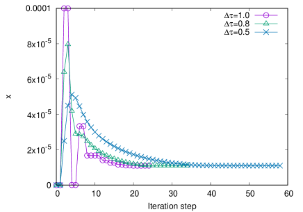
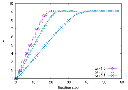
(a)	(b)
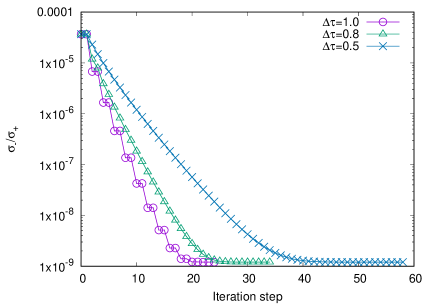
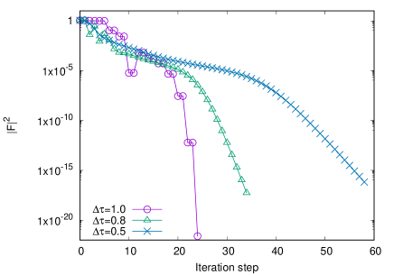
(c)	(d)

Figure 1: The numerical results obtained with the W4SV method for Powell’s badly scaled problem: (a) $x$, (b) $y$, (c) the ratio of the smaller to larger singular values $\sigma_{-}/\sigma_{+}$, (d) the error norm $|F|^{2}=f_{x}^{2}+f_{y}^{2}$. The different colors specify the values of $\Delta\tau$.

The singularity in the initial condition cannot be treated with the existing methods that need to invert the Jacobian matrix. We show in the following subsections how such singularities are handled with the W4SV method. The first example is the well-known Powell’s Badly Scaled function (32). If we choose the initial condition as $\bm{x}=(0,1)^{T}$, then even the NR method obtains the solution rather easily. We are faced with a difficulty, however, when we start the NR iteration from $\bm{x}=(1,1)^{T}$ as in Table 1. In fact, the Jacobian matrix associated with this problem is given at $\bar{x}=(x,y)^{T}$ as

$$J=\begin{pmatrix}10^{4}y&10^{4}x\\ -e^{-x}&-e^{-y}\end{pmatrix}.$$ (27)

Obviously, it is singular when $x=y$. In the existing root-finding methods using the inversion of Jacobian, one has to change the initial condition. As we show shortly, our W4SV method can solve the problem even from this initial condition.

Fig. 1 shows the evolutions in the W4SV method of (a) $x$, (b) $y$, (c) $\sigma_{-}/\sigma_{+}$ the ratio of singular values and (d) $|F|^{2}=f_{x}^{2}+f_{y}^{2}$ the norm of error for Powell’s badly scaled function. The initial condition is $\bm{x}=(0,1)^{T}$, which is non-singular. The different colors in the figure correspond to the choice from $\Delta\tau=1,0.8,0.5$. It is found from panels (a) and (b) of Fig. 1 that $x$ and $y$ are settled down to the solution for all the values of $\Delta\tau$. As shown in panel (c), the smaller singular value $\sigma_{-}$ approaches a small value as the iteration is closing to an end, while the iteration map is well-defined there. As expected from the analysis of the W4SV map near the solution in Lemma 3, the error decreases monotonically in Fig. 1 after the numerical solution $\bar{x}$ comes close to the solution.

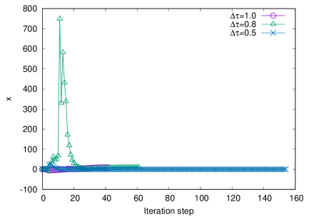
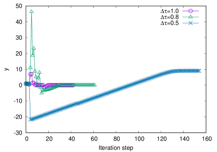
(a)	(b)
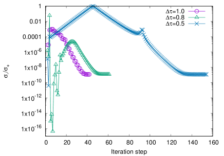
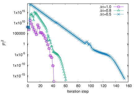
(c)	(d)

Figure 2: Same as Fig. 1 except for the initial condition $(1,1)^{T}$.

In Fig. 2, we display the same quantities as in Fig. 1 except for the initial guess, which is now set to $(1,1)^{T}$. This initial condition is singular and the application of the existing methods with the Jacobian inversion is simply impossible. Remarkably, the W4SV method successfully found the solution also in this case for all three values of $\Delta\tau$. As expected, the error decreases monotonically towards the end of iterations, as seen in (d) of Fig. 2. More importantly, the initial condition is singular  (see panel (c)) and is much farther away from the solution  (panel (d)) compared with the above case. Note that again for all three values of $\Delta\tau$ the W4SV method defines non-singular iteration map and successfully escapes from the initial singularity. It is observed, however, that the iteration maps kick the intermediate solutions in early iteration steps away from the solution. This happens because the intermediate solutions stay near the initial singilarity after a few iterations and the big factor $1/\sigma_{-}$ combined with large values of $|F|$ in the iteration map finally pushes the following solution away from the true solution. Nevertheless, once escaped from the vicinity of the initial singularity, the subsequent solutions start to move in the right direction and eventually converge to the solution. Note also that this system (32) is symmetric with respect to $x$ and $y$ and then there is another solution by exchanging $y$ for $x$ and $x$ for $y$ as results with $\Delta\tau=0.8$ and $\Delta\tau=1.0$ in Fig. 2.

3.2 Beale’s function

Beale’s function is given in Eq. (34) and the associated Jacobian matrix is

$$J=\begin{pmatrix}y-1&x\\ y^{2}-1&2xy\end{pmatrix}.$$ (28)

Since $\det J=x(y-1)^{2}$, the Jacobian matrix is singular at $x=0$ or $y=1$, corresponding to the column, respectively. If such a singular state is encountered during the iteration, the existing methods that utilizes the inverse of $J$ will be stuck there. As demonstrated in Fig. 3, which shows the same quantities as Fig. 1 obtained with the W4SV method with $\Delta\tau=0.5$ for this problem, our new method is able to reach the right answer without taking any special measure. We choose two singular states as the initial condition: $(1,1)^{T}$ and $(0,2)^{T}$, the results of which are displayed with circles and pluses, respectively.

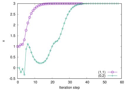
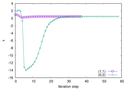
(a)	(b)
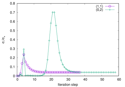
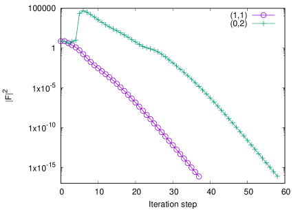
(c)	(d)

Figure 3: Same as Figs. 1 and 2 but for Beale’s problem (34). We choose $\Delta\tau=0.5$ for this problem. Circles and pluses denote the results for the different initial conditions: $(x,y)^{T}=(1,1)^{T}$ and $(x,y)^{T}=(0,2)^{T}$, respectively.

3.3 Fujisawa’s function

In order to further check the capability of singular avoidance by the W4SV method, we apply it to another numerically tough problem in Eq. (36), which we considered in our previous paper [7]. The Jacobian matrix is expressed as

$$J=\begin{pmatrix}2x&2y\\ 2xy&x^{2}\end{pmatrix},$$ (29)

the determinant of which is $\det J=2x(x^{2}-2y^{2})$. The initial condition with either $x=0$ or $x=\pm\sqrt{2}y$ is hence singular. Even if the initial condition is nonsingular, we know that this problem is difficult to solve numerically from initial conditions given below the lines $x=\pm\sqrt{2}y$, because it is likely that one of these singular points is encountered at some intermediate step during the iteration [7]. In Fig. 4, we show the results obtained with the W4SV method with $\Delta\tau=0.5$. The initial condition is either $(0,1)^{T}$, or $(0,-1)^{T}$. It is obvious that small singular values, that are encountered from time to time during the iterations, affect the intermediate solution at the next iteration step particularly when they are still far from the true solution as seen, for example, at around the $30\mathrm{th}$ iteration step in Fig. 4. It is also found, however, the W4SV method can avoid such situations and reach the right solution eventually. As in the previous case, the error decreases monotonically in the vicinity of the solution.

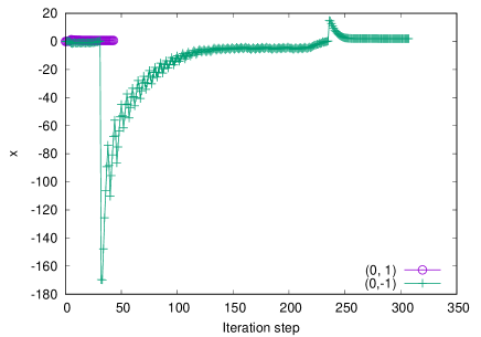
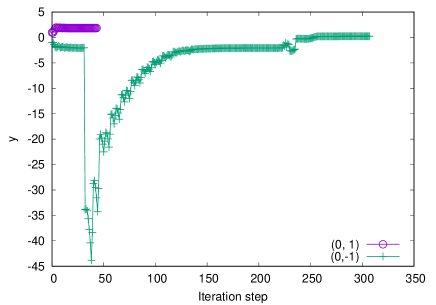
(a)	(b)
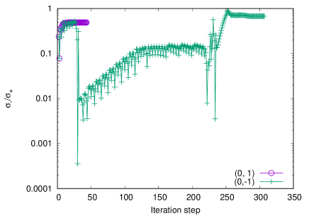
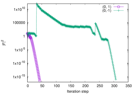
(c)	(d)

Figure 4: Same as Figs. 1-3 but for Fujisawa’s function. We set $\Delta\tau=0.5$ for this test. The initial condition is either  $(0,1)^{T}$ or $(0,-1)^{T}$.

4 Conclusion

In this article, we have proposed a new scheme to solve a set of nonlinear equations. It is an extension of the W4 method, a root-finder of our own devising that shows a nice global convergence and obtain solutions to various problems, for which existing methods such as the Newton-Raphson method failed [7]. The original W4 method has been successfully applied to different physics problems so far [8, 9, 10]. The extension reported in this article is meant to deal with the singular Jacobian, which we frequently encounter in practical applications and even the original W4 method finds difficulties in treating. This problem is actually common to all the existing root-finders that require the inversion of Jacobian. In the W4SV method, however, the iteration map is always well-defined and can reach the solution even for problems, for which the Jacobian is singular at the initial or intermediate step of iterations or at the true solution unless the very special condition (26) is satisfied. The results of the numerical tests in Sec. 3 for the well-known problems, albeit in two dimensions, strongly support the excellent capability of our new scheme.

In principle, our new scheme should be applicable to larger-dimensional problems, which often appear in computational science, physics and engineering. For efficient applications to those problems, however, it is necessary to (i) treat non-singular but ill-conditioned Jacobians more efficiently and (ii) reduce the computational cost in calculating singular vectors and singular values, which is the most cost-consuming part when the number of variables becomes larger. We will address these issues in the near future.

Appendix A Test problems

In the literature, there are many test problems for root-finders of nonlinear equation systems. We summarize here the two dimensional test problems. The problems to solve are written in general as $\bm{F}(x,y)=\left(f_{x}(x,y),f_{y}(x,y)\right)^{T}=\bm{0}$ together with the initial condition $\bar{x}_{0}$ for the iteration.

1. Rosenbrock’s problem:

   $$f_{x}(x,y) = 10(y-x^{2}),$$

   $$f_{y}(x,y) = 1-x,$$

   $$\bm{x}_{0} = (1.2,1)^{T}.$$ (30)

2. Freudenstein and Roth’s problem:

   $$f_{x}(x,y) = -13+x+\left((5-y)y-2\right)y,$$

   $$f_{y}(x,y) = -29+x+\left((y+1)y-14\right)y,$$

   $$\bm{x}_{0} = (6,3)^{T}.$$ (31)

3. Powell’s badly scaled problem:

   $$f_{x}(x,y) = 10^{4}xy-1,$$

   $$f_{y}(x,y) = e^{-x}+e^{-y}-1.0001,$$

   $$\bm{x}_{0} = (0,1)^{T}\ \mathrm{or}\ \bm{x}_{0}=(1,1)^{T}.$$ (32)

4. Brown’s badly scaled problem:

   $$f_{x}(x,y) = xy^{2}-2y+x-10^{6},$$

   $$f_{y}(x,y) = x^{2}y-2x+y-2\times 10^{-6},$$

   $$\bm{x}_{0} = (1,1)^{T}.$$ (33)

5. Beale’s problem:

   $$f_{x}(x,y) = 1.5-x(1-y),$$

   $$f_{y}(x,y) = 2.25-x(1-y^{2}),$$

   $$\bm{x}_{0} = (1,1)^{T}\ \mathrm{or}\ \bm{x}_{0}=(0,2)^{T}.$$ (34)

6. Hueso & Monteiro’s problem:

   $$f_{x}(x,y) = (x-1)^{2}(x-y),$$

   $$f_{y}(x,y) = (y-2)^{5}\cos(2x/y),$$

   $$\bm{x}_{0} = (1.5,2.5)^{T}.$$ (35)

7. Fujisawa’s problem:

   $$f_{x}(x,y) = x^{2}+y^{2}-4,$$

   $$f_{y}(x,y) = x^{2}y-1,$$

   $$\bm{x}_{0} = (0,1)^{T}\ \mathrm{or}\ \bm{x}_{0}=(0,-1)^{T}.$$ (36)

References

- [1] J. M. Ortega, W. C. Rheinboldt, Iterative solution of nonlinear equations in several variables, Vol. 30, Siam, 1970.
- [2] C. T. Kelley, Solving nonlinear equations with Newton method, Vol. 1, Siam, 2003.
- [3] A. S. Householder, The numerical treatment of a single nonlinear equation.
- [4] H. Ramos, J. Vigo-Aguiar, The application of newton method in vector form for solving nonlinear scalar equations where the classical newton method fails, Journal of Computational and Applied Mathematics 275 (2015) 228–237.
- [5] H. Ramos, M. T. T. Monteiro, A new approach based on the newton method to solve systems of nonlinear equations, Journal of Computational and Applied Mathematics 318 (2017) 3–13.
- [6] C. G. Broyden, A class of methods for solving nonlinear simultaneous equations, Mathematics of computation 19 (92) (1965) 577–593.
- [7] H. Okawa, K. Fujisawa, Y. Yamamoto, R. Hirai, N. Yasutake, H. Nagakura, S. Yamada, The W4 method: a new multi-dimensional root-finding scheme for nonlinear systems of equationsarXiv:1809.04495.
- [8] K. Fujisawa, H. Okawa, Y. Yamamoto, S. Yamada, Effects of rotation and magnetic field on the revival of a stalled shock in supernova explosions, Astrophys. J. 872 (2) (2019) 155. arXiv:1809.04358, doi:10.3847/1538-4357/aaffdd.
- [9] H. Suzuki, P. Gupta, H. Okawa, K.-i. Maeda, Post-Newtonian Kozai-Lidov Mechanism and its Effect on Cumulative Shift of Periastron Time of Binary PulsararXiv:2006.11545.
- [10] R. Hirai, T. Sato, P. Podsiadlowski, A. Vigna-Gomez, I. Mandel, Formation pathway for lonely stripped-envelope supernova progenitors: implications for Cassiopeia AarXiv:2008.05076.
- [11] J. Kou, Y. Li, X. Wang, Efficient continuation newton-like method for solving systems of non-linear equations, Applied mathematics and computation 174 (2) (2006) 846–853.
- [12] X. Wu, Note on the improvement of newton method for system of nonlinear equations, Applied Mathematics and Computation 189 (2) (2007) 1476–1479.
- [13] J. L. Hueso, E. Martínez, J. R. Torregrosa, Modified newton method for systems of nonlinear equations with singular jacobian, Journal of Computational and Applied Mathematics 224 (1) (2009) 77–83.
- [14] X. Fang, Q. Ni, M. Zeng, A modified quasi-newton method for nonlinear equations, Journal of Computational and Applied Mathematics 328 (2018) 44–58.
- [15] J. J. Moré, B. S. Garbow, K. E. Hillstrom, Testing unconstrained optimization software, ACM Transactions on Mathematical Software (TOMS) 7 (1) (1981) 17–41.
-
[16]
H. Okawa,
Demonstration
of the W4SV method in Python (2022).
URL {https://hir0ok.github.io/w4/w4demo_W4SV_TestFunctions.html}