Multicomponent imaging of the Fermi gamma-ray sky
in the spatio-spectral domain

The gamma-ray sky as seen by the Large Area Telescope (LAT) on board the Fermi satellite is a superposition of emissions from many processes. To study them, a rich toolkit of analysis methods for gamma-ray observations has been developed, most of which rely on emission templates to model foreground emissions. Here, we aim to complement these methods by presenting a template-free spatio-spectral imaging approach for the gamma-ray sky, based on a phenomenological modeling of its emission components. It is formulated in a Bayesian variational inference framework and allows a simultaneous reconstruction and decomposition of the sky into multiple emission components, enabled by a self-consistent inference of their spatial and spectral correlation structures. Additionally, we formulated the extension of our imaging approach to template-informed imaging, which includes adding emission templates to our component models while retaining the “data-drivenness” of the reconstruction. We demonstrate the performance of the presented approach on the ten-year Fermi LAT data set. With both template-free and template-informed imaging, we achieve a high quality of fit and show a good agreement of our diffuse emission reconstructions with the current diffuse emission model published by the Fermi Collaboration. We quantitatively analyze the obtained data-driven reconstructions and critically evaluate the performance of our models, highlighting strengths, weaknesses, and potential improvements. All reconstructions have been released as data products.

1 Introduction

Situated at the upper end of the electromagnetic spectrum, gamma rays bear witness to highly energetic processes. Because of their low interaction cross-section with most matter and radiation, gamma rays in the GeV to TeV range provide a window into their generation sites, which in other parts of the electromagnetic spectrum is often obscured by matter in the line of sight.

Based on observations of the gamma radiation, the processes and objects involved in creating it can be studied. This includes the production, acceleration, and dissemination of cosmic rays (CRs; Grenier et al. 2015; Tibaldo et al. 2021; Liu et al. 2022), whose interaction with matter and radiation fields contribute the majority of observed gamma rays and potentially dark matter (DM), whose properties can be constrained based on searches of dark matter annihilation (DMA) emission (Bergström 2000; Gianfranco et al. 2005).

The gamma-ray fluxes that reach Earth are a superposition of emissions from various sources: First, a strong Galactic foreground is produced by interactions of CRs with the interstellar medium (ISM) of the Milky Way. The dominant processes for this are inelastic collisions of CR protons with protons present in the thermal ISM, which create neutral pions that quickly decay into gamma rays, bremsstrahlung produced by cosmic ray electrons (CRe-) and positrons (CRe+) in ionized gas, and inverse Compton (IC) up-scattering of photons from the interstellar radiation field (star light, thermal infrared, and microwave emission from dust grains) and the cosmic microwave background by CRe- and CRe+. These Galactic emissions trace the distribution of the respective target and CR populations within the Galaxy, making them span large parts of the sky and giving them characteristic spatial structures.

Second, there is a large population of very localized gamma-ray emitters, appearing as point sources (PSs) from Earth, including blazars, pulsars, and supernova remnants (Abdo et al. 2010; Nolan et al. 2012; Acero et al. 2015; Abdollahi et al. 2020, 2022b). Because these objects actively accelerate CRs, their gamma-ray spectra differ somewhat from the spectra observed for the Galactic ISM emission. Some of them, because of their relatively close proximity to Earth, appear as extended objects in the sky (Lande et al. 2012; Ackermann et al. 2017b, 2018a). Notable examples include the Vela, Crab, and Geminga pulsar wind nebulae.

Third, there is an isotropic background of gamma radiation from faint Galactic and extragalactic sources (see Fornasa & Sanchez-Conde 2015, Ackermann et al. 2018b, and Roth et al. 2021). To contrast the first and third group from PSs, the former are usually referred to as diffuse emissions.

Today’s largest data set of gamma-ray observations is based on measurements by the Fermi Large Area Telescope (LAT; Atwood et al. 2009). The LAT is an orbital pair-conversion telescope, sensitive in the MeV to TeV energy range, that features a large instantaneous field of view (roughly 20 % of the sky) and an angular resolution from about 3 degrees at 0.1 GeV to a few arcminutes at TeV energies. It detects individual gamma-ray photons and records an estimate of their origin direction, energy, and arrival time.

Notably, Fermi LAT observations led to the discovery of the so-called Fermi bubbles (FBs; Su et al. 2010; Ackermann et al. 2014), two symmetric large-scale emission structures located north and south of the Galactic center (GC), and the Galactic center excess (GCE; Goodenough & Hooper 2009; Hooper & Goodenough 2011), a population of gamma rays originating from within a few degrees around the GC that are not predicted by emission models based on observations in other energy bands. The discovery of the GCE sparked a still ongoing debate about its origin, with the leading hypotheses being DMA emissions (Hooper & Goodenough 2011) and a dense population of faint millisecond pulsars (Abazajian 2011). Together with the study of the extragalactic gamma-ray background, the debate about the GCE origin led to the development of a broad range of analysis methods for gamma-ray data sets, all addressing the fundamental difficulty of attributing gamma-ray fluxes to specific production processes.

Here, we present an overview of established gamma-ray analysis approaches to provide context for the method we introduce. A fundamental technique employed in almost all analyses is emission template fitting. For this, the spatial and/or spectral distribution of gamma-ray emission from different channels is predicted based on other astrophysical observations, theoretical considerations, or, in the case of only gamma-visible structures, preprocessed gamma-ray data. The obtained templates are then used in parametric models of the gamma-ray sky, which are fit to the observed data. This way, even complex skies can be adequately expressed with only a few fit parameters if correct templates of all contained emission components are available. The emission from major channels can be predicted to a high degree of accuracy (see Ackermann et al. 2012, Acero et al. 2016, Buschmann et al. 2020, and Karwin et al. 2023 for details of the template creation). Because of this success in modeling, most analyses make use of templates to account for the emission from these channels.

In the study of extended and diffuse emissions, a second fundamental technique (often combined with template fitting, but also used in other ways) is the masking of known PSs. For this, data bins within a chosen distance to known PSs are discarded. This alleviates the need to model bright PS emissions and reduces the sensitivity of the analysis to instrumental point spread mismodeling. When using PS masking, a trade-off between PS flux contamination and data set size degradation needs to be made.

As laid out by Storm et al. (2017), likelihood-based gamma-ray analyses can be understood on a continuum from low to high parameter count, representing different trade-offs between parameter space explorability, statistical power, goodness of fit, and sensitivity to unexpected emission components. On the low parameter count end of the continuum are pure template fitting analyses, with only a few parameters per emission template (global or large-area scaling constants). Many early publications of the Fermi Collaboration are based on this approach (see for example Abdo et al. 2010, Abdo et al. 2010, Ackermann et al. 2012, and Ackermann et al. 2012).

As emission structures not predicted by other observations were found, such as the FBs, multiple methods for deriving data-driven templates for these structures were developed. Examples include the work of Casandjian (2015), which models emission from IC interactions of CRe- and CRe+ with the cosmic microwave background via pixel-wise fits of an IC emission spectrum model to filtered and point spread function (PSF) de-convolved residuals of the already templated foregrounds, and post-processed using a spatial domain 2° wavelet high-pass filter. Similarly, Acero et al. (2016) built models of “extended excess emissions” that include the FBs and Loop 1 from wavelet-filtered baseline model residuals. Based on the combination of conventional and data-driven templates, the diffuse gamma-ray sky can be modeled to a high fidelity (see for example Calore et al. 2022).

Many publications assume the remaining misfits to point out the existence of true excess populations. These are typically studied by extending the template model with additional parametric models of the excesses, derived from the properties of the hypothesized excess origins. The comparative quality of fit using different excess models is then taken as evidence in favor of or against the respective origin hypotheses. Many analyses of the GCE are based on this approach.

A notable family of techniques that follow this pattern are photon count statistics methods, first introduced for gamma rays by Malyshev & Hogg (2011). They exploit the difference in photon statistics expected from truly diffuse emitters and dense but faint PS populations to infer properties of sub-detection-threshold PSs, for example their source count distribution (SCD). Lee et al. (2016) and Mishra-Sharma et al. (2017) implemented this concept under the name non-Poissonian template fitting (NPTF). Independently, Zechlin et al. (2016) formulated methods based on photon count statistics centered around one-point probability distribution functions (1pPDFs), which include pixel-dependent variations in the expected photon statistics, for example from the instrument response. The authors used this to study GCE signals, DM signals, and the extragalactic isotropic background (Zechlin et al. 2018). Analysis approaches of the photon count statistics family have been extended to other modalities, including neutrino astronomy (Feyereisen et al. 2018; Aartsen et al. 2020).

A conceptual extension of 1pPDF methods to methods based on two-point correlation statistics was shown by Manconi et al. (2020). They derived expected angular power spectrum (APS) models for different emission types, similar to the 1pPDF models. Using the 1pPDF and APS models, they studied the extragalactic background using Fermi LAT data and find good agreement between the two statistics. Baxter et al. (2022) show with synthetic data how approximate Bayesian computation (Sisson et al. 2007; Beaumont et al. 2009; Blum & François 2010), a likelihood-free method, could be applied to 1pPDF studies of the extragalactic gamma-ray emissions.

A crucial limitation of template-based approaches is their dependence on accurate emission templates. As has been pointed out on multiple occasions, a mismodeling of the foreground emissions can severely bias template-based analyses. An example of this is the disagreement between Leane & Slatyer (2020), who studied the ability of NPTF to recover an artificially injected DM signal and report NPTF to be biased toward neglecting it, and Buschmann et al. (2020), who argue the observed bias is caused by insufficiently accurate foreground emission models.

To eliminate templating errors post creation, approaches for optimizing existing templates in a data-driven way have been published. Buschmann et al. (2020) demonstrate a template optimization scheme in the spherical harmonic (SH) domain, adjusting the normalization constant of all SH components of the templates individually and reassembling updated versions of the templates from the scaled SH components afterward.

To mitigate biases introduced by template misfits, a move toward additional nuisance parameters that explicitly model the template misfits can be observed. This includes various imaging techniques that derive data-driven reconstructions of the whole sky, as well as works toward full modifiability of templates.

Criticizing poor qualities of fit in previous template analyses, Storm et al. (2017) introduced the SkyFACT framework. It enables the inclusion of full-resolution Gaussian template modification fields into sky reconstructions, making it a hybrid parameter estimation and imaging method. Spatio-spectral distributions of emission components are modeled by the outer product of spatial and spectral templates and (if desired) their respective modification fields. They introduced a custom regularization term for the modification fields that preserves the convexity of the optimization problem. By consecutively adding modification fields to a template analysis of the Fermi LAT data set, the authors demonstrate the effect of transitioning from low to high parameter count analyses. For the model parameter estimation, the authors employed a quasi-Newton method and estimated the errors of individual model parameters via the Fisher information matrix and a sparse Cholesky decomposition (see Storm et al. 2017 for details). This work can also be used to derive optimized emission templates as demonstrated by Calore et al. (2021), who obtained optimized emission templates with a SkyFACT fit of the LAT data and then performed a 1pPDF analysis of the residuals.

Mishra-Sharma & Cranmer (2020) introduced a variational inference framework that includes Gaussian process-based template modification fields and a neural network (NN) to predict posterior distributions of other model parameters depending on the modification field state. The Gaussian processes are implemented using a deep learning (DL) framework, making the implementation compatible with graphics processing units. The authors demonstrate the potential of their method by analyzing the GC emission as captured by the Fermi LAT.

Selig et al. (2015) demonstrate a template-free imaging of the gamma-ray sky based on the D³PO algorithm (Selig & Enßlin 2015). Here, the gamma-ray emissions are modeled freely, with prior statistics of the logarithmic diffuse sky brightness encoded in a Gaussian processes with a to-be-inferred statistically homogeneous correlation structure, and PS fluxes implemented via spatial sparsity enforcing priors. This work performed the reconstructions for each energy band independently, only making use of spatial correlations to guide the reconstruction. Pumpe et al. (2018) developed the D⁴PO algorithm to additionally exploit spectral correlations for spatio-spectral imaging.

A benefit of these high parameter count reconstruction methods is their potential to have a higher sensitivity to unexpected emission components, especially to small structures, as they do not impose as strong a priori assumptions about the distribution of gamma-ray flux as fixed template-based fits do. However, this comes at the price of a higher vulnerability to instrument mismodeling in data-driven analyses, where an accurate modeling of the instrument response is crucial, and potentially a higher susceptibility to measurement noise.

A different line of inquiry involves wavelet-based methods. Schmitt et al. (2012) demonstrate an iterative de-noising and PSF de-convolution algorithm based on SH wavelets with synthetic LAT data. Bartels et al. (2016) performed a template-free comparison of GCE excess models based on how well they predict wavelet coefficient statistics of Fermi data at length scales where no foreground structure is expected. Balaji et al. (2018) show a wavelet-based analysis of photon counts unexplained by state-of-the-art emission templates and derive data-driven maps of the emissions of the FBs, the GCE, and the “cocoons” inside the FBs.

Finally, over the last few years, a number of promising DL-based gamma-ray data analysis approaches have been developed, training NNs to directly predict quantities of interest from binned photon counts. The NNs are trained on synthetic data generated with existing emission templates and various mixtures of additional emission structures, tested on further synthetic data samples, and then applied to the Fermi LAT data.

Caron et al. (2018) demonstrate a convolutional NN trained to predict the PS emission fraction of the GCE directly from photon count data. List et al. (2020) demonstrate a graph convolutional NN trained to predict unmixed gamma-ray emission maps for the GC region, including a separation of smooth DM emissions and GCE PS emissions. They report emission component recovery accuracies to the percent level on a synthetic test data set and provide estimates of the aleatoric uncertainty for each component. List et al. (2021) extended this work, predicting the SCD of the identified GCE emissions in a nonparametric form. Recently, Mishra-Sharma & Cranmer (2022) published an orthogonal approach that uses NNs to enable fast simulation-based inference (SBI). They simultaneously trained a convolutional-NN-based feature extractor and a normalizing-flow-based inference network to predict posterior parameters of a generative (forward) gamma-ray sky model from photon count data. With this SBI pipeline, they were able produce posterior samples of the forward model parameters conditioned on the Fermi LAT data.

In this article we build on methods developed in the context of information field theory (IFT; Enßlin et al. 2009; Enßlin 2013, 2019) following Selig et al. (2015), Storm et al. (2017), Pumpe et al. (2018), and Mishra-Sharma & Cranmer (2020). We demonstrate a template-free spatio-spectral imaging approach for the gamma-ray sky using a diffuse emission model, published and validated in Arras et al. (2021) and Arras et al. (2022), and a PS emission model built following the same philosophy. We show how the approach can be extended into a hybrid approach of imaging and template analyses. For this, we include emission templates in our model but retain the data-drivenness of the template-free imaging. We call this hybrid approach “template-informed imaging.” We created two corresponding sky emission models (template-free and template-informed) and reconstructed the Fermi LAT ten-year gamma-ray sky based on them. To test the presented approaches, we analyzed the spatio-spectral sky reconstructions obtained with the two models in light of results from the literature. Finally, we briefly discuss how the presented approach can be extended by or merged with existing emission modeling approaches.

This paper is structured as follows: In Sect. 2 we describe the models and methods used, as well as our data selection. Section 3 showcases the results obtained with the presented imaging approach. Therein, Sects. 3.1 and 3.2 provide the sky maps obtained with the template-free and template-informed imaging, as well as analyses of their features. Section 3.3 then compares the two obtained sky maps. In Sect. 4 we discuss our findings, highlighting their strengths and limitations. We conclude in Sect. 5.

The appendices are structured as follows: Appendix A gives further details on the sky models. Appendix B describes how we implemented the instrument response model. Appendix C details how we created the spatio-spectral sky map renderings contained in this work. Finally, Appendix D contains supplementary figures.

2 Models and methods

2.1 General methods

In this paper we present a Bayesian imaging approach. Bayesian inference assigns probability values $\mathcal{P}(s|d)$ to every possible configuration of a quantity of interest (“signal”) $s$, given the data $d$. This assignment takes into account the likelihood $\mathcal{P}(d|s)$, the probability of having obtained the observed data, $d$, for a given $s$, and the prior $\mathcal{P}(s)$, the probability of $s$ given pre-measurement knowledge, via Bayes’ theorem:

$$\mathcal{P}(s|d)=\frac{\mathcal{P}(d|s)\,\mathcal{P}(s)}{\mathcal{P}(d)}.$$ (1)

The term $\mathcal{P}(d)=\int\mathrm{d}s\,\mathcal{P}(d|s)\,\mathcal{P}(s)$ (“evidence”) ensures proper normalization of the so-called posterior probability distribution $\mathcal{P}(s|d)$.

In our case, the signal of interest is the time-averaged gamma-ray photon flux density of the sky $\Phi(x,E)$ as a function of photon origin direction $x$ and energy $E$ in the energy interval of 0.56–316 GeV and the first 10 years of LAT operation. $\Phi(x,E)$ is a continuous, strictly positive function in both variables. We cannot numerically represent and reconstruct such general functions without approximation, so we derive a discretization-aware signal formulation related to $\Phi(x,E)$ in Sect. 2.2.

We performed a binned analysis, meaning that the data with respect to which we estimate the posterior signal distribution is a high-dimensional histogram of photons recorded by the LAT. The LAT instrument response depends on photon properties such as the photon energy, the incidence direction with respect to the instrument orientation $\psi=(\theta,\phi)$, and the location of the pair conversions within the instrument (FRONT or BACK conversions, Ackermann et al. 2012). To include this effect in our model of the measurement, the photon events were binned along the dimensions x, E, $\phi$, and event types, and we model the response function for each histogram bin individually. We assume the counts in the histogram to follow Poissonian statistics:

$$\mathcal{P}(d|\lambda)=\frac{\lambda^{d}}{d!}\,\mathrm{e}^{-\lambda},$$ (2)

with $\lambda$ being the histogram-bin photon rate predicted by the signal $\mathrm{s}$ and our instrument response model $\mathrm{R}$: $\lambda=\mathrm{R}(\mathrm{s})$. Section 2.4 provides details of the instrument response modeling and Sect. 2.5 details the event selection.

To make our template-free imaging robust against measurement noise, we need to constrain the signal model. In the Bayesian framework, constraints like this are naturally introduced via the signal prior, which is based on our physical understanding of the signal. In Sect. 2.3 we describe how we express our prior knowledge on the reformulated signal quantity. We implement the instrument, sky models and the reconstruction using the numerical information field theory (NIFTy) framework (Selig et al. 2013; Steininger et al. 2019; Arras et al. 2019), Version 8.4. The signal priors are expressed in the form of generative models, following Knollmüller & Enßlin (2018).

One significant challenge in performing inferences of high-dimensional parameter vectors, as is necessary for the given imaging problem, is the curse of dimensionality. With rising parameter number, exploring the full parameter space in the inference quickly becomes infeasible. In this work, we rely on metric Gaussian variational inference (MGVI; Knollmüller & Enßlin 2019), a variational inference framework built for the high parameter number limit. It allows us to iteratively optimize a set of posterior samples for models with millions of parameters, from which posterior estimates of quantities of interest can be derived and their variances can be inspected.

2.2 Discretized signal definition

In the process of binning the event data into count maps, information on the flux structure within the spatial and spectral bins is lost. As we want to make our analysis as data-driven as possible and correspondingly do not want to impose strong assumptions on the structure of $\Phi(x,E)$ within the bins, we do not try to reconstruct $\Phi(x,E)$, but instead infer its integrated counterpart,

$$I_{\mathrm{ij}}=\frac{1}{|\Omega_{\mathrm{j}}|}\int_{E_{\mathrm{i}}}^{E_{\mathrm{i+1}}}dE\int_{\Omega_{\mathrm{j}}}dx\;\Phi(x,E),$$ (3)

where $\Omega_{j}$ is the j-th sky pixels area (solid angle) and the energy bin boundaries are chosen equidistantly on a log-energy scale. Structural information on bin-sized scales and above is retained in the binned count maps, allowing us to do relatively unconstrained reconstructions of $I_{\mathrm{ij}}$. The next section outlines what this means in practice.

One side effect of the binning into logarithmically equidistant energy bins is a change in flux scaling with energy. For logarithmically equidistant energy bins, the bin width is proportional to the base energy of the bins. Because of this, $I_{\mathrm{ij}}$ effectively scales with energy like $E\cdot\Phi$ and spectral index estimates based on $I_{\mathrm{ij}}$ need to be adjusted by $1$ to compare with spectral index estimates for un-integrated fluxes, $\Phi$:

$$\alpha_{\,I}=\alpha_{\,\Phi}+1.$$ (4)

We pixelized the sky based on the HEALPix scheme introduced by Gorski et al. (2005) and use an $\mathtt{nside}$ value of 128, corresponding to a pixel size of approximately 0.46°. In the energy dimension, we pixelized the signal with a density of four bins per decade between 0.56 GeV and 316 GeV.

2.3 Formulation of prior knowledge and image regularization

2.3.1 General modeling of the sky brightness

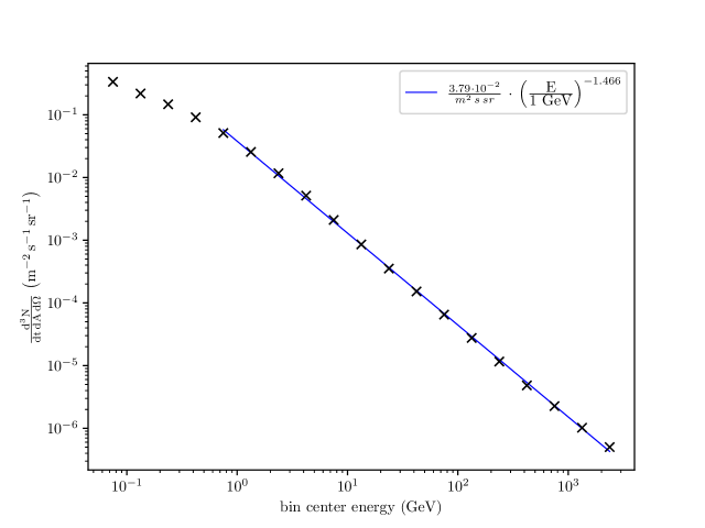
Figure 1: Sky-averaged estimate of $I_{\mathrm{ij}}$ on log-log scale based on the exposure- and effective-area-corrected photon count map. Because we show fluxes integrated over logarithmically equidistant energy bins, spectral index values are offset by $+1$ with respect to un-integrated energy spectra (see Eqs. 3 and 4 for details).

Both $\Phi(x,E)$ and $I_{\mathrm{ij}}$ are strictly positive and vary over many orders of magnitude. A rudimentary estimate of $I_{\mathrm{ij}}$ can be obtained by dividing the data histogram by the exposure time and instrumental sensitivity for each data bin. Figure 1 shows this quantity averaged over the spatial (x) and incidence direction ($\theta$) domains. We observe it to follow a power law with a spectral index of $-1.466$ in the 0.56–316 GeV energy range studied in this paper. We note that this is the spectral index per logarithmic energy. The corresponding spectral index per energy is $-2.466$.

Motivated by this, we model the bin-integrated sky flux as

$$I_{\mathrm{ij}}=I_{0}\cdot\left(\frac{E_{i}}{E_{0}}\right)^{\alpha}\cdot{10}^{\,\tau_{\mathrm{ij}}},$$ (5)

with

$$\tau_{\mathrm{ij}}=\log_{10}\left(\frac{I_{\mathrm{ij}}}{I_{\mathrm{0}}\cdot(E_{\mathrm{i}}/E_{\mathrm{0}})^{\alpha}}\right)$$ (6)

giving the variations in the sky with respect to a power-law spectrum with spectral index $\alpha$ on a decadic logarithmic scale. The employed value of the reference flux scale $I_{\mathrm{0}}$ and the reference energy $E_{\mathrm{0}}$ are provided in the following section.

This parameterization is convenient as it allows us to jointly model the spatial variations in the integrated sky flux and its spectral deviations from power-law spectra, both of which are expected to take values over many orders of magnitude, on linear scales. The modeling via logarithmic flux variations allows us to accommodate this.

The sky exhibits correlations of the logarithmic fluxes over the spatial and spectral domains, respectively, $\langle\tau_{\mathrm{ij}}\,\tau_{\mathrm{i^{\prime}j^{\prime}}}\rangle_{(\tau)}$, with $\langle f(\tau)\rangle_{(\tau)}:=\int\mathrm{d}\tau\,\mathcal{P}(\tau)\,f(\tau)$ being the expectation value of some function $f$ over the probability distribution on $\tau$ as indicated by the index. In the spectral direction the correlation structures emerge from high-energy astroparticle processes, while the spatial correlations are related to macroscopic events, for example the temporal evolution of our Galaxy. We therefore assume these correlations to be separable in the spatial and energy direction. A priori, we also do not want to single out any directions or energy scale, so we additionally assume statistical homogeneity with respect to locations and log-energies $y_{\mathrm{i}}=\log_{10}\left(E_{\mathrm{i}}/E_{\mathrm{0}}\right)$, $\langle\tau_{\mathrm{ij}}\,\tau_{\mathrm{i^{\prime}j^{\prime}}}\rangle_{(\tau)}=C(|x_{\mathrm{j}}-x_{\mathrm{j^{\prime}}}|)\,D(|y_{\mathrm{i}}-y_{\mathrm{j^{\prime}}}|)$, where we changed from the energy $E$ to the log-energy coordinate $y$. By using the log-energy coordinate $y$ and the assumption of homogeneous spectral correlations, we assume that the to be reconstructed energy spectra behave similarly over several decades in energy.

Spatial homogeneity of the correlations of $\tau$ expresses the assumption that the relative contrast of emission is structured similarly everywhere on the sky. This is not true in general, as for example point-like sources and diffuse emission certainly differ morphologically. Similarly, hadronic and leptonic emission should exhibit different structures due to the differently structured target densities, those of the nuclei and photons, respectively. Consequently, we model the total gamma-ray flux as a superposition of several emission processes $I_{\mathrm{ij}}^{\mathrm{\>comp}}$ (in the following “components”), always including point-like emission and one or more diffuse emission components. Each follows the functional form outlined in Eq. 5 and has its own correlation structure:

$$\langle\tau_{\mathrm{ij}}^{\mathrm{\>c}}\tau_{\mathrm{i^{\prime}j^{\prime}}}^{\mathrm{\>c^{\prime}}}\rangle_{(\tau)}=\delta_{\mathrm{c,\,c^{\prime}}}\,C^{\mathrm{\>c}}(|x_{\mathrm{j}}-x_{\mathrm{j^{\prime}}}|)\,D^{\mathrm{\>c}}(|y_{\mathrm{i}}-y_{\mathrm{i^{\prime}}}|).$$ (7)

A priori, we assumed each component to be uncorrelated with the others. Here $C^{\mathrm{\>c}}(\Delta x)$ is the spatial correlation function of component c and $D^{\mathrm{\>c}}(\Delta y)$ the spectral one. The Kronecker-delta $\delta_{\mathrm{c,\,c^{\prime}}}$ encodes a priori independence between the different components. This separability of the spatial and spectral correlations expresses the assumption that at different spatial locations of an emission component one expects similar, but not identical, spectral structures and vice versa.

The corresponding models of $\tau^{\mathrm{\>c}}$ were built based on the Gaussian correlated field model introduced by Arras et al. (2021, Sect. 3.4) and Arras et al. (2022). It allows us to translate prior knowledge on the correlation functions $C^{\mathrm{\>c}}$ and $D^{\mathrm{\>c}}$ into hierarchical generative models of $\tau^{\mathrm{\>c}}$. During reconstruction, a self-consistent pair of correlation functions and $\tau$s was inferred, providing a data-informed regularization of the inferred component sky maps without a priori imposing specific spatio-spectral flux shapes or flux intensity scales. Appendix A provides details of the generative modeling.

Flux from point-like sources can be modeled in this way as well. Assuming their location and brightness to be independent, their spatial correlation function is a delta function, $C^{\mathrm{\>point}}(\Delta x)=\delta(\Delta x)$. Each sky pixel harbors the photon flux contributed by all PSs situated within it. Since the set of PSs comprises a large variety of different physical objects, the energy spectra and total brightness values found for the pixels are expected to strongly differ across the sky. To accommodate this, we model the PS energy spectra differently from the diffuse energy spectra. Similarly to the diffuse energy spectra, we model them as following power-law spectra with variations on logarithmic scales. However, each pixel has an individual power-law spectral index $\alpha^{\mathrm{\>point}}_{\mathrm{\;j}}$ and the logarithmic deviations from pure power-law spectra are modeled for each pixel separately with a Gaussian process along the spectral dimension $\epsilon_{\mathrm{ij}}$, which we parameterized such that it naturally models sharp spectral features in the PS energy spectra.

Furthermore, the total brightness distribution function of the PS pixels $\mathcal{P}(I^{\mathrm{\>point}}_{\mathrm{tot,\,j}})$ is modeled as following a power-law distribution in pixel brightness $I^{\mathrm{\>point}}_{\mathrm{tot,\,j}}$ with a fixed power-law index of $-2.5$ and an exponential cutoff at low brightness values for normalizability. This corresponds to the assumption of a uniform source distribution in a steady-state and statically homogeneous Euclidean universe (Ryle 1950; Mills 1952). This is a simplifying assumption and will bias the found source distribution, but was chosen for simplicity.

The PS component is thus modeled as

$$I^{\mathrm{\>point}}_{\mathrm{ij}}=I^{\mathrm{\>point}}_{\mathrm{tot,\>j}}\cdot\frac{f_{\mathrm{spec,\>ij}}}{\sum_{\mathrm{i}}f_{\mathrm{spec,\>ij}}};\;\;f_{\mathrm{spec,\>ij}}={10}^{\>\alpha_{\mathrm{j}}\cdot y_{\mathrm{i}}\,+\,\epsilon_{\mathrm{ij}}}.$$ (8)

We chose the prior brightness mean to be two orders of magnitude below the expected diffuse emission brightness mean, to avoid introducing an isotropic background via the PS component. This effectively makes the PS brightness prior sparsity-enforcing, as PSs need to deviate by many standard deviations from the prior mean to contribute significant amounts of flux. This removes the degeneracy between the diffuse and PS components, which in principle could both account for the full sky flux (as we have a PS in every pixel). By biasing the PSs toward insignificant contributions we can ensure PS flux is only reconstructed when strongly suggested by the data. Section 4 provides a discussion of potential effects of our choices regarding the PS component prior.

To summarize, we assume the log-flux correlation function of the components to be separable in spatial and log-energy direction. This does not imply the sky components themselves to be separable into spatial and spectral component functions, but favors such a separability unless the data requests nonseparable spatio-spectral structures. This is suboptimal for distinct extended objects (Lande et al. 2012; Ackermann et al. 2017b, 2018a) that are neither well represented by the PS emission field nor correctly characterized by the spectra and spatial properties of any of the all-sky diffuse emission fields. Image reconstruction artifacts and misclassifications with respect to the assumed sky component classes are expected to happen for such objects in the current approach. Still, the majority of gamma-ray emission in the studied energy interval is expected to fit these models and is efficiently parameterized by them, as the reconstruction results show. The following subsection defines a template-free gamma-ray sky model, M1, based on the given concepts.

2.3.2 Template-free imaging model, M1

Model M1 for the template-free reconstruction consists of a single diffuse emission component $I^{\mathrm{\>diff}}$ and a PS component $I^{\mathrm{\>point}}$ as described in the previous section. Appendix A provides details of the M1 sky model, including a table of prior parameter values used. Here, we want to highlight a few especially important model parameters that most strongly determine the characteristics of the modeled components.

First, both the PS and diffuse models contain power laws along the energy dimension, for which a priori spectral indices need to be defined. Because we model flux integrated over logarithmically equidistant energy bins $I_{\mathrm{ij}}$, but in literature spectral indices are usually defined for un-integrated fluxes $\Phi$, we adjusted spectral index values obtained from literature according to Eq. 4. In case of the diffuse component $I^{\mathrm{\>diff}}$, we set the adjusted a priori spectral index to $\alpha^{\mathrm{\>diff}}=-1.466$, the value obtained from the estimate of $I_{\mathrm{ij}}$ based on the exposure- and effective-area-corrected data (see Fig. 1). Here we used the assumption that the gamma-ray sky is dominated by diffuse emission, such that we can take the average spectral index observed for the estimate of $I_{\mathrm{ij}}$ as the prior mean for the diffuse component spectral index without modification.

For the PS component, the spectral index prior $\mathcal{P}(\alpha^{\mathrm{\>point}}_{\mathrm{j}})$ was set according to Abdollahi et al. (2020, Fig. 16), from which we estimated a mean PS spectral index of $\alpha_{\Phi}=-2.25$ and a spectral index standard deviation of $0.30$. Adjusting for the fact that we model flux integrated over logarithmic energy bins, we set the adjusted a priori mean spectral index of the PS pixels to $\mu_{\mathrm{ap}}:=\langle\alpha^{\mathrm{\>point}}_{\mathrm{j}}\rangle_{\mathrm{prior}}=-1.25$ and the prior spectral standard deviation to $\sigma_{\mathrm{ap}}=0.30$ (unchanged).

Secondly, we needed to specify how much the overall brightness of the diffuse component can vary with respect to the reference scale $I^{\mathrm{\>diff}}_{\mathrm{0}}$. This model property is controlled by the prior on the mean of $\tau^{\mathrm{\>diff}}$, for which we chose a zero-centered Gaussian distribution with a standard deviation of $0.5$. This corresponds to a log10-normal prior on the best-fit diffuse brightness scale $I^{\mathrm{\>diff}}_{\mathrm{0,\,bf}}$, and allows our reconstruction to globally scale up or down the diffuse flux by a factor of 3 within one prior standard deviation and a factor of 10 with two prior standard deviations. This gives the reconstruction considerable freedom to correct a suboptimally chosen reference brightness scale $I^{\mathrm{\>diff}}_{\mathrm{0}}$.

Third, we needed to specify by how many orders of magnitude $\tau^{\mathrm{\>diff}}$ should be able to locally modify the flux density of $I^{\mathrm{\>diff}}$. This property of the model is controlled by the prior standard deviation of the fluctuations in $\tau^{\mathrm{\>diff}}$ with respect to its mean. We chose a prior mean of $0.75$ for this parameter, meaning the reconstruction can locally change the $I^{\mathrm{\>diff}}$ flux density by $0.75$ orders of magnitude within one prior standard deviation and by $1.5$ orders of magnitude within two prior standard deviations. Put another way, this assumes the spatial fluctuations of $I^{\mathrm{\>diff}}$ lie on the order of three orders of magnitude.

Lastly, the correlated field model employed for $\tau^{\mathrm{\>diff}}$ contains priors for the spatial and spectral correlation structure of the fluctuation field $\tau^{\mathrm{\>diff}}$. This serves to encode our prior knowledge on the spatial and spectral correlation structure of $\tau^{\mathrm{\>diff}}$ and $I^{\mathrm{\>diff}}$. Appendix A provides a more mathematical explanation of this model component, but for the sake of completeness, we give a short summary here. The spatial correlation structure model in $\tau^{\mathrm{\>diff}}$ assumes a priori that the spatial power spectrum follows a power law in angular harmonic mode scale $C_{\mathrm{\ell}}\propto\ell^{\>\beta}$. For the prior distribution of the power-law index, $\beta$, we chose a Gaussian distribution $\mathcal{N}\left(\beta\>|-3,\,0.25\right)$. This corresponds to assuming that the spatial structure of $I^{\mathrm{\>diff}}$, which needs to take up small-scale hydrogen density correlated features and larger scale smooth emission structures alike, is smoother than integrated Brownian noise (Wiener process). The energy dimension correlation structure model in $\tau^{\mathrm{\>diff}}$ assumes a priori that the spectral dimension power spectrum follows a power law in harmonic energy mode scale $D_{\mathrm{q}}\propto\mathrm{q}^{\>\gamma}$. For the prior distribution of the power-law index, $\gamma$, we chose a Gaussian distribution $\mathcal{N}\left(\gamma\>|-3.5,\,0.25\right)$. This corresponds to a priori smoother structures in the energy spectrum dimension than in the spatial domain, as is expected for most gamma-ray production processes.

Appendix A provides details on the correlated field model employed here and contains a table of all prior parameters. Section 3.1 gives our results of the template-free imaging run.

2.3.3 From imaging to template-informed imaging

In principle, an arbitrarily complex sky can be modeled in the described way if a sufficient number of flexible sky components is included, one for each kind of emission. However, in practice, if one allowed a flexible component for every known emission mechanism, the inference problem would get too degenerate to solve, as the model degrees of freedom would not be sufficiently constrained by the limited information available in the data. This degeneracy can be lifted by adding informative templates to the models, giving a priori spatial or spectral structure to some emission components.

For example, a spatial emission template $I^{\mathrm{\>T}}(x)$ can be included in a component model by modifying Eq. 5 as follows:

$$I^{\mathrm{\>c}}_{\mathrm{ij}}=I^{\mathrm{\>c}}_{0}\cdot\left(\frac{E_{i}}{E_{0}}\right)^{\alpha}\cdot{10}^{\,\tau^{\mathrm{\>c}}_{\mathrm{ij}}}\cdot\nicefrac{{I^{\mathrm{\>T}}_{\mathrm{\>j}}}}{{\langle I^{\mathrm{\>T}}_{\mathrm{j}}\rangle_{\mathrm{geom}}}},$$ (9)

where $\langle\cdot\rangle_{\mathrm{geom}}$ is the geometric mean function and $I^{\mathrm{\>T}}_{\mathrm{j}}$ is the pixel surface integrated counterpart of $I^{\mathrm{\>T}}(x)$. This imprints the template into the prior mean of the component. Now, instead of modeling variations with respect to an a priori spatially uniform component brightness, $\tau^{\mathrm{\>c}}$ models spatio-spectral variations with respect to the template.

By choosing how much freedom we give $\tau^{\mathrm{\>c}}$ to make the component deviate from the prior mean set by the template, we can choose how data-driven the reconstruction of the component should be. As long as at least one flexible component remains, the total reconstructed flux density can be expected to be data-driven, as the flexible component can take up all flux not adopted by the template-informed components. The flexibility with respect to their templates of the remaining component picks a trade-off between the degeneracy of the problem and the data-drivenness of the component reconstructions.

We see this approach as an extension of the works presented by Storm et al. (2017) and Mishra-Sharma & Cranmer (2020), discussed in the introduction, exploring the extreme end of the template fitting – imaging continuum.

2.3.4 Template-informed imaging model, M2

To demonstrate the potential of our proposed template-informed imaging approach, we show a gamma-ray sky reconstruction based on a template-informed model, M2. Similar to the template-free model M1, it contains a PS component $I^{\mathrm{\>point}}$ and a template-free diffuse component $I^{\mathrm{\>nd}}$. Additionally, it contains a template-informed diffuse component $I^{\mathrm{\>dust}}$ that we created as described in Eq. 9.

As the most prominent diffuse Galactic foreground component is emission from hadronic interactions, we employed a template informing the reconstruction about potential interaction sites for it. A natural choice for the template would be one of the hadronic emission templates derived for recent template-fit-based publications. However, to demonstrate the ability of our approach to correct major template errors, we used the Planck 545 GHz thermal dust emission map (in the following called the “thermal dust map”; Planck Collaboration et al. 2016) as the template. It is morphologically similar to the soft-spectrum structures visible in Fig. 2 and in our template-free diffuse reconstructions (see Sect. 3.1), and expected to trace the ISM density. However, to challenge our method, we explicitly did not apply the usually applied corrections to our template, such as hydrogen column density correction and CR transport effect modeling. The fluctuation field $\tau^{\mathrm{\>dust}}$ thus was required to learn the necessary corrections to the template.

The second, template-free diffuse component can take up the diffuse emission from processes whose target population distributions are uncorrelated with the template, unveiling them in the process. We give it the suffix “nd,” which stands for “non-dust diffuse emission.”

Most model parameters were adapted from model M1, but some needed to be changed to account for the newly introduced diffuse component. First, the reference brightness scales for the two diffuse components $I^{\mathrm{\>dust}}$ and $I^{\mathrm{\>nd}}$ were set each to half the value used for the M1 diffuse component, producing an a priori even split of diffuse flux contribution by both diffuse components, which, however, does not force the a posteriori results to exhibit the same split.

Second, the prior energy spectrum spectral indices of the two components were tailored to the gamma-ray production processes modeled by them. The dust map-informed component is expected to almost exclusively take up hadronic emissions, for which we expected steeper energy spectra than for the mixture of diffuse emissions reconstructed in the M1 diffuse component. We set the a priori spectral index of the template-informed component to $\alpha^{\mathrm{\>dust}}=-1.65$. The template-free diffuse component was expected to take up most leptonic emission, which has a flatter spectrum than the mixture of diffuse emissions. Accordingly, we set the a priori spectral index of the template-free component to $\alpha^{\mathrm{\>nd}}=-1.25$.

Third, as the template already traces fine details of the spatial source distribution for the hadronic emission, the fluctuation field $\tau^{\mathrm{\>dust}}$ does not need to model them, opposed to $\tau^{\mathrm{\>diff}}$ in M1. We therefore set the correlation structure prior of $\tau^{\mathrm{\>dust}}$ to prefer smoother spatial structures than $\tau^{\mathrm{\>diff}}$.

Appendix A contains the full set of prior parameters for the model M2. Section 3.2 gives the results of our template-informed imaging run, including a map of the corrections with respect to the thermal dust map that were determined.

2.4 Instrument response model

In this section, we describe the model of the instrument response $\mathrm{R}$ used in this work. The LAT collects photon flux $\Phi(x,y)$ coming from sky directions $x$ and log energies $y$. The incidence directions of the collected photons are reconstructed in detector coordinates, but because of physical and manufacturing limitations they cannot be reconstructed perfectly by the instrument (Ackermann et al. 2012). The PSF describes the corresponding spreading of reconstructed incidence directions. Formally it is the conditional probability $\mathrm{PSF}(x^{\prime}|x,y)=\mathcal{P}(x^{\prime}|x,y)$ of a photon entering the instrument from direction x and with energy y to end up as being classified to stem from $x^{\prime}$ within the detector coordinates. Thus, the detector plane flux is

$$J(x^{\prime},y)=\int\mathrm{d}x\,\mathrm{PSF}(x^{\prime}|x,y)\,I(x,y).$$ (10)

Analogously, the log-energy $y^{\prime}$, with which the photon is registered, can deviate from its true log-energy $y$. This is described by an energy-dispersion function (EDF), $\mathrm{EDF}(y^{\prime}|y)=\mathcal{P}(y^{\prime}|y)$, which we here assume to be independent of the sky photon direction. The number density of photons ending up at detector coordinates $(x^{\prime},y^{\prime})$ is therefore

$$J^{\prime}(x^{\prime},y^{\prime})=\int\mathrm{d}y\,\mathrm{EDF}(y^{\prime}|x^{\prime},y)\,J(x^{\prime},y).$$ (11)

In practice, the instrument response functions (IRFs; consisting of PSF, EDF, and detector sensitivity) all depend on the photon incidence direction with respect to the instrument orientation $\psi=(\theta,\phi)$, the photon energy, and the location of the pair conversions within the instrument (FRONT or BACK conversions, Ackermann et al. 2012). As we did not model the photon flux $\Phi(x,y)$ directly, but only its bin-integrated counterpart $I_{\mathrm{ij}}$, we represented the PSF and EDF by tensors,

$$J_{\mathrm{vw^{\prime}i^{\prime}j^{\prime}}}=\sum_{\mathrm{i,j}}\mathrm{EDF}^{\mathrm{\>v}}_{\mathrm{i^{\prime}i}}\cdot\mathrm{PSF}^{\mathrm{\>i^{\prime}vw^{\prime}}}_{\mathrm{j^{\prime}j}}\cdot I_{\mathrm{ij}},$$ (12)

that simulate the effect of the respective IRF on the integrated sky and include the dependence on the event type, $\mathrm{v}\in\{\mathtt{FRONT},\mathtt{BACK}\}$, the estimated photon incidence direction with respect to the instrument main axis, $\mathrm{w^{\prime}}$ (binned), and the estimated photon energy bin $\mathrm{i^{\prime}}$. In our model the detector coordinate photon flux $J^{\prime}(x^{\prime},y^{\prime})$ is further weighted with the product of the effective area of the instrument, $\mathrm{A}_{\mathrm{eff}}(x,y)$, and the exposure, $\mathrm{T}_{\mathrm{exp}}(x)$. For the discrete analog, we again modeled this with tensors. The expected number of photons in the combined data bin $\mathrm{vw^{\prime}i^{\prime}j^{\prime}}$ is then

$$\lambda_{\mathrm{\,vw^{\prime}i^{\prime}j^{\prime}}}=\mathrm{T}_{\mathrm{exp}}^{\mathrm{\>w^{\prime}j^{\prime}}}\cdot\mathrm{A}_{\mathrm{eff}}^{\mathrm{\>vw^{\prime}i^{\prime}}}\cdot|\Omega_{\mathrm{j}}|\cdot J_{\mathrm{vw^{\prime}i^{\prime}j^{\prime}}}.$$ (13)

The observed photon number in the respective data bin is assumed to originate from a Poisson process with $\lambda_{\mathrm{\,vw^{\prime}i^{\prime}j^{\prime}}}$ as its expectation value:

$$d_{\mathrm{vw^{\prime}i^{\prime}j^{\prime}}} \sim \mathcal{P}(d_{\mathrm{\,vw^{\prime}i^{\prime}j^{\prime}}}|\lambda_{\mathrm{\,vw^{\prime}i^{\prime}j^{\prime}}}),$$ (14)

where $d_{\mathrm{\,vw^{\prime}i^{\prime}j^{\prime}}}$ are the entries of the data vector, which carry the detected number of photons with event type $v$, apparent incidence directions with respect to detector $\cos(\theta)\in\left(\cos(\theta_{\mathrm{w^{\prime}}}),\cos(\theta_{\mathrm{w^{\prime}+1}})\right]$, apparent incidence directions $x_{\mathrm{j^{\prime}}}\in\Omega_{j}$, and apparent energies $y_{\mathrm{i^{\prime}}}\in[y_{\mathrm{i^{\prime}}},y_{\mathrm{i^{\prime}+1}})$.

The Fermi Collaboration provides renditions of the IRFs dependent on all relevant variables, which we made full use of in the creation of our model tensors, except for the Fisheye ($\phi$) correction, which we omitted for the sake of computational feasibility. Appendix B provides implementation details for the PSF and EDF tensors.

2.5 Data set

As mentioned in the introduction, the LAT records individual gamma-ray photon interactions. Because the instrument is also sensitive to charged CRs, it employs on-board event filtering to reject CR events. To handle the remaining CR event contamination, the Fermi Collaboration performs extensive post-processing of the recorded events and provides multiple data cuts. Since the start of operation of the LAT, the post-processing pipeline was updated multiple times based on the most recent understanding of the instrument. The current major data release by the Fermi Collaboration, pass 8, and its newest update, release 3 (P8R3) are described in Atwood et al. (2013) and Bruel et al. (2018). This includes a clustering of gamma-ray detection events into classes of varying background contamination, tuned to accommodate the requirements of different applications.

For our analysis, we use the P8R3_SOURCE class, which was optimized to provide a background rejection appropriate for PS and extended object analyses, and which is the most permissive data cut provided in the standard data releases. We utilized data from mission weeks 9–511 and 514–599, taken as weekly photon and spacecraft files from the FTP servers linked on the Fermi data access site. Further, we restricted the photon energies to the 1–316 GeV range and to incidence directions with respect to the detector $\theta\leq$ 45.57°. The LAT recorded $2.4\cdot{10}^{8}$ P8R3_SOURCE class gamma-ray events compatible with these selection criteria, which averages to slightly below 1 event per second.

As introduced in Sect. 2.1, we created a 5D histogram of photon properties $d_{\mathrm{\,vw^{\prime}i^{\prime}j^{\prime}}}$ from the included events as the data with respect to which we reconstructed $I_{\mathrm{ij}}$. The histogram dimensions and corresponding binning strategies are as follows. The photon origin directions were binned according to the HEALPix pixelization (Gorski et al. 2005) with an $\mathtt{nside}$ of 128. The photon energy values were binned to four logarithmic bins per decade. The incidence directions with respect to the instrument $\theta$ were binned to three bins equidistant in $\cos(\theta)$. The conversion location classification by the instrument (FRONT or BACK) was retained as a separate dimension. This results in a total of $1.18\cdot{10}^{7}$ data bins.

As discussed in Sect. 2.3, we can estimate the time-averaged spatio-spectral gamma-ray sky based on the data histogram by dividing it by the exposure time and instrument sensitivity in each data bin and aggregating the resulting flux estimates for all event types and incidence directions with respect to the instrument:

$$\>\mathrm{\tilde{I}}_{\mathrm{i^{\prime}j^{\prime}}}=\sum_{\mathrm{vw^{\prime}}}\>d_{\mathrm{\,vw^{\prime}i^{\prime}j^{\prime}}}\,/\,\left(\mathrm{T}_{\mathrm{exp}}^{\mathrm{\>w^{\prime}j^{\prime}}}\cdot\mathrm{A}_{\mathrm{eff}}^{\mathrm{\>vw^{\prime}i^{\prime}}}\right).$$ (15)

Figure 2 (top panel) shows $\mathrm{\tilde{I}}_{\mathrm{i^{\prime}j^{\prime}}}$ for the data set we use in this work and highlights the high fidelity of the Fermi LAT data, which made it one of the driving instruments for gamma astronomy over the last decade.

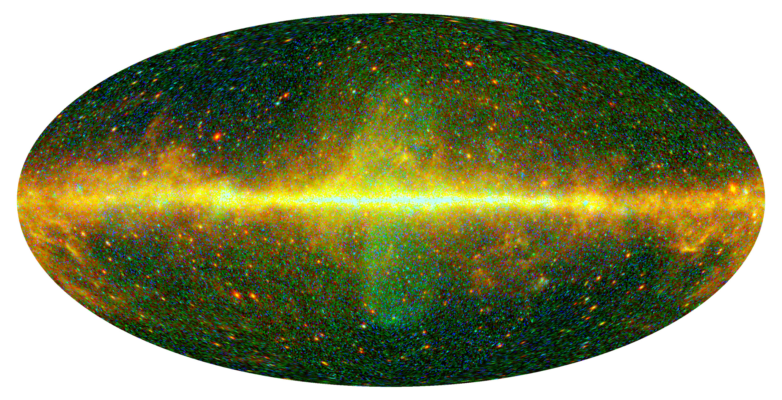
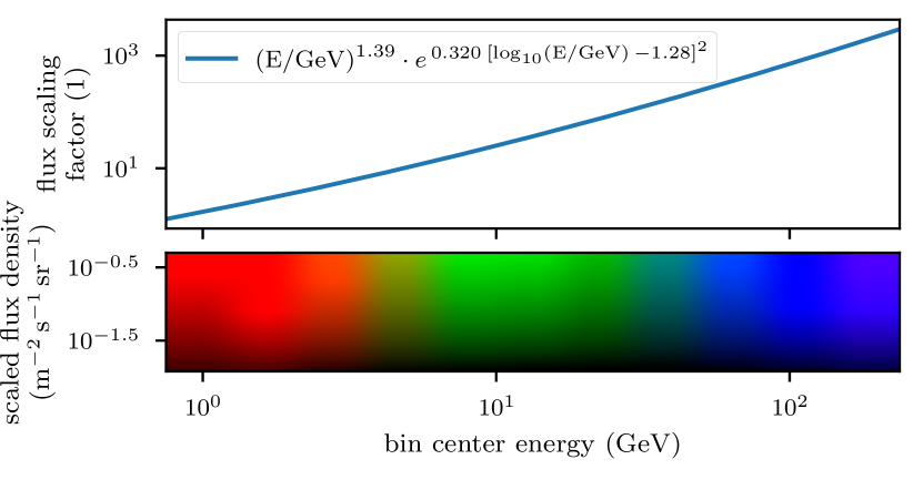
Figure 2: Introduction to the spatio-spectral plotting and corresponding data plot. Top: Exposure- and effective-area-corrected photon count observed by the Fermi LAT in the 1–316 GeV range within the selected time frame. The photon energies are color coded with red for the lowest and blue for the highest energies. To compensate for the flux intensity change within the shown energy range, we scaled the fluxes with an energy-dependent factor before plotting. This presentation is optimized to show spectral variations. Appendix C details the employed processing steps. For reading flux values at specific energies, the reader is referred to the public release of data products at the Zenodo data repository linked in the title footnote. This and all further sky maps are based on the HEALPix pixelization (Gorski et al. 2005) with an $\mathtt{nside}$ of 128 and employ the Mollweide projection. Middle: Energy-dependent flux scaling factor used for the spatio-spectral plotting. Bottom: Mapping of photon energies and scaled flux densities to perceived colors used in the spatio-spectral plotting.

3 Results

In the following, we present the results of applying the two imaging models M1 and M2 to Fermi LAT data and perform analyses to connect our findings with results from the literature. First, we look at the results of both models independently, and then perform comparative analyses.

3.1 Template-free spatio-spectral imaging via M1

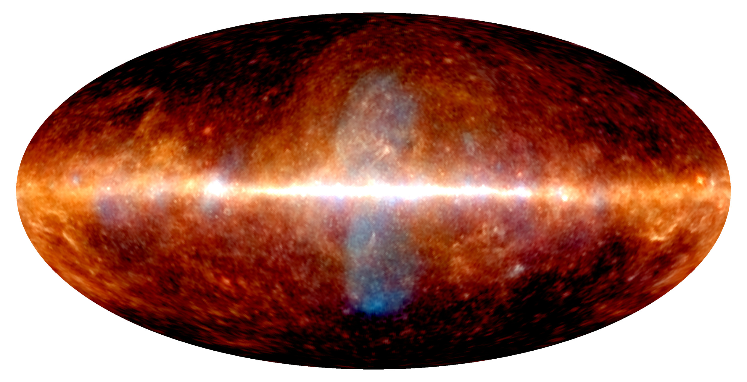
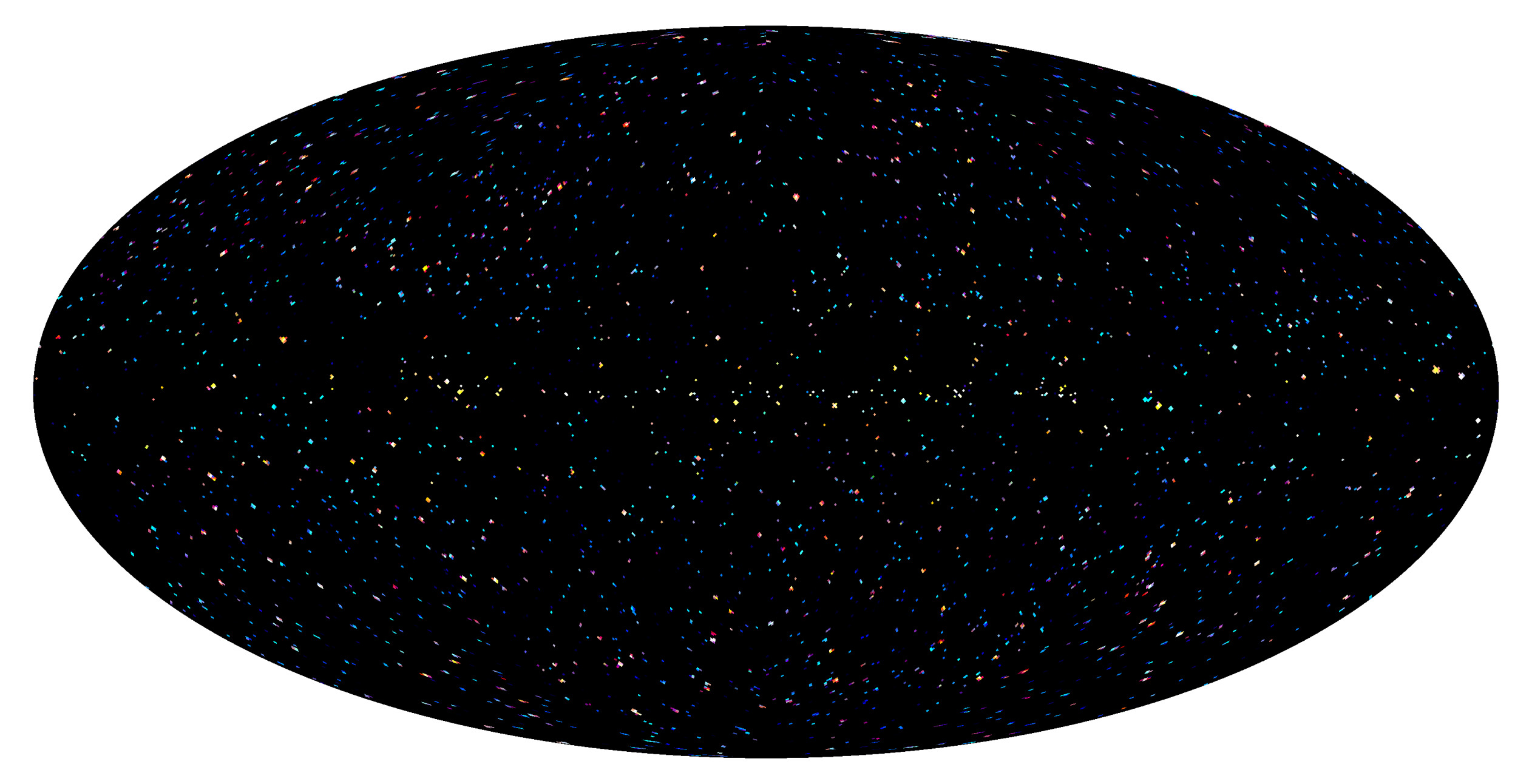
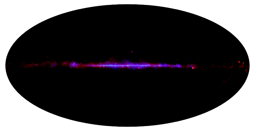
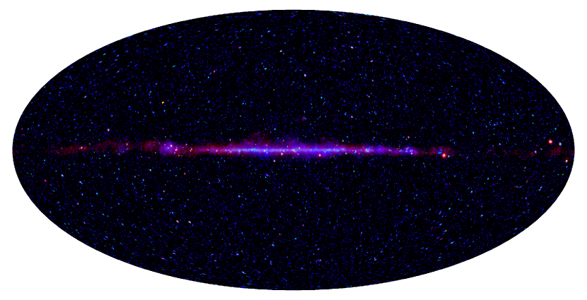
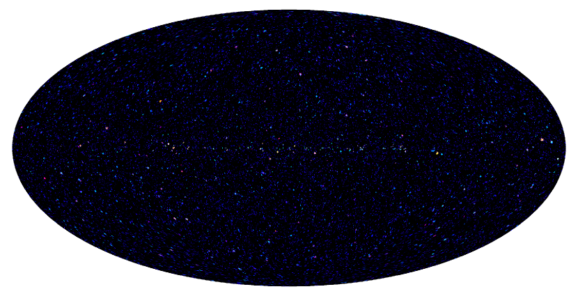
Figure 3: Results of the template-free reconstruction based on model M1. The figure uses the spectral domain color mapping introduced in the caption of Fig. 2 and Appendix C. It highlights spectral variations in the reconstructed skies. The color scale is provided in the bottom panel of Fig. 2. First row: Reconstructed gamma-ray sky. Second row: Separated diffuse emission (left) and PS sky (right). Third row: Absolute uncertainties of the diffuse component (left), the full gamma-ray sky (middle), and the PS component (right). The maps follow a Mollweide projection. Single energy bin maps of the diffuse emission component are provided in Fig. 24.

The spatio-spectral gamma-ray sky according to our template-free model M1 and its decomposition in diffuse and point-like flux components are shown in Fig. 3. With respect to the exposure- and effective-area-corrected photon count map shown in Fig. 2, the shot noise and point spread introduced by the measurement process are significantly reduced.

The reconstructed maps provide a detailed view of the gamma-ray sky, including spectral variations in the reconstructed diffuse emission and the PSs. The FBs are visible as gray and blue structures north and south of the GC, behind a strong foreground of hadronic emission, appearing orange in the maps. Visually comparing the Fig. 3 all-sky maps with the D³PO single-energy-band-based imaging results (Selig et al. 2015), the methodological progenitor of this work, we recognize a similar sky morphology, but also a near elimination of image artifacts associated with the bright Galactic disk exhibited by the D³P0 reconstructions.

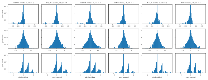
Figure 4: Selected residual histograms for the M1 reconstruction. The rows show all data bins for the energies 1.00–1.78 GeV (top), 10.0–17.8 GeV (middle), and 178–316 GeV (bottom). Fig. 25 shows the distribution of photon counts in the corresponding data bins. Pixel counts are shown on a logarithmic scale.

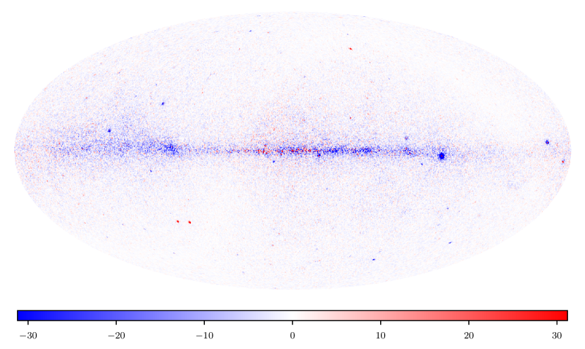
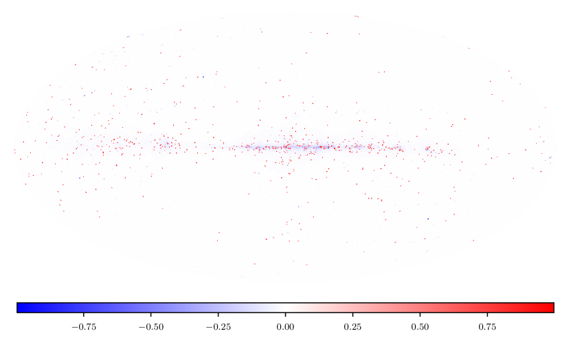
Figure 5: Selected residual maps for the M1 reconstruction, shown for the data bin with $\cos(\theta_{\mathrm{w^{\prime}}})\in(0.9,1.0]$ ($\mathrm{ct\_idx}=7$ in Fig. 4). Top: FRONT events. Bottom: BACK events. The energy bins are the same as in Fig. 4 but shown from left to right: 1.00–1.78 GeV (left), 10.0–17.8 GeV (middle), and 178–316 GeV (right). The maps are clipped to the 99.9th percentile of the residual amplitude in their respective energy bin. For comparison, Fig. 25 shows the distribution of photon counts in the selected data bins.

To evaluate the quality of fit, we calculated reduced $\chi^{2}$ statistics for the data bins, wherein we used our model’s flux prediction as the expected residual variance in each spatio-spectral voxel. For FRONT events, this yields an average reduced $\chi^{2}$ statistic of $1.1$, while for back events we find an average value of $0.9$.

Figure 4 shows residual histograms of selected data bins, with representative energy bins chosen from the reconstructed energy range. Residuals were calculated as $\,d_{\mathrm{\,vw^{\prime}i^{\prime}j^{\prime}}}-\lambda_{\mathrm{\,vw^{\prime}i^{\prime}j^{\prime}}}(I_{\mathrm{ij}})$. The residual distributions are consistent within the individual energy bins, but show strongly varying widths across the energy domain. This is expected, as with increasing photon energy, the photon count strongly decreases (see Fig. 1). The Poisson count distribution (Eq. 2) assumed for the data predicts residual variances equal to the expected photon count. Correspondingly, the likelihood permitted much larger residuals at high observed photon counts than at low observed photon counts. In the highest energy bin, the discrete nature of the photon count becomes apparent, and our model predicts count values slightly above full integer count values, leading to the stepped appearance of the 178–316 GeV residual histograms. This means our reconstructions in the highest spectral bins are partially driven by counts in the medium and low energy bins via spectral extrapolation based on the a priori spectral continuity built into our models.

Figure 5 shows spatial maps of residuals in selected data bins, corresponding to the third and sixth row in Fig. 4. The first column (1.00–1.75 GeV) shows an interesting pattern: in the locations of bright PSs, both the FRONT (top) and BACK (bottom) maps show large residuals, but with opposing signs. Where in the FRONT event residual map the central pixel of these PS driven residuals is positive and the surrounding pixel residuals are negative, the inverse pattern can be observed in the BACK event residual map. This indicates a PSF mismodeling, where for FRONT events the true point spread is weaker than modeled, while for BACK events, the true point spread is stronger than modeled. We believe this is also the reason for the mismatch in reduced $\chi^{2}$ statistics between FRONT and BACK events observed. We note that the Galactic ridge shows strong residuals in all shown maps. This again is related to the observation that residual variance is expected to be proportional to the photon flux, meaning high flux regions such as the Galactic ridge are expected to have larger residuals than the remainder of the sky. Besides this, the residual maps and histograms show a slight systematic mismodeling of the FBs in the shown medium energy bin (10.0–17.8 GeV), although only on the order of a fraction of a count. We conclude that besides the apparent PSF mismodeling, a good quality of fit was achieved.

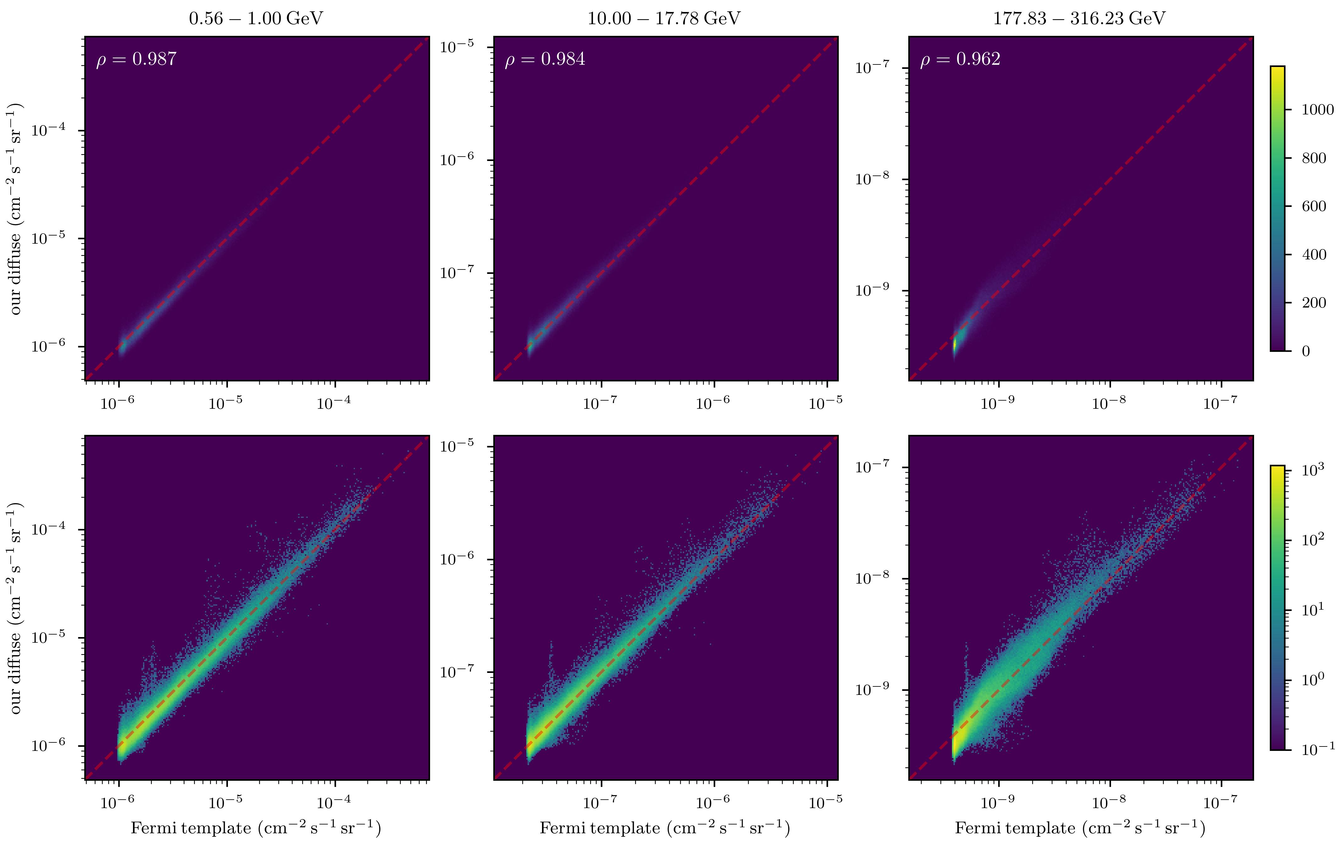
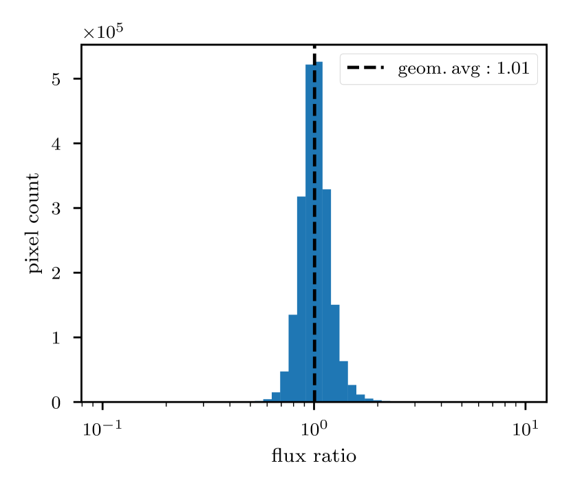
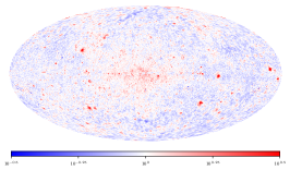
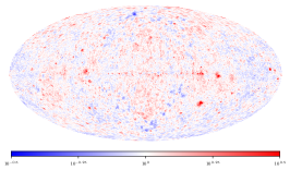
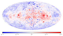
Figure 6: Comparison of the M1 diffuse reconstruction with the diffuse emission templates published by the Fermi Collaboration (diffuse foreground: gll_iem_v07, isotropic background: iso_P8R3_SOURCE_V3_v1). Top Left: 2D histograms of the diffuse flux found by our M1 reconstruction vs. the diffuse emission templates for the energy bins 0.56–1.00 GeV, 10.0–17.8 GeV, and 178–316 GeV. The histogram bins are logarithmically spaced in both fluxes. The top row shows the histogram counts with a linear color scale, while the bottom row shows them with a logarithmic color scale. The Pearson correlation between the template and our reconstruction on log-log scale, $\rho$, within the shown energy bins is given in the top column panels. The red dashed line marks perfect agreement. Top Right: Histogram of flux ratios (our diffuse reconstruction divided by the corresponding voxel values given by the template) for all spatio-spectral bins. Flux ratios are binned and displayed on a logarithmic scale. Bottom row: Flux ratio maps for the 0.56–1.00 GeV, 10.0–17.8 GeV, and 178–316 GeV energy bins with a logarithmic color scale. Numbers larger than $10^{0}$ ($=1$) indicate we reconstructed more flux than the template predicts, and vice versa.

To demonstrate our model is able to capture the full dynamic range of the diffuse gamma-ray sky, Fig 6 shows a comparison of the diffuse reconstruction via model M1 with the diffuse emission templates developed by the Fermi Collaboration in preparation of the fourth Fermi point source catalog (4FGL; Abdollahi et al. 2020). Overall, we observe a strong agreement of our diffuse reconstruction with the template, with increasing deviation in the high-energy limit. As the flux ratio histogram in the top-right panel of Fig 6 shows, the majority of spatio-spectral voxels have flux ratios in the interval $[0.8,1.25]$ and are distributed symmetrically around the geometric mean of flux ratios, $1.01$, which is very close to unity. We observe a geometric standard deviation of 17.5 percent.

The 2D histograms in the top-left panel of Fig 6 show our reconstructions follow a linear relationship with the template on log-log scales, with an average Pearson correlation coefficient of $\left<\rho\right>=0.98$. Toward lower flux intensities in each energy bin, the correlation weakens slightly, which is visible in the 2D histograms. In the 178–316 GeV energy bin, we observe a decreased correlation ($rho=0.96$) with the templates. This stems from flux deviations in pixels with medium to low flux (with reference to the flux values found in this energy bin). In this low flux regime, the Fermi templates predict more flux than we have reconstructed. This is driven by the isotropic background template, which imprints itself as a hard lower cutoff for the template flux values. The apparent flux cutoff is three times higher than the lowest value we reconstruct in this energy bin. A similar cutoff is also present in the 0.56–1.00 GeV and 10.0–17.8 GeV bins, but it differs only by $30\%$ from the lowest values we find in our reconstruction.

The bottom row of Fig 6 displays flux ratio maps between our diffuse reconstruction and the templates, calculated as $\mathrm{I}^{\mathrm{\>diff}}/\mathrm{I}^{\mathrm{fermi\>templates}}$, for the same energy bins as used in the 2D histograms. Areas of flux over-assignment with respect to the templates are shown in red, while areas of under-assignment are shown in blue. Over-assignment is most prominent in the locations of extended sources, which our diffuse reconstruction includes but whose emissions are not included in the templates. In the highest energy bin shown (178–316 GeV) the deviation between our reconstruction and the template is markedly stronger than in the two other energy bins, consistent with the observations above. In an elliptic region centered on the GC, reaching to high Galactic latitudes ($|b|\lesssim$ 80°) and longitudes of $|\ell|\lesssim$ 60°, we observe a strong but irregular pattern of deviations with a characteristic length scale of approximately 5°. East and west of this centered on the Galactic plane are regions of slight flux over-prediction with respect to the template, visible in red and reaching to Galactic latitudes of $|b|\lesssim$ 30°. At large Galactic latitudes and in the Galactic anticenter, we find on average approximately 20 percent less flux than the templates assume.

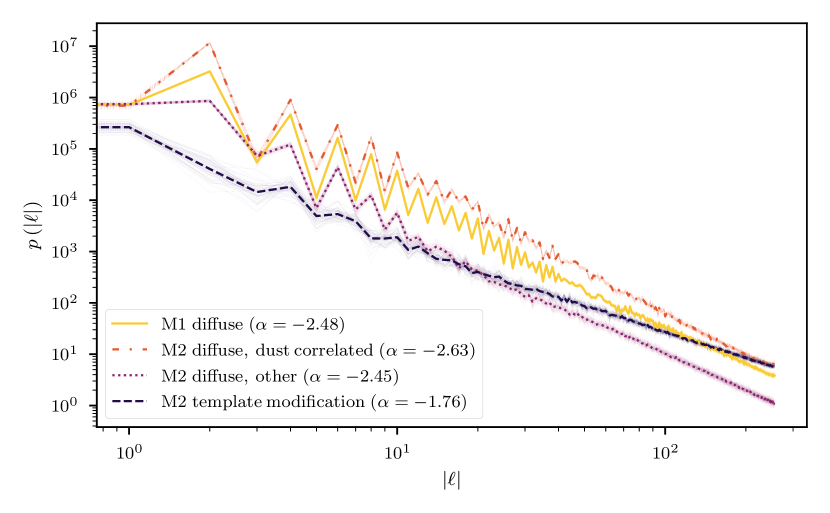
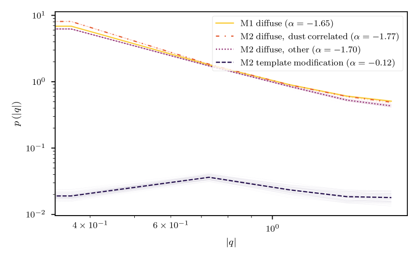
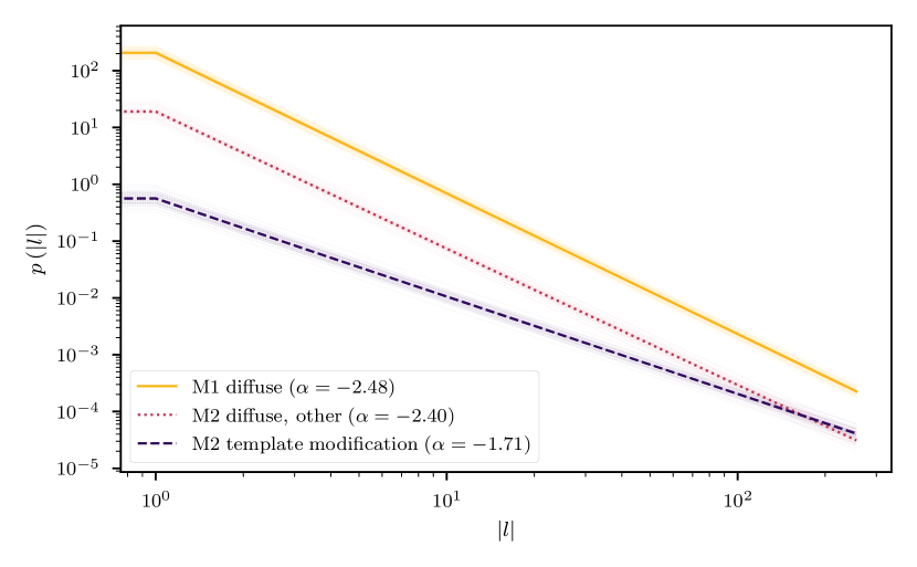
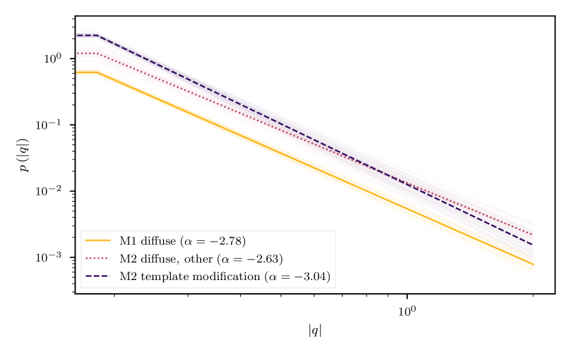
Figure 7: Power spectrum results of the two reconstruction runs. Top row: Empirical power spectra calculated directly from the reconstructed sky components (on log10 scale). Bottom row: Posterior power spectrum models of the correlated field models representing the $\tau^{\mathrm{\>c}}$. Left column: Angular power spectra. Right column: Energy spectrum power spectra. Bold lines show the geometric posterior sample means, while thin lines show individual posterior samples. All power spectra are plotted on log-log scale.

A significant quantity in our modeling of the sky are the spatial (angular) and spectral correlation power spectra (CPSs). As detailed in Sect. 2.3, the generative models for the $\tau^{\mathrm{\>c}}$ fields (here $\tau^{\mathrm{\>diff}}$) contain CPS models that provide self-consistent regularization for them and allow us to formulate prior knowledge of their spatial and spectral correlation structures $C^{\mathrm{\>c}}(\Delta x)$ and $D^{\mathrm{\>c}}(\Delta y)$. Figure 7 shows both the empirical CPSs of the reconstructed component maps (upper row) and the internal CPS models used in the correlated fields $\tau^{\mathrm{\>c}}$ (bottom row). For the M1-based diffuse reconstruction, we find a (posterior mean) empirical APS index of $-2.48$ and a (posterior mean) empirical energy spectrum power spectrum (EPS) index of $-1.65$. The empirical APS shows a zigzag pattern in the lower even and odd multipoles, which is a spectral imprint of the bright Galactic disk, exciting even angular modes stronger than odd ones. This pattern wanes toward smaller angular scales, as expected, as small angular scale structures exist in almost all regions of the sky.

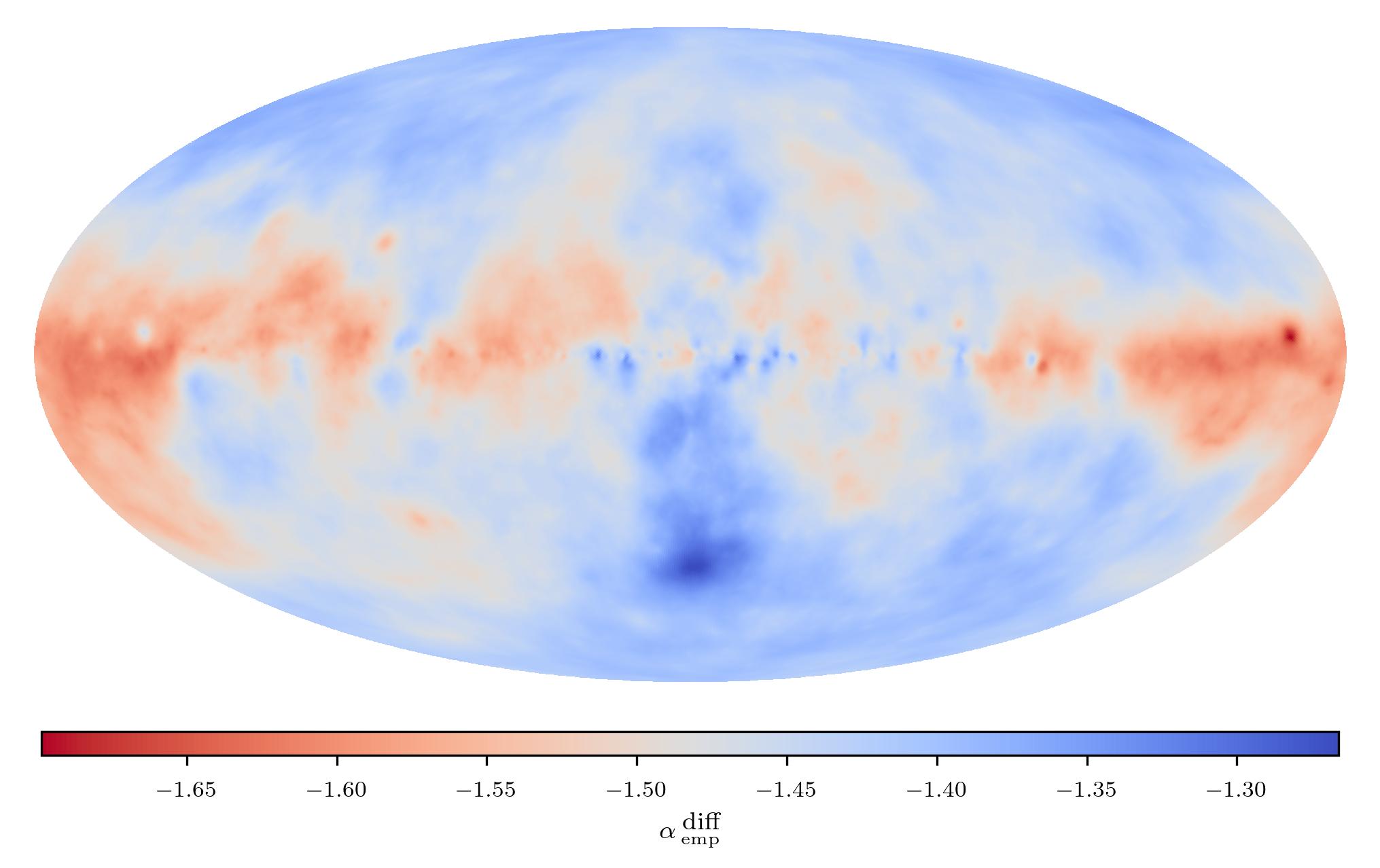
Figure 8: Empirical M1 diffuse spectral index map posterior mean, obtained by power-law fits to the diffuse emission component samples provided by the M1 reconstruction and subsequent averaging. Because we reconstruct fluxes integrated over logarithmically equidistant energy bins, spectral index values are offset by $+1$ with respect to un-integrated energy spectra (see Eqs. 3 and 4 in Sect. 2.1 for details).

The spatio-spectral imaging allows us to investigate a data-driven spectrum of the diffuse flux at all sky locations. To complement the qualitative spectral overview provided by the Fig. 3 spatio-spectral maps, we performed a pixel-wise power-law fit to the reconstructed diffuse sky energy spectra, resulting in the empirical spectral index map shown in Fig. 8. We remind the reader that we have reconstructed fluxes integrated within logarithmically equidistant energy bins, which exhibit energy spectral indices offset by $+1$ compared to nonintegrated fluxes (see Eq. 4). The empirical spectral index of the diffuse emission shown in Fig. 8 varies slowly across the sky, with the exception of a few small-scale structures discussed below. In regions dominated by neutral pion decay emission originating from the dense ISM, empirical spectral indices $\alpha^{\mathrm{\>diff}}_{\mathrm{\,emp}}$ in the range $\left[-1.65,-1.50\right]$ can be observed, appearing in red shades in the figure. In the region inhabited by the FBs, flatter spectra were found, with empirical spectral indices in the range of $\left[-1.45,-1.26\right]$, with a significant spectral hardening toward the tip of the southern bubble, appearing in blue. In regions where the Galactic foregrounds are weak, a spectral index around $-1.40$ is observed. In the outer Galaxy, the Galactic plane is permeated by regions with spectral indices between $-1.45$ and $-1.40$, suggestive of outflows of relativistic plasma from the Galactic disk. In the Fig. 3, these are visible as white veils above the remaining emission. Regarding small-scale structures, we note multiple strongly localized hard spectrum regions in the Galactic disk, close to the GC, with a spectral indices in the $\left[-1.35,-1.26\right]$ range. The region surrounding the Geminga pulsar shows an average spectral index of $-1.70$, making it the region with the lowest spectral index in this map.

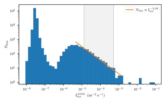
Figure 9: PS pixel count histogram for the M1 reconstruction on log-log scale. The orange line shows a power-law fit to the brightness distribution in the brightness range highlighted in gray. Flux values below $5\cdot{10}^{-7}$ $\mathrm{m}^{-2}\,\mathrm{s}^{-1}$ should be regarded as non-detections. The distribution function in that area is prior-driven.

We now turn to the analysis of the PS results made with the M1 model. As described in Sect. 2.3, we used a fixed PS brightness prior that follows a power law with index $-2.5$ for large brightness values and has an exponential cutoff for low brightness values, with the prior mean set to lie two orders of magnitude below the expected diffuse emission brightness mean. Figure 9 shows the posterior PS pixel brightness distribution found with model M1. In it, three distinct populations of PS pixels can be seen:

First, the majority of PS pixels exhibit a posterior mean brightness at the low end of the brightness scale between ${10}^{-8}$ and ${10}^{-7}$ $\mathrm{m}^{-2}\,\mathrm{s}^{-1}$. These are PSs that were not “switched on” during the reconstruction, leaving their posterior brightness close to the prior mean. They should be regarded as non-detections of PS flux.

Second, between ${10}^{-6}$ and ${10}^{-3}$ $\mathrm{m}^{-2}\,\mathrm{s}^{-1}$, lies a population of PS pixels for which the data requested significant flux contributions. Their distribution matches the shape found for PS distributions in other works; Abdollahi et al. (2020, Fig. 15) provide the distributions found in the first to fourth source catalogs (1FGL – 4FGL) published by the Fermi Collaboration. The number of sources in this group falls off quickly below a pixel brightness of $2\cdot{10}^{-6}$ $\mathrm{m}^{-2}\,\mathrm{s}^{-1}$, giving the effective detection limit of our analysis. We perform a power-law fit to the found distribution in the range of ${10}^{-5}$ to $5\cdot{10}^{-4}$ $\mathrm{m}^{-2}\,\mathrm{s}^{-1}$, where the distribution follows a stable slope on log-log scales. We find a power law with index $-2.26$, which is close enough to the prior assumption of $-2.5$ that we do not expect strong biases in the estimated flux values within that range.

Third, a few isolated sources exhibit brightness values above ${10}^{-3}$ $\mathrm{m}^{-2}\,\mathrm{s}^{-1}$. These correspond to the brightest sources found, including the Vela and Geminga pulsar. We discuss these findings in the context of previous works in Sect. 4.

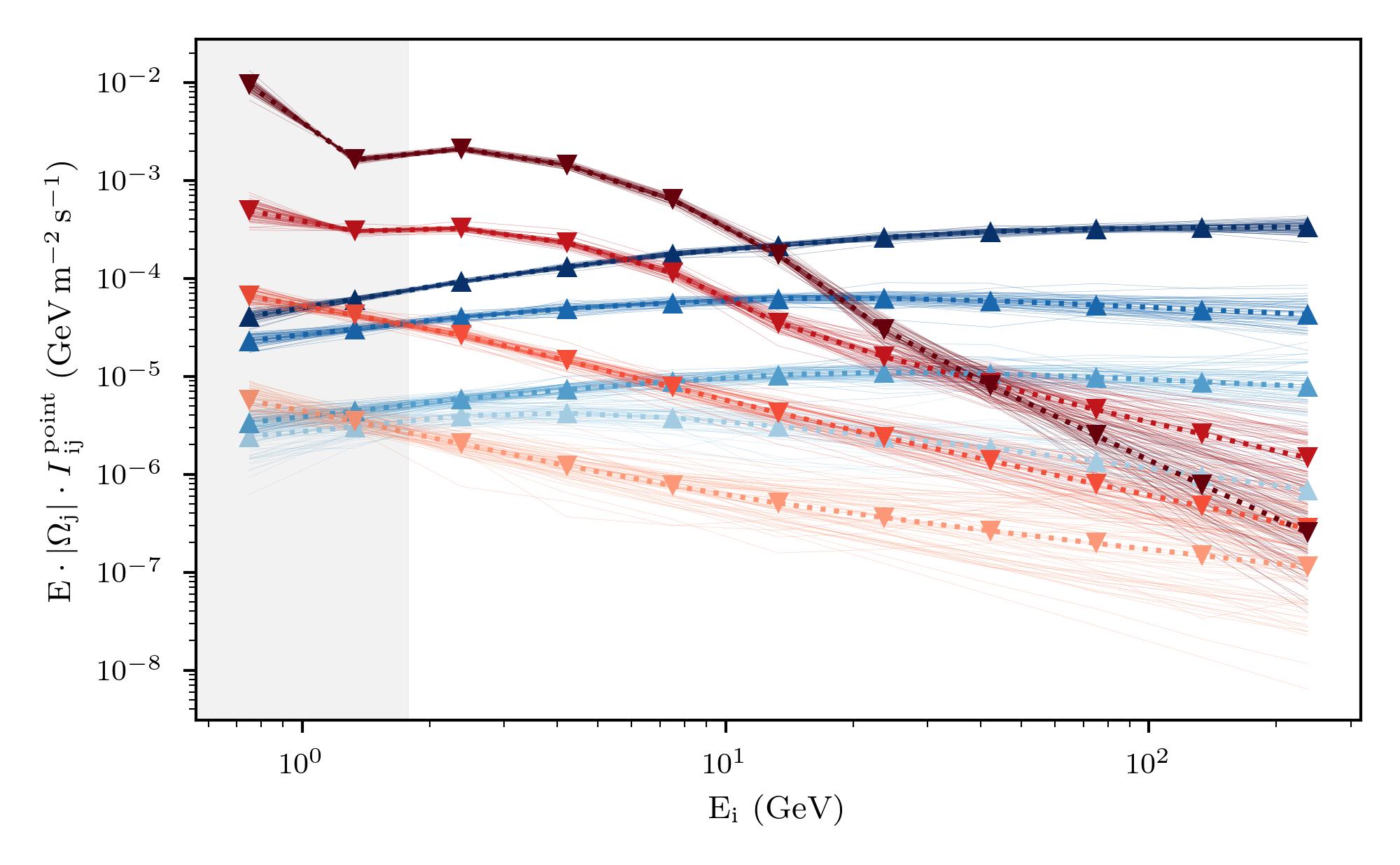
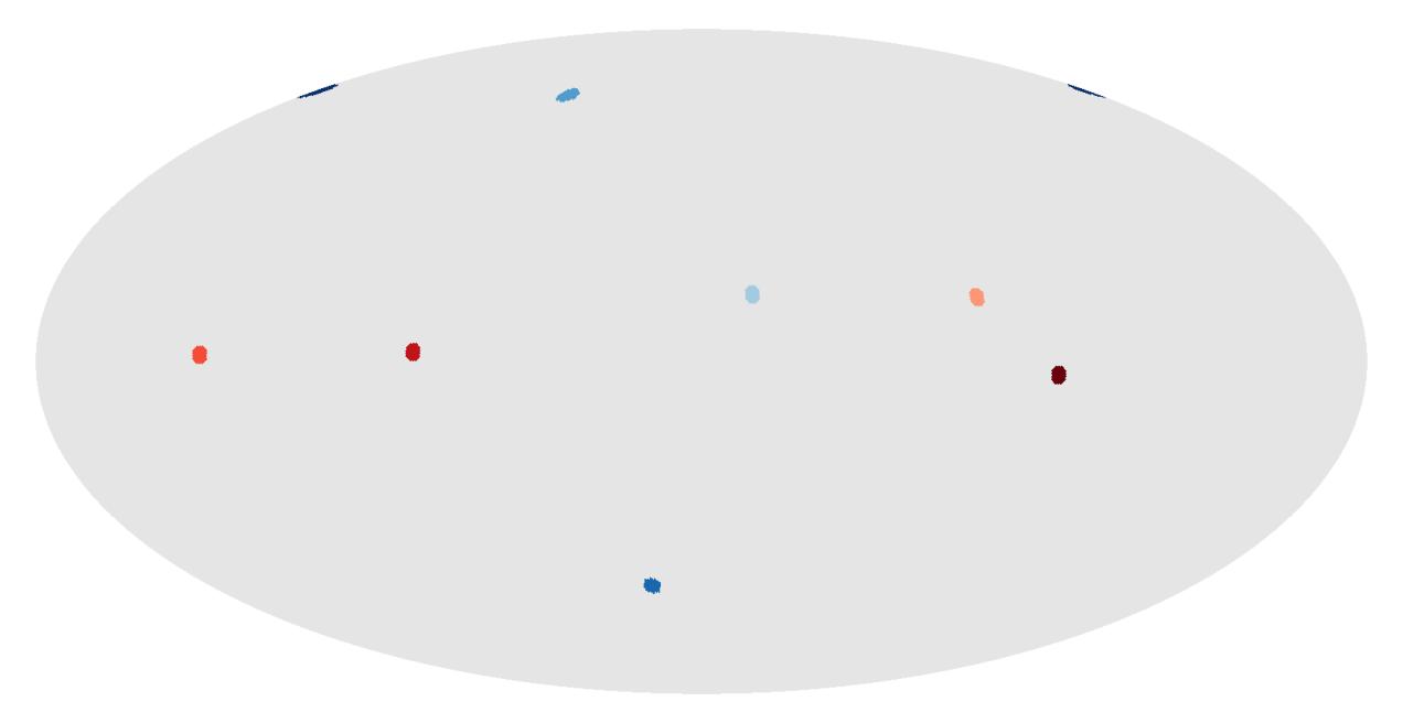
Figure 10: Reconstructed energy spectra of selected PS pixels based on model M1. The pixels were selected by sorting them by their geometric mean flux in the 1.00-1.77 GeV (red, down-pointing triangles) and 100-177 GeV energy bins (blue, up-pointing triangles) and then choosing the brightest, 10th, 100th, and 1000th brightest source in each of the two energy bins. Right: Positions of the selected PSs. Left: Corresponding energy spectra, matched by color. The triangle markers display the posterior geometric mean flux reconstructed for the sources in each energy bin, while the thin continuous lines show the posterior spectrum samples associated with sources. The spectra are plotted on log-log scale.

Continuing our analysis of the M1 PS results, we turn to the full reconstructed energy spectra of PSs. Figure 10 shows this for a few PSs, selected as the brightest, 10th, 100th, and 1000th brightest source in the 1.00-1.77 GeV and 100-177 GeV energy bins.

The reconstructed spectra deviate from pure power laws in energy, which would appear as straight lines in the graph. The spectrum of the brightest source pixel in the 1.00-1.77 GeV energy bin shows a spectral hump characteristic of hadronic emission and flattens to a straight line above 40 GeV. The same is true of the 10th brightest source in this bin, although its spectrum already flattens above 1 GeV. The sources have soft spectra with spectral indices below $-1.5$ and all lie within the Galactic plane (except for the faintest). The PSs selected in the 100-177 GeV energy bin all show comparatively straight energy spectra with a slight uniform bend to them. They all have harder spectra with spectral indices close to $-1.0$ and lie at high Galactic latitudes (except for the faintest, again).

As seen by the posterior sample variability in the graph, the posterior uncertainty generally increases toward higher energies and with decreasing source brightness. This is expected, as discussed above, because of low photon count at high energies and thus less informative data, and because of low intensity sources being “covered” by stronger diffuse emission, making their spectra less constrained by data than those of brighter sources.

Figure 10 also reveals that the spectral deconvolution is facing a problem at lower energies, which becomes most apparent for the steeper spectrum sources. Because of the large EDF spread at low energies, the data corresponding to the lowest reconstructed energy bin is contaminated by photons with true energies below its low energy boundary. Since the model has no representation of this, we excluded the data of the lowest reconstructed energy bin from our likelihood. This has the downside of making the lowest reconstructed energy bin under-informed compared to the higher energy bins. As it is only informed by photon counts from the second-lowest energy bin, errors in the EDF model or its numerical representation were imprinted onto the low energy end of the reconstruction without mitigation. We therefore recommend to exclude the lowest energy bin in analyses of the reconstruction results.

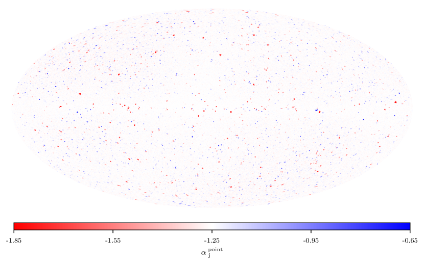
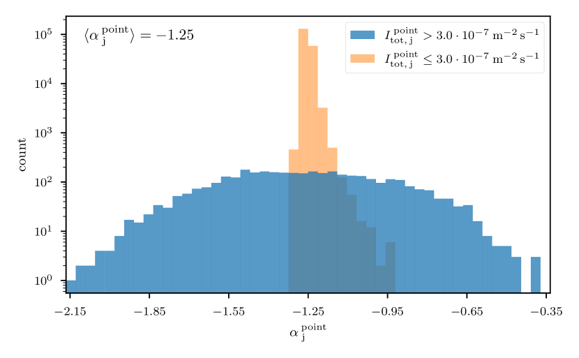
Figure 11: M1 PS spectral index $\alpha^{\mathrm{\>point}}_{\mathrm{j}}$ posterior means. We note that the spectral indices have an offset of $+1$ introduced by the logarithmic binning of the energy dimension (see Eq. 4). Left: Map of spectral indices recovered for the PS pixels. The color scale is centered on the prior mean, $-1.25$, and ranges from two prior standard deviations above to two standard deviations below the prior mean. Right: Histogram of posterior PS pixel spectral index means for switched on (blue) and switched off PS pixels (orange). The x-axis is centered on the prior mean, with the ticks indicating prior standard deviation sized steps from the prior mean. The y-axis shows counts on a logarithmic scale.

Taking a broader view at the whole population of reconstructed PSs, Fig. 11 shows the posterior mean of all sources’ spectral indices. As can be seen both from the left and right panel of the figure, most PS pixels do not deviate from the prior mean. This is mainly because of “switched off” source pixels, which strongly clusters around the spectral index prior mean of $-1.25$ (see the orange histogram in the right panel of Fig. 11). In contrast, the population of switched on PS pixels shows a broad distribution of posterior spectral indices ranging from $-2.15$ to $-0.35$ (see the blue histogram in the right panel of Fig. 11). It extends markedly beyond the limits observed for the diffuse emission ($-1.70$ to $-1.26$). For all source pixels, individual posterior mean spectral indices can be read off in the left panel of Fig. 11. Noteworthy sources include the Vela pulsar, for whose containing pixel we find a soft spectrum ($\alpha<-1.85$), and Vela-X, for whose containing pixel we find a hard spectrum ($\alpha>-0.95$).

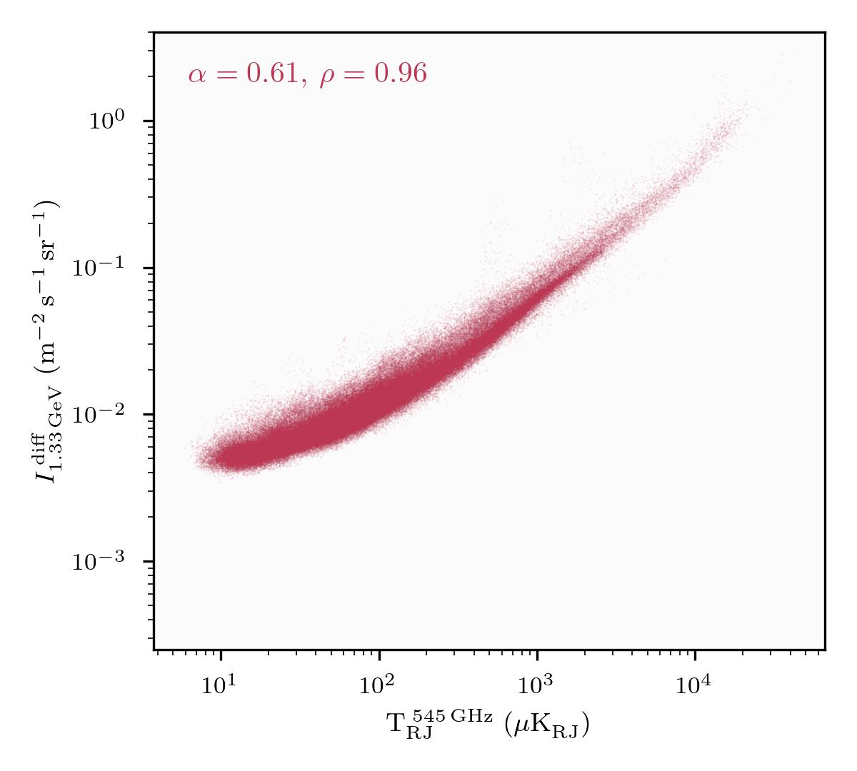
Figure 12: Scatter plot of the M1 diffuse flux density values in the 1.00-1.77 GeV energy bin against the Planck 545 GHz thermal dust emission map values. Each pixel is represented by a dot, with the x-axis showing the brightness temperature $\mathrm{T}_{\mathrm{RJ}}^{\>545\,\mathrm{GHz}}$ measured by Planck for this pixel and the y-axis showing the corresponding flux density value found by our reconstruction. Both quantities are shown on a logarithmic scale. The text in the upper left corner shows the slope of a linear fit to the dots, $\alpha$, and the Pearson correlation coefficient between the two maps on log-log scale, $\rho$.

Closing the results section of the template-free model M1, Fig. 12 shows a scatter plot of the diffuse reconstruction based on M1 against the Planck thermal dust emission map used as a template in model M2. Above diffuse gamma-ray fluxes of $3\cdot{10}^{-2}$ $\left(\mathrm{m}^{2}\,\mathrm{s}\,\mathrm{sr}\right)^{-1}$ we observe a close to linear scaling of the two quantities on log-log scale, corroborated by a high Pearson correlation coefficient of $\rho=0.96$. A linear fit between the logarithmic pixel values of the two maps yields a best-fit slope of $\alpha=0.61$. Below the stated flux limit, the correlation weakens, as other dust-independent emission processes begin contributing significant proportions of the diffuse emission. These emissions are unveiled in the template-informed reconstruction, where dust-correlated emission was taken up by the template-informed diffuse component and other flux is modeled with the second, free, diffuse component. The results of this are presented in the following section.

3.2 Template-informed spatio-spectral imaging via M2

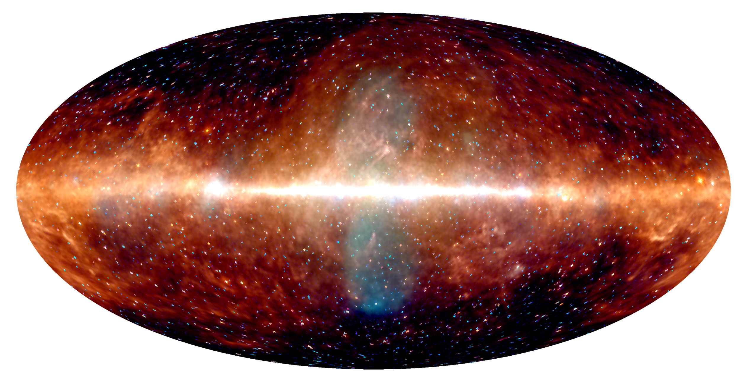
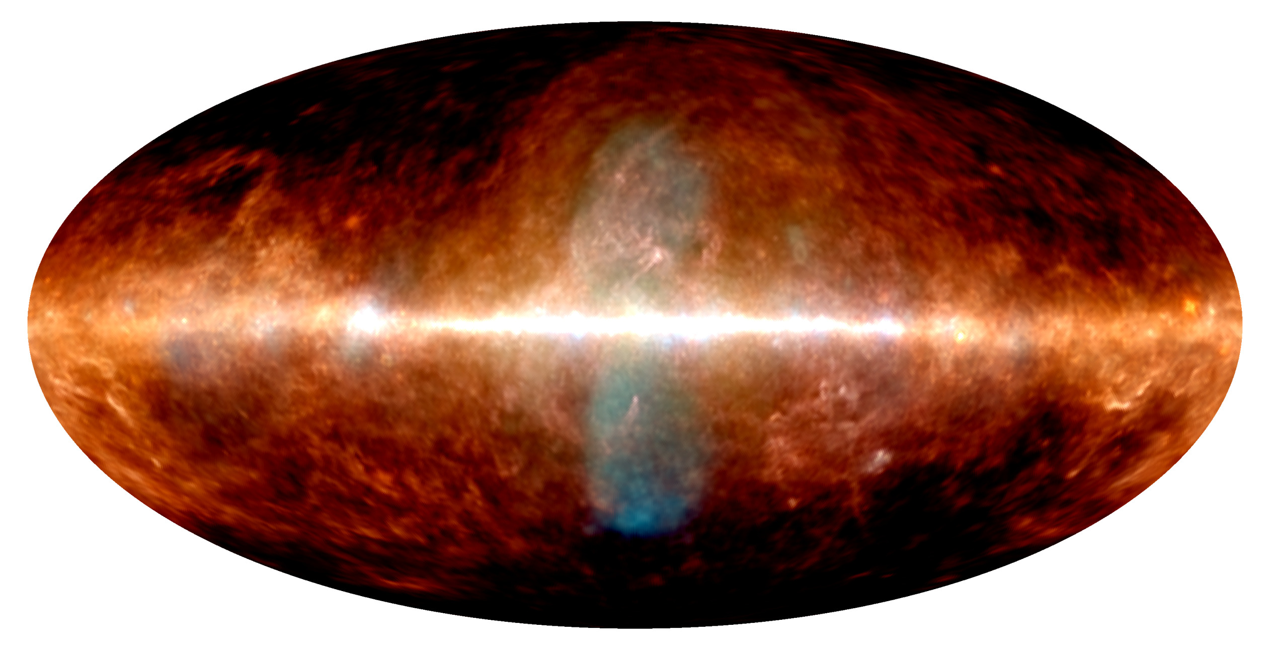
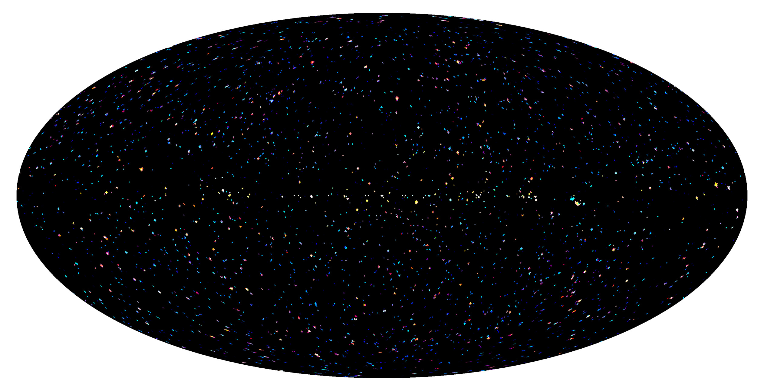
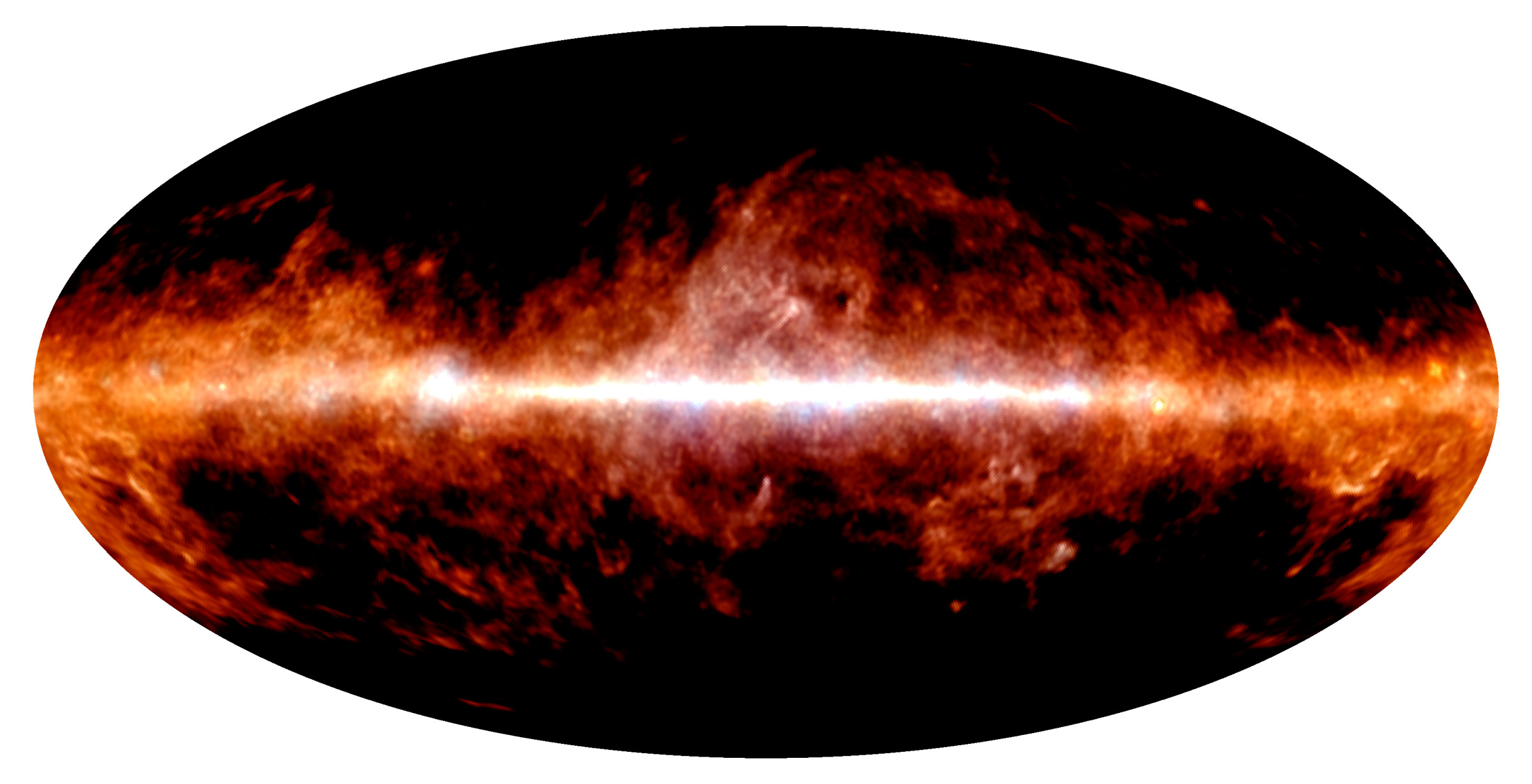
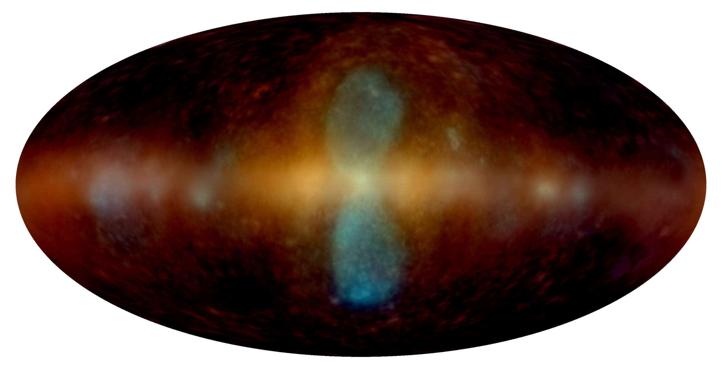
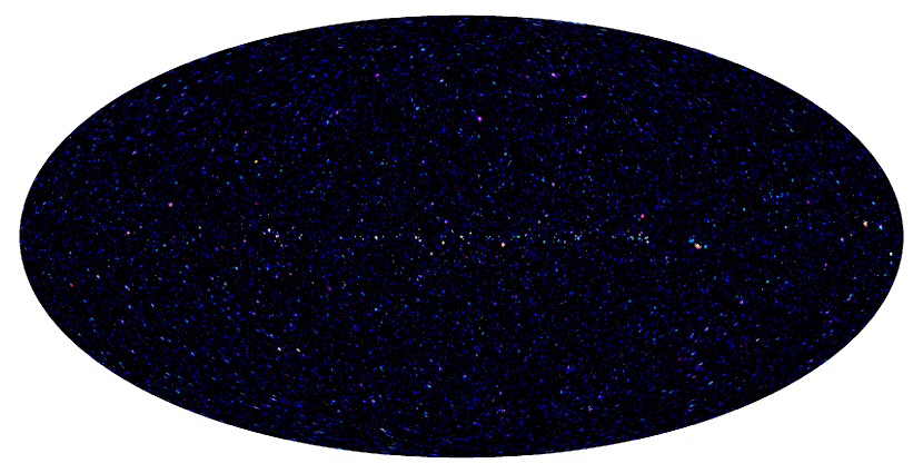
Figure 13: Results of the template-informed reconstruction based on model M2. The figure uses the spectral domain color mapping introduced in the caption of Fig. 2. The color scale is provided in the bottom panel of Fig. 2. First row: Reconstructed gamma-ray sky. Second row: Separated diffuse emission sum (left) and PS emissions (right). A rendering of the diffuse emission sum without color saturation enhancement is show in Fig. 30. Third row: Dust-correlated diffuse emissions (left) and other diffuse emissions (right). Fourth row: Posterior standard deviation of the sum of the diffuse emissions (left), the full sky (middle), and the PS emissions (right).

The spatio-spectral gamma-ray sky reconstruction according to our template-informed model M2 is shown in Fig. 13. Additional to the decomposition into point-like and diffuse emission, the M2 model allows us to further decompose the diffuse emission into a thermal dust emission correlated component and other diffuse emissions. Maps of the two diffuse components are shown in the third row of Fig. 13. Unveiled from the dust-correlated emission, the $I^{\mathrm{\>nd}}$ map (right) shows all dust-independent diffuse emission. First, this includes the FBs, as expected. Second, there appears a bright soft spectrum emission structure in the inner Galaxy, left and right of the FBs and symmetric around the north-south axis of the Galaxy. It traces the shape of the FBs to Galactic latitudes of $|\mathrm{b}|<$ 30° at a longitudinal distance of approximately 10° on the map and has a smooth appearance. Third, along the Galactic plane in the western hemisphere of the sky, there is a faint soft spectrum emission structure, also of smooth appearance. Lastly, there is a structure of small clumps of emission surrounding the FBs and extending to high Galactic latitudes in the northern hemisphere. Structures similar to this are also visible in the southern bubble, even in the M1 diffuse sky maps (Fig. 3). These might be part of the larger collection of small-structured emissions just mentioned or correspond to a internal structure of the bubble emissions.

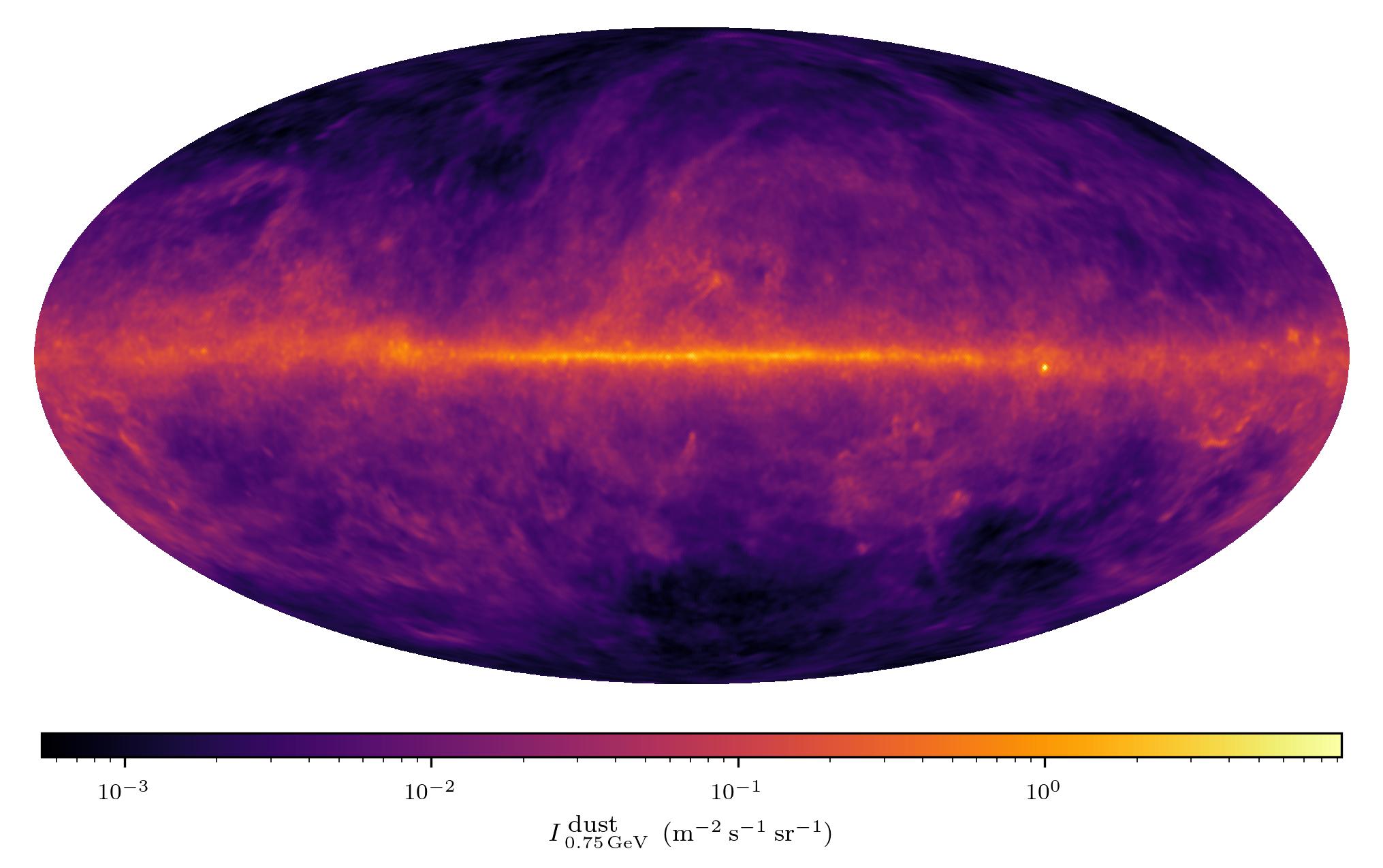
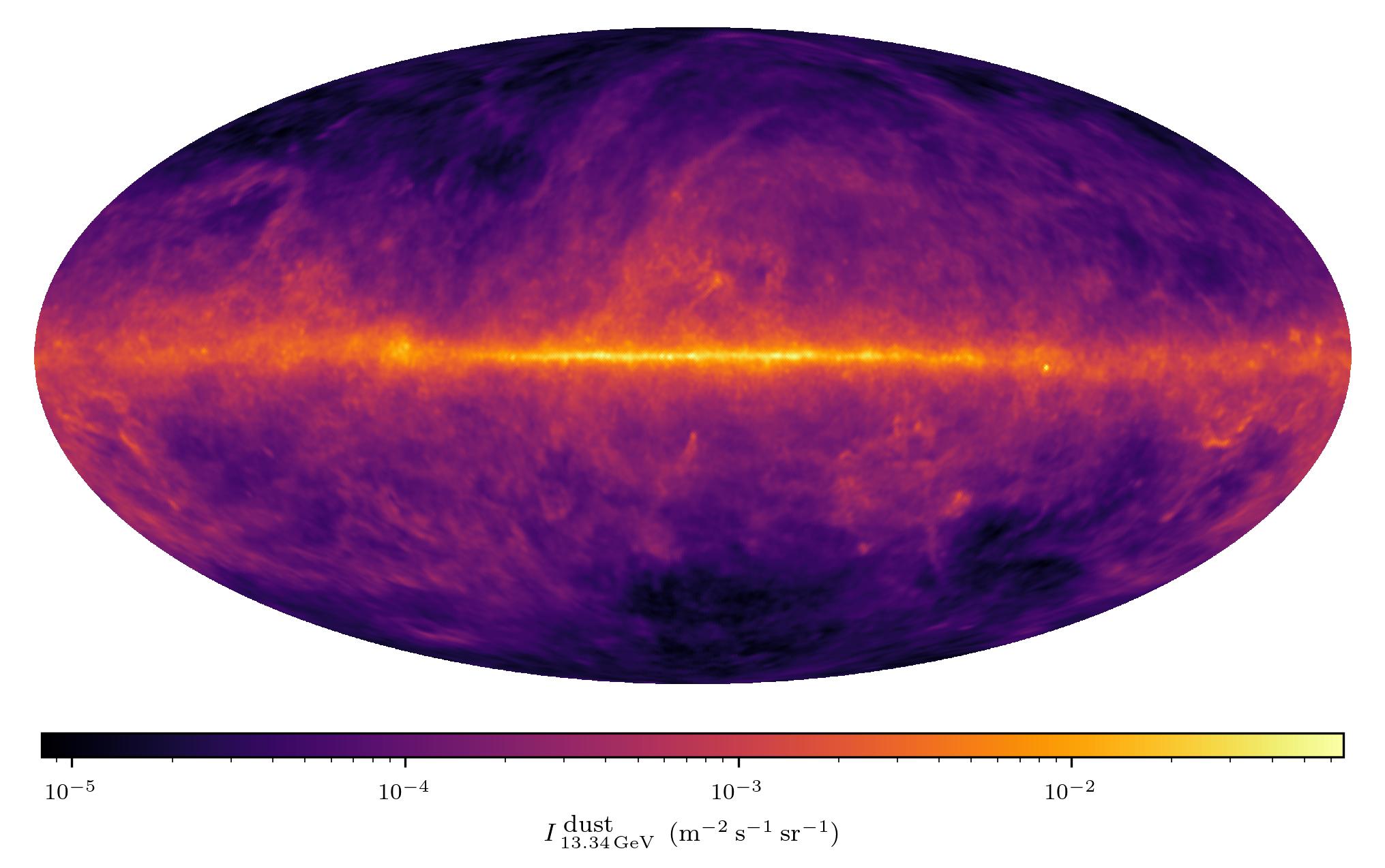
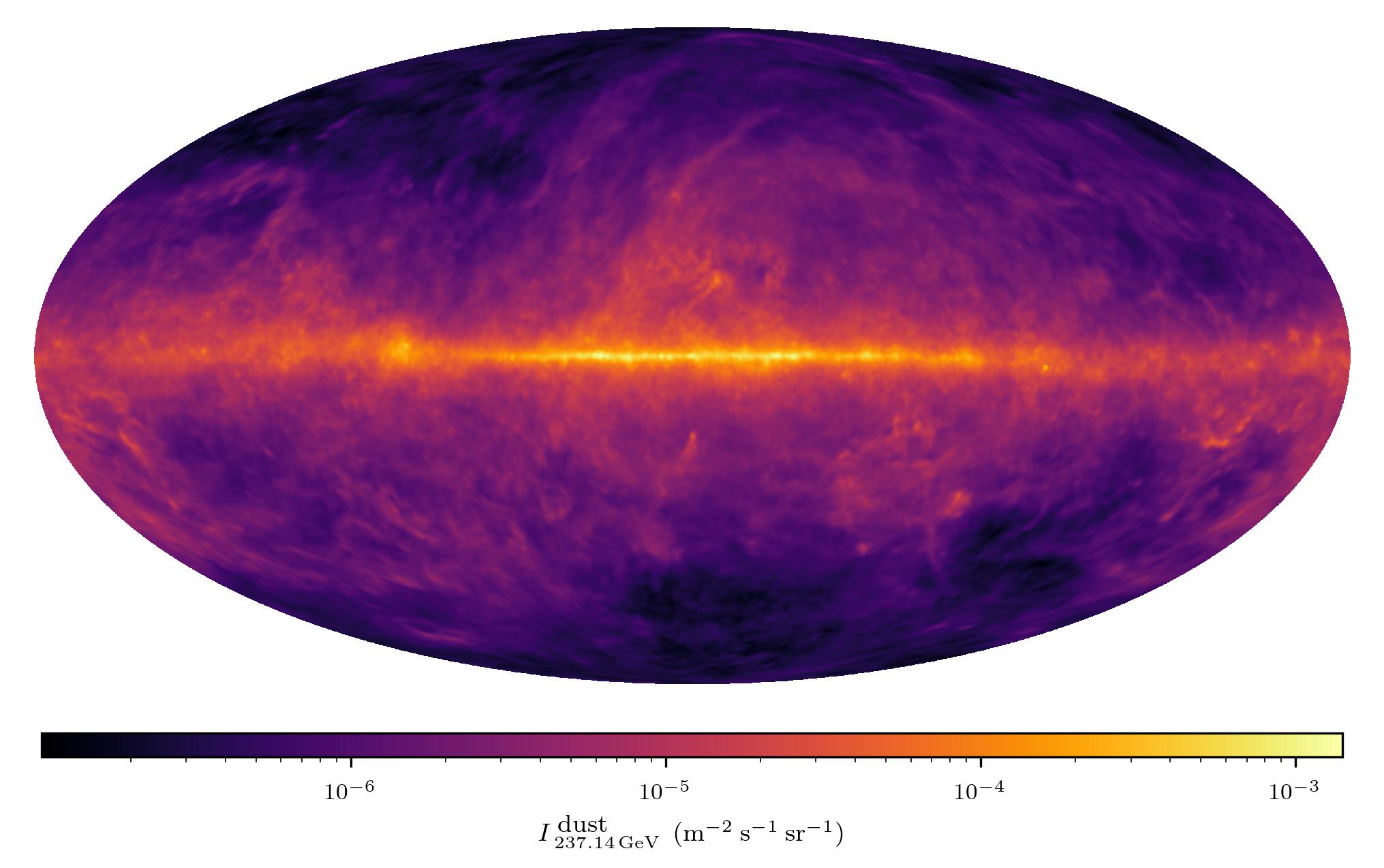
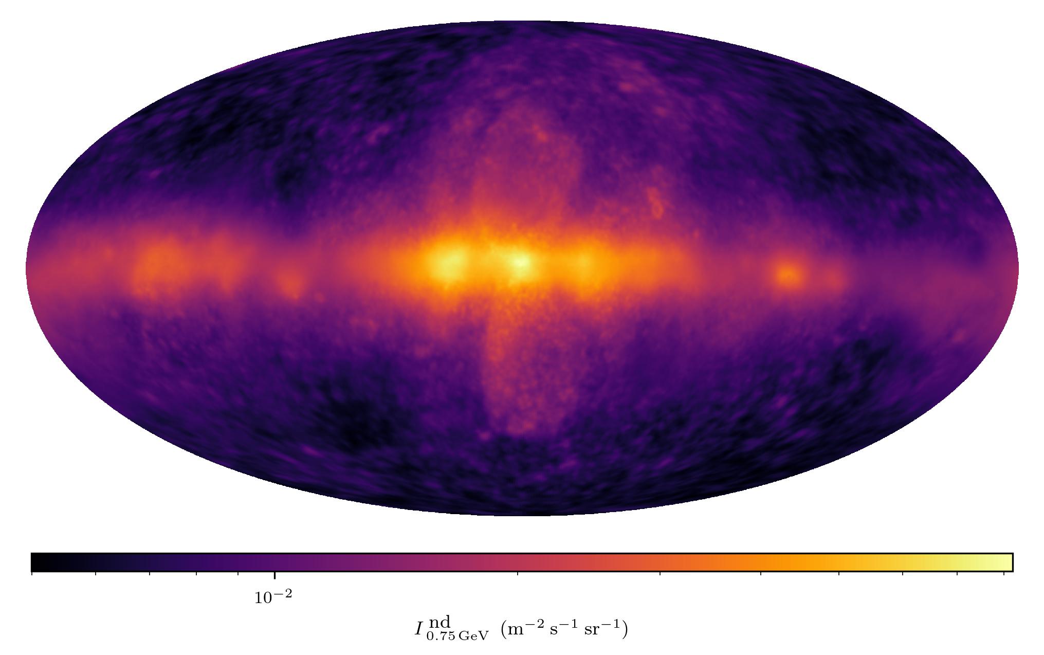
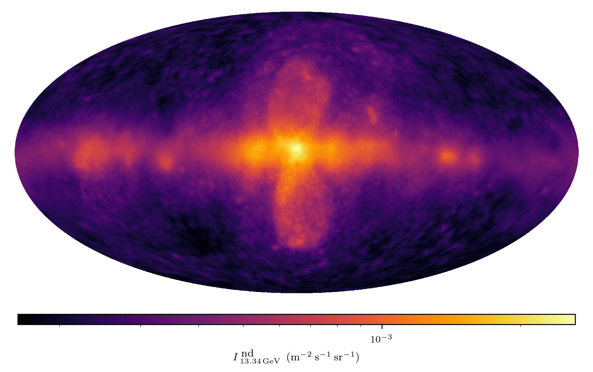
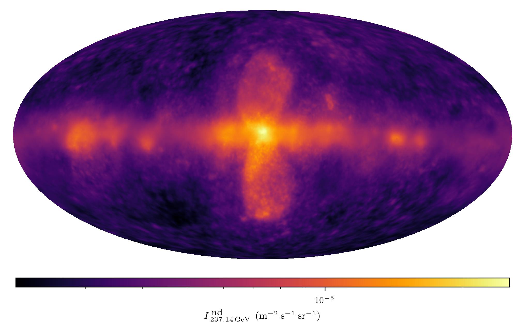
Figure 14: Single energy plots of the M2 diffuse components with a logarithmic color scale. Top row: Dust-correlated (template-informed) diffuse emission. Bottom row: A priori dust-independent (free) diffuse emission. Energy bins: 0.56–1.00 GeV (left), 10.0–17.8 GeV (middle), and 178–316 GeV (right). All panels have individual brightness scales and visualize the full dynamic range of their respective maps.

Figure 14 shows single energy bin plots of the two M2 diffuse component reconstructions. From the $I^{\mathrm{\>dust}}$ panels in the upper row, the large dynamic range of the dust-correlated emission reconstruction becomes apparent, which is induced by the thermal dust emission template. In the $I^{\mathrm{\>nd}}$ maps, the constellation of emission clumps surrounding the FBs can be seen to be part of a more continuous outer bubble structure, reminiscent of the X-ray arcs observed by eRosita (Predehl et al. 2020).

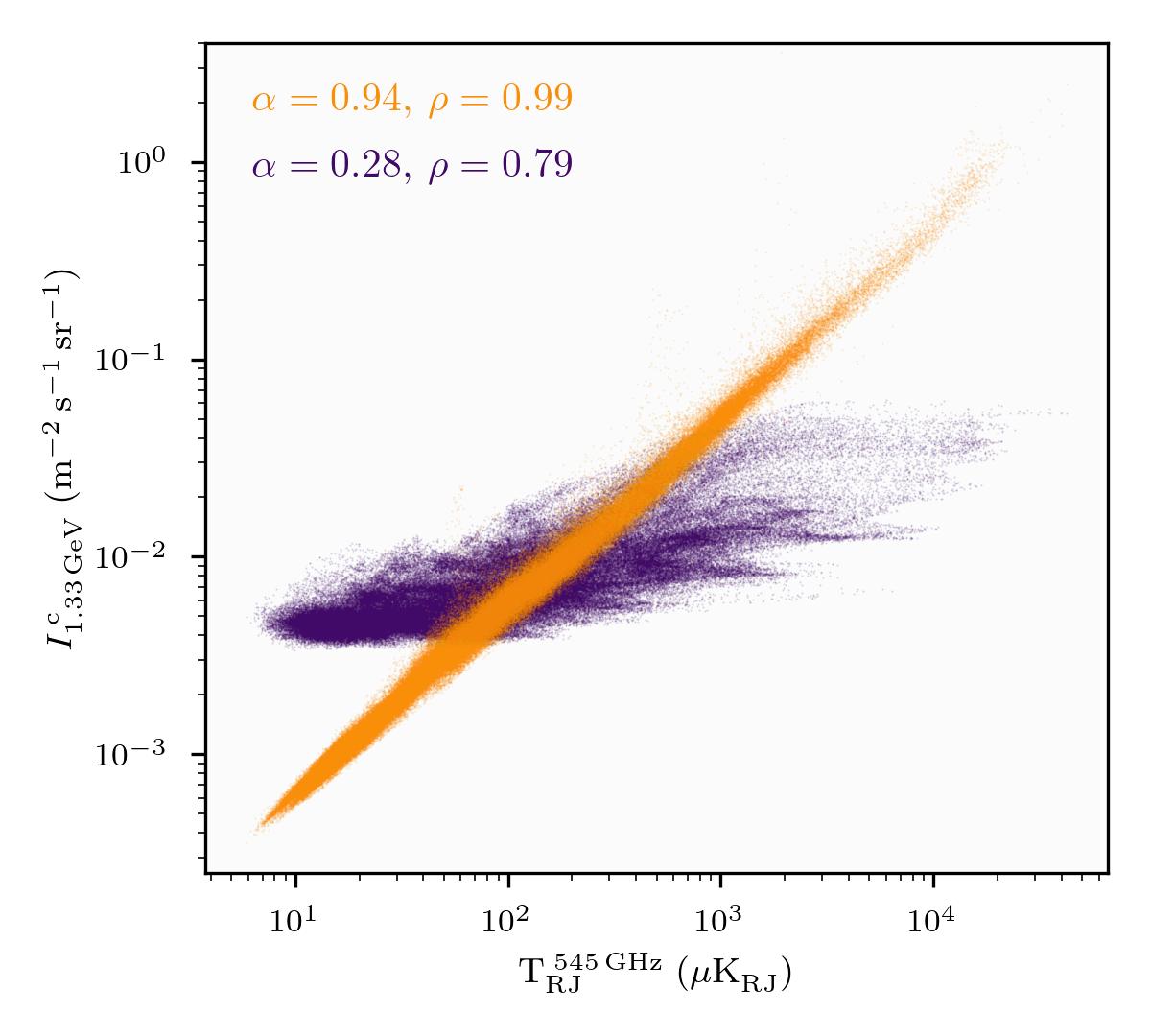
Figure 15: Scatter plot of the M2 diffuse flux density values in the 1.00-1.77 GeV energy bin against the Planck 545 GHz thermal dust emission map values. Each pixel is represented by a dot, with the x-axis showing the brightness temperature $\mathrm{T}_{\mathrm{RJ}}^{\>545\,\mathrm{GHz}}$ measured by Planck for this pixel and the y-axis showing the corresponding flux density value of our reconstruction. Both axes have a logarithmic scale. The points for the dust template informed diffuse component $I^{\mathrm{\>dust}}$ are shown in orange, while the points for the a priori dust-independent diffuse component $I^{\mathrm{\>nd}}$ are shown in purple. The text in the upper left corner shows the slope of a linear fit to the dots, $\alpha$, and the Pearson correlation coefficient between the thermal dust map and our reconstructions on log-log scale, $\rho$.

So far, we have assumed that the template-free diffuse emission component $I^{\mathrm{\>nd}}$ reconstructs dust-independent emissions. To test whether this assumption holds true, Fig. 15 shows a scatter plot of the M2 diffuse gamma-ray maps $I^{\mathrm{\>dust}}$ and $I^{\mathrm{\>nd}}$ with the Planck thermal brightness map. $I^{\mathrm{\>dust}}$ shows a strong linear relationship with the thermal brightness map on log-log scale ($\alpha=0.94$), while $I^{\mathrm{\>nd}}$ only has a weak linear relationship with it ($\alpha=0.28$). This indicates a good unmixing of the emission components. The same pattern, albeit less pronounced, is observed in the Pearson correlation coefficients on log-log scale with $\rho=0.99$ for $I^{\mathrm{\>dust}}$ and $\rho=0.79$ for $I^{\mathrm{\>nd}}$. The strong Pearson correlation of $I^{\mathrm{\>nd}}$ with the dust map indicates $I^{\mathrm{\>nd}}$ is dominated by ISM-tracing gamma-ray emissions.

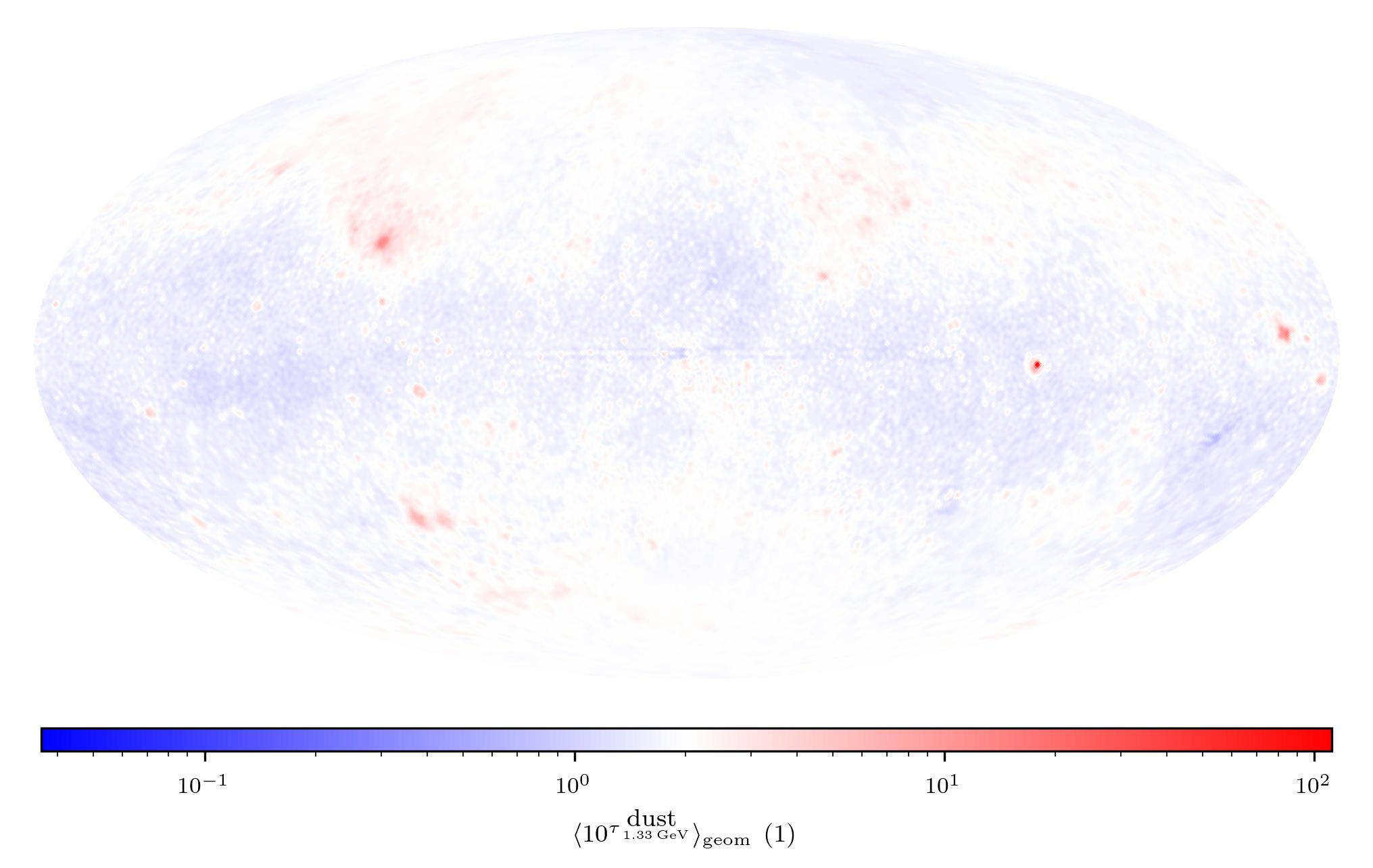
Figure 16: M2 multiplicative thermal dust template modification field for the 1.00-1.77 GeV energy bin (posterior geometric mean) on a logarithmic color scale. Fig. 27 shows the modification field maps for two additional energy bins and corresponding posterior uncertainty maps.

Figure 16 shows the dust template modification field $\tau^{\mathrm{\>dust}}$ in the energy bin from 1.00 to 1.77 GeV. It shows a median value of 2.0, indicating the brightness reference scale $I^{\mathrm{\>dust}}_{\mathrm{0}}$ was chosen too low by that factor. The strongest modifications can be seen in the regions of the Vela pulsar and nebula, the Geminga pulsar, the Crab pulsar and nebula, PSR J1836+5925, and the blazar 3C 454.3. All these are very bright PSs or extended objects, here contaminating the dust-correlated emission map. Besides this, the dust modification map of the energy bin only shows very little structure, with most values lying in the range of 1.0 – 3.0. One notable structure in the map is a sharp line along the Galactic plane, with modification field values around $2.0$ on the disk and slightly below $1.0$ directly next to it. This is further evidence of a PSF mismodeling, necessitating this unphysical correction to the dust-correlated Galactic disk emission.

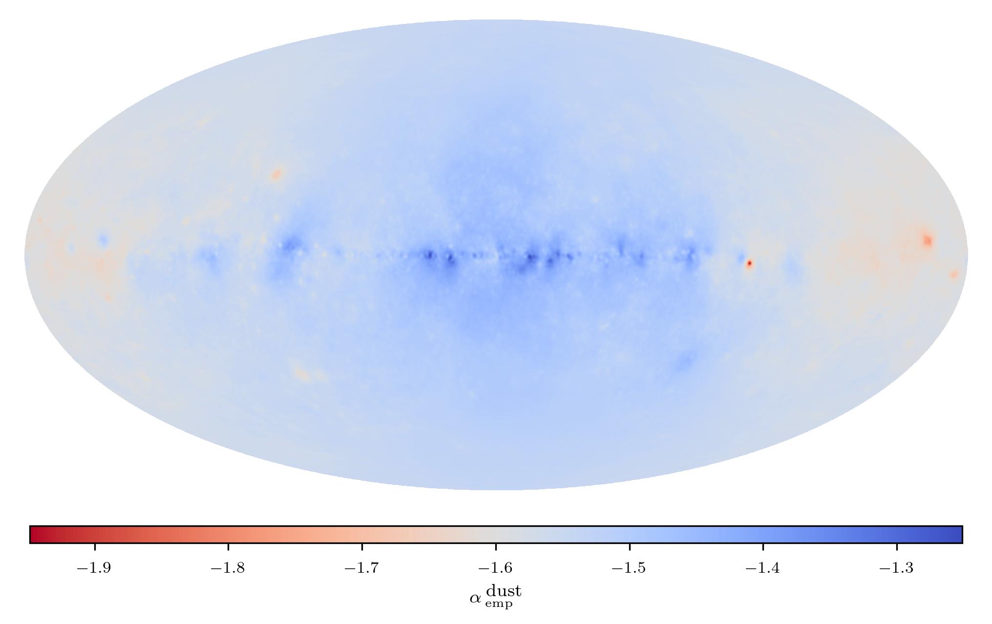
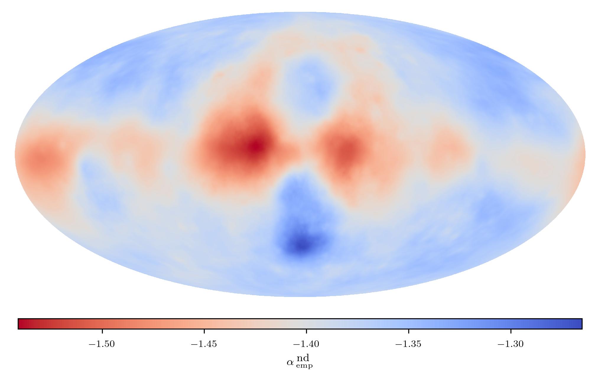
Figure 17: Maps of the M2 diffuse component empirical spectral index posterior means obtained by power-law fits to the diffuse emission component samples provided by the M2 reconstruction and subsequent averaging. Left: Map of the dust-template informed diffuse component pixel-wise spectral indices. Right: Map of the template-free diffuse component pixel-wise spectral indices.

Figure 17 shows empirical spectral index maps for the two diffuse components of M2. We obtained the values via power-law fits along the energy dimension of the diffuse maps and a subsequent averaging over posterior samples.

The left panel displays the spectral index map for the template-informed diffuse component. It shows a progressive spectral hardening toward the GC, from spectral indices of $-1.7$ in the Galactic anticenter to spectral indices of $-1.4$ near the GC ($-1.45$ when excluding the region occupied by the FBs). Only a few small-scale features are present. Among them are the region around extended objects already identified as deviating strongly from the dust template in Fig. 16. For those objects, a deviation from the spectral indices of the surrounding regions is expected, as they represent contamination in this map. More interestingly, the small-scale flat spectrum structures in the Galactic ridge already observed in Fig. 8, can now be seen with more clarity. They have no counterpart in the dust modification field (see Fig. 16), so we believe these structures to instead originate from a change in the local CR spectrum, making them indicative of hard spectrum CR injections in these locations.

The right panel of Fig. 17 displays the spectral index map for the template-free diffuse component $I^{\mathrm{\>nd}}$. It shows no small-scale structures, but has notable large-scale features. First, the spectral imprint of the FB emission is visible in blue, with spectral indices ranging from $-1.375$ to the highest observed value of $-1.26$. The bubbles are surrounded by a steep spectrum region symmetric around the GC, already observed in the spatio-spectral maps. It has spectral indices ranging from $-1.4$ down to the lowest observed value of $-1.54$. Additionally, in the Galactic plane but far from the GC lie areas of mildly steeper than average spectral indices, which roughly trace the dense ISM, but with a much smoother morphology. The remaining regions show slightly flatter than average spectra with spectral indices ranging from $-1.4$ to $-1.35$.

The properties of the two recovered diffuse emission components can also be studied by their CPSs as displayed in Fig. 7. The empirical APS of the template-informed component $I^{\mathrm{\>dust}}$ qualitatively follows the empirical APS of the M1 diffuse component. This is expected, as the M1 reconstruction is dominated by the dust-correlated emissions now taken up by $I^{\mathrm{\>dust}}$. However, it has a slightly steeper (posterior mean) power spectrum index of $-2.63$. The empirical APS of the M2 template-free diffuse component $I^{\mathrm{\>nd}}$ also shows a zigzag pattern induced by the bright Galactic disk, but this vanishes for angular modes above $|\ell|>10$. Before this threshold, the $I^{\mathrm{\>nd}}$ APS shows a steeper slope than the $I^{\mathrm{\>dust}}$ APS, while above it, they equalize in slope. The (posterior mean) APS index of $I^{\mathrm{\>nd}}$ is found to be $-2.45$. The APS of the dust modification field $\tau^{\mathrm{\>dust}}$ shows an overall flatter spectrum, with an empirical APS index of $-1.76$. This corresponds to a high degree of small-scale corrections to the emission template. Finally, the EPS indices for both components are very similar to each other ($-1.77$ for $I^{\mathrm{\>dust}}$ and $-1.70$ for $I^{\mathrm{\>nd}}$) and slightly lower than the value found for the M1 diffuse component ($-1.65$). The dust modification field shows a very flat EPS, with an empirical EPS index of $-0.12$. It has a peak at the harmonic log-energy scale $|q|=0.1$, pointing to a characteristic modulation scale of the $I^{\mathrm{\>dust}}$ energy spectra.

For an analysis of the PS results, we refer to the analysis done for M1 in Sect. 3.1, as the results do not differ qualitatively. Figure 29 shows the PS pixel brightness count distribution for M2. Similarly, the residual maps and histograms of the M2 reconstruction do not show qualitative differences to those of the M1 reconstruction. We therefore do not discuss them here, but include them in Appendix D. The M2 residuals have (to the stated precision) identical $\chi^{2}$ statistics as the M1 residuals.

3.3 Comparison of the imaging results

In this section we compare the results of imaging the gamma-ray sky with the two presented models and evaluate them for consistency.

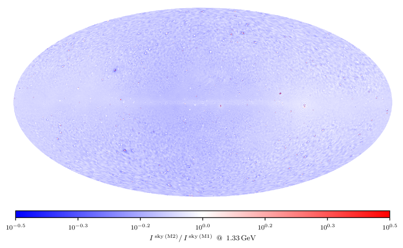
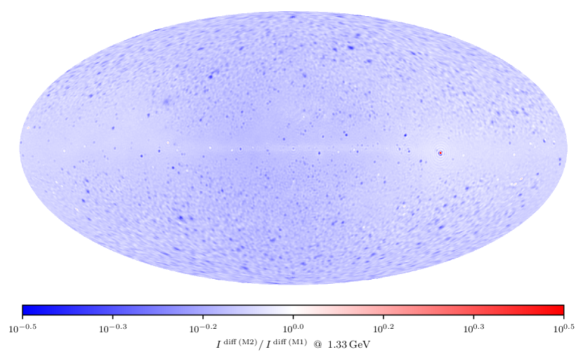
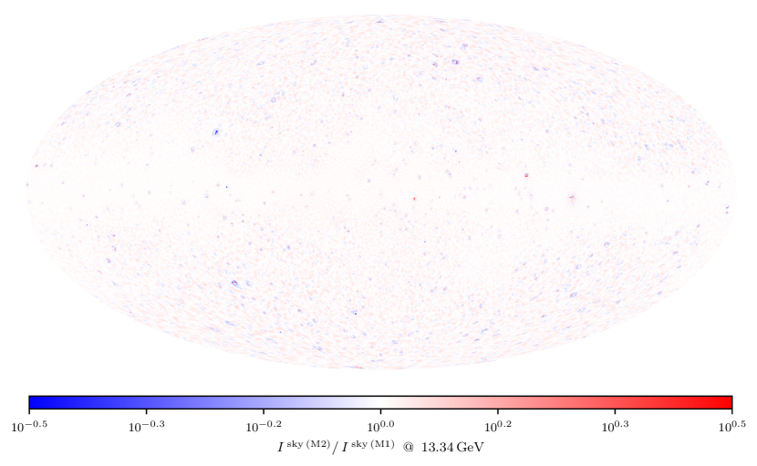
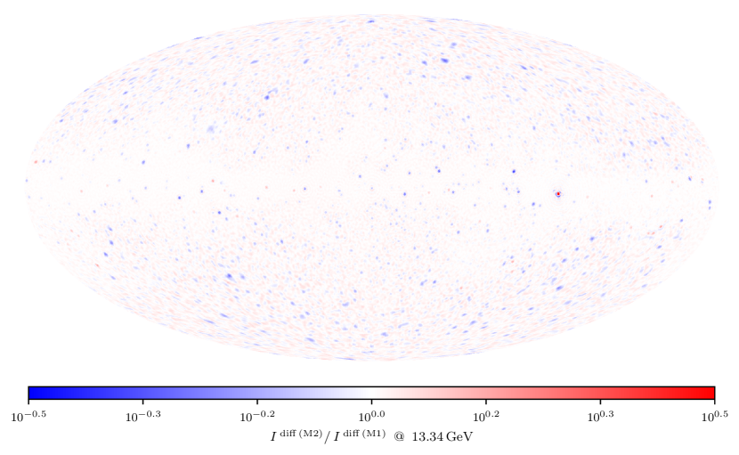
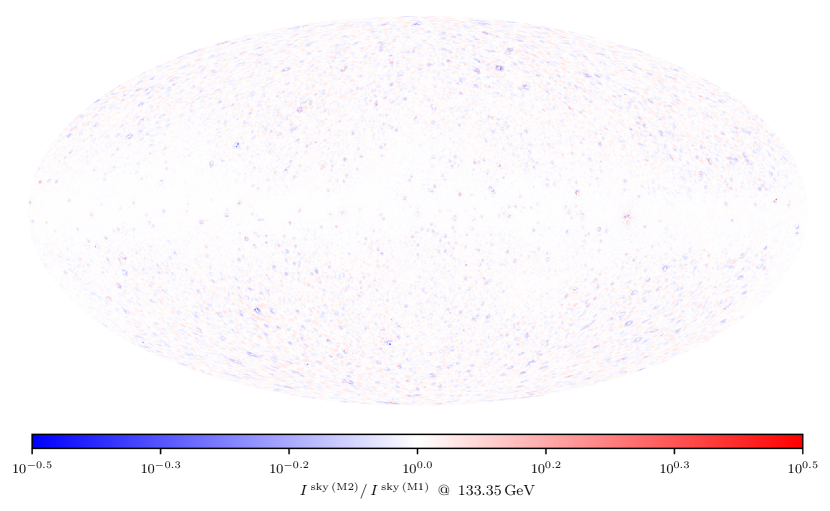
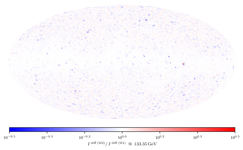
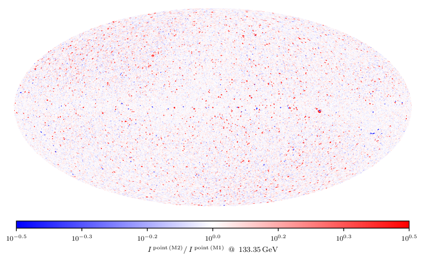
Figure 18: Ratio maps of the reconstructions based on M2 and M1. Left: Ratios of total sky flux values, $I^{\mathrm{\>(M2)}}/\,I^{\mathrm{\>(M1)}}$. Middle: Ratios of diffuse flux values, $I^{\mathrm{\>diffuse\>sum\,(M2)}}/\,I^{\mathrm{\>diffuse\,(M1)}}$. Right: Ratios of PS flux values, $I^{\mathrm{\>point\,(M2)}}/\,I^{\mathrm{\>point\,(M1)}}$. Energy bins: 1.00–1.77 GeV (top), 10.0–17.8 GeV (middle), and 100–178 GeV (bottom). The colorbars are logarithmic and shows equal fluxes as white.

Figure 18 shows the ratios of reconstructed total, diffuse and point-like fluxes in a low, medium, and high energy bin. We observe multiple systematic deviations between the reconstructions: First, the low energy ratio maps for the total sky and diffuse emission have a bluish tint, corresponding to a 20% reduction in isotropic emissions from M1 to M2. In the higher energy bins shown, this effect is not present. Second, there appears to be a shift of emission from the diffuse to the point-like emission component from M1 to M2, marked by corresponding blue spots in the diffuse and red pixels PS maps. This effect is visible in all energy bins shown. The only counter-example is in the location of Vela, where M2 found more PS flux than M1. Third, the PS maps show dim PSs found in one but not both reconstructions, visible as a background of slightly blue and red pixels.

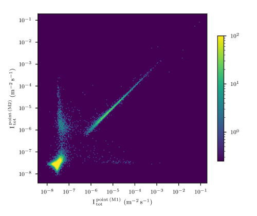
Figure 19: 2D histogram of M1 and M2 PS pixel brightness values $I^{\mathrm{\>point}}_{\mathrm{tot}}$. Both brightness values are binned on identical logarithmic scales. The histogram counts are shown with a logarithmic color scale. We note that emission from extended objects might be distributed into multiple PS pixels as we do not model them explicitly.

To analyze the repeatability of the PS detection further, Fig. 19 shows a scatter plot of the PS pixel brightness values found with the two models. This confirms that some PSs are switched-on in one reconstruction but remain switched-off in the other, where they sit at the high-brightness end of the deactivated source population. The figure shows very good agreement of PS brightness values for all switched-on source pixels over five orders of magnitude, with strong deviations only in a few very bright sources, which we discuss in the following section. The PSs additionally activated in M2 with respect to M1 contribute between ${10}^{-6}$ and ${10}^{-4}$ $\mathrm{m}^{-2}\,\mathrm{s}^{-1}$, changing their brightness by a factor of ${10}^{1.5}$ to ${10}^{3.5}$ in the process.

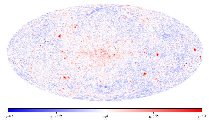
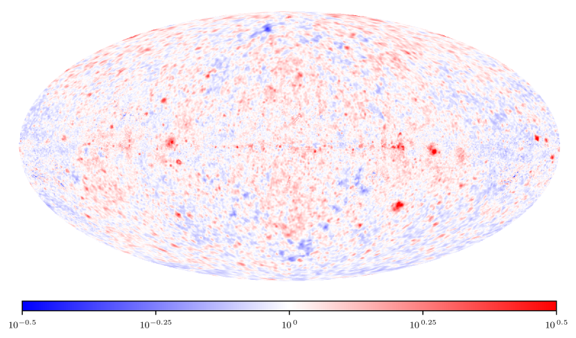
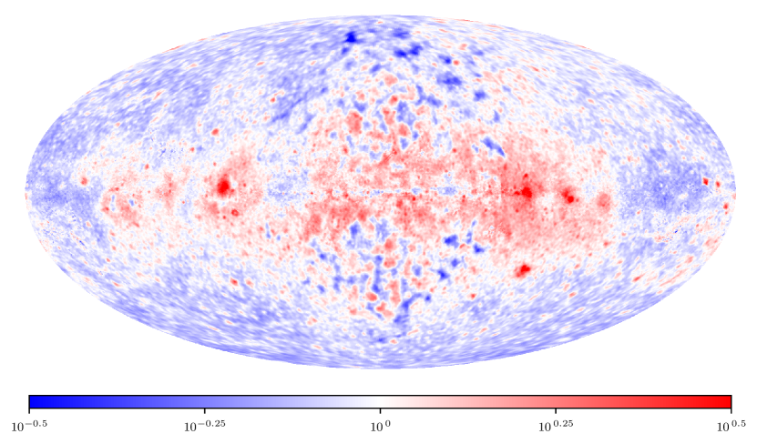
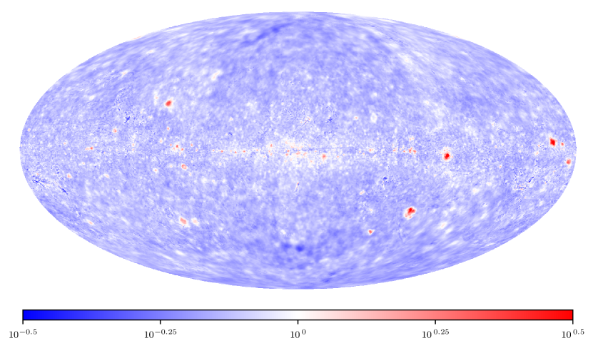
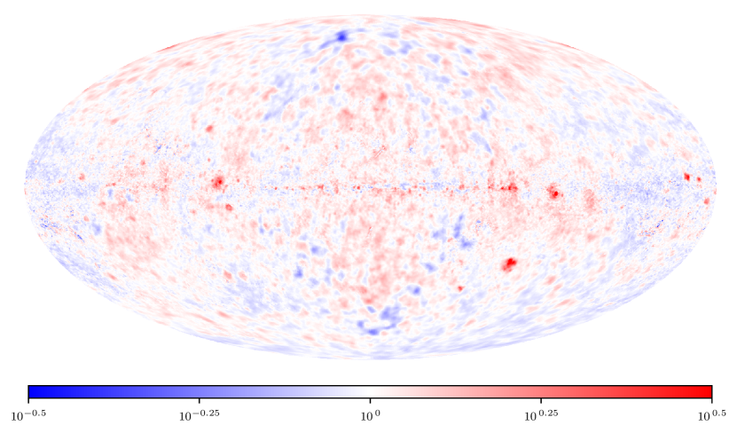
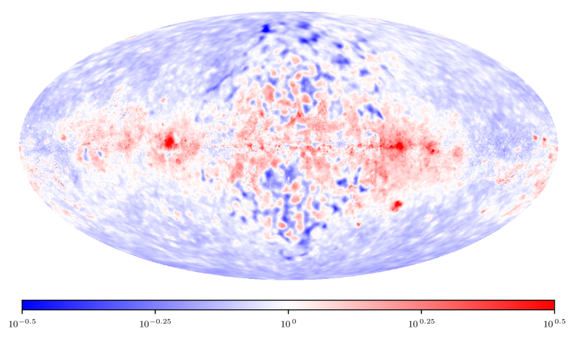
Figure 20: Ratio maps of our diffuse emission reconstructions and the Fermi diffuse and isotropic emission templates for the M1 (top row) and M2 (bottom row) reconstructions. The maps show our diffuse reconstructions divided by the values predicted by the Fermi templates in selected energy bins on a logarithmic color scale. Numbers larger than $10^{0}$ indicate we have reconstructed more flux than the template predicts, and vice versa. Energy bins: 0.56–1.00 GeV (left), 10.0–17.8 GeV (middle), and 178–316 GeV (right).

The observed shift of emission from the diffuse to the PS component in the M2 reconstruction also affects the agreement of this reconstruction with the Fermi diffuse emission template. Figure 20 shows flux ratio maps for our diffuse reconstructions and the Fermi template in selected energy bins. The flux ratio maps of M1 (top row) and M2 (bottom row) show that the reconstructions deviate from the Fermi templates in similar ways, as expected based on the comparison between the diffuse emission reconstructions above. However, there are some noteworthy differences: In the 0.56–1.00 GeV energy bin, we observe a flux under-prediction in the M2 map, corresponding to the uniform reduction in isotropic background found with M2 in this bin. In the 10.0–17.8 GeV energy bin, the M2 flux ratio map shows less small-scale structure than the M1 maps, related to the shift of flux from the diffuse emissions to the PS component. In the 178–316 GeV energy bin, the pattern of deviations from the Fermi templates is very similar in the two reconstructions.

4 Discussion

4.1 Quality of fit

As we claim to demonstrate data-driven imaging, we first want to discuss the achieved quality of fit. Judging from average reduced $\chi^{2}$ statistics, our reconstructions are able to explain the observed data well.

However, we do note clear signs of instrument response mismodeling. The residuals obtained with both sky models show PSF mismodeling artifacts (see Fig. 5 and 26). They indicate opposing PSF width errors for FRONT and BACK events, which we take as evidence against a systematic error in our PSF implementation as the source of this mismodeling. Artifacts of the mismodeling can also be found in the thermal dust template modification map of M2 (Fig. 16), where we observe an unphysical over-sharpening of the Galactic disk. Further, we observe evidence of EDF mismodeling (in the low-energy limit) in the energy spectra of bright PSs (Fig. 10). These IRF modeling errors are unfortunate, as they limit the fidelity of the acquired reconstructions, but they do not invalidate the demonstrated imaging approach.

The residual histograms reveal a slight bias of our models in the high energy limit through their ramped distribution (see the bottom-row panels of Fig. 4). This is a symptom of information density asymmetry between low, medium, and high energy data bins, driven by the vastly different photon counts in the different energy bins (see Fig. 1) and our spectral modeling of the sky flux, which assumes spectral continuity on logarithmic scales. This leads to information propagation between the energy bins, a central feature of spatio-spectral reconstructions. Both discussed limitations should be taken into consideration when deriving claims from the reconstructions presented.

Nevertheless, we achieved high-quality gamma-ray sky maps, as shown by the comparison with the Fermi diffuse emission template.

4.2 Agreement with the Fermi diffuse emission templates

Our analyses show a strong quantitative agreement of our diffuse emission reconstructions with the diffuse emission templates published by the Fermi Collaboration (see the discussions of Figs. 6,  20, and 28). The overall high Pearson correlation coefficient between our M1 reconstruction and the templates on log-log scale, $\left<\rho\right>=0.98$, and the geometric flux ratio mean and standard deviation of $1.01\pm 0.07$, together indicate close quantitative agreement of the maps.

In the low and medium energy regime, the deviations seem to be driven by extended emissions, which the Fermi diffuse emission templates exclude but which are included in our diffuse emission reconstruction. In the high energy limit, where observed photon numbers are low and correspondingly the data becomes less informative, we find the largest relative differences. Both our models produced similar deviation patterns from the templates in this limit, which suggests the existence of systematic errors in the creation of our maps and/or the templates. Relevant disagreements include the level of isotropic background flux, two large-scale smooth diffuse emission structures at low Galactic latitudes, and a pattern of medium-scale (5°) deviations in a large region surrounding the GC. We defer the analysis of these high-energy deviations to future work.

Overall, we observe a strong agreement of our reconstructions with the templates over many orders of magnitude of photon energy and flux density. We take this as a validation of our imaging approach and consider it an independent replication of the Fermi diffuse emission templates in the energy range of 0.5–100 GeV, up to the spatial and spectral resolution achieved in this work.

4.3 Template-informed imaging

The reconstructions based on the template-informed and template-free imaging models presented in this work broadly agree, indicating that no strong bias was introduced by the template. The differences found between the reconstruction demonstrate the benefits of template-informed imaging. In the M2 reconstructions, additional PSs were identified that had been absorbed by the diffuse component in the M1 reconstruction, as evidenced by the comparison of the diffuse reconstructions with the Fermi template (see the discussion of Fig. 20). This was driven by the inclusion of the template, which eliminated the need for the diffuse modification fields $\tau^{\mathrm{\>dust}}$ and $\tau^{\mathrm{\>nd}}$ to promote structures of this scale via their angular CPS models. Still, the template-informed component was able to incorporate the extended object emission, speaking to its flexibility with respect to the template and its data-drivenness.

The template-driven imaging produced separate reconstructions of dust-related and additional diffuse emissions, allowing us to study them individually. Judging from the log-log best-fit slopes between the obtained diffuse maps and the dust template (see Fig. 15), and the spectral index maps of the components (see Fig. 17), we find the separation into thermal dust template correlated and independent emissions was successful.

The dust correlated diffuse component shows a spectral hardening toward the GC, as reported by Gaggero et al. (2015), Acero et al. (2016), and Pothast et al. (2018). The spectral index shift from $-1.7$ to $-1.45$ is consistent with the values reported for the 2–228.65 GeV interval studied by Pothast et al. (2018), who find a spectral index hardening for the hadronic emission component from $-2.7$ at 33 kpc distance from the GC to $-2.45$ at 5 kpc distance from the GC. We want to point out that recently, Vecchiotti et al. (2022) hypothesized that the hardening observed in LAT studies may be an artifact of the LAT’s detection limits. Being a data-driven analysis, our work will certainly be susceptible to such data-inherent biases. If the hypothesis is found to be correct, updated instrument sensitivity models should allow this effect to be corrected.

We observe multiple sites with a localized hardening of the energy spectra in the inner Galaxy, both in the M1 diffuse spectral index maps (see Fig. 8), but more clearly in the M2 $I^{\mathrm{\>dust}}$ spectral index map (see the left panel of Fig. 17). These sites have an extension of a few degrees and as they have no counterpart in the dust modification map $\tau^{\mathrm{\>dust}}$ (see Fig. 16), we hypothesize that these structures show sites of CR injections into the ISM. Abdollahi et al. (2022a) test 4FGL sources for CR production via neutral pion decay emission. Their Fig. 6 shows a dense population of CR injecting sources in the region where we observe the spectral index aberrations. The local spectral hardening could also originate from PS contamination in the diffuse maps. However, on visual inspection of Fig. 14 and 24, we find no apparent PS contamination in the foci of the hypothesized outflow structures. Because of this and the extension of the observed structures, we disfavor the PS contamination hypothesis.

The a priori dust-independent diffuse emission map (see Fig. 13 and 14) shows a number of interesting features. We observe a constellation of “clumpy” structures surrounding the FBs and also finer clumpy structure within the FBs. These may all be caused by PS contamination, similar to the structures deleted from the diffuse reconstruction in M2, but both models robustly incorporated these emissions into the diffuse maps. Balaji et al. (2018) report finding only little small-scale structure in FBs, suggesting the clumpy structures observed by us are either contamination or outside the bubbles. As our focus is on presenting the employed methodology, we defer the detailed study of the obtained $I^{\mathrm{\>nd}}$ map to future publications.

Regarding the potential limitations of our template-informed reconstructions, we have two remarks: First, we note that the template-informed component $I^{\mathrm{\>dust}}$ reconstructed fluxes to one order of magnitude below the reconstructed isotropic background. The structures found in this limit have to be considered entirely template-driven, as even large relative changes to their flux density values would not significantly change the observed total flux in the corresponding pixels and so are not constrained by the likelihood.

Second, given that our template-informed model has a free second diffuse component that could in principle also absorb dust-connected emissions, we cannot guarantee that the “templating errors” of the thermal dust map with respect to the true dust-associated gamma-ray emission are entirely corrected by the modification field $\tau^{\mathrm{\>dust}}$, as assumed throughout this work. However, the extended emission structures included into the template-informed component demonstrated sufficient flexibility of the modification field to adopt even strong deviations from the dust template, supporting the presumption of nearly complete correction.

Perspectively, replacing templates with models of the gamma-ray production throughout the Galaxy and including data from other modalities currently used for the creation of the templates directly into the reconstruction holds the promise of producing globally consistent reconstructions of all involved physical quantities. Hutschenreuter et al. (2023) demonstrate this in a joint reconstruction of quantities related to the Galactic Faraday sky. Based on pulsar dispersion measure and distance data, extragalactic Faraday rotation measure data, and Planck free-free and H-$\alpha$ observations, they reconstruct the Galactic dispersion measure, line-of-sight parallel integrated magnetic field, and the emission measure-dispersion measure path length $\mathrm{L}_{\mathrm{DM}^{2}/\mathrm{EM}}$. Performing joint reconstructions of observed gamma-ray emissions, volumetric CR production density, transport, and interaction target densities in the Galaxy is the subject of ongoing research.

4.4 Point sources

In our presentation of reconstruction results, we show a number of PS emission analyses. For their reception, it should be noted that the PS model employed is reductionist in nature, not resolving individual PSs, but cumulative PS fluxes from the sky regions spanned by the pixels and has a fixed pixel brightness distribution prior. These modeling simplifications were made for the sake of implementational simplicity, but much more fine-grained PS analyses are available (see for example the source catalogs procured by the Fermi Collaboration). Also, our model is not able to resolve sub-detection-threshold PS properties, contrary to methods from the NPTF and 1pPDF families.

For the PS brightness distribution, we find a similar shape as the Fermi Collaboration (see the discussion of Fig. 9). Between ${10}^{-5}$ and $5\cdot{10}^{-4}$ $\mathrm{m}^{-2}\,\mathrm{s}^{-1}$, the source brightness count distributions of our reconstructions follow power laws of indices $-2.26$ (M1) and $-2.30$ (M2), deviating from the prior mean of $-2.5$. Previous works reported that the gamma-ray PS count distribution for high latitudes ($|\mathrm{b}|\leq 30\deg$) is better described by a (multiply) broken power law: Malyshev & Hogg (2011) find a spectral index of $n_{\mathrm{1}}=2.31$ below and $n_{\mathrm{2}}=1.54$ above $\mathrm{S}_{\mathrm{b}}=2.9\cdot 10^{-5}\>\mathrm{m}^{-2}\>\mathrm{s}^{-1}$ for the energy range of 1.0–300 GeV, while Zechlin et al. (2016) find a spectral index of $n_{\mathrm{1}}=3.1$ below and $n_{\mathrm{2}}=1.97$ above $\mathrm{S}_{\mathrm{b}}=2.1\cdot 10^{-4}\>\mathrm{m}^{-2}\>\mathrm{s}^{-1}$ for the energy range of 1.0–10 GeV. This suggests including broken power-law parametric source brightness distribution models in future analyses to elucidate to which degree the brightness distributions observed by us are data- and prior-driven. However, given that the inferred PS brightness distribution strongly deviates from the prior distribution (single power law with low brightness cutoff), we assume it to be mostly data-driven for the activated source pixels.

The analysis of PS consistency between our two models (Fig. 19) shows that most PSs are reconstructed consistently, but this breaks down in the high-flux limit. We believe this is an effect of extended sources, specifically close pulsar wind nebulae, which produce both PS flux via their central pulsar and extended emission from the jet and surrounding medium. These objects are not well representable by our emission component models, making different splits of the flux equally well-fitting. Because of this, different combinations of PS and diffuse emission are reconstructed, depending on the general state of the emission components (for example, learned angular power spectra). An explicit modeling of extended emission objects could alleviate this problem and lead to more stable bright PS reconstructions. However, for a priori unknown extended structures, this will still fail. The automated treatment of extended objects found superimposed on the sky in a Bayesian framework is ongoing research.

4.5 Caveats for studies of the 1–5 GeV energy range

As laid out in the introduction, the GCE is subject of long-standing interest in the gamma-ray astronomy community. Its emission lies mostly in the 1–5 GeV band, making this energy range particularly relevant for down-stream analyses of the maps we provide.

In Sect. 3.1, we discuss that we have reduced data-drivenness in the 0.56–1.0 GeV and 1.0–1.77 GeV energy bins, because the strong EDF of the LAT at energies below 1 GeV prevents us from using the data bin corresponding to the lowest reconstructed energy in our likelihood. This makes the reconstructions in the lowest two energy bins especially vulnerable to IRF mismodeling, and warrants a discussion of the dependability of the reconstructions in the corresponding energy range.

For the PS spectra reconstructed based on M1 (Fig. 10), we observe spectral artifacts for bright PSs in the lowest two energy bins, leading us to recommend excluding them from analyses. For the M1 diffuse emission reconstruction, comparison with the Fermi diffuse emission templates shows good agreement in these low energy bins (Fig. 6), suggesting they are not affected as strongly by spectral artifacts. For the M2 diffuse emission reconstruction, a difference in isotropic background flux with respect to the Fermi templates (see Fig. 28) and the M1 diffuse reconstruction (see Fig. 18) is present in the lowest energy bin, which could be caused by IRF mismodeling in conjunction with the described “under-informedness.” We therefore recommend caution when analyzing the two lowest energy bins of the M2 diffuse reconstructions.

4.6 Cosmic ray background contamination

Our reconstructions are based on the P8R3_SOURCE event class, while analyses of the diffuse emissions usually use more restrictive event classes (P8R3_ULTRACLEAN and P8R3_ULTRACLEANVETO). This means the data set we use has a higher level of CR contamination than in comparable analyses, which might bias our reconstruction to find more isotropic gamma-ray background than truly exists. However, the higher photon count in the P8R3_SOURCE event class compared to the more commonly used restrictive event classes also makes our analysis more sensitive to faint emission sources, which we optimized for in selecting the event class. Different trade-offs between faint emission sensitivity and CR background susceptibility can be explored by repeating the reconstructions with the other event classes and cuts provided by the Fermi Collaboration.

4.7 Potential improvements

As already mentioned above, the presented imaging models can be improved in a number of ways.

First, we demonstrate the template-informed imaging using only one template for simplicity. However, generally, the use of additional emission templates leads to improvements in reconstruction fidelity and enables further separation of the emission components, as demonstrated by the full body of work on template-based analyses. To facilitate searches for DMA or decay, corresponding emission models can be added.

Second, improvements to the modeling of PS and extended emissions would lead to higher fidelity reconstructions of all emission components. For the former, techniques such as iterative charted refinement (ICR; Edenhofer et al. 2022) hold promise. Iterative charted refinement can facilitate the construction of $\tau^{\mathrm{\>c}}$ fields with locally increased resolution and allows local deviations in the correlation structure, which are necessary for a correct modeling of extended object emission.

Third, we did not include a separate component for the isotropic diffuse background, which forced our diffuse emission component to absorb it. In the template-informed imaging run, this limited the dynamic range of the template-free component $I^{\mathrm{\>nd}}$. Including a separate isotropic emission component (low parameter count model) would allow the non-isotropic diffuse emissions components to learn more specific correlation structures for their emissions.

Fourth, improvements to the accuracy of the instrument response model would increase the fidelity of the obtained results, as is true for all similar analysis methods.

Fifth, the studied energy range, as well as the spatial and spectral resolution are currently limited by computational constraints, specifically, the computational efficiency and scalability of the numerical PSF operator implementation. Improvements in this regard would enable higher resolution reconstructions and make an expansion of the reconstructed energy range to lower energy bins feasible, where the PSF becomes increasingly wide. This would allow a more robust study of the 1–5 GeV energy range and the GCE than the current reconstruction affords.

Further potential for improvement lies in the inference methodology itself. Frank et al. (2021) recently published Geometric Variational Inference, a generalization of MGVI, which improves the fidelity of the estimated posterior samples with respect to MGVI for non-Gaussian posterior distributions. At the cost of additional computational resources, such methods can increase the fidelity of the reconstructed sky maps. We leave the realization of this to future work.

5 Conclusions

We present a template-independent spatio-spectral imaging approach for the gamma-ray sky, based on a Bayesian framework. We demonstrate its capabilities on data produced by the Fermi LAT, showing a template-free and a template-informed reconstruction of the gamma-ray sky. In the latter case, we include the Planck 545 GHz thermal dust emission map as a tracer of sites of interaction between CR protons and ISM protons in our sky model. The reconstructions are highly data-driven, giving them high sensitivity to unexpected emissions by construction. This is achieved through the use of Gaussian processes for modeling the emission components constituting the gamma-ray sky, and in the case of the template-informed component, for modeling deviations of the respective emission component from the template. We used an instrument response model based on the in-flight-calibrated IRFs published by the Fermi Collaboration and fully modeled the Poissonian statistics of the emissions. With our instrument and sky models, we achieve an overall good quality of fit, but also observe evidence of instrument response mismodeling.

The imaging approach we present extends existing concepts for template-based imaging to the fully data-driven limit while still relying on classical hierarchical generative models for the inference. This way, we retain the direct interpretability of our model parameters, in contrast to DL-based methods. Based on hierarchical generative models, characteristic spatial and spectral correlation scales of the individual emission components are detected automatically and used to image them more accurately. The work lays out a recipe for more complex sky models based on the presented methods, allowing the inclusion of further templates, emission components, and more complex modeling of the existing subcomponents.

We have presented and analyzed the results of our reconstructions, which include individual spatio-spectral maps for all assumed emission components, summary statistics that are part of their generative models (such as spatial and spectral power spectra), and an uncertainty quantification of any resulting quantities in terms of self-consistent posterior samples. Comparing our diffuse reconstructions with the sum of the Fermi diffuse emission templates gll_iem_v07 and iso_P8R3_SOURCE_V3_v1, we find strong quantitative agreement, with pixel-wise flux ratios in the range $0.5$–$2$, a geometric mean flux ratio of $1.01$, and an average Pearson correlation between the two maps on log-log scale of $\rho=0.98$. Comparing our diffuse reconstructions with the Planck 545 GHz thermal dust emission map, we find a strong linear scaling on log-log scale for the dust-informed emission component ($\alpha=0.94$) and a weak linear scaling on log-log scale for the second diffuse component of the template-informed reconstruction ($\alpha=0.28$), indicating a successful flux separation in the template-informed model. We show and discuss spectral index maps of reconstructed emission components, where we find a spectral hardening of hadronic emissions from -1.7 in the Galactic anticenter to -1.4 in the GC, consistent with literature values. We analyzed the retrieved pixel-wise PS fluxes and find a population of activated PS flux pixels between ${10}^{-6}$ and ${10}^{-3}$ $\mathrm{m}^{-2}\mathrm{s}^{-1}$, with luminosity function power-law indices of $-2.26$ and $-2.30$ between ${10}^{-5}$ and $5\cdot{10}^{-5}$ $\mathrm{m}^{-2}\mathrm{s}^{-1}$ for our two reconstructions, respectively. For these PS fluxes, we find energy spectral indices in the range $\left[-2.15,-0.35\right]$. For the diffuse emission components, we find empirical angular power spectra with spectral indices between $-2.63$ and $-2.48$ and empirical EPSs with spectral indices between $-1.77$ and $-1.65$.

We believe the presented imaging approach is a valuable addition to existing analysis methods and will help such methods reach their full potential.

Appendix A Generative models of the $\gamma$-ray sky

A.1 General remarks

For Bayesian inference, it is convenient to express the sky components in terms of generative models. A generative model is a description of a stochastic process that is able to generate random realizations following a desired target statistic. Following Knollmüller & Enßlin (2018), we constructed our generative models to take a vector of uncorrelated random variables $\xi=(\xi_{1},\xi_{2},\ldots)$, here assumed to be standard normal distributed, with

$$\mathcal{P}(\xi)=\prod_{j}\mathcal{\mathcal{{N}}}(\xi_{j}|0,1)=\prod_{j}\left[\exp(-\xi_{j}^{2}/2)/\sqrt{2\pi}\right],$$ (16)

and to apply a transformation $T$ to it to turn $\xi$ into a potential signal vector $s=T(\xi)$ including all quantities of interest that are reconstructed from the observations. The transformation $T$ has to be chosen such that the required signal statistics $\mathcal{P}(s)$ result from the transformed Gaussian statistics $\mathcal{P}(\xi)$ via

$$\left.\mathcal{P}(s)\right|_{s=T(\xi)}=\mathcal{P}(\xi)\left\|\frac{\partial T(\xi)}{\partial\xi}\right\|^{-1}.$$ (17)

Such a transformation exists for any hierarchical probabilistic model over continuous quantities and can be accessed via inverse transform sampling (Knollmüller & Enßlin 2018).

The latent parameters $\xi$ are our effective parameterization of the model and are to be learned from the data. The physical signal $s$ corresponding to a recovered $\xi$ can always be obtained via $s=T(\xi)$.

For the models presented here, we make heavy use of the generative correlated field model introduced by Arras et al. (2021, Sect. 3.4) and Arras et al. (2022, Methods), summarized in Frank et al. (2021, Appendix B). It allows us to translate prior knowledge on the spatial and spectral correlation functions of modeled quantities into appropriate transformation functions $T$.

To this end, we represent the spatial and spectral correlation functions of the modification fields $\tau^{\mathrm{\>c}}$ via power spectra in the corresponding harmonic spaces, the SH space with coordinates $k=(\ell,m)$ for the spatial dimensions and the 1D Fourier space with coordinate $q$ for the log-energy dimension. The harmonic representation of $\tau^{\mathrm{\>c}}$ in this space is defined via

$$\tau^{\mathrm{\>c}}(x,y)=\sum_{\ell m}Y_{\ell m}(x)\,\int\frac{\mathrm{d}q}{2\pi}\,\mathrm{e}^{-iqy}\,\hat{\tau}^{\mathrm{\>c}}(k,q),$$ (18)

where $Y$ denotes the SH functions. Thanks to the assumed separability of the correlation functions in spatial and spectral directions, the corresponding power spectra are separable as well. Thus, for components c and c’, we have

$$\langle\hat{\tau}^{\mathrm{\>c}}(k,q)\;\hat{\tau}^{\mathrm{\>*\,c^{\prime}}}(k^{\prime},q^{\prime})\rangle_{(\tau)}=2\pi\,\delta_{cc^{\prime}}\delta_{\ell\ell^{\prime}}\delta_{mm^{\prime}}\delta(q-q^{\prime})\,\hat{C}^{\mathrm{\>c}}(\ell)\,\hat{D}^{\mathrm{\>c}}(q).$$ (19)

Here, $\hat{C}^{\mathrm{\>c}}(\ell)$ is the spatial APS of $\tau^{\mathrm{\>c}}$. It is assumed to be isotropic and therefore does not depend on $m$. $\hat{D}^{\mathrm{\>c}}(q)$ is the corresponding log-energy Fourier power spectrum of $\tau^{\mathrm{\>c}}$. $\hat{\tau}^{\mathrm{\>*}}$ denotes the complex conjugate of $\hat{\tau}$. The $2\pi$ in Eq. 19 results from the adopted Fourier convention for the log-energy space,

$$f(q) = \int\mathrm{d}y\,\exp(iqy)\,f(y)$$ (20)

$$f(y) = \frac{1}{2\pi}\int\mathrm{d}q\,\exp(-iqy)\,f(q).$$ (21)

The correlated field model generates harmonic space samples of the field $\tau^{\mathrm{\>c}}$ by drawing independent unit Gaussian random numbers $\xi^{\mathrm{\>c}}(k,q)$ and multiplying these point-wise with the amplitude spectra according to

$$\hat{\tau}^{\mathrm{\>c}}(k,q)=\sqrt{\hat{C}^{\mathrm{\>c}}(\ell)\hat{D}^{\mathrm{\>c}}(q)}\;\xi^{\mathrm{\>c}}(k,q)=:A^{\mathrm{\>c}}_{\mathrm{\tau}}(k,q)\;\xi^{\mathrm{\>c}}(k,q).$$ (22)

Realizations of $\tau^{\mathrm{\>c}}(x,y)$ can then be obtained via the inverse harmonic transforms to the original $(x,y)$ coordinates as given above. By construction, these exhibit the requested correlations in spatial and log-energy dimension.

Since a priori we do not know the exact power and corresponding amplitude spectra, the correlated field model represents them through further generative processes. By specifying their prior statistics, we encoded our prior knowledge on the spatial and spectral correlation functions. We show the construction here for the angular power spectra $\hat{C}(\ell)$, but the $\hat{D}(q)$ are constructed analogously. The CPSs are modeled similar to the gamma-ray emission models, as modified power laws in the harmonic modes,

$$\hat{C}(\ell)={|\ell|}^{\,\beta}\cdot e^{\kappa\,\left(\ln|\ell|\right)}.$$ (23)

Here, $\beta$ specifies the power-law index and $\kappa$ models the deviations from a pure power law in $|\ell|$ on log-log scale. We placed a Gaussian prior on the power-law index $\beta$ with prior mean $\mu_{\beta}$ and prior standard deviation $\sigma_{\beta}$. The deviations, $\kappa$, were modeled via an integrated Wiener process (see Eqs. 20 to 24 of Arras et al. 2021 for a precise definition). This allows us to specify separate priors on the deviation amplitude on log-log scale and on the spectral roughness.

In the PS spectrum model $f_{\mathrm{spec}}$, the energy spectrum fluctuations $\epsilon_{\mathrm{ij}}$ were built using the same integrated Wiener process formulation as we use for $\kappa$.

A.2 Prior parameters of the sky models

Figure 21: Structure of the main generative hierarchical Bayesian models used in the inference. The initial, abstract, and Gaussian-distributed degrees of freedom, $\xi$, are mostly left out for the sake of clarity. The dashed component indicates a set of instances of the Gaussian correlated field model introduced by Arras et al. (2021, Sect. 3.4). Left: Template-free model M1 with diffuse and point-like fluxes $I^{\mathrm{\>diff}}$ and $I^{\mathrm{\>point}}$. Right: Template-informed model M2 with the additional template-informed diffuse flux component $I^{\mathrm{\>dust}}$. $I^{\mathrm{\>nd}}$ is identical in construction to $I^{\mathrm{\>diff}}$, but has different prior parameter values. $I^{\mathrm{\>point}}_{\mathrm{ij}}$ is defined identically in both models.

Parameter	Value
$\alpha_{\text{I}\Gamma}$	$1.5$
$\beta_{\text{I}\Gamma}$	$5\cdot{10}^{-4}$ $(\mathrm{m}^{2}\,\mathrm{s}\,\mathrm{sr})^{-1}$
$\epsilon_{\mathrm{flex}}$	$\mathfrak{m}=0.5,\;\mathfrak{s}=0.25$
$\epsilon_{\mathrm{asp}}$	$\mathfrak{m}=0.05,\;\mathfrak{s}=0.05$
$\mu_{\mathrm{ap}}$	$-1.25$
$\sigma_{\mathrm{ap}}$	$0.3$

Table 1: Prior parameters of the PS emission model in M1 and M2.

Parameter	Value
$I^{\mathrm{\>diff}}\;$ (M1)
$I^{\mathrm{\>diff}}_{0}$	${10}^{-2}$ $\mathrm{m}^{-2}\,\mathrm{s}^{-1}\,\mathrm{sr}^{-1}$
$\alpha^{\mathrm{\>diff}}$	$-1.466$
$\hat{C}_{\beta}$	$\mu_{\beta}=-3.0,\;\sigma_{\beta}=0.25$
$\tau^{\mathrm{\>diff}}_{\mathrm{fluct\,x}}$	$\mathfrak{m}=0.75,\;\mathfrak{s}=0.187$
$\hat{D}_{\gamma}$	$\mu_{\gamma}=-3.5,\;\sigma_{\gamma}=0.25$
$\tau^{\mathrm{\>diff}}_{\mathrm{fluct\,y}}$	$\mathfrak{m}=0.1,\;\mathfrak{s}=0.05$
$I^{\mathrm{\>nd}}\;$ (M2)
$I^{\mathrm{\>nd}}_{0}$	$I^{\mathrm{\>diff}}_{0}/2$
$\alpha^{\mathrm{\>nd}}$	$-1.25$
$\hat{C}_{\beta}$	$\mu_{\beta}=-3.0,\;\sigma_{\beta}=0.25$
$\tau^{\mathrm{\>nd}}_{\mathrm{fluct\,x}}$	$\mathfrak{m}=0.75,\;\mathfrak{s}=0.187$
$\hat{D}_{\gamma}$	$\mu_{\gamma}=-3.5,\;\sigma_{\gamma}=0.25$
$\tau^{\mathrm{\>nd}}_{\mathrm{fluct\,y}}$	$\mathfrak{m}=0.1,\;\mathfrak{s}=0.05$
$I^{\mathrm{\>dust}}\;$ (M2)
$I^{\mathrm{\>dust}}_{0}$	$I^{\mathrm{\>diff}}_{0}/2$
$\alpha^{\mathrm{\>dust}}$	$-1.65$
$\hat{C}_{\beta}$	$\mu_{\beta}=-3.5,\;\sigma_{\beta}=0.25$
$\tau^{\mathrm{\>dust}}_{\mathrm{fluct\,x}}$	$\mathfrak{m}=0.25,\;\mathfrak{s}=0.125$
$\hat{D}_{\gamma}$	$\mu_{\gamma}=-3.0,\;\sigma_{\gamma}=0.25$
$\tau^{\mathrm{\>dust}}_{\mathrm{fluct\,y}}$	$\mathfrak{m}=0.1,\;\mathfrak{s}=0.025$
Common parameters
$\mathrm{Std}[\langle\tau^{\mathrm{\>c}}\rangle]$	$\mathfrak{m}=0.5,\;\mathfrak{s}=0.05$
$\hat{C}\kappa_{\mathrm{flex}}$, $\hat{D}\kappa_{\mathrm{flex}}$	$\mathfrak{m}=0.1,\;\mathfrak{s}=0.1$
$\hat{C}\kappa_{\mathrm{asp}}$, $\hat{D}\kappa_{\mathrm{asp}}$	$\mathfrak{m}=0.1,\;\mathfrak{s}=0.05$

Table 2: Prior parameters of the diffuse emission components of M1 and M2.

Figure 21 shows the hierarchical structure of the employed sky models M1 and M2, while Table 1 and 2 provide the corresponding prior parameters. In the following, we give additional background information to help with their interpretation.

Single parameter values indicate the parameter is a constant in the model and cannot be modified during reconstruction. Parameter values typeset as tuples indicate the model parameter is assumed to be either normal or log-normal distributed a priori. If $\mu$ and $\sigma$ values are given, we chose a normal distribution with mean $\mu$ and standard deviation $\sigma$ as the parameter prior. If $\mathfrak{m}$ and $\mathfrak{s}$ values are given, a log-normal prior distribution in accordance with Arras et al. (2021, Eq. 16 and Eq. 17) is assumed.

A practical demonstration of how the correlated field parameters affect the generated field samples can be found at the NIFTy documentation page and the source code of this demonstration is published at the NIFTy code repository. We used the “add_fluctuations” call of the correlated field model. The model parameters for the APS and EPS $\beta$ and $\gamma$ correspond to its “loglogavgslope” parameter, while $\kappa_{\mathrm{flex}}$ and $\kappa_{\mathrm{asp}}$ correspond to the “flexibility” and “asperity” parameters. The correlated field standard deviation in the energy dimension $\tau^{\mathrm{\>c}}_{\mathrm{fluct\,y}}$ and the spatial dimension $\tau^{\mathrm{\>c}}_{\mathrm{fluct\,x}}$ is set via the fluctuations parameter in the add_fluctuations function. The a priori standard deviation of the offset from zero of the $\tau$ fields is parameterized by the $\textrm{Std}[\langle\tau^{\mathrm{\>c}}\rangle]$ parameter, which corresponds to the “offset_std” parameter of the “CorrelatedFieldMaker.”

Appendix B Instrument response model implementation

B.1 Overview

The Fermi Collaboration provides high-quality IRF models for the LAT, obtained via Monte Carlo simulations of the instrument in action and validated with online measurements.

B.2 Point spread function

The PSF probabilistically describes how the Fermi LAT misclassifies the origin direction of recorded gamma-ray photons. Of the Fermi LAT IRF components, the convolution with the PSF was the hardest to model numerically. Usually, convolutions can be efficiently performed by multiplication in a corresponding harmonic space. However, the Fermi LAT PSF is not band-limited in SH space, which makes it unfit for this approach. We therefore chose to numerically represent the PSF convolution operation with a sparse matrix application. For this, we calculate the contribution of each pixel to every other pixel under convolution with the PSF. To quantify this contribution, the PSF needed to be integrated over the receiving pixel areas, once for each source pixel. We perform this integration using Monte Carlo methods, specifically direct sampling from the angular deviation distribution described by the PSF. The drawn samples were binned into the respective sky pixels and the count normalized by the total sample count. This integration method yields the highest accuracy in the pixels receiving the most flux under the PSF convolution, while still capturing the broad-tailed nature of the PSF. The PSF application matrix was sparsified by discarding entries with contributions below $10^{-7}$ times the maximum contribution.

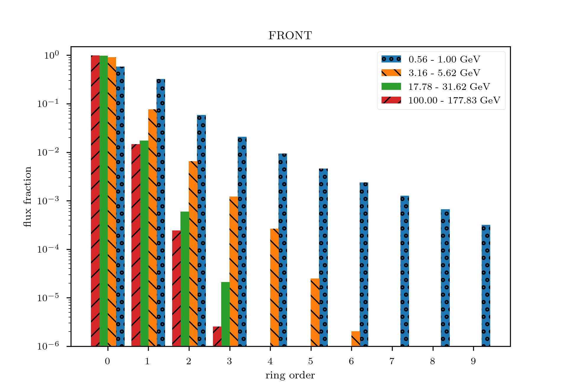
Figure 22: Flux fractions distributed into concentric rings around the origin pixels by the PSF of the $\cos(\theta)\in\left(0.9,\,1.0\right]$ incidence direction bin for FRONT and BACK events and selected energy bins. Ring order 0 corresponds to the origin pixel itself, ring order 1 to the eight pixels surrounding it, and so forth. Table 3 provides the average $\delta\theta$ values of the pixels in the rings. Flux fractions are shown on a logarithmic scale from ${10}^{-6}$ to $1.0$.

To evaluate how the PSF modeling interacts with the spatial discretization, we analyzed how the PSF matrices distribute flux into concentric rings of pixels around selected source pixels. For this, we calculated how much flux is retained in the source pixel itself, in the eight pixels surrounding it, in the 26 pixels surrounding these, and further on. We call these groups of pixels rings of order zero, one, two, and higher. Figure 22 shows the flux fractions distributed into the respective rings for FRONT and BACK events in selected energy bins. The figure shows the expected patterns. With increasing bin energy, the instrument point spread becomes weaker. This is captured by our PSF model matrices, which leave increasing amounts of flux in the source pixel for increasing energy (see the ring order zero bars in both panels). For the two highest energy bins shown, only an original flux fraction on the order of one percent is distributed away from the source pixel for FRONT events. For BACK events, in the same energy bins on the order of 10% of the flux is redistributed by the PSF model matrix.

Ring order	0	1	2	3	4	5	6	7	8	9
Average $\delta\theta$	$0.0^{\circ}$	$0.57^{\circ}$	$1.09^{\circ}$	$1.62^{\circ}$	$2.18^{\circ}$	$2.73^{\circ}$	$3.29^{\circ}$	$3.87^{\circ}$	$4.45^{\circ}$	$5.07^{\circ}$

Table 3: Average $\delta\theta$ values of the pixels belonging to the rings presented in Fig. 22.

Table 3 provides the average $\delta\theta$ values of the pixels belonging to the rings. The $\delta\theta$ values of the pixels are calculated by finding the angle between the vectors pointing to the center of the source pixel and the center of the receiving pixel from the center of the sphere.

B.3 Energy dispersion function

The EDF probabilistically describes how the Fermi LAT misclassifies the energy of recorded gamma-ray photons. Similar to the PSF modeling, the effect of the convolution with the EDF of the LAT was modeled numerically using a matrix. Since the EDF describes how specific photon energies are misclassified, a double integral needs to be calculated to estimate the contributions of individual energy bins toward each other: First, integration of the true photon energy over the source energy bin and second, integration of the recorded photon energy over the target energy bin. Since the photon flux density is not constant within the energy bins, in the first integral a weighting factor has to be considered. We estimated this weighting factor from a power-law fit to the raw photon counts.

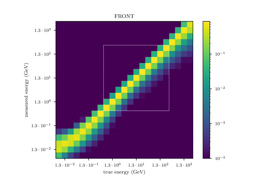
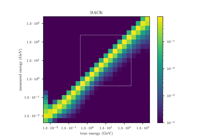
Figure 23: Energy dispersion matrices of the $\cos(\theta)\in\left(0.9,\,1.0\right]$ incidence direction bin for FRONT and BACK events. True and measured energies are shown on logarithmic scales. The figure shows how flux from each true energy is distributed to the observed energy bins by the measurement process and has a logarithmic color scale. The white rectangle marks the EDF matrix entries used in this work, which were selected based on the studied energy range.

Figure 23 shows the distribution of flux between energy bins prescribed by the EDF matrix employed in our model. The Fermi Collaboration published a similar figure entitled “Detector Response Matrix” on the website describing the usage of the Pass 8 energy dispersion characterization.

B.4 Exposure maps

Exposure maps were calculated based on the spacecraft files provided with the event tables by the Fermi Collaboration and take into account the data cuts we describe in Sect. 2.5. To get total exposure values for all data bins, first we calculated exposure maps for each 30 s time slice specified in the spacecraft files, and afterward took their sum along the temporal axis as the total exposure. To calculate the exposure values for a time slice, we first calculated a binary “data bin reachability mask” based on the instrument pointing, the data bins’ incidence direction window, the Earth albedo cut for the corresponding time frame, and the zenith cut. Second, for all data bins included by the reachability mask we set the exposure value to the active observation time of the LAT in the corresponding time slice (as specified by the spacecraft files). All data bins “unreachable” during the time slice were set to have 0 s of exposure. The resulting time slice exposure maps were added up for all included mission weeks to form the total exposure maps.

B.5 Effective area

The effective area of the instrument is provided by the Fermi Collaboration at much higher resolution than the other IRFs. For the sake of simplicity, we averaged the values over the coarser incidence direction and energy bins employed in the PSF parameter table and used these averages in our instrument response model.

Appendix C Color coding of multi-energy sky maps

Throughout this article, we show several sky maps in which energy information is color-coded. In these maps, we simulate how a non-color-blind human would perceive the visualized gamma-ray fluxes if the photon energies were shifted into the visible light spectrum range. This presentation is optimized for a natural perception of spectral variations.

To obtain high spectral contrast and a natural appearance of the resulting maps, we performed the following preprocessing steps before mapping to perceived colors: First, we multiplied the spatio-spectral flux map with an energy-dependent scaling function to compensate for flux density decrease toward high energies (see the middle panel of Fig. 2). Second, we transformed the values to a logarithmic scale. Third, we clipped the logarithmic values to a predefined range (corresponding to the visualized dynamic range) and rescaled them to lie in the $[0,1]$ interval. Fourth, we applied a gamma correction with exponent $1.675$.

For the perceived color mapping, we then mapped the reconstructed gamma-ray energies to visible light wavelengths (log-linearly) and for each pixel used the CIE 1931 model of human color perception to determine the chromaticity and luminosity a human would perceive if looking into a light source of the corresponding visible light spectrum. The corresponding perceived color values of the pixels were then embedded in the sRGB color space (International Electrotechnical Commission et al. 1999) for rendering.

As a last step, we applied a color saturation correction. For this, we calculated the gray value $L$ of each image pixel from the sRGB values,

$$L=0.2989r\>+\>0.5870g\>+\>0.1140b,$$ (24)

and the color difference of each pixel from its gray value,

$$\left(\delta r,\,\delta g,\,\delta b\right)=\left(r-L,\,g-L,\,b-L\right).$$ (25)

The final sRGB pixel values were then set to the color-saturation-enhanced

$$\left(r^{\prime},\,g^{\prime},\,b^{\prime}\right)\,=\,2.2\cdot\left(\delta r,\,\delta g,\,\delta b\right)\,+L.$$ (26)

The bottom panel of Fig. 2 shows the resulting mapping of mono-energetic gamma-ray fluxes (after energy-dependent scaling) to sRGB values. Figure 30 shows selected M2 reconstruction results rendered without application of the color saturation enhancement.

Appendix D Additional plots

This section contains additional figures that were excluded from the main text to save space, but that we nevertheless want to include for completeness.

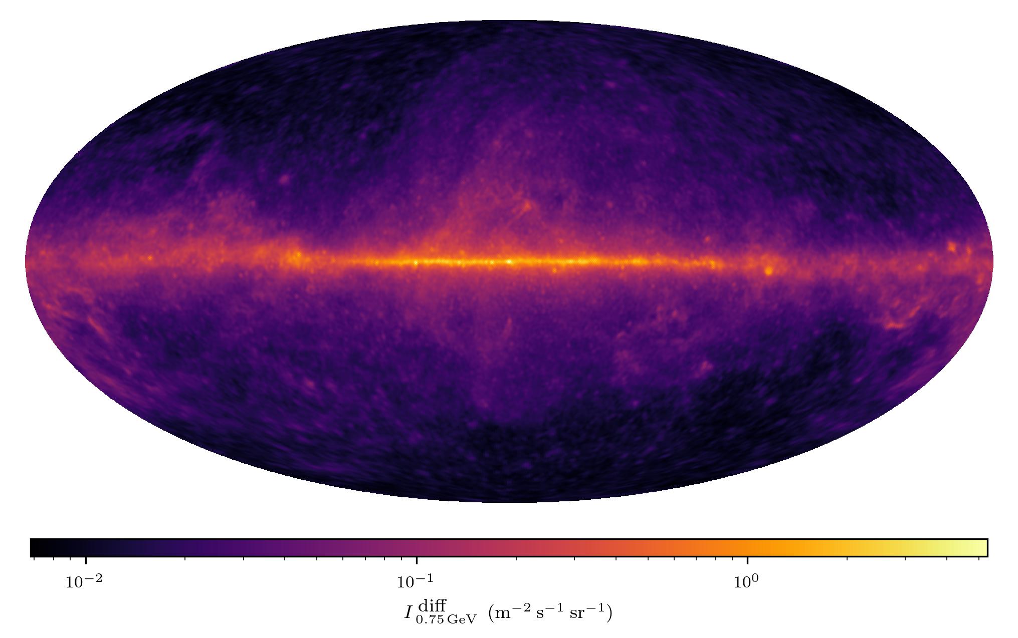
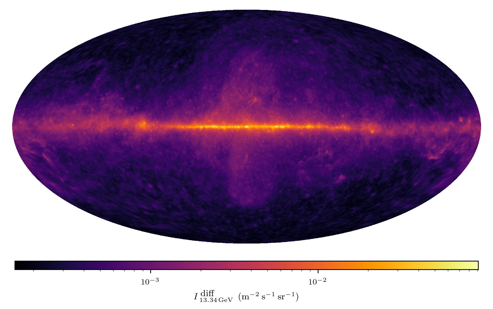
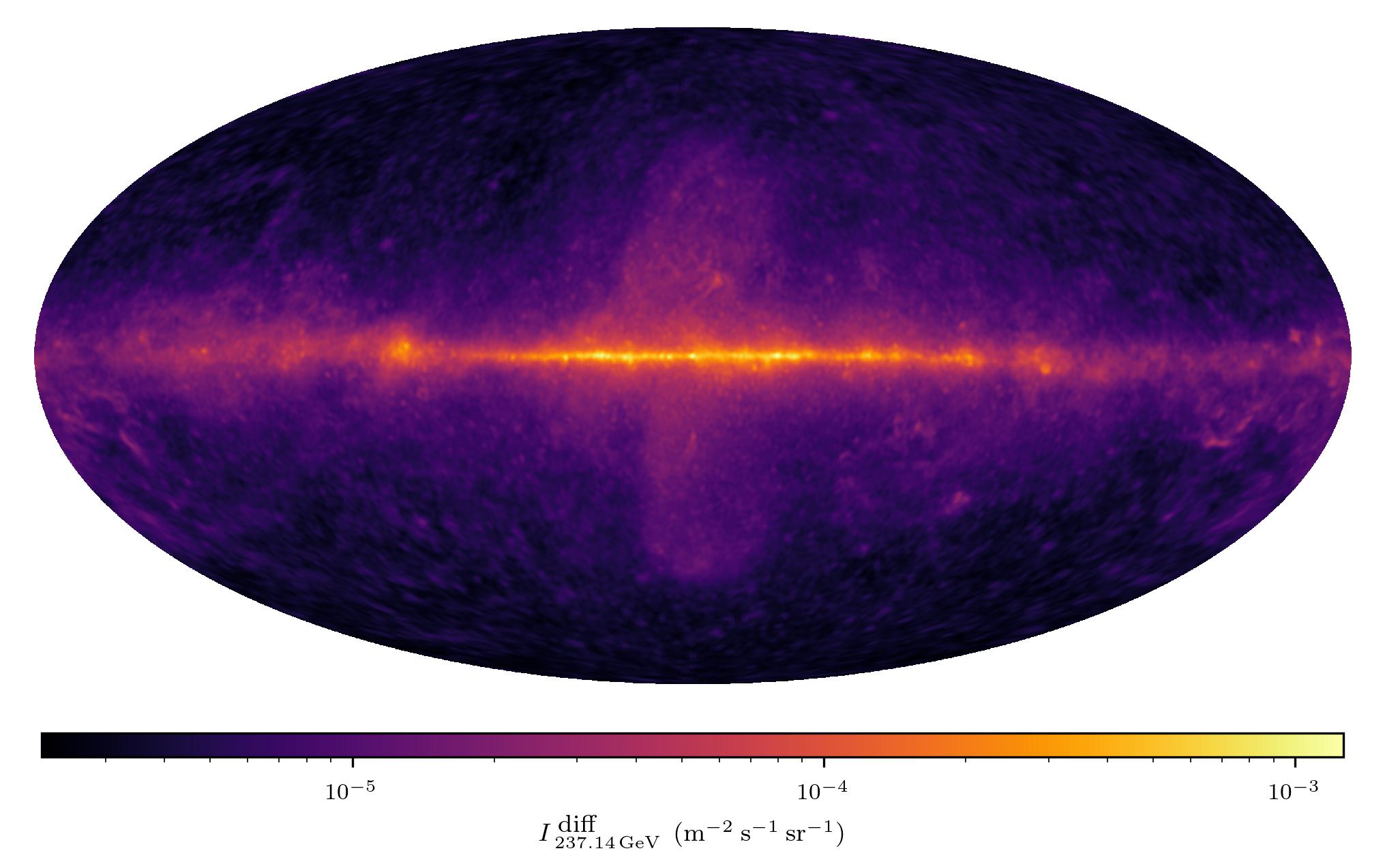
Figure 24: Single energy plots of the M1 diffuse reconstruction with a logarithmic color scale. Energy bins: 0.56–1.00 GeV (left), 10.0–17.8 GeV (middle), and 178–316 GeV (right). All panels have individual brightness scales and visualize the full dynamic range of their respective maps.

Figure 24 displays the M1 diffuse emission reconstruction in the 0.56–1.00 GeV, 10.0–17.8 GeV, and 178–316 GeV energy bins. The progression of maps shows the transition from a sky dominated by hadronic emission in the 1 GeV energy regime to one increasingly dominated by leptonic emissions in the 100 GeV energy regime, where the FBs and Galactic disk are visible as the most prominent structures. The corresponding M2 diffuse emission reconstruction maps are shown in Fig. 14.

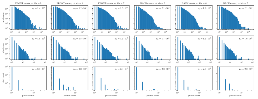
Figure 25: Histograms of data photon counts for all response bins with the energies 1.00–1.78 GeV (top), 10.0–17.8 GeV (middle), and 178–316 GeV (bottom). Photon counts and histogram pixel counts are shown on logarithmic scales. The number of pixels with zero observed photons, $\mathrm{n}_{0}$, is displayed as text in each panel. The apparent photon count sparsity in the $<$ 10 counts regime is caused by the sparsity of integer numbers on the logarithmic scale in that regime. Figure 4 shows the residual histograms of the selected bins.

Figure 25 shows the empirical distribution of photon counts in all response bins considered in this paper for the energy bins 1.00–1.78 GeV, 10.0–17.8 GeV, and 178–316 GeV. The counts in the 1.00–1.78 GeV energy bin follow a broken power law with an index of approximately -1.35 below the break at $1.5\cdot{10}^{2}$ ph and indices between -2.5 and -2.0 above the break. The existence of the break is consistent in all data response bins of this energy. In the 10.0–17.8 GeV energy bin the photon counts also follow a power law with an index of approximately -3.1 without an apparent break. The power-law behavior seems to also hold for the 178–316 GeV energy bins. Here, we refrain from calculating approximate power-law exponents as the low overall photon counts lead to high variability between the different response bins.

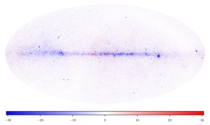
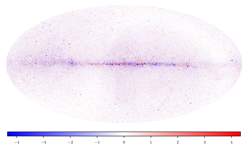
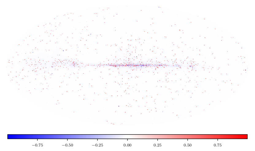
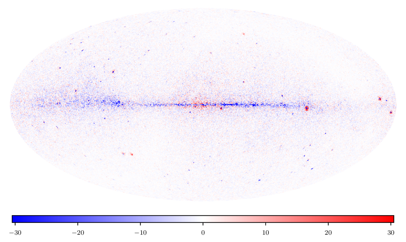
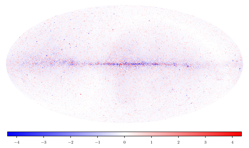
Figure 26: Selected residual maps for the M2 reconstruction shown for the data bin with $\cos(\theta_{\mathrm{w^{\prime}}})\in(0.9,1.0]$. Top: FRONT events. Bottom: BACK events. Energy bins: 1.00–1.78 GeV (left), 10.0–17.8 GeV (middle), and 178–316 GeV (right). The maps are clipped to the 99.9th percentile of the residual amplitude in their respective energy bin.

Figure 26 shows selected residuals of the reconstruction based on the M2 (template-informed) model. Similar to the residuals of the M1 reconstruction (see Fig. 5), the M2 residuals are largest in the Galactic plane and around extended sources such as Vela. We observe the same inversion of residuals between FRONT and BACK events around the brightest PSs, and a general agreement with the residuals of the M1 reconstruction.

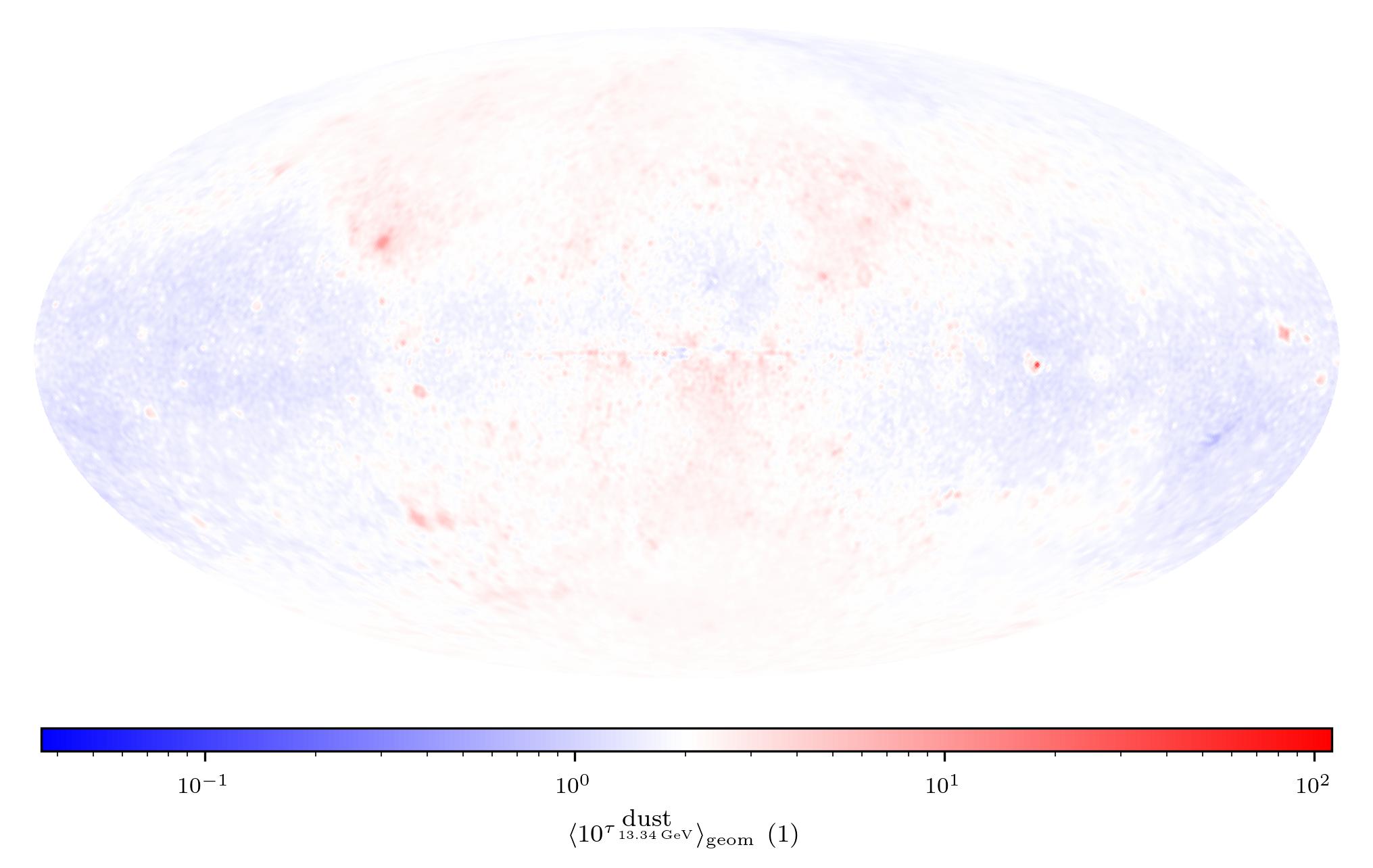
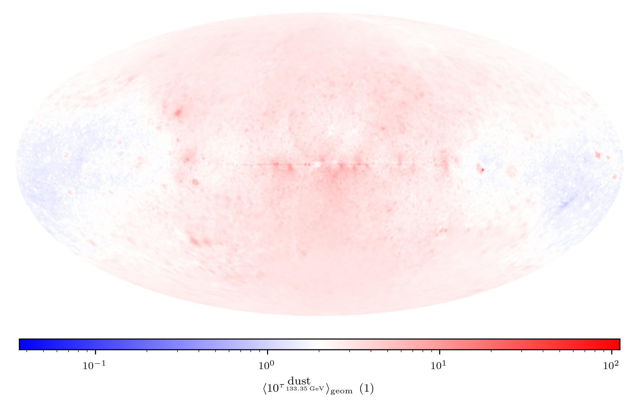
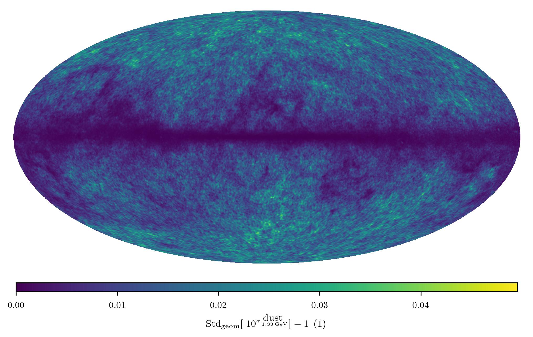
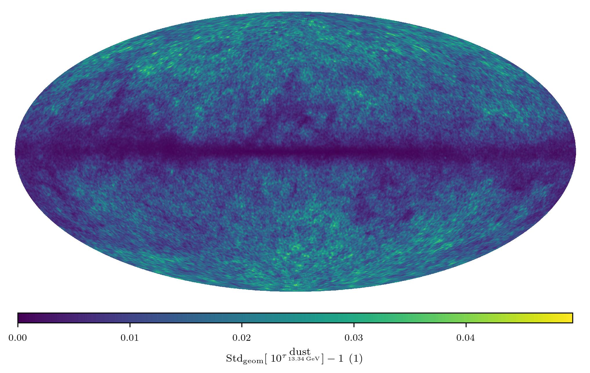
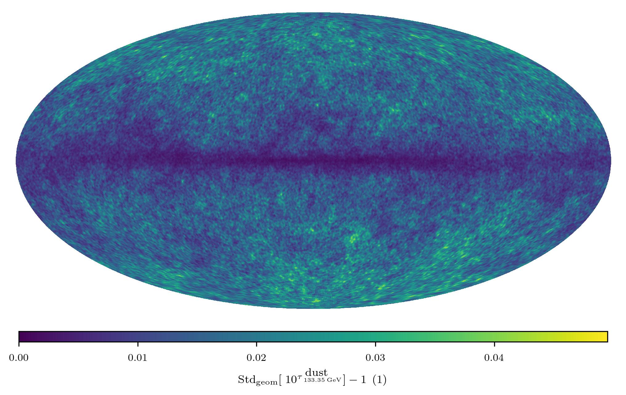
Figure 27: Posterior statistics of the M2 thermal dust template modification field for selected energy bins. Top row: Posterior mean of the multiplicative template modification fields on logarithmic color scales. Bottom row: Corresponding posterior multiplicative uncertainty of the modification fields on linear color scales. Energy bins: 1.0–1.78 GeV (left), 10.0–17.8 GeV (middle), and 100–178 GeV (right).

Figure 27 shows the modification field $\tau^{\mathrm{\>dust}}$ learned for the Planck thermal dust emission template in the M2 reconstruction run and the corresponding multiplicative uncertainty maps in the energy bins 1.0–1.78 GeV, 10.0–17.8 GeV, and 100–178 GeV. Toward higher energies, the average of the field increases slightly, indicating that the reconstruction preferred a harder spectrum than the prior encoded, which specifies a base power-law spectral index of $\alpha^{\mathrm{\>dust}}=-1.65$. The multiplicative uncertainty appears to be stable across the energy bands shown, but with regions of low multiplicative uncertainty in the 1.00–1.78 GeV and 10.0–17.8 GeV energy bins where the dust emissions predict the hadronic gamma-ray emissions to a high degree of accuracy.

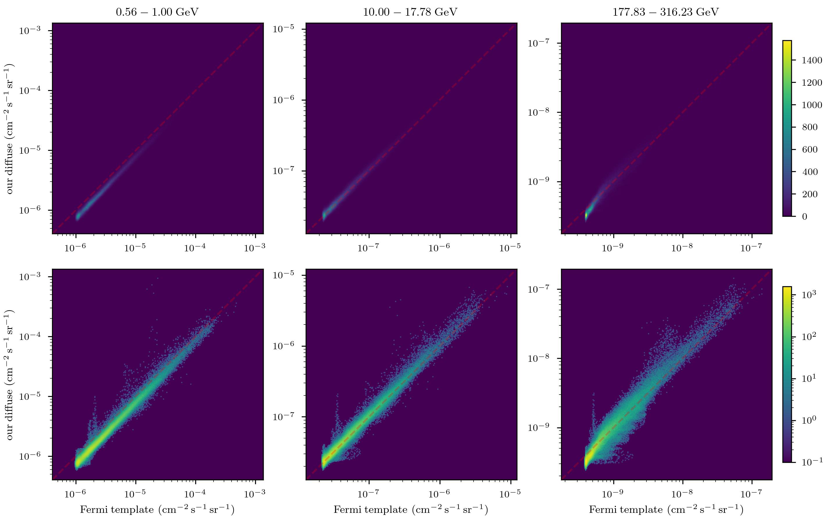
Figure 28: Comparison of the M2 diffuse reconstruction with the diffuse emission templates published by the Fermi Collaboration (diffuse foreground: gll_iem_v07, isotropic background: iso_P8R3_SOURCE_V3_v1). Left: 2D histograms of the diffuse flux found by our M2 reconstruction vs. the diffuse emission templates for the energy bins 0.56–1.00 GeV, 10.0–17.8 GeV, and 178–316 GeV. The histogram bins are logarithmically spaced in both fluxes. The top row shows the histogram counts with a linear color scale, while the bottom row shows them with a logarithmic color scale. The dashed red line marks perfect agreement. Right: Histogram of flux ratios (our diffuse reconstruction divided by the corresponding voxel values predicted by the template) for all spatio-spectral bins. Flux ratios are binned and displayed on a logarithmic scale. Numbers larger than $10^{0}$ indicate we reconstruct more flux than the template predicts.

Figure 28 shows the 2D histograms of fluxes in the Fermi diffuse emission templates and our M2 diffuse emission reconstruction. As already known from the comparison of the M1 and M2 reconstructions, the M2 reconstruction under-predicts diffuse emission in the lowest energy bin. This effect is visible in the top-left panel of Fig. 28 as an offset between the dotted red line and the line of high histogram counts. The corresponding panels for the M1 diffuse reconstruction are provided in Fig. 6.

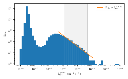
Figure 29: PS pixel count histogram for the M2 reconstruction on log-log scale. The orange line shows a power-law fit to the brightness distribution in the brightness range highlighted in gray. Flux values below $5\cdot{10}^{-7}$ $\mathrm{m}^{-2}\,\mathrm{s}^{-1}$ should be regarded as non-detections. The distribution function in this regime is prior-driven.

Figure 29 shows the SCD found for the PS pixels in the M2 reconstruction. It follows a similar shape as the SCD found with M1 (see Fig. 9). The M2 SCD follows a slightly steeper power law in the highlighted range. This might be an effect of the increased PS flux contribution in the M2 reconstruction compared with the M1 reconstruction. Point source pixels not or only slightly participating in the M1 reconstruction took on flux in the M2 reconstruction, increasing the ratio of low-flux but active PS pixels to high-flux PS pixels and thereby changing the SCD power-law index.

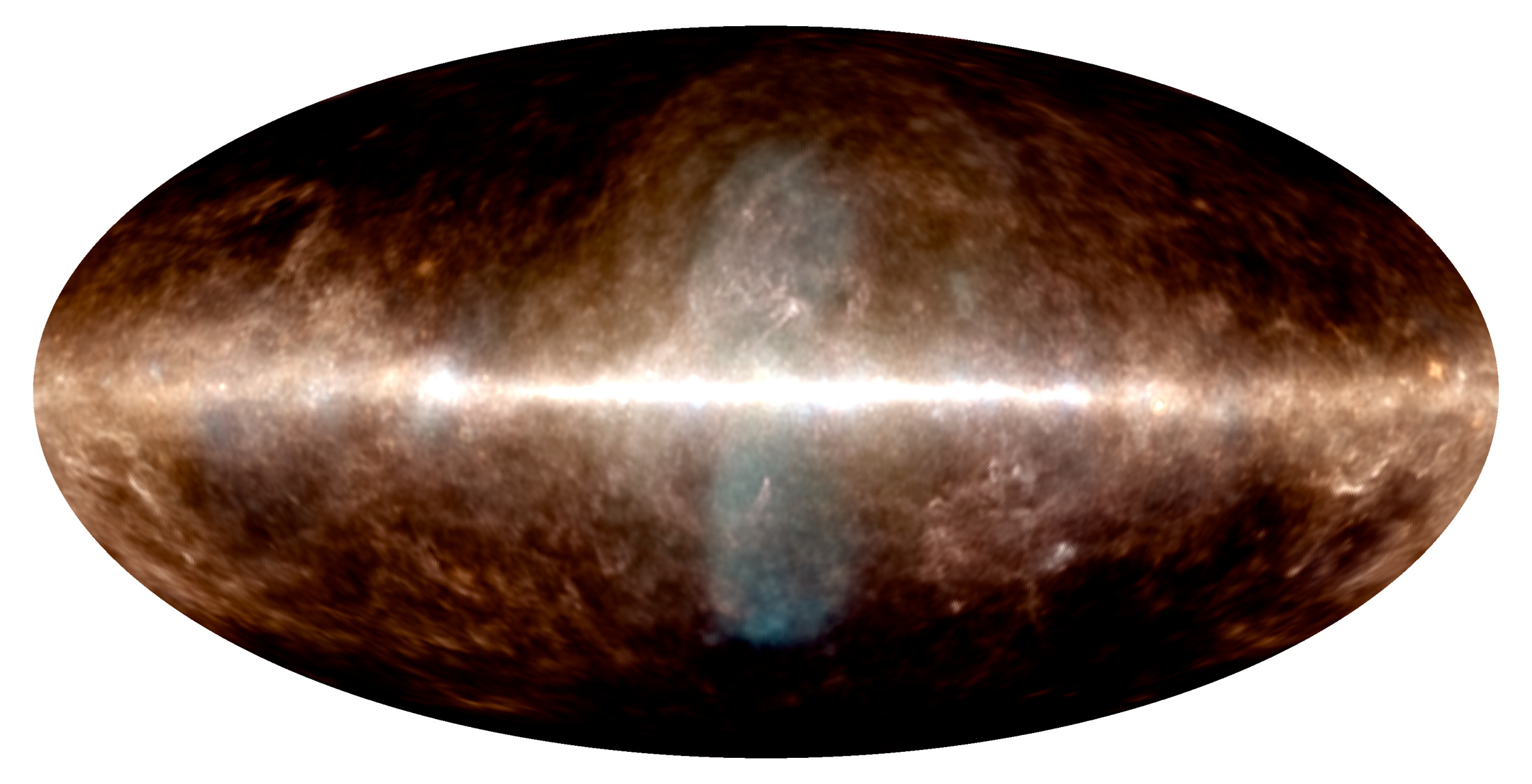
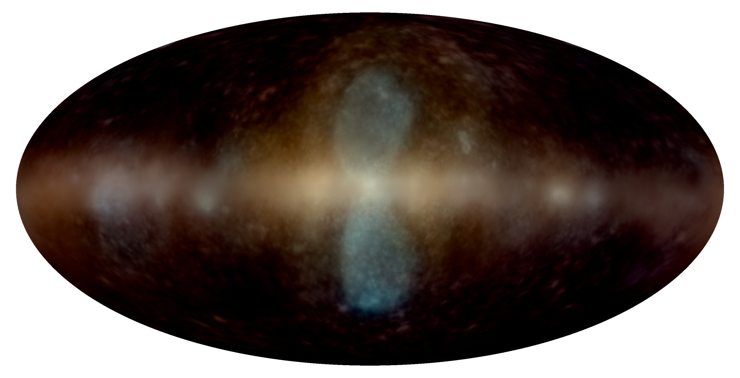
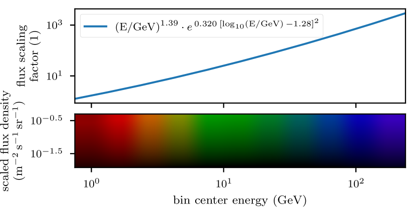
Figure 30: Spatio-spectral plotting without color saturation enhancement. The sky maps in the top and middle panel are based on the same color rendering as Fig. 2, 3, and 13, but were produced without the color saturation enhancement described in Appendix C. Top: Total diffuse emission reconstruction based on M2. Middle: Template-free diffuse emission $I^{\mathrm{\>nd}}$ reconstruction based on model M2. Bottom: Energy-dependent flux scaling factor (identical to Fig. 2) and mapping of photon energies and scaled flux densities to perceived colors without the color saturation enhancement.

Figure 30 shows the spatio-spectral emission maps for the total diffuse and template-free diffuse emission component of the M2 reconstruction without the color saturation enhancement described in Appendix C and the corresponding color mapping. These natural saturation maps are better suited to show fine structures than the saturation-enhanced maps displayed in Fig. 13, but because of their lower color saturation do not show spectral variations as clearly.