On the implementation of Adaptive and Filtered MHE

Abstract

Optimisation-based algorithms known as Moving Horizon Estimator (MHE) have been developed through the years. This paper illustrates the implementation of the policy introduced in the companion paper submitted to the 18th IFAC Workshop on Control Applications of Optimization (Oliva and Carnevale, 2022), in which we propose two techniques to reduce the computational cost of MHEs. These solutions mainly rely on output filtering and adaptive sampling. The use of filters reduces the total amount of data used by MHE, shortening the length of the moving window (buffer) and consequently decreasing the time consumption for plant dynamics integration. Meanwhile, the proposed adaptive sampling policy discards those sampled data that do not allow a sensible improvement of the estimation error. Algorithms and numerical simulations are provided to show the effectiveness of the proposed strategies.

Keywords Adaptive observer, Nonlinear systems, Moving Horizon Estimator

1 Introduction

Observer design represents a well-known task in control theory, playing a pivotal role in the controller design. A classic example of the interconnections of these two problems is described by the Separation Principle stated by Kalman in its most famous and elegant definition. As far as observers are concerned, many different approaches have been studied and developed over the years; from the most used linear algorithms like the Luenberger and Kalman observers (Davis, 2002; Thrun et al., 2006), up to more involved solutions for nonlinear systems (Thrun et al., 2006; Reif et al., 1999; Karagiannis et al., 2008; Karagiannis and Astolfi, 2005). Another topic of great interest in the field of observers is the adaptive approach, whose task consists in estimating model parameters too (Luders and Narendra, 1974; Krener and Isidori, 1983; Marino, 1990; Tyukin et al., 2013; Marine et al., 2001; Marino and Tomei, 1992). A fascinating approach addressing a general observation problem (both adaptive and non-adaptive) is the one proposed by the Moving Horizon Estimators (MHE) (Michalska and Mayne, 1995; P.E. Moraal, 1995; Kang, 2006; Wynn et al., 2014; Sui et al., 2010; Suwantong et al., 2014; Schiller et al., 2021). These are very powerful optimisation-based observers, but they suffer from computational cost issues. These issues make their online implementation quite hard to reach. To increase the computational speed, we propose in (Oliva and Carnevale, 2022) to exploit output-measurement filters to reduce the number of model integrations needed to solve the optimisation problem at the basis of standard MHE algorithms. Moreover, we propose an adaptive-sampling policy, making the observer capable of autonomously choosing the "best" measurements to be considered in the moving window buffer. The strategies proposed hinge upon MHE convergence analysis presented in (Aeyels, 1981; Kang, 2006; Glad, 1983; Menini et al., 2019, 2022).

This short work describes in detail the implementation of solutions proposed in (Oliva and Carnevale, 2022), presenting the Algorithms to implement the Filtered MHE and the Adaptive MHE and providing as well some simulation results. More specifically, in 2 the Standard MHE frameworks is described, while 3 treats both the Filtered MHE and Adaptive MHE cases. Conclusions are drawn in 4, as well as future developments.

2 Moving Horizon Estimators

Consider the general framework described in (Oliva and Carnevale, 2022), namely a nonlinear system in the following form

$$\dot{\bm{\xi}} =f(\bm{\xi},\bm{u})$$ (1a)

$$\bm{y} =h(\bm{\xi},\bm{u}).$$ (1b)

In this set of equations $\bm{\xi}\in\mathbb{R}^{n}$ is the state vector, $\bm{u}\in\mathbb{R}^{m}$ is the control input, and $\bm{y}\in\mathbb{R}^{p}$ is the measured output. From this general framework, in order to define the MHE, system (1) shall be considered in its N-lifted form. Accordingly to (P.E. Moraal, 1995) and (Tousain et al., 2001), and following the notation introduced in (Oliva and Carnevale, 2022), the N-lifted system generated from (1) is described by an output operator in the following form:

$$\text{H}_{k}(\bm{\xi}_{k-N+1},u(\cdot))\!=\!\!\!\begin{bmatrix}\!h(\bm{\xi}_{k-N+1},\bm{u}_{k-N+1})\\ \!h(\phi(t_{k-N+2},t_{k-N+1},\bm{\xi}_{k-N+1},\bm{u}(\cdot)),\bm{u}_{k-N+2})\\ \!\vdots\\ \!h(\phi(t_{k},t_{k-1},\bm{\xi}_{k-1},\bm{u}(\cdot)),\bm{u}_{k})\end{bmatrix},$$ (2)

where $(\text{Y}_{k},\text{U}_{k})$ are the output and input sample buffers of length $N$ and down-sampling $N_{T_{s}}$. Moreover, $\phi(t_{k};t_{k-1},\bm{\xi}_{k-1},\bm{u}(\tau))=\bm{\xi}(t_{k})=\bm{\xi}_{k}$ describes the solution of (1) at time $t_{k}$ with $\tau\in[t_{k-1},t_{k}]$, and $\bm{u}(t)$ is assumed to be a piece-wise constant function of the time, within sampling times of length $T_{s}$. Therefore, The MHE associated to (1) through its N-lifted system can be defined as

$$\bm{{\zeta}}_{i+1} =\bm{\Psi}(\text{Y}_{k},\text{U}_{k},\text{H}_{k}(\bm{{\zeta}}_{i},\bm{u}(\cdot)),\bm{\zeta}_{i}),$$ (3a)

$$\bm{\zeta}_{0} =\hat{\bm{\xi}}_{k-N+1},\text{ with, }i=0\dots K,\ K\in\mathbb{N},$$ (3b)

$$\hat{\bm{\xi}}_{k} =\phi(t_{k},t_{k-N+1},\bm{\zeta}_{K},\bm{u}(\cdot)),$$ (3c)

In this set of equations we consider $\hat{\bm{\xi}}_{k}$ as the estimated state vector of $\bm{\xi}_{k}$. Instead, $i$ is the iteration number of the optimisation algorithm defining the updated value of $\bm{\zeta}$. This value is computed through $\Psi$, that describes a general algorithm designed to solve optimisation problems (e.g. simplex or gradient-based solutions). This optimisation algorithm is iteratively launched within the intervals $[t_{k-1},t_{k}]$ for $K$ times. To sum up, the estimation problem at the basis of MHEs consists in finding the solution to the following minimisation problem:

$$\underset{\hat{\bm{\xi}}_{k-N+1}}{\text{min}}\text{V}_{k}(\text{Y}_{k},\text{U}_{k},\hat{\text{H}}_{k},\hat{\bm{\xi}}_{k-N+1}).$$ (4)

The cost $V_{k}$ has been defined as a quadratic function, namely

$$V_{k}(\text{Y}_{k},\text{U}_{k},{\text{H}}_{k},\zeta)\triangleq\sum\limits_{j=1}^{N}(\text{Y}_{k}^{j}-\hat{\text{H}}_{k}^{j})^{T}W_{j}(\text{Y}_{k}^{j}-\hat{\text{H}}_{k}^{j}),$$ (5)

where we considered the notation $\hat{H}_{k}=\text{H}_{k}(\hat{\bm{\xi}}_{k-N+1},$ $\bm{u}(\cdot))$. Moreover, $W_{i}\in\mathbb{R}^{p\times p}$ are symmetric and positive definite weight matrices and $(\text{Y}_{k}^{j},\hat{\text{H}}_{k}^{j})$ are the j-th rows of the matrices $Y_{k}$ and $\hat{H}_{k}$, respectively. For a detailed discussion on the Standard MHE structure of the optimisation problem solution and on its convergence properties, please refer to (Oliva and Carnevale, 2022). In addition to these considerations it is important to remark that if the plant dynamics (3a) are linear, then it is possible to consider the Newton algorithm yielding zero estimation error with just $K=2$ since $V_{k}$ is quadratic, and therefore resulting in the dead-beat observer described in (P.E. Moraal, 1995).

Lastly, with reference to the Standard MHE proposed in (Oliva and Carnevale, 2022), a more clear description of the algorithm is proposed in pseudo-code in 1. Remember that $K$ represents the number of optimisation steps performed by the optimisation algorithm $\bm{\Psi}$ chosen to solve (4). Moreover, note that the integral performed in the last algorithm step on the system model is computed numerically, as the analytical solution $\phi$ is not in general available in closed-form.

Algorithm 1 Standard MHE

for $t_{k}=k\cdot N_{T_{s}}\cdot T_{s}\in[t_{0},t_{f}]$ do

     

     $\triangleright$ Update buffers

     $\text{Y}_{k}[1:N-1]\leftarrow\text{Y}_{k}[2:N]$, $\text{U}_{k}[1:N-1]\leftarrow\text{U}_{k}[2:N]$

     $\text{Y}_{k}[N]\leftarrow y_{k}$, $\text{U}_{k}[N]\leftarrow u_{k}$

     

     $\triangleright$ Initialization of (3a)

     $\zeta_{0}\leftarrow\hat{\bm{\xi}}_{k-N+1}$

     

     $\triangleright$ Optimisation procedure

     for $i=0,\dots,K-1$ do

         $\zeta_{i+1}\leftarrow\bm{\Psi}(\text{Y}_{k},\text{U}_{k},\hat{\text{H}}_{k},\zeta_{i})$

     end for

     $\hat{\bm{\xi}}_{k-N+1}\leftarrow\zeta_{K}$

     

     $\triangleright$ Propagate the estimate evaluating (3c)

     for $i\leq N-1$ do

         $\hat{\bm{\xi}}_{k-N+1+i}\leftarrow\int\limits_{t_{k-N+i}}^{t_{k-N+1+i}}f(\hat{\bm{\xi}}(\tau),u(\tau))d\tau$

     end for

end for

$\triangleright$ Estimate at $t=t_{k+qT_{s}}\neq t_{k}$, with $q\in\mathbb{Z}$, $|q|<N_{T_{s}}$

$\hat{\bm{\xi}}(t)\leftarrow\int\limits_{t_{k}}^{t_{k}+qT_{s}}f(\hat{\bm{\xi}}(\tau),u(\tau))d\tau$

3 Strategies for computational efficiency

This section considers the Filtered MHE and Adaptive MHE described in (Oliva and Carnevale, 2022), and aims at better describing the code implementation. Moreover, some considerations regarding the estimation convergence are reported. Generally speaking the focus is on the role of parameters $N$ (buffer length) and $N_{T_{s}}$ (down-sampling). Some considerations will be explained by simulation results on two different models, the Van der Pol oscillator and a nonlinear system describing the dynamics of plasma waves in presence of runaway electrons (Buratti et al., 2021; Karagiannis et al., 2008).

Filtered MHE

As reported in (Oliva and Carnevale, 2022) a first solution to decrease the computational cost necessary to solve (4) consists in adding a filtered version of the system output measurements $y_{k}$. Roughly speaking, by increasing the conditions available at each time instants, the buffer length $N$ can be reduced. Results in this sense have been presented on a Van der Pol oscillator.

For the model setup and main results refer to (Oliva and Carnevale, 2022). The major effect of adding a filtering action on the output $y$ is that the filter state vector shall be propagated, updated and stored too during the optimisation process. Indeed, a general filter can be described as a discrete-time system, namely

$$\bm{\xi_{f}}(k+1) =\gamma(\xi_{f}(k),y(k)),$$ (6a)

$$y_{f}(k+1) =\beta(\bm{\xi_{f}}(k+1)),$$ (6b)

where $\bm{\xi_{f}}\in\mathbb{R}^{l}$ is the filter state, $y\in\mathbb{R}$ is the signal measurement to be filtered, and $y_{f}\in\mathbb{R}$ is the actual filtered signal. The pseudo-code relative to the Filtered MHE is presented in 2. The notation is the same used for Standard MHE.

Algorithm 2 Filtered MHE

for $t_{k}=k\cdot N_{T_{s}}\cdot T_{s}\in[t_{0},t_{f}]$ do

     

     $\triangleright$ Output filter

     $\bm{\xi_{f}}(k)\leftarrow\gamma(\bm{\xi_{f}}(k-1),y_{k})$

     $y_{k}^{f}\leftarrow\beta(\bm{\xi_{f}}(k))$

     $\overline{y}_{k}\leftarrow[y_{k}\ y_{k}^{f}]^{T}$

     

     $\triangleright$ Update buffers

     $\text{Y}_{k}[1:N-1]\leftarrow\text{Y}_{k}[2:N]$, $\text{U}_{k}[1:N-1]\leftarrow\text{U}_{k}[2:N]$

     $\text{Y}_{k}[N]\leftarrow\overline{y}_{k}$, $\text{U}_{k}[N]\leftarrow u_{k}$

     

     $\triangleright$ Initialization of (3a)

     $\zeta_{0}\leftarrow\hat{\bm{\xi}}_{k-N+1}$

     

     $\triangleright$ Optimisation procedure

     for $i=0,\dots,K-1$ do

         $\zeta_{i+1}\leftarrow\mathbf{\Psi}(\text{Y}_{k},\text{U}_{k},\hat{\text{H}}_{k},\zeta_{i})$

     end for

     $\hat{\bm{\xi}}_{k-N+1}\leftarrow\zeta_{K}$

     

     $\triangleright$ Propagate the estimate evaluating (3c)

     for $i\leq N-1$ do

         $\hat{\bm{\xi}}_{k-N+1+i}\leftarrow\int\limits_{t_{k-N+i}}^{t_{k-N+1+i}}f(\hat{\bm{\xi}}(\tau),u(\tau))d\tau$

         $\hat{\bm{\xi}}_{\bm{f}}(k-N+1+i)\leftarrow\sum\limits_{i=k-N+i}^{k-N+1+i}\gamma(\hat{\bm{\xi}}_{\bm{f}}(i),\hat{y}_{i})$

     end for

end for

$\triangleright$ Estimate at $t=t_{k+qT_{s}}\neq t_{k}$, with $q\in\mathbb{Z}$, $|q|<N_{T_{s}}$

$\hat{\bm{\xi}}(t)\leftarrow\int\limits_{t_{k}}^{t_{k}+qT_{s}}f(\hat{\bm{\xi}}(\tau),u(\tau))d\tau$

$\hat{\bm{\xi}}_{\bm{f}}(k+q)\leftarrow\sum\limits_{i=k}^{k+q}\gamma(\hat{\bm{\xi}}_{\bm{f}}(i),\hat{y}_{i})$

Adaptive MHE

The second solution proposed in (Oliva and Carnevale, 2022) to speed up MHEs implementation consists in defining a policy according to which the observer can automatically select the output measurements that are most informative for the solution of (4). This selection is done accordingly to the following indices $\delta_{k}$ and $d_{\text{V}}$, that are a good representative of the output signal richness as well as the precision of the estimate:

$$\Sigma_{k} =\{\sigma_{i}\triangleq\left\lVert\text{Y}_{k}^{i+1}-\text{Y}_{k}^{i}\right\rVert\ \text{ s.t. }i\in[1,\dots,N-1]\},$$ (7a)

$$\delta_{k} =\sum\limits_{i=1}^{N-1}\sigma_{i}+\left\lVert y_{k}-\text{Y}_{k}^{1}\right\rVert,$$ (7b)

$$d_{\text{V}} =\left\lVert\text{Y}_{k}-\hat{\text{H}}_{k}\right\rVert.$$ (7c)

The adaptive policy is implemented by thresholding both $\delta_{k}$ and $d_{\text{V}}$ and deciding whether to run or not the estimation accordingly. Moreover, if no estimation is performed for a long time due to a high precision reached, the output buffer is re-initialised to avoid excessively time-consuming model integrations (Parameter $N_{\text{max}}$ (Oliva and Carnevale, 2022)). Again, the pseudo-code relative to the Adaptive MHE is presented in 3. Results have been presented on the following model, describing the dynamics of plasma waves amplitude ($\xi_{1}$) and anisotropy of the runaway electrons velocity distribution ($\xi_{2}$) given by (Buratti et al., 2021):

$$\dot{\xi}_{1} =\epsilon(-2\xi_{1}\xi_{2}-2S+Q),$$ (8a)

$$\dot{\xi}_{2} =\epsilon(-\nu\xi_{2}+\xi_{3}(\xi_{1}\xi_{2}+S)-\gamma_{1}\dfrac{\xi_{2}}{1+\dfrac{\xi_{2}}{W_{t}}}),$$ (8b)

$$\dot{\xi_{3}} =0,$$ (8c)

$$y =\xi_{2},$$ (8d)

where $y\in\mathbb{R}$ is the output, $\bm{\xi}\in\mathbb{R}^{3}$ is the state vector. Figure 1 shows the actual measurement samples, when different values of fixed $N_{T_{s}}$ are considered, namely $N_{T_{s}}=5$ and $N_{T_{s}}=38$. As reported in (Oliva and Carnevale, 2022), when $N_{T_{s}}=38$, index $\delta_{k}$ is low and the state is not correctly estimated. Indeed, this means that the sampled trajectory is not highly informative. This can be clearly seen in Figure 1 where the blue circles have a nearly null value compared to the general trend of the trajectory. Clearly, an informative set of measurements shall be sampled over the trajectory peaks, rather than on the flat and dense intervals between them.

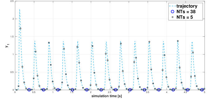
Figure 1: This figure compares the system trajectory (dashed line) and the sampled measurements when $N_{T_{s}}=5$ (squares) and $N_{T_{s}}=38$ (circles).

The results of the actual Adaptive MHE are presented in Figure 2. The simulation follows the very same setup considered in (Oliva and Carnevale, 2022). Note how the sampling is now concentrated at the beginning of the simulation and on the peaks, in order to quickly reduce the estimation error and then correct the estimation when the measurements were informative enough. Whenever the estimation error increases, the observer samples the output in correspondence of those trajectory regions in which the signal richness is higher. The estimation precision is comparable to the Standard MHE, yet significantly reducing the computational cost.

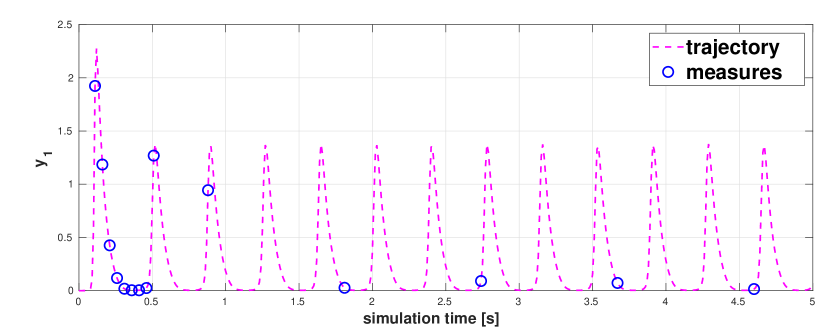
Figure 2: This figure shows the true state trajectory for system (8) (black dashed line), and the sampled measures provided to the observer when the adaptive sampling policy is used (blue big circles).

Algorithm 3 Adaptive MHE

for $t_{k}=k\cdot N_{T_{s}}\cdot T_{s}\in[t_{0},t_{f}]$ do

$\triangleright$ Adaptive sampling

     if AC1 $\And$ AC2 then

         

         $\triangleright$ Check max spacing

         if $T(y_{k})-T(\text{Y}_{k}^{N})\geq N_{\max}$ then

              

              $\triangleright$ Re-initialise buffer

              for $i\leq N$ do

                  $\text{Y}_{k}^{i}=y_{k-N+i}$

              end for

         else

              

              $\triangleright$ Update buffers

              $\text{Y}_{k}[1:N-1]\leftarrow\text{Y}_{k}[2:N]$

              $\text{U}_{k}[1:N-1]\leftarrow\text{U}_{k}[2:N]$

              $\text{Y}_{k}[N]\leftarrow y_{k}$, $\text{U}_{k}[N]\leftarrow u_{k}$

         end if

         

         $\triangleright$ Initialization of (3a)

         $\zeta_{0}\leftarrow\hat{\bm{\xi}}_{k-N+1}$

         

         $\triangleright$ Optimisation procedure

         for $i=0,\dots,K-1$ do

              $\zeta_{i+1}\leftarrow\mathbf{\Psi}(\text{Y}_{k},\text{U}_{k},\hat{\text{H}}_{k},\zeta_{i})$

         end for

         $\hat{\bm{\xi}}_{k-N+1}\leftarrow\zeta_{K}$

         

         $\triangleright$ Propagate the estimate evaluating (3c)

         for $i\leq N-1$ do

              $\hat{\bm{\xi}}_{k-N+1+i}\leftarrow\int\limits_{t_{k-N+i}}^{t_{k-N+1+i}}f(\hat{\bm{\xi}}(\tau),u(\tau))d\tau$

         end for

     end if

end for

$\triangleright$ Estimate at $t=t_{k+qT_{s}}\neq t_{k}$, with $q\in\mathbb{Z}$, $|q|<N_{T_{s}}$

$\hat{\bm{\xi}}(t)\leftarrow\int\limits_{t_{k}}^{t_{k}+qT_{s}}f(\hat{\bm{\xi}}(\tau),u(\tau))d\tau$

Filtered and Adaptive MHE

This last section focuses on the joint action of Filtered MHE and Adaptive MHE. In fact, Filtered MHE reduces the computational speed of each optimisation solution of (4), while Adaptive MHE reduces the number of optimisation required to reach a good estimation precision. Therefore, if both 2 and 3 were used in combination, namely exploiting both output filtering and adaptive sampling, we would both decrease the single optimisation time and the total number of performed optimisations. Indeed, the speed up factor would be even greater.

In order to test the performance of both output filtering and adaptive sampling we combined the Filtered MHE and the Adaptive MHE on a double pendulum, considering $K=40$ and two output filter, namely a dirty-derivative and an integrator with loss [cfr. Oliva et al. 2022]. The model considered for this set of simulations consists of a double pendulum. The general structure of the equations resembles the usual model used in robotics, namely

$$\mathbb{M}(q)\ddot{q}+\mathbb{V}(q,\dot{q})\dot{q}+\mathbb{G}(q)=\tau,$$ (9)

where $q=(\theta_{1},\theta_{2})$ are the angular positions of the links, the $\mathbb{M}$ term describes the system inertia, the $\mathbb{V}(q,\dot{q})$ term the friction and Coriolis effects, and $\mathbb{G}(q)$ the gravitational force. Each pendulum was considered with length $L=1m$, and mass $M=1kg$. The system state is $\bm{\xi}=[q_{1},q_{2},\dot{q}_{1},\dot{q}_{2}]\in\mathbb{R}^{4}$, while the output measurement is $y=q_{1}\in\mathbb{R}$. The estimation error norm is presented in logarithmic scale in Figure 3.

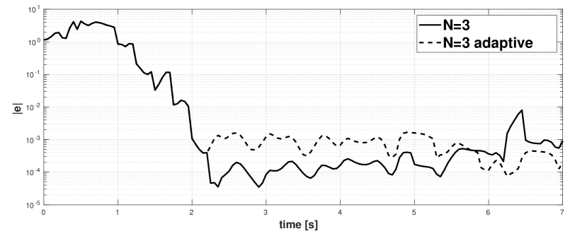
Figure 3: This figure shows the estimation error on both the filtered (solid line) and filtered-adaptive sampling (dashed line) cases on system (9) estimation.

The registered total computation time was $25.4$s for the joint action of Filtered MHE and Adaptive MHE which is nearly $60\%$ lower than the simple Filtered MHE case reported in (Oliva and Carnevale, 2022).

4 Conclusions and future work

This work builds on the results presented in (Oliva and Carnevale, 2022). In the first section 2, the Standard MHE structure was recalled and presented more accurately in pseudo-code layout. Moreover, some remarks on the convergence properties introduced in (Oliva and Carnevale, 2022) are reported. More specifically, the special case of an MHE turning into a dead-beat observer has been considered. In 3 the solutions proposed in (Oliva and Carnevale, 2022) to speed up MHE are considered. More specifically, the importance of filter propagation is stressed, and the Filtered MHE is presented in pseudo-code. As far as Adaptive MHE is concerned, the simulation results on plasma dynamics model described in (Oliva and Carnevale, 2022) are consolidated with some considerations on both the fixed and adaptive sampling policies. Lastly, the Adaptive MHE is presented in pseudo-code as well.

Future developments of this tool will consider a detailed analysis of the effect of measurement noise and model uncertainties on the observer performance and selection of filters. Another interesting point to be developed is using this tool for control laws design, relating it to the general MPC solution. Indeed, output tracking problems could be solved by including control parameters in the augmented state. For instance, classic MRAC or state feedback frameworks could be reproduced. Clearly, this application shall be considered as separated from the state estimation problem, because no separation principle is available for nonlinear systems.

Acknowledgemts

Thanks to Corrado Possieri and Mario Sassano for their comments and fundamental insights into the development of this work.

References

- Oliva and Carnevale [2022] Federico Oliva and Daniele Carnevale. Moving horizon estimator with filtering and adaptive sampling. submitted to the 18th IFAC Workshop Control Applications for Optimisation, 2022.
- Davis [2002] Jon H. Davis. Luenberger Observers, pages 245–254. Birkhäuser Boston, 2002.
- Thrun et al. [2006] S. Thrun, W. Burgard, and D. Fox. Probabilistic Robotics. The MIT Press, 2006.
- Reif et al. [1999] K. Reif, S. Gunther, E. Yaz, and R. Unbehauen. Stochastic stability of the discrete-time extended kalman filter. IEEE Transactions on Automatic Control, 1999.
- Karagiannis et al. [2008] Dimitrios Karagiannis, Daniele Carnevale, and Alessandro Astolfi. Invariant manifold based reduced-order observer design for nonlinear systems. IEEE Transactions on Automatic Control, 2008.
- Karagiannis and Astolfi [2005] D. Karagiannis and A. Astolfi. Nonlinear observer design using invariant manifolds and applications. In Proceedings of the 44th IEEE Conference on Decision and Control, 2005.
- Luders and Narendra [1974] G. Luders and K. Narendra. A new canonical form for an adaptive observer. IEEE Transactions on Automatic Control, 1974.
- Krener and Isidori [1983] Arthur J. Krener and Alberto Isidori. Linearization by output injection and nonlinear observers. Systems & Control Letters, 1983.
- Marino [1990] R. Marino. Adaptive observers for single output nonlinear systems. IEEE Transactions on Automatic Control, 1990.
- Tyukin et al. [2013] Ivan Y. Tyukin, Erik Steur, Henk Nijmeijer, and Cees van Leeuwen. Adaptive observers and parameter estimation for a class of systems nonlinear in the parameters. Automatica, 2013.
- Marine et al. [2001] R. Marine, G.L. Santosuosso, and P. Tomei. Robust adaptive observers for nonlinear systems with bounded disturbances. IEEE Transactions on Automatic Control, 2001.
- Marino and Tomei [1992] R. Marino and P. Tomei. Global adaptive observers for nonlinear systems via filtered transformations. IEEE Transactions on Automatic Control, 1992.
- Michalska and Mayne [1995] H. Michalska and D.Q. Mayne. Moving horizon observers and observer-based control. IEEE Transactions on Automatic Control, 1995.
- P.E. Moraal [1995] J.W. Grizzle P.E. Moraal. Observer design for noninear systems with discrete-time measurements. IEEE Transactions on Automatic Control, 1995.
- Kang [2006] Wei Kang. Moving horizon numerical observers of nonlinear control systems. IEEE Transactions on Automatic Control, 2006.
- Wynn et al. [2014] Andrew Wynn, Milan Vukov, and Moritz Diehl. Convergence guarantees for moving horizon estimation based on the real-time iteration scheme. IEEE Transactions on Automatic Control, 2014.
- Sui et al. [2010] Dan Sui, Tor Arne Johansen, and Le Feng. Linear moving horizon estimation with pre-estimating observer. IEEE Transactions on Automatic Control, 2010.
- Suwantong et al. [2014] Rata Suwantong, Sylvain Bertrand, Didier Dumur, and Dominique Beauvois. Stability of a nonlinear moving horizon estimator with pre-estimation. In 2014 American Control Conference, 2014.
- Schiller et al. [2021] Julian D. Schiller, Sven Knüfer, and Matthias A. Müller. Robust stability of suboptimal moving horizon estimation using an observer-based candidate solution. IFAC-PapersOnLine, 2021.
- Aeyels [1981] D. Aeyels. On the number of samples necessary to achieve observability. Systems & Control Letters, 1981.
- Glad [1983] S. T. Glad. Observability and nonlinear dead beat observers. In The 22nd IEEE Conference on Decision and Control, 1983.
- Menini et al. [2019] Laura Menini, Corrado Possieri, and Antonio Tornambè. Observers for linear systems by the time integrals and moving average of the output. IEEE Transactions on Automatic Control, 2019.
- Menini et al. [2022] Laura Menini, Corrado Possieri, and Antonio Tornambe. On the use of the time-integrals of the output in observer design for nonlinear autonomous systems. IEEE Transactions on Automatic Control, 2022.
- Tousain et al. [2001] R. Tousain, E. van der Meche, and O. Bosgra. Design strategy for iterative learning control based on optimal control. Proceedings of the 40th IEEE Conference on Decision and Control (Cat. No.01CH37228), 2001. doi:10.1109/CDC.2001.980905.
- Buratti et al. [2021] P Buratti, W Bin, A Cardinali, D Carnevale, C Castaldo, O D’Arcangelo, F Napoli, G L Ravera, A Selce, L Panaccione, and et al. Fast dynamics of radiofrequency emission in ftu plasmas with runaway electrons. Plasma Physics and Controlled Fusion, 2021.