The radio signal of PSR B0950$+$08 is detected over the whole pulse phase

Abstract

Pulsars are the “lighthouses” in the universe. Periodic pulses with the duty-cycle $\sim 10\%$ are detected when the radio beam of the rotating pulsar sweeps across the telescope. In this report, the 160 min-data of a nearby pulsar, PSR B0950$+$08, observed with the Five-hundred-meter Aperture Spherical radio Telescope (FAST) is analysed. Thanks to the extremely high sensitivity of FAST, it is found that the radiation of PSR B0950$+$08 could be detected over the entire pulse period. To investigate the radiative characteristics of the pulsar’s “bridge emission”, a function, $\Theta(n)$, is defined to reveal the weak radiation there. It is suggested that the narrow peaks of both the main and the inter pulses could be radiated at low altitude, while other weak emission (e.g., the “bridges”) from upper magnetosphere though its radiative mechanism is still a matter of debate. The measured mean pulse behaviors are consistent with previous results in the phase of strong emission of this pulsar, and both the frequency-independent separation between the inter-pulse and main pulse and the narrow pulse width may support a double-pole model. In order to understand the magnetospheric geometry of this pulsar, further polarization calibrated observation with FAST and a proper determination of the baseline emission, especially during the weak emission phase, are surely required.

1 Introduction

The nearby, bright pulsar, PSR B0950$+$08, is well known, with a spin period of 253 ms and dispersion-measure (DM) of 2.97 pc/cm³. Abundant observations have already been obtained for this normal pulsar (e.g. Hankins et al., 1991; Kuzmin et al., 1998; Everett & Weisberg, 2001; Shabanova & Shitov, 2004; Johnston et al., 2005). For instance, the averaged pulse profile of PSR B0950$+$08 shows frequency-dependent properties (e.g. Hankins et al., 1991; Kuzmin et al., 1998), and Shabanova & Shitov (2004) reported that the frequency dependent sinusoidal modulation of the pulse shape may result from the Faraday rotation effect. Also, its linear polarization is shown in the literature (e.g. Everett & Weisberg, 2001; Shabanova & Shitov, 2004; Johnston et al., 2005), but is too low to fit the polarization position angle (PPA) at the main pulse longitude by typical ’S’ shape in the Rotating Vector Model (RVM, Radhakrishnan & Cooke, 1969). In fact,  Everett & Weisberg (2001) presented the RVM fitting for PSR B0950$+$08. When they fitted the PPA of the whole pulse longitudes (Fig.8), the longitude range (-10,+15)^∘ of distortion regions appearing at the main pulse must be unweighted.  Popov et al. (2002) confirmed the characteristic timescales of micro-structure and narrow micro-structure are orders of 0.1 ms and 10 $\mathrm{\mu}$s, respectively, while the timescale of fine structure is $\sim 1$ ms (Ulyanov et al., 2016). Besides, the separation between inter-pulse and main pulse is frequency independent below 5 GHz, and this feature demonstrates that multi-pole magnetic field may contribute significantly in order to understand the “bridge” emission (Hankins & Cordes, 1981; Nowakowski et al., 2002).

In addition to the mean pulse profile, the single pulse behaviors have been studied for PSR B0950$+$08. After a detailed study of intensity dependence of individual pulses,  Nowakowski et al. (2002) found a possible correlation between the intensities and locations of the inter-pulse with the leading component of the main pulse. Additionally, PSR B0950$+$08 also exhibits the nulling pulse phenomenon and the sharp flux variation in a short-time scale (e.g. Cairns, 2004; Shabanova & Shitov, 2004; Singal & Vats, 2012). Besides, the giant pulse and giant micro-pulse phenomena have also been detected from PSR B0950$+$08 (e.g. Cairns, 2004; Singal & Vats, 2012; Tsai et al., 2015), but the origin of them is still a mystery.

Nevertheless, both properties of the mean pulse and single pulse would be significantly influenced by the baseline determination. The conventional baseline subtraction is to subtract the weak emission region away from the strong emission phase (i.e., the main pulse) of pulsar. If this baseline subtraction is directly used to subtract the weak emission region of the pulsar with unusually wider pulse such as PSR B0950$+$08, the impulsive radio signal of the weak emission phase of this pulsar is also subtracted. More details on the discussion of the baseline will also be presented in the latter section.  Hankins & Cordes (1981) strongly supported the conclusion that the radio emission from PSR B0950$+$08 occurs over at least $83\%$ of the rotation period. They pointed that, because of limited sensitivity of telescope, the radio emission characters of the “two minimum levels” at the bridge regions between inter-pulse and main pulse (the remaining $17\%$ pulse longitude) could not be defined with certainty.

Up to now, similar properties have also been discovered in PSR B1929$+$10 and some other millisecond pulsars (e.g. McLaughlin & Rankin, 2004; Dai et al., 2015), for all these pulsars it has been reported that the emission covers an unusually wide range of pulse longitude. Therefore, the radio emission of the whole pulse phase for these pulsars is worth detecting.  Navarro et al. (1995) discovered a binary millisecond pulsar, PSR J0218$+$ 4232, with the extremely broad pulse profile during imaging observations, they later confirmed that this pulsar exhibits a significant fraction of the radio emission is not pulsed. Meanwhile,  Ruan et al. (2020) reported the detection result of the emission features of off-pulse emission (the emission is non-periodic and stationary) from PSR B0950$+$08. Through imaging analysis, they concluded that the off-pulse emission of this pulsar is mainly originated from the outside of the magnetosphere. Nevertheless, it is hard to completely rule out the possibility of magnetospheric origin for off-pulse emission via imaging. The difference between the emission origins from inside and outside of the magnetosphere is whether the radiation is impulsive and periodic, and in this work, the impulsive characteristic of PSR B0950$+$08 is attempted to be detected. However, not all radio pulsars have off-pulse emission,  Marcote et al. (2019) presented a detailed detection of off-pulse emission for B0525$+$21 and B2045$-$16. They reported that the off-pulse emission above three times the rms noise levels for B0525$+$21 and B2045$-$16 are not detected using the European VLBI Network. The imaging method is potentially used to determine the pulsars with wide pulse profile such as PSR B1929$+$10 in the future.

The largest single-dish radio telescope in the world, china’s FAST would be an appropriate tool to understand more about radio emission as well as the radiative mechanism of PSR B0950$+$08, taking advantage of its extremely high sensitivity (Jiang et al., 2019, 2020). New scientific achievements have already been obtained with FAST, including studies of pulsars (e.g. Lu et al., 2019) and fast radio bursts (e.g. Xu, 2021). In this article, the emission from the “bridge” of PSR B0950$+$08 is determined (as shown in Fig. 1), exhibiting a concave structure. In this paper, a detailed study of the radiation properties of the entire $360^{\circ}$-pulse longitude is presented. The observations with FAST and the data reduction are described in Section 2. To determine the emission at the entire pulse period, a depth data analysis and the radiation characteristics of this pulsar are presented in Section 3. Finally, general conclusion and discussions are provided in Section 4.

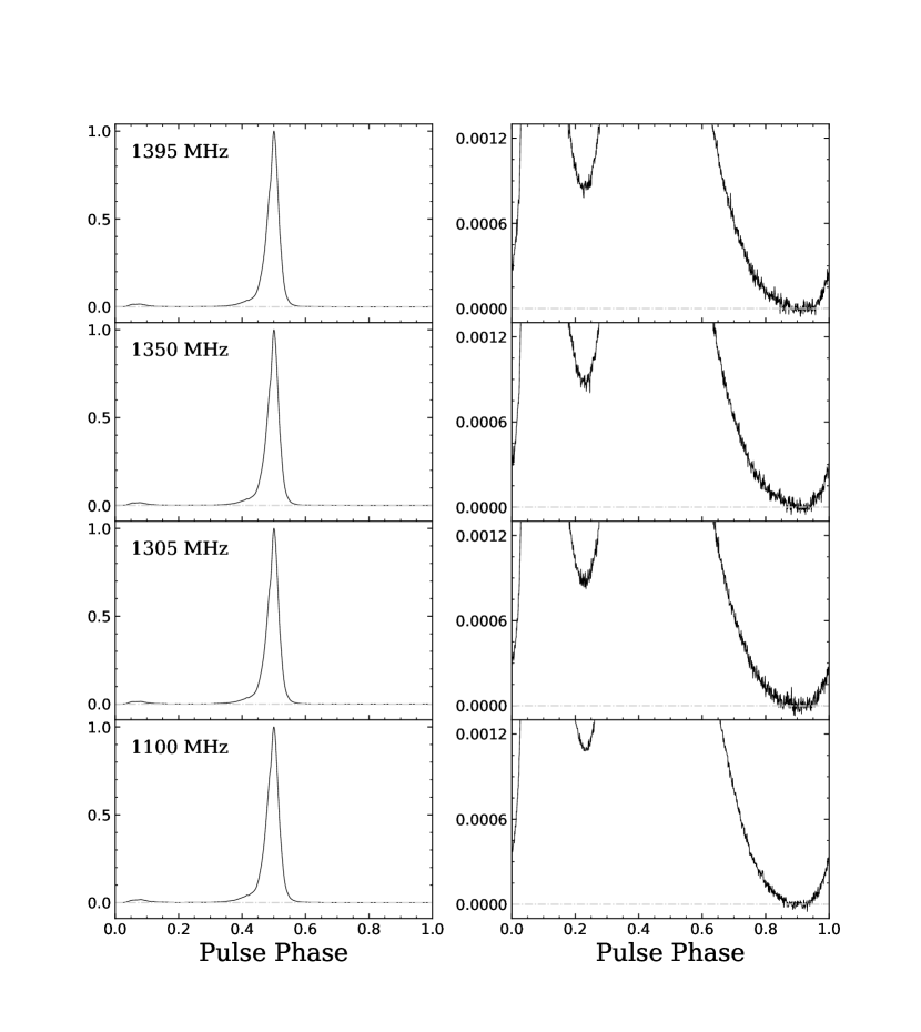
Figure 1: The averaged pulse profile at 1100, 1305, 1350, and 1395 MHz are shown in the left panel, and the corresponding $\times$800 expanded scale views are plotted in the right panels. The emission region of the pulse phase from 0.88 to 0.92 is regarded as the baseline region.

2 OBSERVATION AND DATA REDUCTION

FAST is located in Guizhou, a southwestern province of China, at longitude $106.9^{\circ}$ E and latitude $25.7^{\circ}$ N. In this work, the 19-beam receiver system was adopted. The central frequency and bandwidth of the receiver are 1250 and 400 MHz, respectively (Jiang et al., 2019, 2020). The system temperature of the 19-beam receiver is less that 24 K for central beam, and the system stability for most observation modes with the observation zenith angle less than $26.4^{\circ}$, is $\sim 1\%$ over 3.5  hours (Jiang et al., 2019, 2020)

In this work, PSR B0950$+$08 was observed with tracking mode on MJD 59396 (July 1st, 2021). The data were recorded as the 8 bit-sampled search mode PSRFITS format (Hotan et al., 2004) with 4096 frequency channels, and the frequency resolution is $\sim$ 0.122MHz. The entire integration time is 160 minutes, and the time resolution is $\sim$ 50 $\mathrm{\mu}$s. The DSPSR software package (van Straten & Bailes, 2011) was adopted in the data reduction, and the individual pulses were generated with 1024 phase bins across the pulse period of 253 ms (Hobbs et al., 2004).

To ensure that the radio signal of the weak emission region of PSR B0950$+$08 is not affected by the radio frequency interference (RFI), the RFI is detected using the dynamic spectrum. Significant and possible impulsive RFIs are eliminated. Moreover, the narrow-band RFI is also efficiently mitigated by using the dynamics spectrum. Then only the integrated sub-band data with frequencies of 1100, 1305, 1350, and 1395 MHz is remained, and their bandwidth are 80, 50, 40, and 50 MHz, respectively.

In this work, in order to obtain the averaged pulse profile and to discuss the radiation characteristics of strong emission phase of PSR B0950$+$08, the emission region of the pulse phase from 0.88 to 0.92 (see Figs. 1 and 2) is regarded as the baseline region and then subtract it. Furthermore, to detect the pulsed radio signal of the “bridge” emission region of this pulsar. The baseline in each single pulse can be determined according to the pulsed radio emission in each individual pulse is narrow pulse. After the baseline subtraction i.e., subtracting the receiver contribution is carried out in each single pulse, and the radio emission caused by the systematic contribution is unpulsed. The systematic contribution of the “bridge” emission region is removed by the impulsive property of the sub-pulse of this pulsar. More detailed detection of the pulsed radio signal across the whole pulse phase will be presented in the Section 3 and  4.

3 DATA ANALYSIS AND RADIATION CHARACTERISTICS

In order to discuss the emission characteristics of PSR B0950+08, the emission from the 0.17 to 0.30 and 0.65 to 0.95 pulse phase intervals in Fig. 3, which is called the low-emission regions in the texts, is defined as the bridge emission. With this definition, we demonstrate that there is no off-pulse region in the pulse phase of PSR B0950$+$08 radio in 1050-1450 MHz, and the emission, even though in the bridge region, is also impulsive.

The averaged pulse profiles at all remaining frequencies are shown in Fig. 1. As shown in Fig. 1, the radio emission features across the entire pulse longitude are exhibited, and the observational properties of the two low-emission regions are clearly revealed from zoomed-in view in the right panels. The averaged pulse profile of the full bandwidth is also shown in Fig. 2. Apparently, from the figure, there is a concave emission structure rather than flat platform at the two low-emission regions, the first concave structure appears at pulse phase of 0.25, meanwhile, another concave structure is revealed at pulse phase of 0.90. This feature demonstrates a radio emission behaviour without off-pulse longitude, i.e., the pulsar radiates over the entire pulse period.

To reveal the emission characteristics of the two low-emission regions, a mathematical method is proposed to analyse the emission characteristics of the entire pulse longitude. The $\Theta(n)$-function is defined as following,

$$\begin{split}&\Theta(n)=\sum_{k=1}^{N_{\mathrm{period}}}\bigg{\{}2\times\left(I_{k,n-1}-I_{k,n+1}\right)^{2}\\ &-\left[\left(I_{k,n}-I_{k,n-1}\right)^{2}+\left(I_{k,n}-I_{k,n+1}\right)^{2}\right]\bigg{\}},\end{split}$$ (1)

where $I_{k,n}$ represents the signal intensity contributed by the $k$-th pulse and the $n$-th pulse phase bin, and $N_{\mathrm{period}}=36746$ is the pulse numbers. The results are shown as Fig. 3.

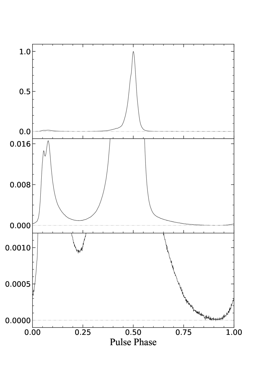
Figure 2: The averaged pulse profile of the whole bandwidth is shown in the top panel, and the corresponding $\times$60 and $\times$900 expanded scale views are plotted in the middle and bottom panels, respectively. The emission region of the pulse phase from 0.88 to 0.92 is regarded as the baseline region.

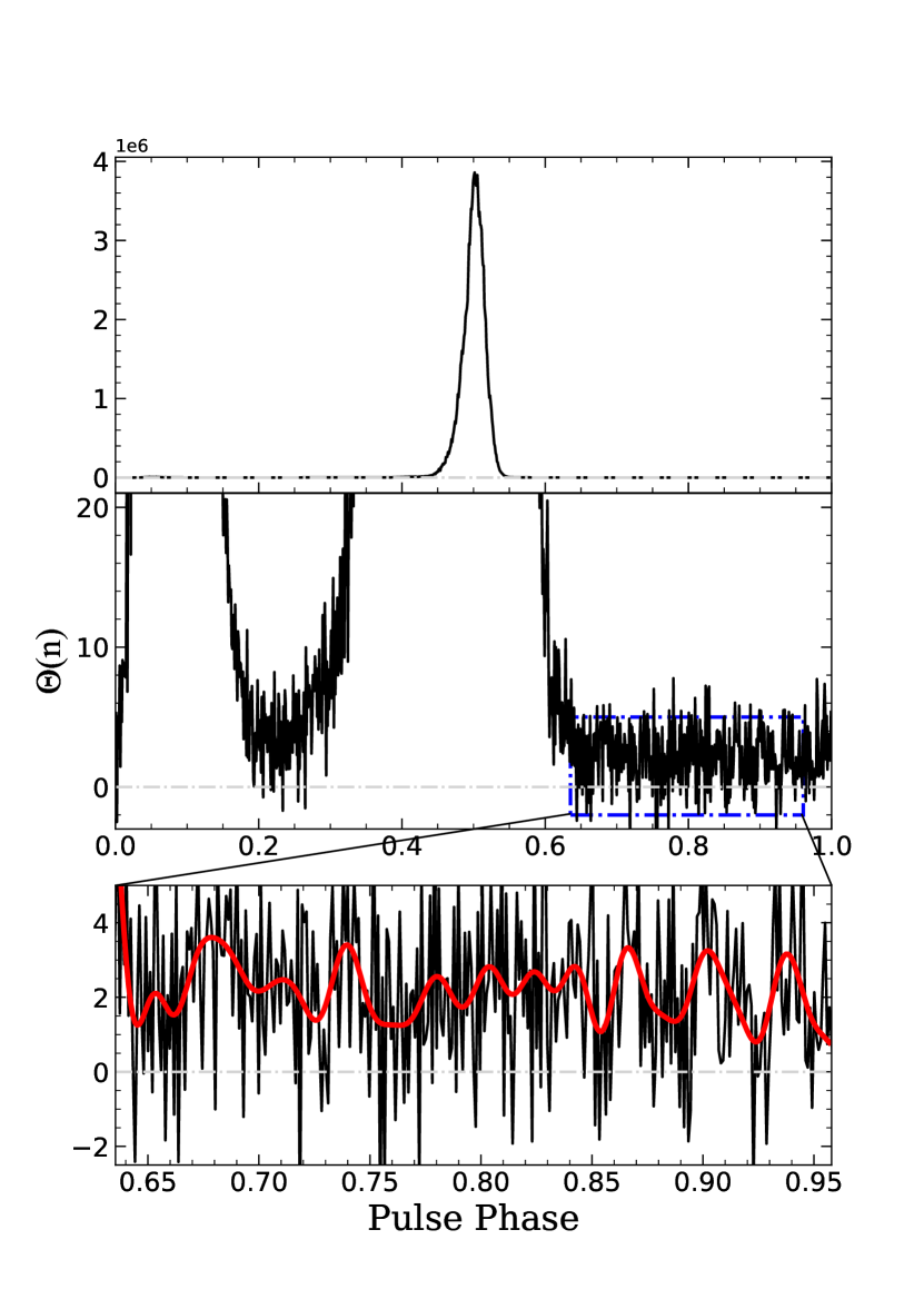
Figure 3: The $\Theta(n)$-function defined in equation (1) of the whole pulse longitude are shown in the top panel, and vertically zoomed-in view is plotted in the middle panel. Moreover, the detailed property of the blue region is zoomed in the bottom panel.

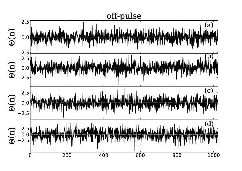
Figure 4: The behaviour of $\Theta(n)$-function for the simulated random data. Panels (a) and (b) correspond to gamma distributions with different shape parameters, and panels (c) and (d) represent log-normal and Gaussian distributions, respectively.

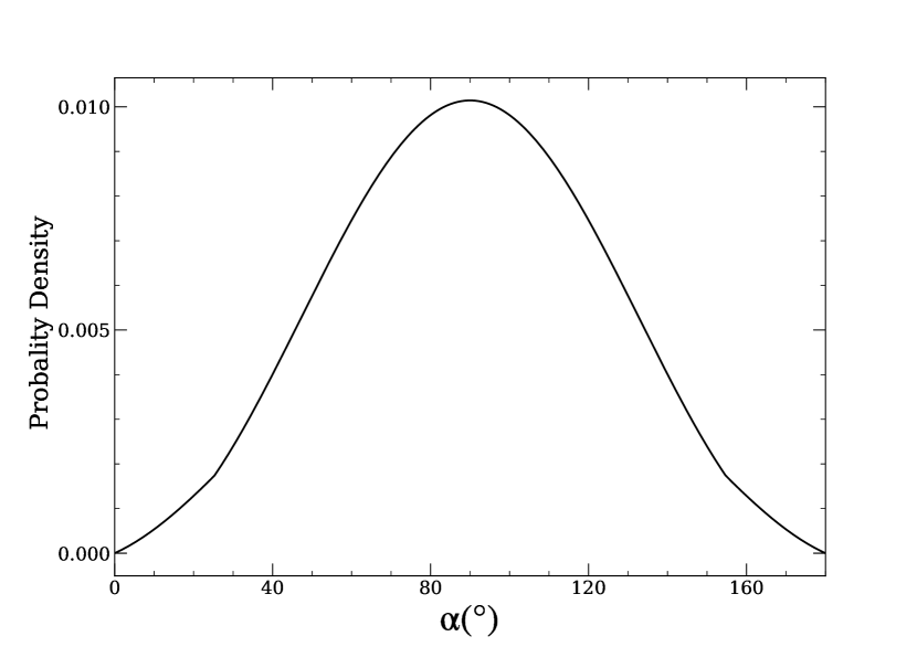
Figure 5: The probability density of magnetic inclination angle $\alpha$ derived from the period and pulse width of PSR B0950$+$08.

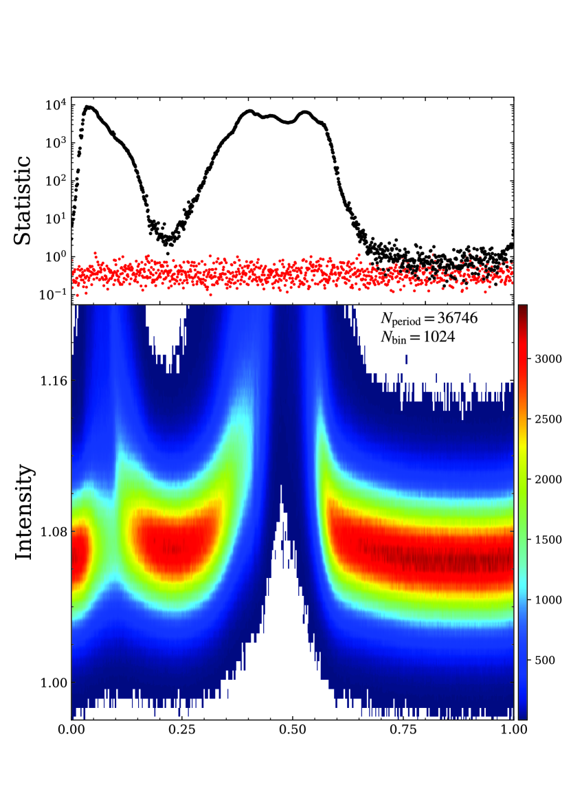
Figure 6: The radio signal distributions at each longitude are shown in the bottom panel, and the top panel shows the statistics of the Anderson-Darling test on them as the black points. The red points are the Anderson-Darling test statistics for the simulated random data with Gaussian distribution. And the number of single pulses with fixed radio emission intensity at each pulse phase is represented by different colors.

The $\Theta(n)$-function describes the statistical properties of the radio emission signal. The region of the on-pulse (the pulse longitudes which have periodic and impulsive emission) and off-pulse can be distinguished by this function, because the value of the $\Theta(n)$-function is positive at on-pulse regions and goes to zero at the off-pulse regions (see Appendix A). It should be noted that the fluctuation of the radio emission signals and noise may lead to the statistics error, and this error can possibly be eliminated if the number of the individual pulse ($N_{\mathrm{period}}$) is big enough. This statistical properties implies that the value of the $\Theta(n)$-function may be influenced by the background noise (discussed in Appendix B). A detailed behaviour of $\Theta(n)$-function at the entire pulse longitude is described as black curves in Fig. 3, and the detailed property of the blue region in the middle panel is zoomed in the bottom panel. From this figure, the result is obviously influenced by the background noise at the low-emission region. To determine the emission properties of these regions, the values of $\Theta(n)$-function at the low-emission region need to be smoothed. The red curve in the bottom panel is the smoothed result via low-pass filtering, and apparently, this curve at the low-emission region is greater than zero (dash-dot gray reference line). It is evident that, in the observed data, the values of the $\Theta(n)$-function at the two low-emission regions are positive. The behaviour of this function strongly illustrates that radio emission signals fill the low-emission region, and this result supports the whole phase radiation picture that the emission signals fill the entire $360^{\circ}$ pulse longitude. To better demonstrate that the $\Theta(n)$-function is equal to zero for continuous emission (the unpulsed emission) and is not affected by the non-linear instrumental response, and assuming that the non-linear instrumental response may cause the radio signals of each pulse phase to follow gamma or log-normal distribution, we simulate the $\Theta(n)$-function measurements for those distributions. The behavior of $\Theta(n)$-function for these simulations are shown in Fig. 4 to compare with the properties of $\Theta(n)$-function for the bridge emission region of PSR B0950$+$08. Panels (a), (b), (c) and (d) depict the gamma (with shape parameter of 3 and scale parameter of 1), gamma (with shape parameter of 5 and scale parameter of 1), log-normal (with shape parameter of 0.1 and scale parameter of 1) and Gaussian distribution, respectively, and the sample numbers of all simulated data are $10^{5}$. As these figures show, the values of the $\Theta(n)$-function are consistent with zero for continuous emission and the non-linear instrumental response.

4 conclusion and discussions

In this work, the impulsive emission characteristics of PSR B0950$+$08 are detected for the first time over the whole pulse phase. It is shown that the averaged pulse profile of this pulsar is consistent with previously presented works in the strong emission regions (e.g. McLaughlin & Rankin, 2004; Everett & Weisberg, 2001; Johnston et al., 2005). From Figs. 1,  2 and  3, it is evident that the emission of the low-emission region (from the pulse phase 0.65 to 0.95, the emission properties at this pulse longitude are undetected and usually regarded as off-pulse regions in published literature) have been detected for PSR B0950$+$08. With the detection of the emission at the bridge regions, the whole phase radiation characteristics of this pulsar are identified. However, there are some issues which need to be discussed.

The radio emission of the PSR B0950$+$08 may be originated from the two poles, which is different from the other whole-phase radiation pulsar, PSR B0826$-$34. Esamdin et al. (2005) reported that the radiation extends through the whole pulse phase of PSR B0826$-$34 in the “strong emission mode”. The radio emission signals of PSR B0826$-$34 covers the whole phase could naturally be understandable because the inclination angle, $\alpha$, is extremely low ($\sim 0.5^{\circ}$), as is evident from the large pulse width for this pulsar. Whereas, the pulse width of strong emission for PSR B0950$+$08 is relatively small ($\sim 31.4^{\circ}$), which implies a large inclination angle. With the assumption of the radiation altitude as 1000 km (at this altitude, the multi-pole field is weak and the field is dominated by the dipole component), one can calculate the maximum half width of the radiation beam, $\theta_{\mu}$ (corresponding to the radiation from the last open field lines), to be $\sim 25.8^{\circ}$. Assuming that the directions of the magnetic axis and rotation axis are uniform and ignore the beam scale distribution, with the Eq. 2 in Lee et al. (2009), we estimate the probability density of magnetic inclination angle, $\alpha$, which is shown in Fig. 5. It can be calculated that the probability density of the inclination angle (smaller that $10^{\circ}$ or larger than $170^{\circ}$) is $\sim 2.96\times 10^{-3}$. Moreover, the inclination angle measured through polarization observation of the strong emission is $\alpha\simeq 75^{\circ}$ (Everett & Weisberg, 2001), which implies the radiation of PSR B0950$+$08 originates from both poles of an almost orthogonal rotator. Therefore, the radio signals of the two bridge regions should be overlapped by radiation from the two poles.

The whole phase radiation implies that some radio emission from PSR B0950$+$08 must come from high altitude. However, the assumption of radiation altitude at 1000 km should be discussed carefully. In fact, the mean pulse profile at lower frequency is much wider, with pulse width $\sim 70^{\circ}$ (Bilous et al., 2022), which leads to that the radiation altitude must be higher than 1500 km under the assumption of $\alpha\simeq 75^{\circ}$. Furthermore, for the whole phase radiation, the maximum radiation altitude should be larger than 5000 km even after the adjustment for the effects of aberration and retardation. Considering the radius of the light cylinder for PSR B0950$+$08 of $\sim 12000$ km and its whole phase radiation characteristics, there must be a certain pulse longitude that the emission comes from the two poles at the same time, and it can be derived that the half width of at least one radiation beam, $\theta_{\mu}$, must not be less than $90^{\circ}$. According to the radiation altitude equation (see Eq.(5) in  Zhang et al. (2007)), it is calculated that the emission height of a certain pulse longitude (probably in the two low-emission regions) is larger than $\sim 8000$ km. With the inclination angle is $75^{\circ}$, it can be also calculated, at least 40% of the entire pulse period, the radiation comes from an extremely high altitude of 5000 km, which is roughly the altitude of the outer gap where the high energy emission is thought to be originated (Cheng et al., 1986). However, for the radio radiation of normal pulsars, the radiative particles are supposed to lose energy rapidly and not to keep radiating till reaching such a high altitude (Zhang et al., 1997). The radio emission is always regarded as being generated from low altitude of pulsars, due to two effects of the energy loss and the decoherence of the radiative particles which moving outwards along the opening magnetic field lines. The radiation altitude larger that 8000 km challenge the conventional particle acceleration and coherent radiation mechanism in pulsar magnetosphere discussed in Ruderman & Sutherland (1975), which may imply additional acceleration electric field over the polar gap, i.e., the slot gap (Arons, 1983) or annular gap (Qiao et al., 2007).

The whole pulse radiation characteristics is unveiled with the $\Theta(n)$-function, which exploits the variation property of the pulsar radiation. In other words, the invariant radiation does not affect the analysis results. For example, the stable emission from pulsar wind nebula which contributes off-pulse emission (Ruan et al., 2020) is different from the whole phase radiation from pulsar. In fact, the whole phase radiation is similar to the non-100% pulsed fraction radiation of the high energy pulsar, in which the emission occurs over the whole phase while some specific phase regions are preferred.

The physical origin of the radio emission at different pulse longitudes is also noteworthy. The averaged pulse profile shows complex shapes, and its radio emission beam is described by the so-called “core-cone” model. According to this model, the radio radiation beam consists of a central core surrounded by two rings of nested conal emission, which are respectively named the inner and outer cones (Rankin, 1983, 1990). Although the whole pulse longitude exhibits radio emission, the emission properties vary with different pulse longitudes. In Fig. 2 it can be seen that the well-resolved conal-double structure of the inter-pulse differs from the unresolved conal-single structure of main pulse. In Fig. 3, the values of $\Theta(n)$-function in the two low-emission regions are almost equal to each other, which may indicate similar emission physics.

To determine the emission properties of the bridge regions, the distribution of the radio emission signals at certain pulse longitude is also considered. This method reveal the emission properties through the distribution of the noise and radio emission at each pulse phase bin of the folded data, which follow different statistical laws. Apparently, the fluctuation of the noise follows the Gaussian distribution, and this statistical property is different with the log-normal distribution of the radio emission signals of the normal pulse (Cairns et al., 2001). This property may cause that the distribution of the emission at the on-pulse phase interval is asymmetric. The statistical results are shown in the bottom panel of Fig. 6, and the number of single pulses with fixed radio emission intensity at each pulse phase is represented by different colors. From this figure, it faintly shows that the distribution of the upper and lower of the maximum distribution point (the red points) at each pulse phase bin is asymmetric. To better illustrate the asymmetry of the whole pulse longitudes, a longitude-resolved test statistics such as Anderson-Darling test is also used with the null hypothesis that the distribution of each longitude comes from Gaussian distribution (Stephens, 1974). The Anderson-Darling statistics are shown in the top panel of Fig. 6 as black points, and the red points represent the results, which are derived from the simulated random data with Gaussian distribution. It demonstrates that the distribution at each longitude deviates the Gaussian distribution, which is consistent with the distribution characteristics in the bottom panel. Although it seems that the above method can also reveal the emission in the bridge regions, the flux distribution at each phase bin may be affected by weak RFI in frequency domain and non-linear response of the instrument. In contrast, the $\Theta(n)$-function would be better since that it just refers to the radiation variation characteristics in time domain.

Beside the method used above, the auto-correlation function (ACF) is widely used to reveal the structure characteristics of sub-pulse and micro-structure (Cordes, 1976). In this method, it is needed to use several phase bins (the number of phase bin is usually larger than 10) in each single pulse to calculate the ACF result, and then the conclusion about the radiation existence on the phase interval of these bins can be drawn. However, it is hard to distinguish if the radiation exists on a specific pulse phase due to the relatively long data length to calculate the ACF results. In addition, the ACF may also be influenced by other correlations in the recorded data, i.e., the correlation introduced by the dedispersion process and the red component of the system noise. In this paper, the $\Theta(n)$-function is introduced as method to judge the existence of the radiation at each phase bin. To calculate $\Theta(n)$-function, the correlation of the intensity evolution (instead of the intensity) between adjacent phase bins is obtained to show the impulsive property of sub-pulse. Therefore, the $\Theta(n)$-function represent the intensity correlation of the first order (while the classical ACF method reveal the zero order), which make it to avoid being influenced by the inaccuracy of the baseline. In addition, the longitude-longitude cross correlation can also be used to determine the sub-pulse width (Karastergiou et al., 2001). However, this method is strongly influenced by the accuracy of the baseline in each single pulse and would lose efficacy for the weak emission of PSR B0950$+$08.

In this work, the two low-emission regions of the averaged pulse profile for PSR B0950$+$08 exhibit significant concave structure rather that flat platform, which indicates that there is an impulsive radio emission at these two low-emission regions. A $\Theta(n)$-function is proposed to quantitatively determine the radio signal of the weak emission regions, classifying an impulsive. Through data analysis, the $\Theta(n)$-function is found to be a tentative method to determine the radio emission of the bridge regions for this pulsar, because it is just based on the emission correlation of any three adjacent phase bins. However, it would be noted that given the time-scale discussed in Appendix A, the $\Theta(n)$-function may not be suitable for detecting the radiation of all pulsars. It should be caution that if one applies the $\Theta(n)$-function to determine the radio signal in the weak emission regions for other pulsars.

It is difficult to determine the baseline position of PSR B0950$+$08, because the baseline determination for this pulsar is affected by many problems. For instance, the conventional baseline subtraction is not suitable for this pulsar. Secondly, the change of the baseline with time will affect its determination. Moreover, the radiation intensity of this pulsar is influenced by the effect of the interstellar scintillation (e.g. Bilous et al., 2022), which could also influence determining process. In fact, the baseline emission is much more difficult to remove completely for the single-dish radio telescope. In this work, the detection result of the $\Theta(n)$-function is hardly affected by the baseline emission of PSR B0950$+$08 for this observation, since it only depends on the pulsed radio signal of the sub-pulse of this pulsar. The baseline emission of the pulsar can be determined by the radio interferometer through analysing the spatial variation of the background emission. More precise measurements for the baseline emission of this pulsar may be provided by the future interferometers such as the SKA (Carilli, 2015) or the FAST extension array (FASTA).

The determination of the accuracy baseline is very important for the pulsar with the detectable emission over the whole pulse phase, since the PPA is related to the radiation geometry. But the PPA of the whole phase radiation is hard to be calibrated because it is sensitive to the baseline determination in the weak radiation phase region. The polarization features of this pulsar are not presented in this paper, since we have not made satisfied calibration during the observations. The non-linear evolution of baseline response with time severely influenced the calibration. Therefore, real time calibration information is needed to determine the baselines of the Stokes parameters precisely, and the optimized calibration of this pulsar has already been planned.

The effects of saturation from the digitization process, as presented in Jenet & Anderson (1998). There would be an artifact caused by the analog-to-digital conversion and dispersion, which may bring a scattered power into the data. This effect will result in a fake correlation along pulse phase and a wider radiation phase, and the range of this effect depends on the dispersion. It could be calculated that the dispersion sweep in our frequency range of 1050-1450 MHz is 5.3 ms, $\sim 2\%$ of the entire pulse period for PSR B0950$+$08. Thus, with the digitization effect, the radio pulse would be widened by 2% and an artificial correlation within 2% pulse period would be produced. The non-zero value of the $\Theta(n)$-function may be also induced by the time correlation. We expect that future interferometers such as the SKA or the FASTA will verify the current findings. Additionally, we anticipate that FAST and these future interferometers are potentially detecting more pulsars with whole phase radiation in the future.

Data Availability

The data underlying this work are available in the FAST project PT2020$-$0034, and can be shared on request to the FAST Data Center.

Appendix A the property of the $\Theta$-function

Detailed expression of the $\Theta(n)$-function is shown as equation(1), and here we will present that the values of $\Theta(n)$-function at the emission regions are positive.

For the data, at any pulse phase interval with emission, the intensity of the noise follows the Gaussian distribution. The properties of $\Theta(n)$-function can be described by the follows,

$$\begin{split}&\Theta(n)=\sum_{k=1}^{N_{\mathrm{period}}}\bigg{\{}2\left(I_{k,n-1}-I_{k,n+1}\right)^{2}\\ &-\left[\left(I_{k,n-1}-I_{k,n}\right)^{2}+\left(I_{k,n}-I_{k,n+1}\right)^{2}\right]\bigg{\}}\\ &=\sum_{k=1}^{N_{\mathrm{period}}}\bigg{\{}2\left(S_{k,n-1}-S_{k,n+1}+\sigma_{k,n-1}-\sigma_{k,n+1}\right)^{2}\\ &-\left[\left(S_{k,n-1}-S_{k,n}+\sigma_{k,n-1}-\sigma_{k,n}\right)^{2}\right]\\ &-\left[\left(S_{k,n+1}-S_{k,n}+\sigma_{k,n+1}-\sigma_{k,n}\right)^{2}\right]\bigg{\}}\\ &\approx\sum_{k=1}^{N_{\mathrm{period}}}\bigg{\{}2\left(S_{k,n-1}-S_{k,n+1}\right)^{2}-\\ &\left[\left(S_{k,n-1}-S_{k,n}\right)^{2}+\left(S_{k,n}-S_{k,n+1}\right)^{2}\right]\bigg{\}},\end{split}$$ (2)

where $S_{k,n}$ and $\sigma_{k,n}$ are the emission signal and noise intensity contributed by the $k$-th pulse and $n$-th pulse phase bin,respectively.

For the observation data, a same structure of the sub-pulse repeat many times in a large number of cycles, so that a pulse phase is ergodic in all positions of sub-pulse. In other words, the summation of all cycles is equivalent to that of all points in sub-pulses with different shape,

$$\begin{split}&\Theta(n)\approx\sum_{k=1}^{N_{\mathrm{period}}}\frac{1}{L}\sum_{l=1}^{L}\bigg{\{}2\left(S_{k,n,l-1}-S_{k,n,l+1}\right)^{2}\\ &-\left[\left(S_{k,n,l}-S_{k,n,l-1}\right)^{2}+\left(S_{k,n,l}-S_{k,n,l+1}\right)^{2}\right]\bigg{\}}\\ &\approx\sum_{k=1}^{N_{\mathrm{period}}}\frac{1}{L}\sum_{l=1}^{L}\bigg{\{}\left(S_{k,n,l}-S_{k,n,l-1}\right)^{2}+\left(S_{k,n,l+1}-S_{k,n,l}\right)^{2}\\ &+4\left(S_{k,n,l}-S_{k,n,l-1}\right)\left(S_{k,n,l+1}-S_{k,n,l}\right)\bigg{\}}\\ &\approx\sum_{k=1}^{N_{\mathrm{period}}}\frac{1}{L}\sum_{l=1}^{L}\left(\Delta_{l}^{2}+\Delta^{2}_{l-1}+4\Delta_{l}\Delta_{l-1}\right)\end{split}$$ (3)

where $S_{k,n,l}$ is the $l$-th bin of the sub-pulse with $L$ bins of the $k$-th pulse and $n$-th pulse phase bin, $\Delta_{l}=S_{k,n,l+1}-S_{k,n,l}$ is the first order difference of the sub-pulse.

In this work, the time resolution of the folded data is $\sim$0.25 ms. According to the previous work, the characteristics time-scale of the fine structure is $\sim$1 ms for PSR B0950$+$08 (Ulyanov et al., 2016). In other words, the second order difference can hardly change sign in succession in 1 ms ($\sim$4 phase bins) for the folded data. In the interval that the second order difference has same sign (the bin index of the start and end of the interval are $l_{\mathrm{s}}$ and $l_{\mathrm{e}}$,respectively), $\Delta_{l}$ is monotonic. Fig. 7 shows an example of the profile shape and its differences at first and second order in the top, middle and bottom panels, respectively, and the vertical dot-dashed lines in the figure divide the profile into several segments. It can be seen that second order difference in each segment has same sign, and the first order difference is monotonic. If the sign of $\Delta_{l}$ does not change, we have $M=\displaystyle\sum_{l=l_{\mathrm{s}}}^{l_{\mathrm{e}}}\left(\Delta_{l}^{2}+\Delta^{2}_{l-1}+4\Delta_{l}\Delta_{l-1}\right)\geq 0$. Otherwise, if $\Delta_{l}$ changes signs, without loss of generality, suppose $\Delta_{l_{\mathrm{s}}}\geq...\geq\Delta_{m}>0\geq\Delta_{m+1}\geq...\geq\Delta_{l_{\mathrm{e}}}$, it follows that

$$\begin{split}&\sum_{l_{\mathrm{s}}}^{l_{\mathrm{e}}}\left(\Delta_{l}^{2}+\Delta^{2}_{l-1}+4\Delta_{l}\Delta_{l-1}\right)\\ &=\sum_{l=m-1}^{l_{\mathrm{s}}}\left(\Delta_{l}^{2}+\Delta^{2}_{l-1}+4\Delta_{l}\Delta_{l-1}\right)+\left(\Delta_{m}^{2}+\Delta^{2}_{m-1}+4\Delta_{m}\Delta_{m-1}\right)\\ &+\left(\Delta_{m+1}^{2}+\Delta^{2}_{m}+4\Delta_{m+1}\Delta_{m}\right)+\sum_{l=m+2}^{l_{\mathrm{e}}}\left(\Delta_{l}^{2}+\Delta^{2}_{l-1}+4\Delta_{l}\Delta_{l-1}\right)\\ &\geq\left(\Delta_{m}^{2}+\Delta^{2}_{m-1}+4\Delta_{m}\Delta_{m-1}\right)+\left(\Delta_{m+1}^{2}+\Delta^{2}_{m}+4\Delta_{m+1}\Delta_{m}\right)\\ &=\Delta_{m-1}^{2}-2\Delta_{m}^{2}+4\Delta_{m}\Delta_{m-1}+(\Delta_{m+1}+2\Delta_{m})^{2}\\ &\geq\Delta_{m-1}^{2}-2\Delta_{m}^{2}+4\Delta_{m}\Delta_{m-1}\\ &\geq\Delta_{m}^{2}-2\Delta_{m}^{2}+4\Delta_{m}^{2}\\ &=3\Delta_{m}^{2}>0.\end{split}$$ (4)

To sum up, $\Theta(n)>0$ at the interval of the emission pulse phase.

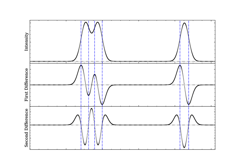
Figure 7: Intensity profile shape and its differences, and the dot-dashed gray line represents the reference zero line. The vertical dot-dashed lines divide the profile into several segments based on the sign of the second order difference.

Appendix B The effects of the background noise

When using the $\Theta(n)$-function to quantitatively determine the emission characteristics of the weak regions, such as the two low-emission regions of PSR B0950$+$08 in this work, one concern is the effects of the background noise. particularly the red noise components. Fig. 8 shows the spectrum of the background noise intensity relative to the white noise, and red line corresponds to the power-law fitting of the red noise component, $P(f)=3.969\times 10^{-3}f^{-1.506}$. With the power-law expression, the background noise is simulated, which has same white noise intensity as the observed data. The simulated red noise is shown in Fig. 9. The values of the $\Theta(n)$-function of the simulated noise is calculated, which is presented in the panel (a) of the Fig. 10. In addition, for comparison, the $\Theta(n)$-function of the pure red noise component is shown in the panel (b). It can be seen that the positive property of the $\Theta(n)$-function is hardly affected by the red noise components in this observation, and the fluctuations of the $\Theta(n)$-function in Fig. 3 are almost resulted from the background noise.

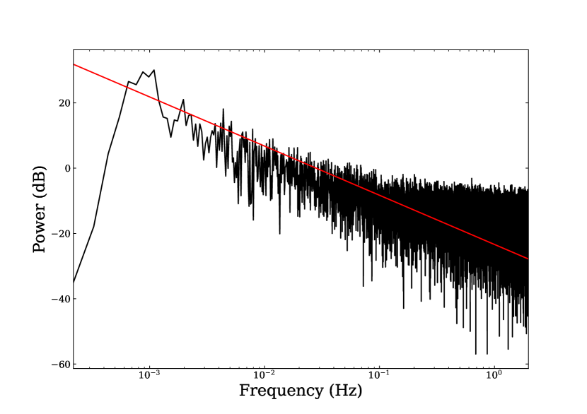
Figure 8: The spectrum of the background noise intensity is normalized by its white noise intensity, and the red line corresponds to the power-law fitting. The background noise intensity is obtained by averaging the minimum 10 phase bins in each period.

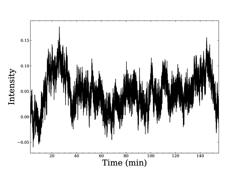
Figure 9: Simulated noise according to the power-law of $P(f)=3.969\times 10^{-3}f^{-1.506}$, and it has same the white noise intensity as the background noise.

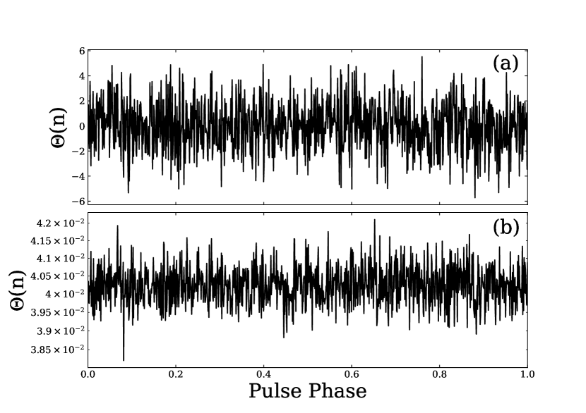
Figure 10: The $\Theta(n)$-function of the simulated background noise and its red noise components are shown in panels (a) and (b), respectively.

References

- Arons (1983) Arons J., 1983, ApJ, 266, 215
- Bilous et al. (2022) Bilous A. V., et al., 2022, A&A, 658, A143
- Cairns (2004) Cairns I. H., 2004, ApJ, 610, 948
- Cairns et al. (2001) Cairns I. H., Johnston S., Das P., 2001, ApJ, 563, L65
- Carilli (2015) Carilli C., 2015, in Advancing Astrophysics with the Square Kilometre Array (AASKA14). p. 171 (arXiv:1408.5317)
- Cheng et al. (1986) Cheng K. S., Ho C., Ruderman M., 1986, ApJ, 300, 500
- Cordes (1976) Cordes J. M., 1976, ApJ, 208, 944
- Dai et al. (2015) Dai S., et al., 2015, MNRAS, 449, 3223
- Esamdin et al. (2005) Esamdin A., Lyne A. G., Graham-Smith F., Kramer M., Manchester R. N., Wu X., 2005, MNRAS, 356, 59
- Everett & Weisberg (2001) Everett J. E., Weisberg J. M., 2001, ApJ, 553, 341
- Hankins & Cordes (1981) Hankins T. H., Cordes J. M., 1981, ApJ, 249, 241
- Hankins et al. (1991) Hankins T. H., Izvekova V. A., Malofeev V. M., Rankin J. M., Shitov Y. P., Stinebring D. R., 1991, ApJ, 373, L17
- Hobbs et al. (2004) Hobbs G., Lyne A. G., Kramer M., Martin C. E., Jordan C., 2004, MNRAS, 353, 1311
- Hotan et al. (2004) Hotan A. W., van Straten W., Manchester R. N., 2004, Publ. Astron. Soc. Australia, 21, 302
- Jenet & Anderson (1998) Jenet F. A., Anderson S. B., 1998, PASP, 110, 1467
- Jiang et al. (2019) Jiang P., et al., 2019, Science China Physics, Mechanics, and Astronomy, 62, 959502
- Jiang et al. (2020) Jiang P., et al., 2020, Research in Astronomy and Astrophysics, 20, 064
- Johnston et al. (2005) Johnston S., Hobbs G., Vigeland S., Kramer M., Weisberg J. M., Lyne A. G., 2005, MNRAS, 364, 1397
- Karastergiou et al. (2001) Karastergiou A., et al., 2001, A&A, 379, 270
- Kuzmin et al. (1998) Kuzmin A. D., Izvekova V. A., Shitov Y. P., Sieber W., Jessner A., Wielebinski R., Lyne A. G., Smith F. G., 1998, A&AS, 127, 355
- Lee et al. (2009) Lee K. J., Cui X. H., Wang H. G., Qiao G. J., Xu R. X., 2009, ApJ, 703, 507
- Lu et al. (2019) Lu J., et al., 2019, Science China Physics, Mechanics, and Astronomy, 62, 959505
- Marcote et al. (2019) Marcote B., Maan Y., Paragi Z., Keimpema A., 2019, A&A, 627, L2
- McLaughlin & Rankin (2004) McLaughlin M. A., Rankin J. M., 2004, MNRAS, 351, 808
- Navarro et al. (1995) Navarro J., de Bruyn A. G., Frail D. A., Kulkarni S. R., Lyne A. G., 1995, ApJ, 455, L55
- Nowakowski et al. (2002) Nowakowski L. A., Bhat N. D. R., Lorimer D. R., 2002, in American Astronomical Society Meeting Abstracts. p. 118.02
- Popov et al. (2002) Popov M. V., Bartel N., Cannon W. H., Novikov A. Y., Kondratiev V. I., Altunin V. I., 2002, A&A, 396, 171
- Qiao et al. (2007) Qiao G.-J., Lee K.-J., Zhang B., Wang H.-G., Xu R.-X., 2007, Chinese J. Astron. Astrophys., 7, 496
- Radhakrishnan & Cooke (1969) Radhakrishnan V., Cooke D. J., 1969, Astrophys. Lett., 3, 225
- Rankin (1983) Rankin J. M., 1983, ApJ, 274, 333
- Rankin (1990) Rankin J. M., 1990, ApJ, 352, 247
- Ruan et al. (2020) Ruan D., Taylor G. B., Dowell J., Stovall K., Schinzel F. K., Demorest P. B., 2020, MNRAS, 495, 2125
- Ruderman & Sutherland (1975) Ruderman M. A., Sutherland P. G., 1975, ApJ, 196, 51
- Shabanova & Shitov (2004) Shabanova T. V., Shitov Y. P., 2004, A&A, 418, 203
- Singal & Vats (2012) Singal A. K., Vats H. O., 2012, AJ, 144, 155
- Stephens (1974) Stephens M. A., 1974, Journal of the American Statistical Association, 69, 730
- Tsai et al. (2015) Tsai J.-W., et al., 2015, AJ, 149, 65
- Ulyanov et al. (2016) Ulyanov O. M., Skoryk A. O., Shevtsova A. I., Plakhov M. S., Ulyanova O. O., 2016, MNRAS, 455, 150
- Xu (2021) Xu R., 2021, National Science Review, 8, nwab204
- Zhang et al. (1997) Zhang B., Qiao G. J., Han J. L., 1997, ApJ, 491, 891
- Zhang et al. (2007) Zhang H., Qiao G. J., Han J. L., Lee K. J., Wang H. G., 2007, A&A, 465, 525
- van Straten & Bailes (2011) van Straten W., Bailes M., 2011, Publ. Astron. Soc. Australia, 28, 1