Noncolliding Macdonald Walks with an Absorbing Wall

Noncolliding Macdonald Walks
with an Absorbing Wall

Leonid PETROV

L. Petrov

University of Virginia, Charlottesville, VA, USA lenia.petrov@gmail.com https://lpetrov.cc/

Received June 07, 2022, in final form October 16, 2022; Published online October 20, 2022

The branching rule is one of the most fundamental properties of the Macdonald symmetric polynomials. It expresses a Macdonald polynomial as a nonnegative linear combination of Macdonald polynomials with smaller number of variables. Taking a limit of the branching rule under the principal specialization when the number of variables goes to infinity, we obtain a Markov chain of $m$ noncolliding particles with negative drift and an absorbing wall at zero. The chain depends on the Macdonald parameters $(q,t)$ and may be viewed as a discrete deformation of the Dyson Brownian motion. The trajectory of the Markov chain is equivalent to a certain Gibbs ensemble of plane partitions with an arbitrary cascade front wall. In the Jack limit $t=q^{\beta/2}\to 1$ the absorbing wall disappears, and the Macdonald noncolliding walks turn into the $\beta$-noncolliding random walks studied by Huang [Int. Math. Res. Not. 2021 (2021), 5898–5942, arXiv:1708.07115]. Taking $q=0$ (Hall–Littlewood degeneration) and further sending $t\to 1$, we obtain a continuous time particle system on $\mathbb{Z}_{\geq 0}$ with inhomogeneous jump rates and absorbing wall at zero.

Macdonald polynomials; branching rule; noncolliding random walks; lozenge tilings

06C05; 05E05; 05A30

1 Introduction

1.1 Overview

The Dyson Brownian motion [8] is a continuous stochastic dynamics of $N$ particles on the one-dimensional line $\mathbb{R}$. The particles evolve according to independent Brownian motions which are conditioned to never collide. The noncolliding property may be also modeled as Coulomb repelling. The Dyson Brownian motion arises as the dynamics of eigenvalues from the standard Brownian motion on the space of complex Hermitian matrices. As such, it has been heavily utilized towards universality results for random matrix spectra [1, 9, 14].

Within integrable probability, a number of discrete deformations of the Dyson Brownian motion were introduced, starting from noncolliding Poisson and Bernoulli random walks [19] (based on a classical formula of [16]) and followed by their Macdonald deformation depending on two parameters $(q,t)$ which is defined in [3]. A notable special case of the latter considered in [12] is the Jack limit $t=q^{\beta/2}\to 1$, where $\beta>0$ is the beta parameter from random matrix theory. In the Jack limit, one obtains $\beta$-noncolliding Poisson random walks (further studied in [13]), and also their multilevel versions. A scaling limit of the latter leads to the multilevel Dyson Brownian motion with the general $\beta$ parameter.

Each of the known discrete deformations of the Dyson Brownian motion is powered by the Cauchy summation identity for some family of symmetric polynomials $\left\{P_{\lambda}\right\}$ such as Schur (for noncolliding Poisson and Bernoulli walks), Jack, or Macdonald polynomials. Here $\left\{P_{\lambda}\right\}$ is one of these families of polynomials in $N$ variables. The $P_{\lambda}$’s form a linear basis in the space of symmetric polynomials in $N$ variables as $\lambda$ runs over partitions $\lambda=(\lambda_{1}\geq\dots\geq\lambda_{N}\geq 0)$, $\lambda_{i}\in\mathbb{Z}$, with $N$ parts.

The Cauchy identity is a fundamental property of many families of symmetric polynomials, and is closely tied to their orthogonality with respect to a suitable inner product. It provides a product-form expression for the sum $\sum_{\lambda}b_{\lambda}P_{\lambda}(x_{1},\dots,x_{N})P_{\lambda}(y_{1},\dots,y_{N})$, where $b_{\lambda}$ are certain explicit coefficients. In stochastic dynamics of $N$ noncolliding particles, this Cauchy identity implies the normalization to one property of the transition probability, which also involves an $N$-fold summation over partitions $\lambda$.

Along with the Cauchy identity, most families of symmetric polynomials satisfy a branching rule. This identity expresses $P_{\lambda}(x_{1},\dots,x_{N})$ in $N$ variables as a nonnegative linear combination of polynomials $P_{\mu}(x_{1},\dots,x_{N-1})$ with $N-1$ variables, where the sum runs over $\mu$. For particular symmetric polynomials, such an expansion has clear representation-theoretic meaning. For example, for Schur polynomials the branching rule is behind the decomposition of a given irreducible representation of the unitary group $U(N)$ when restricted to the subgroup $U(N-1)$.

Note that the branching rule is often dual to the Pieri rule expressing the product $f\hskip 1.0ptP_{\lambda}$ (for a special choice of $f$ like $x_{1}+\dots+x_{N}$) as a linear combination of $P_{\nu}$’s in the same number of variables. In the present paper we do not explicitly use this duality, and keep the branching rule perspective.

The goal of the present work is to construct and explore noncolliding random walks arising from the branching rule instead of the Cauchy identity. We start at the level of Macdonald polynomials with parameters $(q,t)\in(0,1)^{2}$, and take a limit of the branching rule under the principal specialization $(x_{1},\dots,x_{N})=\big{(}1,t,\dots,t^{N-1}\big{)}$ as the number of variables $N$ goes to infinity. Using the resulting summation identity (formulated in Theorem 1.1 later in the introduction), we define a new discrete-time Markov process $\Upsilon_{m}$ of $m$ distinct ordered particles in $\mathbb{Z}_{\geq 0}$ with negative drift and absorbing wall at zero (where $m\in\mathbb{Z}_{\geq 1}$ is assumed fixed). The presence of the wall means that the process almost surely reaches its only absorbing state $(m-1,m-2,\dots,2,1,0)$.

Trajectories of $\Upsilon_{m}$ may be identified with lozenge tilings or plane partitions with certain explicit boundary conditions depending on the initial configuration in $\Upsilon_{m}$. We show that the probability measure on plane partitions coming from $\Upsilon_{m}$ has a Gibbs characterization via the so-called Boltzmann factors which are ratios of probability weights of two configurations differing by an elementary transformation. We explicitly compute these Boltzmann factors in the general Macdonald case. In the particular case $t=q$, the Gibbs probability weight of a plane partition is proportional simply to $q^{\mathsf{vol}}$, where $\mathsf{vol}$ is the sum of the entries of the plane partition. See Section 5 in the text for details.

We consider a number of degenerations of our process $\Upsilon_{m}$ leading to known deformations of the Dyson Brownian motion mentioned above. All these degenerations correspond to specializing the parameters $(q,t)$ in such a way that the Macdonald polynomials turn into another well-known family of symmetric polynomials:

• (Schur polynomials) Setting $t=q$, we get a simpler Markov process $\Upsilon_{m}^{\mathrm{Schur}}$ of $m$ noncolliding particles on $\mathbb{Z}_{\geq 0}$ with an absorbing wall at $0$. To the best of the author’s knowledge, this process and the underlying normalization identity (stating that the quantities in (4.1) below sum to $1$) are also new. The process $\Upsilon_{m}^{\mathrm{Schur}}$ looks similar to the translation invariant $q$-noncolliding random walks on $\mathbb{Z}$ introduced and studied in [5]. The normalization of transition probabilities in the latter process can be traced back to the Cauchy identity. However, it does not seem that our process $\Upsilon_{m}^{\mathrm{Schur}}$ can be scaled to that of [5].

• (Jack polynomials) Take $t=q^{\beta/2}\to 1$ (where $\beta>0$ is the parameter coming from random matrix theory), and simultaneously scale the coordinates of the process $\Upsilon_{m}$ away from $0$. In this way we get a dynamics of $m$ particles on $\mathbb{Z}$ which is invariant under space translations of the particles. This dynamics is closely related to the $\beta$-noncolliding Poisson random walks studied in [12, 13]. Thus, we see that our new Macdonald noncolliding walks $\Upsilon_{m}$ generalize all known noncolliding processes at the Jack level (with general random matrix $\beta$ parameter). In the particular case $\beta=2$, we recover the Bernoulli and Poisson walks conditioned to never collide which were studied in [19]. Under Brownian scaling, it is known that the latter random walks turn into the classical Dyson Brownian motion coming from Hermitian random matrices.

• (Hall–Littlewood polynomials) Setting $q=0$, further sending $t\to 1$ and taking a Poisson-type limit from discrete time to continuous, we arrive at a new particle system $\Upsilon_{m}^{\mathrm{cont}}$ on $\mathbb{Z}_{\geq 0}$ with an absorbing wall at zero which evolves as follows. To each particle $\mathsf{x}_{1}>\dots>\mathsf{x}_{m}\geq 0$ we assign an independent exponential clock of rate $i(\mathsf{x}_{i}-\mathsf{x}_{i+1}-1)$, where, by agreement, $\mathsf{x}_{m+1}=-1$. When the clock of $\mathsf{x}_{i}$ rings, we additionally select an index $j\in\{1,\dots,i\}$ uniformly at random, and all the particles $\mathsf{x}_{i},\mathsf{x}_{i-1},\dots,\mathsf{x}_{j}$ simultaneously jump to the left by $1$. The process $\Upsilon_{m}^{\mathrm{cont}}$ almost surely reaches its absorbing state $(m-1,\dots,1,0)$. A more detailed investigation of this particle system will be performed elsewhere.

In the next Section 1.2 we describe in detail our most general Markov processes $\Upsilon_{m}$ arising at the Macdonald level.

1.2 Macdonald noncolliding walks

Throughout the paper we assume that $(q,t)$ are real numbers belonging to $(0,1)$. We need some notation. Recall that the $q$-Pochhammer symbols are given by

$$(z;q)_{k}\coloneqq(1-z)(1-zq)\cdots\big{(}1-zq^{k-1}\big{)},\qquad k\in\mathbb{Z}_{\geq 0},$$

and $(z;q)_{\infty}\coloneqq\prod_{i=0}^{\infty}(1-zq^{i})$ is a convergent infinite product because $|q|<1$.

For $\vec{\mathsf{x}}=(\mathsf{x}_{1}>\dots>\mathsf{x}_{m}\geq 0)$, denote the $(t,q)$-deformed Vandermonde product by

$$V_{t,q}(\vec{\mathsf{x}}):=\prod_{1\leq i<j\leq m}\frac{\left(q^{j-i-1}t^{\mathsf{x}_{i}-\mathsf{x}_{j}-j+i+1};t\right)_{\infty}}{(q^{j-i}t^{\mathsf{x}_{i}-\mathsf{x}_{j}-j+i+1};t)_{\infty}}.$$ (1.1)

When $t=q\to 1$, $V_{t,q}$ turns (after rescaling by a suitable power of $\log q$) into the usual Vandermonde $V(\vec{\mathsf{x}})=\prod_{1\leq i<j\leq m}(\mathsf{x}_{i}-\mathsf{x}_{j})$. Moreover, when $\mathsf{x}_{i}=\mathsf{x}_{i+1}$ for some $i$, one readily sees that $V_{t,q}(\vec{\mathsf{x}})$ vanishes.

Let $\mathsf{y}=(\mathsf{y}_{1}>\dots>\mathsf{y}_{m}\geq 0)$ be such that

$$\mathsf{y}_{i}-\mathsf{x}_{i}\in\{-1,0\}\qquad\text{for all $1\leq i\leq m$}.$$ (1.2)

Now we can define the main object of the present paper:

$$\Upsilon_{m}(\vec{\mathsf{x}},\vec{\mathsf{y}})\coloneqq t^{-\binom{m}{2}}\hskip 1.0pt\frac{V_{t,q}(\vec{\mathsf{y}})}{V_{t,q}(\vec{\mathsf{x}})}\prod_{\begin{subarray}{c}1\leq i<j\leq m\\ \mathsf{y}_{i}=\mathsf{x}_{i},\,\mathsf{y}_{j}=\mathsf{x}_{j}-1\end{subarray}}\frac{\big{(}1-t^{i-j+\mathsf{x}_{i}-\mathsf{x}_{j}+1}q^{j-i-1}\big{)}\big{(}1-t^{i-j+\mathsf{x}_{i}-\mathsf{x}_{j}}q^{j-i+1}\big{)}}{\big{(}1-t^{i-j+\mathsf{x}_{i}-\mathsf{x}_{j}+1}q^{j-i}\big{)}\big{(}1-t^{i-j+\mathsf{x}_{i}-\mathsf{x}_{j}}q^{j-i}\big{)}}$$

$$\hphantom{\Upsilon_{m}(\vec{\mathsf{x}},\vec{\mathsf{y}})\coloneqq}{}\times\prod_{i\colon\mathsf{y}_{i}=\mathsf{x}_{i}}t^{\mathsf{x}_{i}}\prod_{i\colon\mathsf{y}_{i}=\mathsf{x}_{i}-1}\big{(}t^{m-i}-q^{m-i}t^{\mathsf{x}_{i}}\big{)}.$$ (1.3)

From (1.2) one readily sees that the infinite products in ${V_{t,q}(\vec{\mathsf{y}})}/{V_{t,q}(\vec{\mathsf{x}})}$ cancel out in such a way that (1.3) is always a rational function of $q$, $t$. Moreover, for $0<q,t<1$ the quantities (1.3) are nonnegative. One of our main results is the sum-to-one identity for the $\Upsilon_{m}$’s:

Theorem 1.1.

With the above notation, for any $\vec{\mathsf{x}}=(\mathsf{x}_{1}>\dots>\mathsf{x}_{m}\geq 0)$ we have

$$\sum_{\begin{subarray}{c}\vec{\mathsf{y}}=(\mathsf{y}_{1}>\dots>\mathsf{y}_{m}\geq 0)\\ \mathsf{y}_{i}-\mathsf{x}_{i}\in\left\{-1,0\right\}\ \text{for all $1\leq i\leq m$}\end{subarray}}\Upsilon_{m}(\vec{\mathsf{x}},\vec{\mathsf{y}})=1.$$

Theorem 1.1 implies that the quantities $\Upsilon_{m}(\vec{\mathsf{x}},\vec{\mathsf{y}})$ may be viewed as transition probabilities of a discrete time Markov chain of $m$ ordered distinct particles on $\mathbb{Z}_{\geq 0}$ in which at each step, each particle either stays, or moves to the left by $1$. Eventually with probability $1$ the chain reaches the absorbing state $(m-1,m-2,\dots,2,1,0)$, see Proposition 3.3 below. We call the Markov chain $\Upsilon_{m}$ the Macdonald noncolliding walks with an absorbing wall at zero.

We prove Theorem 1.1 in Section 3 by obtaining the transition probabilities $\Upsilon_{m}(\vec{\mathsf{x}},\vec{\mathsf{y}})$ as a limit of certain ratios of Macdonald polynomials evaluated at the principal specializations $\big{(}1,t,t^{2},\dots,t^{N-1}\big{)}$, as the number of variables goes to infinity. The fact that before the limit these ratios sum to one is equivalent to the branching rule for the Macdonald polynomials.

1.3 Outline

In Section 2 we review the definition of Macdonald symmetric polynomials together with all the required formulas. In Section 3 we perform the main limit transition, and obtain the Macdonald noncolliding walks $\Upsilon_{m}$. In Section 4 we consider various degenerations of our dynamics when the Macdonald parameters $(q,t)$ are specialized in a certain way. More precisely, we look at the dynamics at $t=q$ (when the Macdonald polynomials reduce to the Schur polynomials), as $q=t^{\alpha}\to 1$ (reduction to the Jack polynomials), and as $q=0$ (when Macdonald polynomials become the Hall–Littlewood polynomials). Moreover, in the latter case we see that sending $t\to 1$ leads to a new continuous time Markov chain on $m$ particles with inhomogeneous jump rates. In Section 5 we give a Gibbs characterization of the probability measure on the space of trajectories of our noncolliding walks by means of the so-called Boltzmann factors which are ratios of probability weights of two trajectories differing by an elementary transformation.

2 Review of Macdonald polynomials

Here we collect the necessary notation and results around Macdonald symmetric polynomials. We follow [20, Chapter VI].

2.1 Definition

Let $N\geq 1$. Macdonald symmetric polynomials $P_{\lambda}$ in $N$ variables $x_{1},\dots,x_{N}$ are indexed by partitions $\lambda=(\lambda_{1}\geq\dots\geq\lambda_{N}\geq 0)$, $\lambda_{i}\in\mathbb{Z}$, with $N$ parts. Denote the set of these partitions by $\mathbb{Y}(N)$. The $P_{\lambda}$’s depend on two parameters $q,t\in[0,1)$. For each fixed $(q,t)$, they form a basis in the space of symmetric polynomials in $N$ variables when $\lambda$ runs over $\mathbb{Y}(N)$. The shortest definition of the $P_{\lambda}$’s is through the first Macdonald $q$-difference operator acting in the $x_{i}$’s:

$$D_{1}\coloneqq\sum_{i=1}^{N}\biggl{(}\prod_{1\leq j\leq N\colon j\neq i}\frac{x_{j}-tx_{i}}{x_{j}-x_{i}}\biggr{)}T_{q;i},$$

$$T_{q;i}f(x_{1},\dots,x_{N})\coloneqq f(x_{1},\dots,x_{i-1},qx_{i},x_{i+1},\dots,x_{N}).$$

The operator $D_{1}$ preserves the space of symmetric polynomials in $x_{1},\dots,x_{N}$, and its eigenfunctions are the Macdonald polynomials

$$D_{1}P_{\lambda}(x_{1},\dots,x_{N}\mid q,t)=\bigl{(}q^{\lambda_{1}}t^{N-1}+q^{\lambda_{2}}t^{N-2}+\dots+q^{\lambda_{N}}\bigr{)}P_{\lambda}(x_{1},\dots,x_{N}\mid q,t),$$ (2.1)

with $\lambda\in\mathbb{Y}(N)$. For generic $(q,t)$, the eigenvalues in (2.1) for different $\lambda$ are distinct, so the $P_{\lambda}$’s are determined uniquely up to normalization. The normalization is specified by

$$P_{\lambda}(x_{1},\dots,x_{N}\mid q,t)=x_{1}^{\lambda_{1}}x_{2}^{\lambda_{2}}\cdots x_{N}^{\lambda_{N}}+\text{lexicographically lower terms},$$

where the lower terms depend on $q$, $t$.

In the case $q=t$, the polynomials $P_{\lambda}$ reduce to the well-known Schur symmetric polynomials $s_{\lambda}$, which admit the following explicit determinantal formula (which does not depend on the choice of $q$):

$$P_{\lambda}(x_{1},\dots,x_{N}\mid q,q)=s_{\lambda}(x_{1},\dots,x_{N})=\frac{\det\bigl{[}x_{i}^{\lambda_{j}+N-j}\bigr{]}_{i,j=1}^{N}}{\det\bigl{[}x_{i}^{N-j}\bigr{]}_{i,j=1}^{N}}.$$ (2.2)

For generic $(q,t)$, there are no known formulas for Macdonald polynomials which are as compact as (2.2).

2.2 Principal specialization

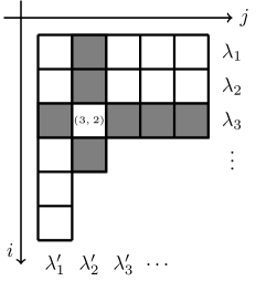
Figure 1: Young diagram $\lambda=(5,5,5,2,1,1)$. Highlighted are the arm, leg, coarm, and coleg of the box $\square=(3,2)$. We have $|\lambda|=19$ and $a(\square)=3$, $l(\square)=1$, $a^{\prime}(\square)=1$, $l^{\prime}(\square)=2$.

When the variables $x_{i}$ are specialized to a finite geometric progression with the ratio $t$ (the second Macdonald parameter), the polynomials $P_{\lambda}$ admit an explicit product formula in terms of the Young diagram corresponding to the partition $\lambda$. Recall that the Young diagram $\lambda$ is a collection of $1\times 1$ boxes in the plane with $\lambda_{i}$ boxes in row $i$, see Figure 1 for an illustration. The principal specialization takes the form [20, formulas (VI.6.11) and (VI.6.11^′)]:

$$P_{\lambda}\big{(}1,t,\dots,t^{N-1}\mid q,t\big{)}=t^{n(\lambda)}\prod_{\square\in\lambda}\frac{1-q^{a^{\prime}(\square)}t^{N-l^{\prime}(\square)}}{1-q^{a(\square)}t^{l(\square)+1}},$$ (2.3)

where the product is over all boxes of the Young diagram $\lambda$,

$$n(\lambda):=\sum_{i}(i-1)\lambda_{i},$$ (2.4)

and the arms, legs, coarms, colegs of the box $\square=(i,j)$ are defined, respectively, as

$$a(\square)=\lambda_{i}-j,\qquad l(\square)=\lambda_{j}^{\prime}-i,\qquad a^{\prime}(\square)=j-1,\qquad l^{\prime}(\square)=i-1.$$ (2.5)

Here $\lambda_{j}^{\prime}$ are the column lengths in the Young diagram, see Figure 1.

2.3 Branching

Let us first recall the Pieri coefficients for Macdonald polynomials [20, formula (VI.6.24.ii)], [3, formula (2.11)]. They depend on a pair of partitions $\mu$, $\lambda$ which interlace, namely,

$$\lambda_{1}\geq\mu_{1}\geq\lambda_{2}\geq\mu_{2}\geq\cdots$$

(notation $\mu\prec\lambda$), and are defined as

$$\psi_{\lambda/\mu}=\psi_{\lambda/\mu}(q,t)\coloneqq\prod_{1\leq i<j\leq\ell(\mu)}\frac{\mathsf{f}\big{(}q^{\mu_{i}-\mu_{j}}t^{j-i}\big{)}\hskip 1.0pt\mathsf{f}\big{(}q^{\lambda_{i}-\lambda_{j+1}}t^{j-i}\big{)}}{\mathsf{f}\big{(}q^{\lambda_{i}-\mu_{j}}t^{j-i}\big{)}\hskip 1.0pt\mathsf{f}\big{(}q^{\mu_{i}-\lambda_{j+1}}t^{j-i}\big{)}},\qquad\mathsf{f}(u):=\frac{(tu;q)_{\infty}}{(qu;q)_{\infty}}.$$ (2.6)

Here and below by $\ell(\mu)$ we denote the number of parts in $\mu$ which are strictly positive, that is, $\mu_{\ell(\mu)}>0$, $\mu_{\ell(\mu)+1}=0$ (when $\mu=(0,0,\dots)$, we set $\ell(\mu)=0$). Let also $|\lambda|=\lambda_{1}+\dots+\lambda_{\ell(\lambda)}$ denote the number of boxes in the Young diagram $\lambda$.

Proposition 2.1 ([20, formula (VI.7.13^′)]).

Let $\lambda\in\mathbb{Y}(N)$. We have

$$P_{\lambda}(x_{1},\dots,x_{N}\mid q,t)=\sum_{\mu\colon\mu\prec\lambda}\psi_{\lambda/\mu}(q,t)\hskip 1.0ptP_{\mu}(x_{1},\dots,x_{N-1}\mid q,t)\hskip 1.0ptx_{N}^{|\lambda|-|\mu|},$$ (2.7)

where the sum is over $\mu\in\mathbb{Y}(N-1)$ which interlace with $\lambda$.

Note that for $q,t\in[0,1)$ the coefficients $\psi_{\lambda/\mu}$ (2.6) are all nonnegative. Together with Proposition 2.1 this implies:

Corollary 2.2.

Let $q,t\in[0,1)$. Specializing the variables $x_{1},\dots,x_{N}$ into nonnegative real numbers makes the Macdonald polynomial $P_{\lambda}(x_{1},\dots,x_{N}\mid q,t)$ nonnegative.

More generally, for $N\geq K\geq 1$ define the skew Macdonald polynomials $P_{\lambda/\mu}$ as the coefficients in the expansion:

$$P_{\lambda}(x_{1},\dots,x_{N}\mid q,t)=\sum_{\mu\in\mathbb{Y}(K)}P_{\mu}(x_{1},\dots,x_{K}\mid q,t)P_{\lambda/\mu}(x_{K+1},\dots,x_{N-1},x_{N}\mid q,t).$$

Here we use the fact that the polynomials $P_{\mu}(x_{1},\dots,x_{K})$ form a basis in the space of symmetric functions in $K$ variables, and expand $P_{\lambda}(x_{1},\dots,x_{N})$ in this basis. The Pieri coefficient is related to the skew Macdonald polynomial in one variable as follows:

$$P_{\lambda/\mu}(x_{1}\mid q,t)=\begin{cases}\psi_{\lambda/\mu}(q,t)\hskip 1.0ptx_{1}^{|\lambda|-|\mu|},&\mu\prec\lambda,\\ 0,&\text{otherwise}.\end{cases}$$

Later we will also use the dual Pieri coefficients $\psi_{\lambda/\mu}^{\prime}$ which are defined as (see [20, formula (VI.6.24.iv)] and [3, formula (2.12)])

$$\psi_{\lambda/\mu}^{\prime}=\psi_{\lambda/\mu}^{\prime}(q,t)\coloneqq\prod_{\begin{subarray}{c}i<j\\ \lambda_{i}=\mu_{i},\,\lambda_{j}=\mu_{j}+1\end{subarray}}\frac{\big{(}1-q^{\mu_{i}-\mu_{j}}t^{j-i-1}\big{)}\big{(}1-q^{\lambda_{i}-\lambda_{j}}t^{j-i+1}\big{)}}{\big{(}1-q^{\mu_{i}-\mu_{j}}t^{j-i}\big{)}\big{(}1-q^{\lambda_{i}-\lambda_{j}}t^{j-i}\big{)}}.$$ (2.8)

for partitions $\lambda$, $\mu$ whose column lengths interlace, that is, $\lambda_{1}^{\prime}\geq\mu_{1}^{\prime}\geq\lambda_{2}^{\prime}\geq\mu_{2}^{\prime}\geq\cdots$. We have

$$P_{\lambda^{\prime}/\mu^{\prime}}(x_{1}\mid t,q)=\begin{cases}\psi^{\prime}_{\lambda/\mu}(q,t)\hskip 1.0ptx_{1}^{|\lambda|-|\mu|},&\mu^{\prime}\prec\lambda^{\prime},\\ 0,&\text{otherwise}.\end{cases}$$ (2.9)

2.4 Cauchy identity

Along with the branching rule, another fundamental identity for Macdonald polynomials is the Cauchy identity. Here we present its dual version, see [20, Chapter VI.4] for the usual version.

Proposition 2.3 ([20, formula (VI.5.4) and Chapter VI.7]).

Let $N,M\geq 1$ be fixed. We have

$$\sum_{\lambda\in\mathbb{Y}(N)\colon\lambda_{1}\leq M}P_{\lambda}(x_{1},\dots,x_{N}\mid q,t)\hskip 1.0ptP_{\lambda^{\prime}}(y_{1},\dots,y_{M}\mid t,q)=\prod_{i=1}^{N}\prod_{j=1}^{M}(1+x_{i}y_{j}).$$

Moreover, for any $\mu\in\mathbb{Y}(N)$ we have the following particular case of the skew Cauchy identity:

$$P_{\mu}(x_{1},\dots,x_{N}\mid q,t)\prod_{i=1}^{N}(1+x_{i}y)=\sum_{\lambda\in\mathbb{Y}(N)\colon\mu^{\prime}\prec\lambda^{\prime}}P_{\lambda^{\prime}/\mu^{\prime}}(y\mid t,q)\hskip 1.0ptP_{\lambda}(x_{1},\dots,x_{N}\mid q,t).$$ (2.10)

Identities (2.7) and (2.10) look very similar, but note that in the former we sum over the smaller partition, while in the latter one we sum over the larger partition.

2.5 Markov kernels from Macdonald polynomials

Let us first recall a general definition from [6, Chapter 7]. Let $\mathfrak{X}$, $\mathfrak{Y}$ be finite or countable sets. By a Markov kernel (or a link) from $\mathfrak{X}$ to $\mathfrak{Y}$, we mean a function $P$ on $\mathfrak{X}\times\mathfrak{Y}$ such that $P(x,y)\in[0,1]$ for all $x\in\mathfrak{X}$, $y\in\mathfrak{Y}$, and

$$\sum_{y\in\mathfrak{Y}}P(x,y)=1\qquad\text{for all $x\in\mathfrak{X}$}.$$

We adopt the notation $P\colon\mathfrak{X}\dashrightarrow\mathfrak{Y}$.

Normalizing identities (2.7) and (2.10) with nonnegative variables $x_{i}$ and $y$ (following [2, 4] in the Schur case and [3] in the general Macdonald case) leads to the following two families of links:

$$\Lambda^{N}_{N-1}\colon\ \mathbb{Y}(N)\dashrightarrow\mathbb{Y}(N-1),$$

$$\Lambda^{N}_{N-1}(\lambda,\mu)\coloneqq\psi_{\lambda/\mu}(q,t)\hskip 1.0ptx_{N}^{|\lambda|-|\mu|}\hskip 1.0pt\frac{P_{\mu}(x_{1},\dots,x_{N-1}\mid q,t)}{P_{\lambda}(x_{1},\dots,x_{N}\mid q,t)}\,\mathbf{1}_{\mu\prec\lambda},$$ (2.11)

$$Q_{N}\colon\ \mathbb{Y}(N)\dashrightarrow\mathbb{Y}(N),$$

$$Q_{N}(\lambda,\nu)\coloneqq\frac{\psi^{\prime}_{\nu/\lambda}(q,t)\hskip 1.0pty^{|\nu|-|\lambda|}}{\prod_{i=1}^{N}(1+x_{i}y)}\frac{P_{\nu}(x_{1},\dots,x_{N}\mid q,t)}{P_{\lambda}(x_{1},\dots,x_{N}\mid q,t)}\,\mathbf{1}_{\lambda^{\prime}\prec\nu^{\prime}}.$$ (2.12)

Here and throughout the paper by $\mathbf{1}_{A}$ we denote the indicator of the event (or condition) $A$. For the link (2.12) we also used (2.9).

The links (2.11)–(2.12) satisfy the following intertwining relation:

$$Q_{N}\Lambda^{N}_{N-1}=\Lambda^{N}_{N-1}Q_{N-1},$$

$$\sum_{\nu\in\mathbb{Y}(N)}Q_{N}(\lambda,\nu)\Lambda^{N}_{N-1}(\nu,\varkappa)=\sum_{\mu\in\mathbb{Y}(N-1)}\Lambda^{N}_{N-1}(\lambda,\mu)Q_{N-1}(\mu,\varkappa),$$ (2.13)

where the second identity holds for all $\lambda\in\mathbb{Y}(N)$, $\varkappa\in\mathbb{Y}(N-1)$, and is simply a more detailed rewriting of the first one. Intertwining relation (2.13) follows from the skew Cauchy identity, for example, see [3, Proposition 2.3.1].

The Markov chain on $\mathbb{Y}(N)$ defined by the operator $Q_{N}$ is traditionally viewed as the Macdonald deformation of the Dyson Brownian motion, see, for example, [4, 11] for the Schur $q=t$ case, and also [12] for the general $\beta$ version based on Jack symmetric polynomials. For the classical $\beta=2$ Dyson Brownian motion (coming from the Gaussian unitary ensemble of random matrices), intertwining relations were investigated in [25].

In this paper we take a limit of the links $\Lambda^{N}_{N-1}$ as $N\to\infty$ to construct a new Markov process $\Upsilon_{m}$ of $m$ noncolliding particles depending on the Macdonald parameters $(q,t)$. This process, too, may be viewed as another Macdonald deformation of the Dyson Brownian motion (in particular, our process admits a diffusive scaling to the Dyson Brownian motion). We also note that in the limit we consider, the matrix elements of the operators $Q_{N}$ corresponding to our scaling tend to zero. Thus, it is not clear whether the limiting Markov chains coming from $\Lambda^{N}_{N-1}$ admit any intertwining relation like (2.13). In contrast, they are going to be consistent for different numbers of particles, see Proposition 3.4 below.

3 Limit transition to noncolliding walks

In this section we perform the limit transition as $N\to+\infty$ in the Markov kernels $\Lambda^{N}_{N-1}$ (2.11) under the principal specialization (2.3), and prove Theorem 1.1.

3.1 Setup

Denote by $\mathbb{W}_{m}$ the space of $m$-particle configurations in $\mathbb{Z}_{\geq 0}$, that is,

$$\mathbb{W}_{m}\coloneqq\{\vec{\mathsf{x}}=(\mathsf{x}_{1}>\mathsf{x}_{2}>\dots>\mathsf{x}_{m}\geq 0)\}\subset\mathbb{Z}_{\geq 0}^{m}.$$ (3.1)

By $\mathbb{W}_{m}(N)$ denote the finite subset of $\mathbb{W}_{m}$ determined by the condition $\mathsf{x}_{1}\leq N+m-2$. Define the injective maps

$$\pi\colon\ \mathbb{W}_{m}(N)\to\mathbb{Y}(N),\qquad\overline{\pi}\colon\ \mathbb{W}_{m}(N)\to\mathbb{Y}(N-1),$$ (3.2)

as follows. If $\lambda=\pi(\vec{\mathsf{x}})\in\mathbb{Y}(N)$ and $\mu=\overline{\pi}(\vec{\mathsf{y}})\in\mathbb{Y}(N-1)$, then

$$\{\lambda_{1}-1,\lambda_{2}-2,\dots,\lambda_{N}-N\}=\{0,1,2,\dots,N+m-1\}\setminus\{\mathsf{x}_{1},\dots,\mathsf{x}_{m}\},$$

$$\{\mu_{1}-1,\mu_{2}-2,\dots,\mu_{N-1}-(N-1)\}=\{1,2,\dots,N+m-1\}\setminus\{\mathsf{y}_{1}+1,\dots,\mathsf{y}_{m}+1\}.\!\!\!$$ (3.3)

For fixed $\vec{\mathsf{x}}$ and growing $N$, almost all parts of $\lambda=\pi(\vec{\mathsf{x}})$ are equal to $N+m$, and there is a defect in a few last parts of $\lambda$. The columns of this defect are encoded through $\vec{\mathsf{x}}$. A similar description holds for $\mu=\overline{\pi}(\vec{\mathsf{y}})$. In multiplicative notation for partitions, we have

$$\lambda=\pi(\vec{\mathsf{x}})=(N+m)^{N-\mathsf{x}_{1}+m-1}(N+m-1)^{\mathsf{x}_{1}-\mathsf{x}_{2}-1}\cdots(N+1)^{\mathsf{x}_{m-1}-\mathsf{x}_{m}-1}N^{\mathsf{x}_{m}},$$

$$\mu=\overline{\pi}(\vec{\mathsf{y}})=(N+m)^{N-\mathsf{y}_{1}+m-2}(N+m-1)^{\mathsf{y}_{1}-\mathsf{y}_{2}-1}\cdots(N+1)^{\mathsf{y}_{m-1}-\mathsf{y}_{m}-1}N^{\mathsf{y}_{m}}.$$ (3.4)

See Figure 2 for an illustration.

Figure 2: Left: Young diagram of $\pi(\vec{\mathsf{x}})$ defined by (3.2)–(3.3). The column lengths of the defect are $\mathsf{x}_{j}-(m-j)$. Right: Young diagram of $\overline{\pi}(\vec{\mathsf{y}})$. Observe that $\lambda=\pi(\vec{\mathsf{x}})$ and $\overline{\pi}(\vec{\mathsf{y}})$ differ only by adding the first row.

Lemma 3.1.

For any $\vec{\mathsf{x}},\vec{\mathsf{y}}\in\mathbb{W}_{m}(N)$, we have $\overline{\pi}(\vec{\mathsf{y}})\prec\pi(\vec{\mathsf{x}})$ if and only if $\mathsf{y}_{i}=\mathsf{x}_{i}$ or $\mathsf{y}_{i}=\mathsf{x}_{i}-1$ for all $i=1,\dots,m$.

Proof.

Straightforward verification. ∎

In the rest of this section we fix arbitrary $\vec{\mathsf{x}},\vec{\mathsf{y}}\in\mathbb{W}_{m}$ and compute the limit of $\Lambda^{N}_{N-1}(\pi(\vec{\mathsf{x}}),\overline{\pi}(\vec{\mathsf{y}}))$ (2.11) under principal specialization $x_{j}=t^{j-1}$ as $N\to+\infty$. Clearly, for sufficiently large $N$ the partitions $\pi(\vec{\mathsf{x}}),\overline{\pi}(\vec{\mathsf{y}})$ are well-defined. We will show that this limit is equal to the Markov kernel $\Upsilon_{m}(\vec{\mathsf{x}},\vec{\mathsf{y}})$ defined by (1.3).

Throughout the computation we adopt the convention that $\lambda=\pi(\vec{\mathsf{x}})$, $\mu=\overline{\pi}(\vec{\mathsf{y}})$.

3.2 Initial Markov kernel

Our starting point is the formula for $\Lambda^{N}_{N-1}(\pi(\vec{\mathsf{x}}),\overline{\pi}(\vec{\mathsf{y}}))$, see (2.11), under the principal specialization $x_{j}=t^{j-1}$, which takes the form (where $\mu\prec\lambda$):

$$\Lambda^{N}_{N-1}(\lambda,\mu)=\psi_{\lambda/\mu}(q,t)\hskip 1.0ptx_{N}^{|\lambda|-|\mu|}\hskip 1.0pt\frac{P_{\mu}(x_{1},\dots,x_{N-1}\mid q,t)}{P_{\lambda}(x_{1},\dots,x_{N}\mid q,t)}$$

$$\hphantom{\Lambda^{N}_{N-1}(\lambda,\mu)}{}=\psi_{\lambda/\mu}(q,t)\hskip 1.0ptt^{(N-1)(|\lambda|-|\mu|)}\hskip 1.0pt\frac{P_{\mu}\big{(}1,t,\dots,t^{N-2}\mid q,t\big{)}}{P_{\lambda}\big{(}1,t,\dots,t^{N-2},t^{N-1}\mid q,t\big{)}}$$

$$\hphantom{\Lambda^{N}_{N-1}(\lambda,\mu)}{}=t^{(N-1)(|\lambda|-|\mu|)}\prod_{1\leq i<j\leq N-1}\frac{\mathsf{f}\big{(}q^{\mu_{i}-\mu_{j}}t^{j-i}\big{)}\hskip 1.0pt\mathsf{f}(q^{\lambda_{i}-\lambda_{j+1}}t^{j-i})}{\mathsf{f}\big{(}q^{\lambda_{i}-\mu_{j}}t^{j-i}\big{)}\hskip 1.0pt\mathsf{f}\big{(}q^{\mu_{i}-\lambda_{j+1}}t^{j-i}\big{)}}$$

$$\hphantom{\Lambda^{N}_{N-1}(\lambda,\mu)=}{}\times t^{n(\mu)}\prod_{\square\in\mu}\frac{1-q^{a^{\prime}(\square)}t^{N-1-l^{\prime}(\square)}}{1-q^{a(\square)}t^{l(\square)+1}}t^{-n(\lambda)}\prod_{\square\in\lambda}\frac{1-q^{a(\square)}t^{l(\square)+1}}{1-q^{a^{\prime}(\square)}t^{N-l^{\prime}(\square)}}.$$ (3.5)

Here we used (2.3) and (2.6). Our next steps are devoted to taking the limit as $N\to+\infty$ in various parts of the product (3.5).

3.3 Power of $\boldsymbol{t}$

Let us first consider the overall power of $t$ in (3.5) which is equal to $t^{(N-1)(|\lambda|-|\mu|)+n(\mu)-n(\lambda)}$. Our aim is to express quantities depending on $\lambda$, $\mu$ through $\vec{\mathsf{x}}$, $\vec{\mathsf{y}}$. Adopt the convention $\mathsf{x}_{0}=N+m$, $\mathsf{y}_{0}=N+m-1$, $\mathsf{x}_{m+1}=\mathsf{y}_{m+1}=-1$, so that

$$N+m-\mathsf{x}_{1}-1=\mathsf{x}_{0}-\mathsf{x}_{1}-1,\qquad N+m-\mathsf{y}_{1}-2=\mathsf{y}_{0}-\mathsf{y}_{1}-1.$$

We have from (3.4):

$$|\lambda|-|\mu|=\sum_{i=0}^{m}(N+i)((\mathsf{x}_{m-i}-\mathsf{x}_{m-i+1}-1)-(\mathsf{y}_{m-i}-\mathsf{y}_{m-i+1}-1))$$

$$\hphantom{|\lambda|-|\mu|}{}=\sum_{i=0}^{m}(N+i)((\mathsf{x}_{m-i}-\mathsf{x}_{m-i+1})-(\mathsf{y}_{m-i}-\mathsf{y}_{m-i+1}))$$

$$\hphantom{|\lambda|-|\mu|}{}=N\sum_{i=0}^{m}((\mathsf{x}_{m-i}-\mathsf{x}_{m-i+1})-(\mathsf{y}_{m-i}-\mathsf{y}_{m-i+1}))$$

$$\hphantom{|\lambda|-|\mu|=}{}+\sum_{i=0}^{m}i((\mathsf{x}_{m-i}-\mathsf{x}_{m-i+1})-(\mathsf{y}_{m-i}-\mathsf{y}_{m-i+1}))$$

$$\hphantom{|\lambda|-|\mu|}{}=N+m+|\vec{\mathsf{y}}|-|\vec{\mathsf{x}}|.$$

Moreover, from (2.4) and (3.4) we have

$$n(\mu)-n(\lambda)=\sum_{j=0}^{m}(N+m-j)\left[\binom{\mathsf{y}_{0}-\mathsf{y}_{j+1}-(j+1)}{2}-\binom{\mathsf{y}_{0}-\mathsf{y}_{j}-j}{2}\right]$$

$$\hphantom{n(\mu)-n(\lambda)=}{}-\sum_{j=0}^{m}(N+m-j)\left[\binom{\mathsf{x}_{0}-\mathsf{x}_{j+1}-(j+1)}{2}-\binom{\mathsf{x}_{0}-\mathsf{x}_{j}-j}{2}\right]$$

$$\hphantom{n(\mu)-n(\lambda)}{}=-(N-1)(N+m)-\binom{m}{2}+|\vec{\mathsf{x}}|$$

$$\hphantom{n(\mu)-n(\lambda)=}{}+\frac{1}{2}\sum_{i=1}^{m}(\mathsf{y}_{i}-\mathsf{x}_{i})(\mathsf{x}_{i}+\mathsf{y}_{i}+3+2i-2m-2N).$$ (3.6)

Indeed, the coefficients by $\mathsf{x}_{i}$, $\mathsf{x}_{i}^{2}$, $\mathsf{y}_{i}$, $\mathsf{y}_{i}^{2}$, $1\leq i\leq m$, in the right-hand side of (3.6) are, respectively,

$$N-i+m-\frac{1}{2},\ -\frac{1}{2},\ -N+i-m+\frac{3}{2},\ \frac{1}{2},$$

which are the same as in the left-hand side. The free term in the left-hand side is $-\binom{m}{2}+m-N^{2}-(m-2)N$, which is readily matched to the free term in the right-hand side by virtue of our conventions about $\mathsf{x}_{0}$, $\mathsf{y}_{0}$, $\mathsf{x}_{m+1}$, $\mathsf{y}_{m+1}$.

Let us further simplify the left-hand side of (3.6). The $i$-th term in this sum is rewritten as

$$\frac{1}{2}(\mathsf{y}_{i}-\mathsf{x}_{i})(\mathsf{x}_{i}+\mathsf{y}_{i}+3+2i-2m-2N)$$

$$\qquad{}=-(N-1)(\mathsf{y}_{i}-\mathsf{x}_{i})+\frac{1}{2}(\mathsf{y}_{i}-\mathsf{x}_{i})(-\mathsf{x}_{i}+\mathsf{y}_{i}+1)+(\mathsf{y}_{i}-\mathsf{x}_{i})(\mathsf{x}_{i}-m+i).$$

Since $\mathsf{y}_{i}-\mathsf{x}_{i}$ is equal to $0$ or $-1$, the quantity $(\mathsf{y}_{i}-\mathsf{x}_{i})(-\mathsf{x}_{i}+\mathsf{y}_{i}+1)$ is identically zero. Thus, we have

$$n(\mu)-n(\lambda)=-(N-1)(N+m+|\vec{\mathsf{y}}|-|\vec{\mathsf{x}}|)+|\vec{\mathsf{x}}|-\binom{m}{2}+\sum_{i=1}^{m}(\mathsf{x}_{i}-m+i)(\mathsf{y}_{i}-\mathsf{x}_{i}).$$

We see that the $N$-dependent terms in $(N-1)(|\lambda|-|\mu|)+n(\mu)-n(\lambda)$ cancel out, and the overall factor containing the power of $t$ in $\Lambda^{N}_{N-1}(\pi(\vec{\mathsf{x}}),\overline{\pi}(\vec{\mathsf{y}}))$ has the form

$$t^{-\binom{m}{2}+|\vec{\mathsf{x}}|+\sum_{i=1}^{m}(\mathsf{x}_{i}-m+i)(\mathsf{y}_{i}-\mathsf{x}_{i})}.$$

3.4 Coarms and colegs

Addressing the factors in (3.5) containing coarms and colegs of $\lambda$ and $\mu$, we obtain using (2.5):

$$\prod_{\square\in\lambda}\big{(}1-q^{a^{\prime}(\square)}t^{N-l^{\prime}(\square)}\big{)}=\prod_{i=1}^{N}\prod_{j=1}^{\lambda_{i}}\big{(}1-q^{j-1}t^{N-i+1}\big{)}=\prod_{i=1}^{N}\big{(}t^{N+1-i};q\big{)}_{\lambda_{i}}.$$

This product is in the denominator, and a similar factor $\prod_{i=1}^{N-1}\big{(}t^{N-i};q\big{)}_{\mu_{i}}$ appears in the numerator. Let us show that the contribution coming from coarms and colegs goes to one, that is,

$$\lim_{N\to+\infty}\frac{\prod_{i=1}^{N-1}\big{(}t^{N-i};q\big{)}_{\mu_{i}}}{\prod_{i=1}^{N}\big{(}t^{N+1-i};q\big{)}_{\lambda_{i}}}=1.$$ (3.7)

To see this, observe that $\mu_{i}-\lambda_{i+1}$ for all $i=1,\dots,N-1$ is a nonnegative integer which does not grow with $N$ as long as $N-i$ is fixed, see (3.4). Therefore,

$$\frac{\big{(}t^{N-i};q\big{)}_{\mu_{i}}}{\big{(}t^{N+1-(i+1)};q\big{)}_{\lambda_{i+1}}}=\frac{\big{(}t^{N-i};q\big{)}_{\mu_{i}}}{\big{(}t^{N-i};q\big{)}_{\lambda_{i+1}}}$$

$$\hphantom{\frac{\big{(}t^{N-i};q\big{)}_{\mu_{i}}}{\big{(}t^{N+1-(i+1)};q\big{)}_{\lambda_{i+1}}}}{}=\big{(}1-t^{N-i}q^{\lambda_{i+1}}\big{)}\big{(}1-t^{N-i}q^{\lambda_{i+1}+1}\big{)}\cdots\big{(}1-t^{N-i}q^{\mu_{i}-1}\big{)},$$

where the product in the right-hand side is finite. Since $\lambda_{i+1}$ and $\mu_{i}$ go to infinity as $N\to\infty$, this product converges to $1$. There is one more factor in the denominator of (3.7), namely,

$$\frac{1}{\big{(}t^{N};q\big{)}_{\lambda_{1}}}=\frac{\big{(}t^{N}q^{N+m};q\big{)}_{\infty}}{\big{(}t^{N};q\big{)}_{\infty}}.$$

This factor also goes to $1$ as $N\to+\infty$, and so the limit (3.7) is established.

3.5 Arms and legs

We now consider the product in (3.5) involving arms and legs:

$$\prod_{\square\in\mu}\frac{1}{1-q^{a(\square)}t^{l(\square)+1}}\prod_{\square\in\lambda}\bigl{(}1-q^{a(\square)}t^{l(\square)+1}\bigr{)}.$$ (3.8)

Recall the notation $\lambda=\pi(\vec{\mathsf{x}})$, $\mu=\overline{\pi}(\vec{\mathsf{y}})$, see (3.4). Observe that the Young diagrams $\lambda=\pi(\vec{\mathsf{x}})$ and $\overline{\pi}(\vec{\mathsf{y}})$ differ only by adding the first row (cf. Figure 2). For each box $\square$ in the first row of $\lambda$, the quantity $l(\square)$ is of order $N$, and so $1-q^{a(\square)}t^{l(\square)+1}$ is close to $1$ for large $N$. Therefore, the product (3.8) has the same limit as

$$\prod_{\square\in\overline{\pi}(\vec{\mathsf{y}})}\frac{1}{1-q^{a(\square)}t^{l(\square)+1}}\prod_{\square\in\overline{\pi}(\vec{\mathsf{x}})}\bigl{(}1-q^{a(\square)}t^{l(\square)+1}\bigr{)}.$$ (3.9)

Proposition 3.2.

As $N\to+\infty$, the product (3.9) converges to

$$\frac{V_{t,q}(\vec{\mathsf{y}})}{V_{t,q}(\vec{\mathsf{x}})}\prod_{i=1}^{m}\big{(}1-q^{m-i}t^{\mathsf{x}_{i}-m+i}\mathbf{1}_{\mathsf{y}_{i}=\mathsf{x}_{i}-1}\big{)},$$

where $V_{t,q}$ is the $(t,q)$-Vandermonde given by (1.1).

Proof.

Recall the notation for the $(q,t)$-deformed hook polynomials [20, formulas (VI.8.1) and (VI.8.1^′)]:

$$c_{\nu}(q,t)=\prod_{\square\in\nu}\bigl{(}1-q^{a(\square)}t^{l(\square)+1}\bigr{)},\qquad c^{\prime}_{\nu}(q,t)=\prod_{\square\in\nu}\bigl{(}1-q^{a(\square)+1}t^{l(\square)}\bigr{)},$$

and observe that $c_{\nu}(q,t)=c^{\prime}_{\nu^{\prime}}(t,q)$, where $\nu^{\prime}$ is the transposed Young diagram. Note that, in multiplicative notation,

$$\overline{\pi}(\vec{\mathsf{x}})^{\prime}=(N-1)^{N}(N-1-\mathsf{x}_{m})(N-1-\mathsf{x}_{m-1}+1)(N-1-\mathsf{x}_{m-2}+2)\cdots$$

$$\hphantom{\overline{\pi}(\vec{\mathsf{x}})^{\prime}=}{}\times(N-1-\mathsf{x}_{1}+m-1)$$

and similarly for $\overline{\pi}(\vec{\mathsf{y}})^{\prime}$, see Figure 2. Adopt the convention $\mathsf{x}_{m+j}=\mathsf{y}_{m+j}=-j$ for $j=1,2,\dots$. Then we may shift the indices $j$ to encode the string $\overline{\pi}(\vec{\mathsf{x}})^{\prime}$ as $\overline{\pi}(\vec{\mathsf{x}})^{\prime}_{j}=N+j-1-\mathsf{x}_{m-j}$, where $-N\leq j\leq m-1$, and similarly for $\vec{\mathsf{y}}$. The arm and leg lengths do not change under this shifting. This shift allows to directly refer to a known identity, the first one in [15, Proposition 3.2], and write

$$c_{\overline{\pi}(\vec{\mathsf{x}})}(q,t)=c^{\prime}_{\overline{\pi}(\vec{\mathsf{x}})^{\prime}}(t,q)$$

$$\hphantom{c_{\overline{\pi}(\vec{\mathsf{x}})}(q,t)}{}=\frac{(t;t)_{\infty}^{N+m}}{\prod_{j=-N}^{m-1}\big{(}t^{N+j-\mathsf{x}_{m-j}}q^{m-1-j};t\big{)}_{\infty}}\prod_{-N\leq i<j\leq m-1}\frac{\big{(}q^{j-i}t^{i-j-\mathsf{x}_{m-i}+\mathsf{x}_{m-j}+1};t\big{)}_{\infty}}{\big{(}q^{j-i-1}t^{i-j-\mathsf{x}_{m-i}+\mathsf{x}_{m-j}+1};t\big{)}_{\infty}}$$

$$\hphantom{c_{\overline{\pi}(\vec{\mathsf{x}})}(q,t)}{}=\frac{(t;t)_{\infty}^{N+m}}{\prod_{j=-N}^{m-1}\big{(}t^{N+j-\mathsf{x}_{m-j}}q^{m-1-j};t\big{)}_{\infty}}\prod_{-N\leq i<j\leq-1}\frac{\big{(}q^{j-i}t;t\big{)}_{\infty}}{\big{(}q^{j-i-1}t;t\big{)}_{\infty}}$$

$$\hphantom{c_{\overline{\pi}(\vec{\mathsf{x}})}(q,t)=}{}\times\prod_{\begin{subarray}{c}-N\leq i\leq-1\\ 0\leq j\leq m-1\end{subarray}}\frac{\big{(}q^{j-i}t^{-j+\mathsf{x}_{m-j}+1};t\big{)}_{\infty}}{\big{(}q^{j-i-1}t^{-j+\mathsf{x}_{m-j}+1};t\big{)}_{\infty}}\underbrace{\prod_{1\leq i<j\leq m}\frac{\big{(}q^{j-i}t^{i-j-\mathsf{x}_{j}+\mathsf{x}_{i}+1};t\big{)}_{\infty}}{\big{(}q^{j-i-1}t^{i-j-\mathsf{x}_{j}+\mathsf{x}_{i}+1};t\big{)}_{\infty}}}_{1/V_{t,q}(\vec{\mathsf{x}})}.$$

Therefore, the product (3.9) becomes

$$\frac{c_{\overline{\pi}(\vec{\mathsf{x}})}(q,t)}{c_{\overline{\pi}(\vec{\mathsf{y}})}(q,t)}=\frac{V_{t,q}(\vec{\mathsf{y}})}{V_{t,q}(\vec{\mathsf{x}})}\prod_{j=1}^{m}\frac{\big{(}t^{N+m-j-\mathsf{y}_{j}}q^{j-1};t\big{)}_{\infty}}{\big{(}t^{N+m-j-\mathsf{x}_{j}}q^{j-1};t\big{)}_{\infty}}$$

$$\hphantom{\frac{c_{\overline{\pi}(\vec{\mathsf{x}})}(q,t)}{c_{\overline{\pi}(\vec{\mathsf{y}})}(q,t)}=}{}\times\prod_{j=1}^{m}\prod_{i=-N}^{-1}\frac{\big{(}q^{m-j-i}t^{j-m+\mathsf{x}_{j}+1};t\big{)}_{\infty}}{\big{(}q^{m-j-i-1}t^{j-m+\mathsf{x}_{j}+1};t\big{)}_{\infty}}\frac{\big{(}q^{m-j-i-1}t^{j-m+\mathsf{y}_{j}+1};t\big{)}_{\infty}}{\big{(}q^{m-j-i}t^{j-m+\mathsf{y}_{j}+1};t\big{)}_{\infty}}.$$

The first product over $1\leq j\leq m$ converges to $1$ as $N\to+\infty$ thanks to the presence of $t^{N}$. In the second product over $1\leq j\leq m$, the terms where $\mathsf{y}_{j}=\mathsf{x}_{j}$ are simply equal to $1$. When $\mathsf{y}_{j}=\mathsf{x}_{j}-1$, we have

$$\prod_{i=-N}^{-1}\frac{\big{(}q^{m-j-i}t^{j-m+\mathsf{x}_{j}+1};t\big{)}_{\infty}}{\big{(}q^{m-j-i-1}t^{j-m+\mathsf{x}_{j}+1};t\big{)}_{\infty}}\frac{\big{(}q^{m-j-i-1}t^{j-m+\mathsf{x}_{j}};t\big{)}_{\infty}}{\big{(}q^{m-j-i}t^{j-m+\mathsf{x}_{j}};t\big{)}_{\infty}}$$

$$\qquad{}=\prod_{i=1}^{N}\frac{1-q^{m-j+i-1}t^{j-m+\mathsf{x}_{j}}}{1-q^{m-j+i}t^{j-m+\mathsf{x}_{j}}}=\frac{1-q^{m-j}t^{j-m+\mathsf{x}_{j}}}{1-q^{m-j+N}t^{j-m+\mathsf{x}_{j}}},$$

and the $N\to+\infty$ limit of this expression is $1-q^{m-j}t^{\mathsf{x}_{j}-m+j}$. This completes the proof. ∎

3.6 Pieri coefficient

It remains to consider the $N\to+\infty$ limit of the Pieri coefficient $\psi_{\lambda/\mu}(q,t)$ entering (3.5). Recall the convention $\mathsf{x}_{m+j}=\mathsf{y}_{m+j}=-j$ for $j=1,2,\dots$, and encode (shifting the indices)

$$\lambda^{\prime}_{i}=\pi(\vec{\mathsf{x}})^{\prime}_{i}=N+i-\mathsf{x}_{m-i},\qquad\mu^{\prime}_{j}=\overline{\pi}(\vec{\mathsf{y}})^{\prime}_{j}=N-1+j-\mathsf{y}_{m-j}.$$

We can now use the well-known duality [20, proof of formula (6.24)]

$$\psi_{\lambda/\mu}(q,t)=\psi^{\prime}_{\lambda^{\prime}/\mu^{\prime}}(t,q),$$

and obtain from (2.8):

$$\psi^{\prime}_{\lambda^{\prime}/\mu^{\prime}}(t,q)=\prod_{\begin{subarray}{c}-N\leq i<j\leq m-1\\ \lambda^{\prime}_{i}=\mu^{\prime}_{i},\,\lambda^{\prime}_{j}=\mu^{\prime}_{j}+1\end{subarray}}\frac{\big{(}1-t^{\mu^{\prime}_{i}-\mu^{\prime}_{j}}q^{j-i-1}\big{)}\big{(}1-t^{\lambda^{\prime}_{i}-\lambda^{\prime}_{j}}q^{j-i+1}\big{)}}{\big{(}1-t^{\mu^{\prime}_{i}-\mu^{\prime}_{j}}q^{j-i}\big{)}\big{(}1-t^{\lambda^{\prime}_{i}-\lambda^{\prime}_{j}}q^{j-i}\big{)}}$$

$$\hphantom{\psi^{\prime}_{\lambda^{\prime}/\mu^{\prime}}(t,q)=}{}=\prod_{\begin{subarray}{c}-N\leq i<j\leq m-1\\ \mathsf{y}_{m-i}=\mathsf{x}_{m-i}-1,\\ \mathsf{y}_{m-j}=\mathsf{x}_{m-j}\end{subarray}}\frac{\big{(}1-t^{i-j+\mathsf{y}_{m-j}-\mathsf{y}_{m-i}}q^{j-i-1}\big{)}\big{(}1-t^{i-j+\mathsf{x}_{m-j}-\mathsf{x}_{m-i}}q^{j-i+1}\big{)}}{\big{(}1-t^{i-j+\mathsf{y}_{m-j}-\mathsf{y}_{m-i}}q^{j-i}\big{)}\big{(}1-t^{i-j+\mathsf{x}_{m-j}-\mathsf{x}_{m-i}}q^{j-i}\big{)}}.$$

Split the product over $i<j$ into three parts. The first part with $-N\leq i<j\leq-1$ cancels out and is equal to $1$ since we have $\mathsf{y}_{m-i}=\mathsf{x}_{m-i}$ for all $-N\leq i\leq-1$. The second part with $-N\leq i\leq-1$ and $0\leq j\leq m-1$ is also equal to $1$ for the same reason. The third part with $0\leq i<j\leq m-1$ equals

$$\prod_{\begin{subarray}{c}1\leq i<j\leq m\\ \mathsf{y}_{i}=\mathsf{x}_{i},\,\mathsf{y}_{j}=\mathsf{x}_{j}-1\end{subarray}}\frac{\big{(}1-t^{i-j+\mathsf{y}_{i}-\mathsf{y}_{j}}q^{j-i-1}\big{)}\big{(}1-t^{i-j+\mathsf{x}_{i}-\mathsf{x}_{j}}q^{j-i+1}\big{)}}{\big{(}1-t^{i-j+\mathsf{y}_{i}-\mathsf{y}_{j}}q^{j-i}\big{)}\big{(}1-t^{i-j+\mathsf{x}_{i}-\mathsf{x}_{j}}q^{j-i}\big{)}},$$ (3.10)

which is independent of $N$. Note that (3.10) is equal to a Pieri coefficient $\psi^{\prime}_{(\vec{\mathsf{x}}-\delta_{m})/(\vec{\mathsf{y}}-\delta_{m})}(t,q)$, where $\delta_{m}=(m-1,m-2,\dots,2,1,0)$ is the staircase partition.

3.7 Final result

Putting together all the computations from this section, we see that the $N\to+\infty$ limit of the Markov kernel $\Lambda^{N}_{N-1}(\pi(\vec{\mathsf{x}}),\overline{\pi}(\vec{\mathsf{y}}))$ is the Markov kernel (on $\mathbb{W}_{m}$) of the Macdonald noncolliding walks with the absorbing wall at zero:

$$\Upsilon_{m}(\vec{\mathsf{x}},\vec{\mathsf{y}})=t^{-\binom{m}{2}+|\vec{\mathsf{x}}|+\sum_{i=1}^{m}(\mathsf{x}_{i}-m+i)(\mathsf{y}_{i}-\mathsf{x}_{i})}\hskip 1.0pt\frac{V_{t,q}(\vec{\mathsf{y}})}{V_{t,q}(\vec{\mathsf{x}})}\hskip 1.0pt\psi^{\prime}_{(\vec{\mathsf{x}}-\delta_{m})/(\vec{\mathsf{y}}-\delta_{m})}(t,q)$$

$$\hphantom{\Upsilon_{m}(\vec{\mathsf{x}},\vec{\mathsf{y}})=}{}\times\prod_{i=1}^{m}\big{(}1-q^{m-i}t^{\mathsf{x}_{i}-m+i}\mathbf{1}_{\mathsf{y}_{i}=\mathsf{x}_{i}-1}\big{)}$$

$$\hphantom{\Upsilon_{m}(\vec{\mathsf{x}},\vec{\mathsf{y}})}{}=t^{-\binom{m}{2}}\hskip 1.0pt\prod_{1\leq i<j\leq m}\frac{\big{(}q^{j-i}t^{\mathsf{x}_{i}-\mathsf{x}_{j}-j+i+1};t\big{)}_{\infty}\big{(}q^{j-i-1}t^{\mathsf{y}_{i}-\mathsf{y}_{j}-j+i+1};t\big{)}_{\infty}}{\big{(}q^{j-i-1}t^{\mathsf{x}_{i}-\mathsf{x}_{j}-j+i+1};t\big{)}_{\infty}\big{(}q^{j-i}t^{\mathsf{y}_{i}-\mathsf{y}_{j}-j+i+1};t\big{)}_{\infty}}$$

$$\hphantom{\Upsilon_{m}(\vec{\mathsf{x}},\vec{\mathsf{y}})=}{}\times\prod_{\begin{subarray}{c}1\leq i<j\leq m\\ \mathsf{y}_{i}=\mathsf{x}_{i},\,\mathsf{y}_{j}=\mathsf{x}_{j}-1\end{subarray}}\frac{\big{(}1-t^{i-j+\mathsf{x}_{i}-\mathsf{x}_{j}+1}q^{j-i-1}\big{)}\big{(}1-t^{i-j+\mathsf{x}_{i}-\mathsf{x}_{j}}q^{j-i+1}\big{)}}{\big{(}1-t^{i-j+\mathsf{x}_{i}-\mathsf{x}_{j}+1}q^{j-i}\big{)}\big{(}1-t^{i-j+\mathsf{x}_{i}-\mathsf{x}_{j}}q^{j-i}\big{)}}$$

$$\hphantom{\Upsilon_{m}(\vec{\mathsf{x}},\vec{\mathsf{y}})=}{}\times\prod_{i\colon\mathsf{y}_{i}=\mathsf{x}_{i}}t^{\mathsf{x}_{i}}\prod_{i\colon\mathsf{y}_{i}=\mathsf{x}_{i}-1}\big{(}t^{m-i}-q^{m-i}t^{\mathsf{x}_{i}}\big{)}.$$ (3.11)

The second expression is obtained by rewriting the powers of $t$, and expanding the notation of $V_{t,q}$ and $\psi^{\prime}$. This completes the proof of Theorem 1.1.

3.8 Properties of Macdonald noncolliding walks

Let us show that $\Upsilon_{m}$ (3.11) indeed possesses an absorbing wall at zero:

Proposition 3.3.

Started from any initial configuration, the process $\Upsilon_{m}$ eventually reaches the absorbing state $\delta_{m}=(m-1,m-2,\dots,1,0)$.

Proof.

First, observe that if $\mathsf{x}_{m}=0$, then the term $t^{m-i}-q^{m-i}t^{\mathsf{x}_{m}}$ (present in (3.11) if $\mathsf{y}_{m}=-1$) vanishes. This means that once the leftmost particle $\mathsf{x}_{m}$ reaches $0$, it stays there forever. Moreover, this implies that $\delta_{m}$ is indeed an absorbing state.

Now, if the process does not eventually reach $\delta_{m}$, then by the monotonicity it will stay an infinite amount of time in some configuration $\vec{\mathsf{x}}$ with $|\vec{\mathsf{x}}|>|\delta_{m}|=\binom{m}{2}$. However, this cannot happen with positive probability because $0<t<1$ and

$$\Upsilon_{m}(\vec{\mathsf{x}},\vec{\mathsf{x}})=t^{|\vec{\mathsf{x}}|-\binom{m}{2}}<1.$$

This completes the proof. ∎

The walks $\Upsilon_{m}$ for different $m$ satisfy the following consistency:

Proposition 3.4.

If $\mathsf{x}_{m}=\mathsf{y}_{m}=0$, then

$$\Upsilon_{m}(\vec{\mathsf{x}},\vec{\mathsf{y}})=\Upsilon_{m-1}(\vec{\mathsf{x}}\,{}^{\prime},\vec{\mathsf{y}}\,{}^{\prime}),$$

where $\vec{\mathsf{x}}^{\prime}\in\mathbb{W}_{m-1}$ is given by $\mathsf{x}_{i}^{\prime}=\mathsf{x}_{i}-1$, $i=1,\dots,m-1$, and similarly for $\vec{\mathsf{y}}\,{}^{\prime}$.

Proof.

Follows from the exact formula (3.11) after necessary simplifications. ∎

Proposition 3.4 allows to view the Markov processes $\Upsilon_{m}$ for all $m\geq 1$ as instances of one and the same Markov process on configurations of infinitely many particles on $\mathbb{Z}$. These configurations must be half-infinite, that is, there are finitely many particles in $\mathbb{Z}_{\geq 0}$ and finitely many holes in $\mathbb{Z}_{<0}$. If there are $m$ particles away from the packed group extending to $-\infty$, then the dynamics is governed by (a suitable shift of) the process $\Upsilon_{m}$.

4 Degenerations and limits of Macdonald noncolliding walks

In this section we discuss various degenerations of the Macdonald noncolliding walks $\Upsilon_{m}$.

4.1 Schur degeneration

When $q=t$, recall that the Macdonald polynomials turn into the Schur polynomials (2.2). This degeneration simplifies our Markov chain, too:

Proposition 4.1.

When $t=q$, the Macdonald noncolliding walks $\Upsilon_{m}$ (3.11) on $\mathbb{W}_{m}$ become

$$\Upsilon_{m}^{\mathrm{Schur}}(\vec{\mathsf{x}},\vec{\mathsf{y}})=q^{-\binom{m}{2}+(m-1)(|\vec{\mathsf{x}}|-|\vec{\mathsf{y}}|)}\!\prod_{1\leq i<j\leq m}\frac{q^{\mathsf{y}_{j}}-q^{\mathsf{y}_{i}}}{q^{\mathsf{x}_{j}}-q^{\mathsf{x}_{i}}}\prod_{i=1}^{m}\big{(}q^{\mathsf{x}_{i}}\mathbf{1}_{\mathsf{y}_{i}=\mathsf{x}_{i}}+\big{(}1-q^{\mathsf{x}_{i}}\big{)}\mathbf{1}_{\mathsf{y}_{i}=\mathsf{x}_{i}-1}\big{)}.\!\!\!$$ (4.1)

Proof.

The right-hand side of (4.1) is a straightforward simplification of (3.11) at $q=t$. ∎

This Markov chain may be viewed as the Doob $h$-transform (cf. [18, 19]) of $m$ independent random walks on $\mathbb{Z}_{\geq 0}$ with transition probabilities

$$\mathrm{Prob}(k\to k)=q^{k},\qquad\mathrm{Prob}(k\to k-1)=1-q^{k},\qquad k\in\mathbb{Z}_{\geq 0},$$

and absorbing wall at zero. The corresponding positive harmonic function for the Markov transition matrix of $m$ independent walks is

$$h(\vec{\mathsf{x}})=q^{-(m-1)|\vec{\mathsf{x}}|}\prod_{1\leq i<j\leq m}\big{(}q^{\mathsf{x}_{i}}-q^{\mathsf{x}_{j}}\big{)},\qquad\vec{\mathsf{x}}\in\mathbb{W}_{m},$$

and it has the eigenvalue $q^{\binom{m}{2}}$. The statement about the eigenvalue is equivalent to

$$\sum_{\vec{\mathsf{y}}\in\mathbb{W}_{m}}\Upsilon_{m}^{\mathrm{Schur}}(\vec{\mathsf{x}},\vec{\mathsf{y}})=1,$$

which follows as a $t=q$ specialization of Theorem 1.1.

The noncolliding walks $\Upsilon_{m}^{\mathrm{Schur}}$ are somewhat similar to the ones studied in [5]. Indeed, the latter are obtained from $m$ independent random walks on the whole line $\mathbb{Z}$ by means of the Doob $h$-transform with the $q$-Vandermonde $\prod_{1\leq i<j\leq m}\big{(}q^{\mathsf{x}_{i}}-q^{\mathsf{x}_{j}}\big{)}$, and this harmonic function has eigenvalue $1$. The resulting process studied in [5] is invariant with respect to space translations $\vec{\mathsf{x}}\mapsto\vec{\mathsf{x}}+L$ (where $L\in\mathbb{Z}$ is arbitrary). In contrast, our walks are not translation invariant and live on $\mathbb{W}_{m}\subset\mathbb{Z}_{\geq 0}^{m}$. As time goes to infinity, our process $\Upsilon_{m}^{\mathrm{Schur}}$ is eventually absorbed at $\delta=(m-1,m-2,\dots,1,0)\in\mathbb{W}_{m}$. It also seems that our noncolliding walks $\Upsilon_{m}^{\mathrm{Schur}}$ do not admit a limit (while keeping $q$ fixed) to the process of [5].

In [5] it was shown that the space-time distribution of the noncolliding $q$-dependent random walks on the whole line $\mathbb{Z}$ is a determinantal point process. The determinantal structure of the process $\Upsilon_{m}^{\mathrm{Schur}}$ (4.1) will be explored in a forthcoming work.

4.2 Jack limit

Fix $\alpha>0$. When $q=t^{\alpha}$ and $t\to 1$, it is known [20, Chapter VI.10] that Macdonald polynomials turn into Jack symmetric polynomials. The parameter $\alpha$ is sometimes denoted by $1/\theta$ (in literature on asymptotic representation theory, for example, [17]), and is related to the parameter $\beta$ in random matrix theory as $\alpha=2/\beta$.

We aim to take the Jack limit of the Markov chain $\Upsilon_{m}$ (3.11). As the factors $t^{m-i}-q^{m-i}t^{\mathsf{x}_{i}}$ in $\Upsilon_{m}$ tend to $0$ for fixed $\vec{\mathsf{x}}$, we need to scale $\vec{\mathsf{x}}$ with $t$. This scaling necessarily moves the process away from the absorbing wall. More precisely, we take the limit as

$$t\to 1,\qquad L\to+\infty,\qquad q=t^{\alpha},\qquad t^{L}\to b\in(0,1),$$ (4.2)

and shift $\vec{\mathsf{x}}$, $\vec{\mathsf{y}}$ by $L$ as

$$\mathsf{x}_{i}(L)=\mathsf{X}_{i}+i(\alpha-1)+L,\qquad\mathsf{y}_{i}(L)=\mathsf{Y}_{i}+i(\alpha-1)+L,$$ (4.3)

where

$$\mathsf{X}_{i},\mathsf{Y}_{i}\in\mathbb{Z}-i(\alpha-1),\quad i=1,\dots,m,\qquad\mathsf{X}_{i}-\mathsf{X}_{i+1}\geq\alpha,\qquad\mathsf{Y}_{i}-\mathsf{Y}_{i+1}\geq\alpha.$$ (4.4)

The latter inequalities come from the strict ordering of $\vec{\mathsf{x}},\vec{\mathsf{y}}\in\mathbb{W}_{m}$ (3.1). We also have $\mathsf{Y}_{i}=\mathsf{X}_{i}$ or $\mathsf{Y}_{i}=\mathsf{X}_{i}-1$ for all $i=1,\dots,m$.

Proposition 4.2.

Under (4.2)–(4.3), the transition probabilities $\Upsilon_{m}(\vec{\mathsf{x}}(L),\vec{\mathsf{y}}(L))$ converge to

$$\Upsilon_{m}^{\mathrm{Jack}}\big{(}\vec{\mathsf{X}},\vec{\mathsf{Y}}\big{)}\coloneqq b^{m-|\vec{\mathsf{X}}|+|\vec{\mathsf{Y}}|}(1-b)^{|\vec{\mathsf{X}}|-|\vec{\mathsf{Y}}|}\!\prod_{1\leq i<j\leq m}\!\frac{(\mathsf{X}_{i}-\alpha\hskip 1.0pt\mathbf{1}_{\mathsf{Y}_{i}=\mathsf{X}_{i}-1})-(\mathsf{X}_{j}-\alpha\hskip 1.0pt\mathbf{1}_{\mathsf{Y}_{j}=\mathsf{X}_{j}-1})}{\mathsf{X}_{i}-\mathsf{X}_{j}}.\!\!\!$$ (4.5)

Proof.

We have from (3.11) for any fixed $\vec{\mathsf{x}},\vec{\mathsf{y}}\in\mathbb{W}_{m}$:

$$\Upsilon_{m}(\vec{\mathsf{x}}+L,\vec{\mathsf{y}}+L)=t^{-\binom{m}{2}}\hskip 1.0pt\prod_{1\leq i<j\leq m}\frac{\big{(}q^{j-i}t^{\mathsf{x}_{i}-\mathsf{x}_{j}-j+i+1};t\big{)}_{\infty}\big{(}q^{j-i-1}t^{\mathsf{y}_{i}-\mathsf{y}_{j}-j+i+1};t\big{)}_{\infty}}{\big{(}q^{j-i-1}t^{\mathsf{x}_{i}-\mathsf{x}_{j}-j+i+1};t\big{)}_{\infty}\big{(}q^{j-i}t^{\mathsf{y}_{i}-\mathsf{y}_{j}-j+i+1};t\big{)}_{\infty}}$$

$$\hphantom{\Upsilon_{m}(\vec{\mathsf{x}}+L,\vec{\mathsf{y}}+L)=}{}\times\prod_{\begin{subarray}{c}1\leq i<j\leq m\\ \mathsf{y}_{i}=\mathsf{x}_{i},\,\mathsf{y}_{j}=\mathsf{x}_{j}-1\end{subarray}}\frac{\big{(}1-t^{i-j+\mathsf{x}_{i}-\mathsf{x}_{j}+1}q^{j-i-1}\big{)}\big{(}1-t^{i-j+\mathsf{x}_{i}-\mathsf{x}_{j}}q^{j-i+1}\big{)}}{\big{(}1-t^{i-j+\mathsf{x}_{i}-\mathsf{x}_{j}+1}q^{j-i}\big{)}\big{(}1-t^{i-j+\mathsf{x}_{i}-\mathsf{x}_{j}}q^{j-i}\big{)}}$$

$$\hphantom{\Upsilon_{m}(\vec{\mathsf{x}}+L,\vec{\mathsf{y}}+L)=}{}\times\prod_{i\colon\mathsf{y}_{i}=\mathsf{x}_{i}}t^{\mathsf{x}_{i}+L}\prod_{i\colon\mathsf{y}_{i}=\mathsf{x}_{i}-1}\big{(}t^{m-i}-q^{m-i}t^{\mathsf{x}_{i}+L}\big{)}.$$

The third line is the only part involving $L$, and it turns into $b^{m-|\vec{\mathsf{x}}|+|\vec{\mathsf{y}}|}(1-b)^{|\vec{\mathsf{x}}|-|\vec{\mathsf{y}}|}$. The limits of the other factors are obtained in a standard way, for example, see [20, Chapter VI.10] (and especially formula (VI.10.3) and its proof). Note that these remaining factors do not depend on the shift $L$, and we may thus assume that $\mathsf{x}_{i}=\mathsf{X}_{i}+i(\alpha-1)$ and $\mathsf{y}_{i}=\mathsf{Y}_{i}+i(\alpha-1)$. With this notation, we have

$$\frac{\big{(}q^{j-i}t^{\mathsf{x}_{i}-\mathsf{x}_{j}-j+i+1};t\big{)}_{\infty}\big{(}q^{j-i-1}t^{\mathsf{y}_{i}-\mathsf{y}_{j}-j+i+1};t\big{)}_{\infty}}{\big{(}q^{j-i-1}t^{\mathsf{x}_{i}-\mathsf{x}_{j}-j+i+1};t\big{)}_{\infty}\big{(}q^{j-i}t^{\mathsf{y}_{i}-\mathsf{y}_{j}-j+i+1};t\big{)}_{\infty}}$$

$$\qquad{}\to\frac{\Gamma(\alpha(j-i-1)+\mathsf{x}_{i}-\mathsf{x}_{j}-j+i+1)\Gamma(\alpha(j-i)+\mathsf{y}_{i}-\mathsf{y}_{j}-j+i+1)}{\Gamma(\alpha(j-i)+\mathsf{x}_{i}-\mathsf{x}_{j}-j+i+1)\Gamma(\alpha(j-i-1)+\mathsf{y}_{i}-\mathsf{y}_{j}-j+i+1)}$$

$$\qquad\qquad{}=\frac{\Gamma(\mathsf{X}_{i}-\mathsf{X}_{j}+1-\alpha)\Gamma(\mathsf{Y}_{i}-\mathsf{Y}_{j}+1)}{\Gamma(\mathsf{X}_{i}-\mathsf{X}_{j}+1)\Gamma(\mathsf{Y}_{i}-\mathsf{Y}_{j}+1-\alpha)},$$

and

$$\frac{\big{(}1-t^{i-j+\mathsf{x}_{i}-\mathsf{x}_{j}+1}q^{j-i-1}\big{)}\big{(}1-t^{i-j+\mathsf{x}_{i}-\mathsf{x}_{j}}q^{j-i+1}\big{)}}{\big{(}1-t^{i-j+\mathsf{x}_{i}-\mathsf{x}_{j}+1}q^{j-i}\big{)}\big{(}1-t^{i-j+\mathsf{x}_{i}-\mathsf{x}_{j}}q^{j-i}\big{)}}$$

$$\qquad{}\to\frac{(\alpha(j-i-1)+i-j+\mathsf{x}_{i}-\mathsf{x}_{j}+1)(\alpha(j-i+1)+i-j+\mathsf{x}_{i}-\mathsf{x}_{j})}{(\alpha(j-i)+i-j+\mathsf{x}_{i}-\mathsf{x}_{j}+1)(\alpha(j-i)+i-j+\mathsf{x}_{i}-\mathsf{x}_{j})}$$

$$\qquad\qquad{}=\frac{(\mathsf{X}_{i}-\mathsf{X}_{j}+1-\alpha)(\mathsf{X}_{i}-\mathsf{X}_{j}+\alpha)}{(\mathsf{X}_{i}-\mathsf{X}_{j}+1)(\mathsf{X}_{i}-\mathsf{X}_{j})}.$$

One can check by considering four cases depending on $\mathsf{Y}_{i}-\mathsf{X}_{i}\in\left\{-1,0\right\}$, $\mathsf{Y}_{j}-\mathsf{X}_{j}\in\left\{-1,0\right\}$ that the ratio of the gamma functions simplifies as

$$\prod_{1\leq i<j\leq m}\frac{\Gamma(\mathsf{X}_{i}-\mathsf{X}_{j}+1-\alpha)\Gamma(\mathsf{Y}_{i}-\mathsf{Y}_{j}+1)}{\Gamma(\mathsf{X}_{i}-\mathsf{X}_{j}+1)\Gamma(\mathsf{Y}_{i}-\mathsf{Y}_{j}+1-\alpha)}\prod_{\begin{subarray}{c}1\leq i<j\leq m\\ \mathsf{Y}_{i}=\mathsf{X}_{i},\,\mathsf{Y}_{j}=\mathsf{X}_{j}-1\end{subarray}}\frac{(\mathsf{X}_{i}-\mathsf{X}_{j}+1-\alpha)(\mathsf{X}_{i}-\mathsf{X}_{j}+\alpha)}{(\mathsf{X}_{i}-\mathsf{X}_{j}+1)(\mathsf{X}_{i}-\mathsf{X}_{j})}$$

$$\qquad{}=\prod_{1\leq i<j\leq m}\frac{(\mathsf{X}_{i}-\alpha\hskip 1.0pt\mathbf{1}_{\mathsf{Y}_{i}=\mathsf{X}_{i}-1})-(\mathsf{X}_{j}-\alpha\hskip 1.0pt\mathbf{1}_{\mathsf{Y}_{j}=\mathsf{X}_{j}-1})}{\mathsf{X}_{i}-\mathsf{X}_{j}},$$

which completes the proof. ∎

The $m$-particle Markov chain $\Upsilon_{m}^{\mathrm{Jack}}$ (4.5), where each particle lives on its own shifted copy of $\mathbb{Z}$ (see (4.4)), is a discrete time “Bernoulli” analogue of the $\beta$-nonintersecting Poisson random walks considered in [13]. Indeed, sending $b\to 1$, rescaling time from discrete to continuous, and reversing the direction of jumps from left to right turns $\Upsilon_{m}^{\mathrm{Jack}}$ into the $\beta$-nonintersecting Poisson walks.

When $\alpha=1$ (so the random matrix parameter is $\beta=2$), the process $\Upsilon_{m}^{\mathrm{Jack}}$ turns into the process of noncolliding Bernoulli walks conditioned to never collide. The trajectory of this Markov process started from an arbitrary fixed initial configuration is a determinantal point process. This structure was utilized in [10] to establish local universality.

4.3 Hall–Littlewood degeneration and a continuous time limit

Let us now take $q=0$. Under this degeneration, the Macdonald polynomials become the Hall–Littlewood polynomials [20, Chapter III].

Proposition 4.3.

When $q=0$, the Macdonald noncolliding walks $\Upsilon_{m}$ (3.11) on $\mathbb{W}_{m}$ become

$$\Upsilon_{m}^{\mathrm{HL}}(\vec{\mathsf{x}},\vec{\mathsf{y}})=t^{-\binom{m}{2}}\big{(}t^{\mathsf{x}_{m}}\mathbf{1}_{\mathsf{y}_{m}=\mathsf{x}_{m}}+\big{(}1-t^{\mathsf{x}_{m}}\big{)}\mathbf{1}_{\mathsf{y}_{m}=\mathsf{x}_{m}-1}\big{)}$$

$$\hphantom{\Upsilon_{m}^{\mathrm{HL}}(\vec{\mathsf{x}},\vec{\mathsf{y}})=}{}\times\prod_{i=1}^{m-1}\big{(}t^{\mathsf{x}_{i}}\mathbf{1}_{\mathsf{y}_{i}=\mathsf{x}_{i}}+t^{m-i}\mathbf{1}_{\mathsf{y}_{i}=\mathsf{x}_{i}-1}\big{)}\big{(}1-t^{\mathsf{x}_{i}-\mathsf{x}_{i+1}-1}\mathbf{1}_{\mathsf{y}_{i}=\mathsf{x}_{i}-1}\mathbf{1}_{\mathsf{y}_{i+1}=\mathsf{x}_{i+1}}\big{)}.$$ (4.6)

Proof.

A straightforward simplification of (3.11) at $q=0$. ∎

In (4.6), let us send $t=(1-\varepsilon)\nearrow 1$ and scale discrete time by $\varepsilon$ to continuous time. This would amount to a Poisson-type limit transition in our Markov chain $\Upsilon_{m}^{\mathrm{HL}}$.

We have

$$\Upsilon_{m}^{\mathrm{HL}}(\vec{\mathsf{x}},\vec{\mathsf{x}})=t^{-\binom{m}{2}+|\vec{\mathsf{x}}|}\sim 1-\big{(}|\vec{\mathsf{x}}|-\tbinom{m}{2}\big{)}\varepsilon+O\big{(}\varepsilon^{2}\big{)}.$$ (4.7)

This implies that as $\varepsilon\to 0$, a single step of the Markov chain $\Upsilon_{m}^{\mathrm{HL}}$ typically does not change $\vec{\mathsf{x}}$. However, occasionally, with probability proportional to $\varepsilon$, a change in $\vec{\mathsf{x}}$ may occur. All probabilities of order $O\big{(}\varepsilon^{2}\big{)}$ vanish in the scaling limit.

Therefore, a jump in continuous time can happen in the presence of only one factor in (4.6) proportional to $\big{(}1-t^{k}\big{)}$ for some $k>0$. Such a factor is associated to a particle $\mathsf{x}_{i}$ which has jumped to the left by $1$ while the particle $\mathsf{x}_{i+1}$ has stayed (if $i=m$, the latter condition is replaced by $\mathsf{x}_{m}>0$). This leads to the jump rate $\mathsf{x}_{i}-\mathsf{x}_{i+1}-1$, $i=1,\dots,m$, where, by agreement, $\mathsf{x}_{m+1}=-1$. Moreover, if one particle $\mathsf{x}_{i}$, $i=1,\dots,m$, jumps to the left by $1$, then any block of particles $\mathsf{x}_{i-1},\mathsf{x}_{i-2},\dots,\mathsf{x}_{i-r}$ with adjacent indices can also jump to the left by $1$, at the same rate $\mathsf{x}_{i}-\mathsf{x}_{i+1}-1$. Indeed, this is because any such transition would include the same factor $1-t^{\mathsf{x}_{i}-\mathsf{x}_{i+1}-1}\sim(\mathsf{x}_{i}-\mathsf{x}_{i+1}-1)\hskip 1.0pt\varepsilon$. We can combine these jump events and assign to them the total rate $i(\mathsf{x}_{i}-\mathsf{x}_{i+1}-1)$. When the jump of $\mathsf{x}_{i}$ happens (at this rate), then we can additionally select the size of the adjacent block uniformly at random. This leads to the following definition of a continuous time process.

Definition 4.4.

Let $\Upsilon_{m}^{\mathrm{cont}}$ be a continuous time Markov process on $\mathbb{W}_{m}$ (3.1) with jump rates defined as follows. Attach to each particle $\mathsf{x}_{i}\in\mathbb{Z}_{\geq 0}$, $i=1,\dots,m$, an independent exponential clock of rate $i\hskip 1.0pt(\mathsf{x}_{i}-\mathsf{x}_{i+1}-1)$, where, by agreement, $\mathsf{x}_{m+1}=-1$. When the clock of $\mathsf{x}_{i}$ rings, we additionally select an index $j\in\left\{1,\dots,i\right\}$ uniformly at random, and all the particles $\mathsf{x}_{i},\mathsf{x}_{i-1},\dots,\mathsf{x}_{j}$ simultaneously jump to the left by $1$.

The total jump rate from $\vec{\mathsf{x}}$ under the process from Definition 4.4 is equal to

$$m\mathsf{x}_{m}+(m-1)(\mathsf{x}_{m-1}-\mathsf{x}_{m}-1)+\dots+(\mathsf{x}_{1}-\mathsf{x}_{2}-1)=|\vec{\mathsf{x}}|-\tbinom{m}{2},$$

which agrees with (4.7).

Therefore, we have established the following Poisson-type limit transition:

Proposition 4.5.

Let the Hall–Littlewood parameter $t$ be scaled as $t=1-\varepsilon$, where $\varepsilon\searrow 0$. Let us scale the discrete time as $\big{\lfloor}\varepsilon^{-1}\tau\big{\rfloor}$, where $\tau\in\mathbb{R}_{\geq 0}$ is the new continuous time parameter. Under this scaling, the Hall–Littlewood noncolliding walks $\Upsilon_{m}^{\mathrm{HL}}$ (4.6) on $\mathbb{W}_{m}$ turn into the continuous time Markov process $\Upsilon_{m}^{\mathrm{cont}}$ on $\mathbb{W}_{m}$ with jump rates given by Definition 4.4 above.

The dynamics $\Upsilon_{m}^{\mathrm{cont}}$ is somewhat similar to the backwards, inhomogeneous version of the Hammersley process introduced in [23] in that the jump rate attached to each particle $\mathsf{x}_{i}$ is equal to $i$ times the size of the gap behind $\mathsf{x}_{i}$. However, the jumping mechanism in $\Upsilon_{m}^{\mathrm{cont}}$ is very different from the one in the backwards Hammersley process.

Another observation about $\Upsilon_{m}^{\mathrm{cont}}$ is that it is not clear how to define the “bulk” version of the dynamics living on the full line $\mathbb{Z}$ and preserving a translation invariant probability distribution on $\left\{0,1\right\}^{\mathbb{Z}}$. Indeed, the uniformly random selection of the number of particles which simultaneously jump at each clock ring is not readily extendable to infinitely many particles on the full line. This presents an obstacle to hydrodynamic analysis of $\Upsilon_{m}^{\mathrm{cont}}$, even at a heuristic level.

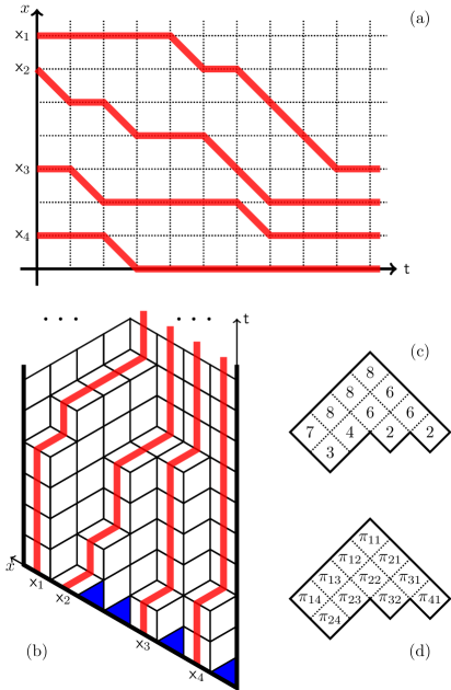
Figure 3: (a) A trajectory of the process $\Upsilon_{m}$ with $m=4$ and initial configuration $\vec{\mathsf{x}}=(7,6,3,1)$; (b) A bijective interpretation of the trajectory as a lozenge tiling (the shaded triangles correspond to $\mathbb{Z}_{\geq 0}\setminus\vec{\mathsf{x}}$ and are removed from the strip); (c) The corresponding plane partition of shape $(4,4,2,1)=(7,6,3,1)-(3,2,1,0)$; (d) Encoding the elements of the plane partition which must satisfy $\pi_{41}\geq 0$, $\pi_{32}\geq 1$, $\pi_{24}\geq 3$, and $\pi_{14}\geq 3.$

5 Plane partitions

Here we present an interpretation of trajectories of our noncolliding walks as a certain ensemble of plane partitions with an arbitrary cascade-like front wall.

5.1 Bijection to lozenge tilings and plane partitions

Let $\mathsf{t}\in\mathbb{Z}_{\geq 0}$ denote the discrete time in $\Upsilon_{m}$, and let $\vec{\mathsf{x}}(0)=\vec{\mathsf{x}}\in\mathbb{W}_{m}$ be the initial configuration of the process. Recall from Proposition 3.3 that the final configuration of the process $\Upsilon_{m}$ is $\delta_{m}=(m-1,m-2,\dots,1,0)$. Via a suitable affine transform, let us bijectively map the trajectory of $\Upsilon_{m}$ into a lozenge tiling of the vertical strip of width $\mathsf{x}_{1}+1$, see Figure 3 (a) and (b). The bottom boundary of the vertical strip is encoded by $\vec{\mathsf{x}}$ in the following way. Viewing $\vec{\mathsf{x}}$ as a particle configuration in $\mathbb{Z}_{\geq 0}$, each particle $\mathsf{x}_{i}$ corresponds to a straight piece in the boundary of slope $\big{(}{-}1/\sqrt{3}\big{)}$, and each hole corresponds to cutting a small triangle out of the strip.

Due to the absorption (Proposition 3.3), the lozenge tiling is “frozen” far at the top, with $\mathsf{x}_{1}+1-m$ tiles of one type on the left followed by $m$ tiles of the other type. Thus, the lozenge tiling contains only finitely many horizontal lozenges. Therefore, we may view the tiling as a graph of a function $\pi_{i,j}$ defined on cells of a Young diagram of size

$$\lambda=\vec{\mathsf{x}}-\delta_{m}=(\mathsf{x}_{1}-m+1,\mathsf{x}_{2}-m+2,\dots,\mathsf{x}_{m-1}-1,\mathsf{x}_{m}),$$

see Figure 3 (c) and (d). That is, in $\pi_{i,j}$ we have $1\leq i\leq m$ and $1\leq j\leq\lambda_{i}$. Since the lozenge tiling cannot have holes inside, this function must satisfy $\pi_{i,j}\geq\pi_{i+1,j}$ and $\pi_{i,j}\geq\pi_{i,j+1}$. Such functions are often called plane partitions, e.g., see [24, Chapter 7].

Moreover, due to the sloped bottom boundary of the lozenge tiling in Figure 3 (b), the plane partition must also satisfy

$$\pi_{i,\lambda_{i}}\geq\lambda_{i}-\mathsf{x}_{m}=(\mathsf{x}_{i}+i)-(\mathsf{x}_{m}+m)\qquad\text{for all $1\leq i\leq m$}.$$

This last condition means that the plane partition (or rather the corresponding lozenge tiling) has a cascade-like front wall. This front wall is encoded by the $\Upsilon_{m}$’s initial configuration $\vec{\mathsf{x}}$ which may be an arbitrary element of the space $\mathbb{W}_{m}$ (3.1).

5.2 Boltzmann factors

Fix $m\geq 1$. For a given fixed initial configuration, the space of possible trajectories of the Markov process $\Upsilon_{m}$ is countable. Here we give a different characterization of the probability measure on this space induced by the transition probabilities $\Upsilon_{m}$ (3.11). Namely, we compute the so-called Boltzmann factors, that is, the ratios of the probability weights coming from trajectories related by an elementary transformation. In this way, the probability of each given trajectory of $\Upsilon_{m}$ is proportional to the product of the Boltzmann factors associated with this trajectory. Note that such a product does not depend on the order of elementary transformations since the result is proportional to the probability (the Gibbs weight) of a trajectory which we started with.

We need some notation. Fix time $\mathsf{t}\in\mathbb{Z}_{\geq 1}$, and let $\vec{\mathsf{x}}=\vec{\mathsf{x}}(\mathsf{t}-1)$, $\vec{\mathsf{y}}=\vec{\mathsf{x}}(\mathsf{t})$, $\vec{\mathsf{z}}=\vec{\mathsf{x}}(\mathsf{t}+1)$ be three consecutive states of our Markov chain $\Upsilon_{m}$. Let us also change $\vec{\mathsf{y}}$ in an elementary way to $\vec{\mathsf{w}}$ such that for some fixed $1\leq k\leq m$:

$$\mathsf{w}_{i}=\begin{cases}\mathsf{y}_{i},&i\neq k,\\ \mathsf{y}_{k}-1,&i=k.\end{cases}$$

In the lozenge tiling interpretation of Figure 3 (b), the piece of the trajectory $\vec{\mathsf{x}}\to\vec{\mathsf{y}}\to\vec{\mathsf{z}}$ differs from $\vec{\mathsf{x}}\to\vec{\mathsf{w}}\to\vec{\mathsf{z}}$ by moving a horizontal lozenge down by $1$. Note that $\mathsf{y}_{k}=\mathsf{x}_{k}$ and $\mathsf{z}_{k}=\mathsf{w}_{k}=\mathsf{y}_{k}-1$. In the 3-dimensional interpretation of the lozenge tiling, this means removing a $1\times 1\times 1$ box from the stack of boxes. Let us also denote

$$\omega(a,b)\coloneqq\frac{\big{(}1-t^{a-b+1}q^{b-1}\big{)}\big{(}1-t^{a-b}q^{b+1}\big{)}}{\big{(}1-t^{a-b+1}q^{b}\big{)}\big{(}1-t^{a-b}q^{b}\big{)}}$$

to shorten some of the formulas below.

Proposition 5.1.

With the above notation, we have

$$\frac{\Upsilon_{m}(\vec{\mathsf{x}},\vec{\mathsf{y}})\Upsilon_{m}(\vec{\mathsf{y}},\vec{\mathsf{z}})}{\Upsilon_{m}(\vec{\mathsf{x}},\vec{\mathsf{w}})\Upsilon_{m}(\vec{\mathsf{w}},\vec{\mathsf{z}})}=t\prod_{i=1}^{k-1}\frac{\mathbf{1}_{\mathsf{z}_{i}=\mathsf{y}_{i}-1}+\omega(\mathsf{y}_{i}-\mathsf{y}_{k},k-i)\mathbf{1}_{\mathsf{z}_{i}=\mathsf{y}_{i}}}{\mathbf{1}_{\mathsf{y}_{i}=\mathsf{x}_{i}-1}+\omega(\mathsf{x}_{i}-\mathsf{x}_{k},k-i)\mathbf{1}_{\mathsf{y}_{i}=\mathsf{x}_{i}}}$$

$$\hphantom{\frac{\Upsilon_{m}(\vec{\mathsf{x}},\vec{\mathsf{y}})\Upsilon_{m}(\vec{\mathsf{y}},\vec{\mathsf{z}})}{\Upsilon_{m}(\vec{\mathsf{x}},\vec{\mathsf{w}})\Upsilon_{m}(\vec{\mathsf{w}},\vec{\mathsf{z}})}=}{}\times\prod_{j=k+1}^{m}\frac{\mathbf{1}_{\mathsf{y}_{j}=\mathsf{x}_{j}}+\omega(\mathsf{x}_{k}-\mathsf{x}_{j},j-k)\mathbf{1}_{\mathsf{y}_{j}=\mathsf{x}_{j}-1}}{\mathbf{1}_{\mathsf{z}_{j}=\mathsf{y}_{j}}+\omega(\mathsf{y}_{k}-\mathsf{y}_{j}-1,j-k)\mathbf{1}_{\mathsf{z}_{j}=\mathsf{y}_{j}-1}}.$$ (5.1)

Proof.

We use the formula

$$\Upsilon_{m}(\vec{\mathsf{x}},\vec{\mathsf{y}})=t^{-\binom{m}{2}+|\vec{\mathsf{x}}|+\sum_{i=1}^{m}(\mathsf{x}_{i}-m+i)(\mathsf{y}_{i}-\mathsf{x}_{i})}$$

$$\hphantom{\Upsilon_{m}(\vec{\mathsf{x}},\vec{\mathsf{y}})=}{}\times\frac{V_{t,q}(\vec{\mathsf{y}})}{V_{t,q}(\vec{\mathsf{x}})}\hskip 1.0pt\psi^{\prime}_{(\vec{\mathsf{x}}-\delta_{m})/(\vec{\mathsf{y}}-\delta_{m})}(t,q)\prod_{i=1}^{m}\big{(}1-q^{m-i}t^{\mathsf{x}_{i}-m+i}\mathbf{1}_{\mathsf{y}_{i}=\mathsf{x}_{i}-1}\big{)}$$

for the transition probability. Clearly, in their combination in the left-hand side of (5.1) all factors $V_{t,q}$ cancel out. Next, recall that $|\vec{\mathsf{y}}|=|\vec{\mathsf{w}}|+1$, and this gives rise to the factor $t$ in front of the right-hand side of (5.1). Next, one can readily check that all the factors coming from

$$t^{-\binom{m}{2}+\sum_{i=1}^{m}(\mathsf{x}_{i}-m+i)(\mathsf{y}_{i}-\mathsf{x}_{i})}\prod_{i=1}^{m}\big{(}1-q^{m-i}t^{\mathsf{x}_{i}-m+i}\mathbf{1}_{\mathsf{y}_{i}=\mathsf{x}_{i}-1}\big{)}$$

in the left-hand side of (5.1) cancel out, too. Finally, we are left with the ratio

$$\frac{\psi^{\prime}_{(\vec{\mathsf{x}}-\delta_{m})/(\vec{\mathsf{y}}-\delta_{m})}(t,q)\psi^{\prime}_{(\vec{\mathsf{y}}-\delta_{m})/(\vec{\mathsf{z}}-\delta_{m})}(t,q)}{\psi^{\prime}_{(\vec{\mathsf{x}}-\delta_{m})/(\vec{\mathsf{w}}-\delta_{m})}(t,q)\psi^{\prime}_{(\vec{\mathsf{w}}-\delta_{m})/(\vec{\mathsf{z}}-\delta_{m})}(t,q)}.$$

Recalling the definition of $\psi^{\prime}$ (2.8), we may rewrite this ratio as

$$\prod_{\begin{subarray}{c}1\leq i<j\leq m\\ \mathsf{y}_{i}=\mathsf{x}_{i},\,\mathsf{y}_{j}=\mathsf{x}_{j}-1\end{subarray}}\omega(\mathsf{x}_{i}-\mathsf{x}_{j},j-i)\prod_{\begin{subarray}{c}1\leq i<j\leq m\\ \mathsf{z}_{i}=\mathsf{y}_{i},\,\mathsf{z}_{j}=\mathsf{y}_{j}-1\end{subarray}}\omega(\mathsf{y}_{i}-\mathsf{y}_{j},j-i)$$

$$\qquad{}\times\prod_{\begin{subarray}{c}1\leq i<j\leq m\\ \mathsf{w}_{i}=\mathsf{x}_{i},\,\mathsf{w}_{j}=\mathsf{x}_{j}-1\end{subarray}}\frac{1}{\omega(\mathsf{x}_{i}-\mathsf{x}_{j},j-i)}\prod_{\begin{subarray}{c}1\leq i<j\leq m\\ \mathsf{z}_{i}=\mathsf{w}_{i},\,\mathsf{z}_{j}=\mathsf{w}_{j}-1\end{subarray}}\frac{1}{\omega(\mathsf{w}_{i}-\mathsf{w_{j}},j-i)}.$$

Here all terms where neither $i$ nor $j$ is equal to $k$ cancel out. When $j=k$, we may only get nontrivial contributions from the second and the third products, and when $i=k$, nontrivial contributions may only come from the first and the fourth products. In the fourth product, we use $\mathsf{w}_{k}-\mathsf{w}_{j}=\mathsf{y}_{k}-\mathsf{y}_{j}-1$. This completes the proof. ∎

In the Schur case $t=q$, we have $\omega(a,b)=1$, so the expression (5.1) reduces simply to $q$. In this way, adding a $1\times 1\times 1$ box multiplies the probability weight of a lozenge tiling by $q$, so the whole probability of a tiling is proportional to $q^{\mathsf{vol}}$, where $\mathsf{vol}$ is the volume under the corresponding 3-dimensional surface. Note that this volume is the same as the sum of the entries of the plane partition as in Figure 3 (c) and (d).

Gibbs measures on lozenge tilings of various infinite regions in which the probability weight of a tiling is proportional to $q^{\mathsf{vol}}$ have been widely studied, see, for example, [7, 21, 22]. Most well-known ensembles of such lozenge tilings are solvable by means of Schur processes, and feature an arbitrary back wall. Our ensemble of $q^{\mathsf{vol}}$ weighted lozenge tilings possesses a different kind of boundary conditions, namely, an arbitrary cascade front wall, as seen in Figure 3 (b).

Acknowledgments

I am grateful to Alexei Borodin, Grigori Olshanski, and Mikhail Tikhonov for fruitful discussions, and to the anonymous referees for helpful remarks. The work was partially supported by the NSF grant DMS-1664617, and the Simons Collaboration Grant for Mathematicians 709055. This material is based upon work supported by the National Science Foundation under Grant No. DMS-1928930 while LP participated in the program “Universality and Integrability in random matrix theory and Interacting Particle Systems” hosted by the Mathematical Sciences Research institute in Berkeley, California, during the Fall 2021 semester.

References

\LastPageEnding