Quartz: Superoptimization of Quantum Circuits (Extended Version)

Abstract.

Existing quantum compilers optimize quantum circuits by applying circuit transformations designed by experts. This approach requires significant manual effort to design and implement circuit transformations for different quantum devices, which use different gate sets, and can miss optimizations that are hard to find manually. We propose Quartz, a quantum circuit superoptimizer that automatically generates and verifies circuit transformations for arbitrary quantum gate sets. For a given gate set, Quartz generates candidate circuit transformations by systematically exploring small circuits and verifies the discovered transformations using an automated theorem prover. To optimize a quantum circuit, Quartz uses a cost-based backtracking search that applies the verified transformations to the circuit. Our evaluation on three popular gate sets shows that Quartz can effectively generate and verify transformations for different gate sets. The generated transformations cover manually designed transformations used by existing optimizers and also include new transformations. Quartz is therefore able to optimize a broad range of circuits for diverse gate sets, outperforming or matching the performance of hand-tuned circuit optimizers.

1. Introduction

Quantum computing comes in many shapes and forms. There are over a dozen proposals for realizing quantum computing in practice, and nearly all these proposals support different kinds of quantum operations, i.e., instruction set architectures (ISAs). The increasing diversity in quantum processors makes it challenging to design optimizing compilers for quantum programs, since the compilers must consider a variety of ISAs and carry optimizations specific to different ISAs.

To reduce the execution cost of a quantum circuit, the most common form of optimization is circuit transformations that substitute a subcircuit matching a specific pattern with a functionally equivalent new subcircuit with improved performance (e.g., using fewer quantum gates). Existing quantum compilers generally rely on circuit transformations manually designed by experts and applied greedily. For example, Qiskit (Aleksandrowicz et al., 2019) and t$|$ket$\rangle$ (Sivarajah et al., 2020) use greedy rule-based strategies to optimize a quantum circuit and perform circuit transformations whenever applicable. voqc (Hietala et al., 2021) formally verifies circuit transformations but still requires users manually specify them. Although rule-based transformations can reduce the cost of a quantum circuit, they have two key limitations.

First, because existing optimizers rely on domain experts to design transformations, they require significant human effort and may also miss subtle optimizations that are hard to discover manually, resulting in sub-optimal performance.

Second, circuit transformations designed for one quantum device do not directly apply to other devices with different ISAs, which is problematic in the emerging diverse quantum computing landscape. For example, IBMQX5 (Dumitrescu et al., 2018) supports the $U_{1}$, $U_{2}$, $U_{3}$ and $CNOT$ gates, while Rigetti Agave (Reagor et al., 2018) supports the $R_{x}(\pm\frac{\pi}{2})$, $R_{x}(\pi)$, $R_{z}(\lambda)$, and $CZ$ gates. As a result, circuit transformations tailored for IBMQX5 cannot optimize circuits on Rigetti Agave, and vice versa.

Recently, Quanto (Pointing et al., 2021) proposed to automatically discover transformations by computing concrete matrix representations of circuits. Its main restriction is that it does not discover symbolic transformations, which are needed to deal with common parametric quantum gates in a general way.

This paper presents Quartz, a quantum circuit superoptimizer that automatically generates and verifies symbolic circuit transformations for arbitrary gate sets, including parametric gates. Quartz provides two key advantages over existing quantum circuit optimizers. First, for a given set of gates, Quartz generates symbolic circuit transformations and formally verifies their correctness in a fully automated way, without any manual effort to design or implement transformations. Second, Quartz explores a more comprehensive set of circuit transformations by discovering all possible transformations up to a certain size, outperforming existing optimizers with manually designed transformations.

ECC sets.

We introduce equivalent circuit classes (ECCs) as a compact way to represent circuit transformations. Each ECC is a set of functionally equivalent circuits, and two circuits from an ECC form a valid transformation. We say that a transformation is subsumed by an ECC set (a set of ECCs) if the transformation can be decomposed into a sequence of transformations, each of which is a pair of circuits from the same ECC in the ECC set. We use $(n,q)$-completeness to assess the comprehensiveness of an ECC set—an ECC set is $(n,q)$-complete if it subsumes all valid transformations between circuits with at most $n$ gates and $q$ qubits.

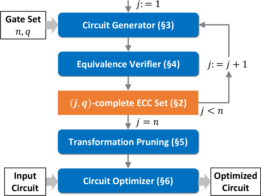
Figure 1. Quartz overview.

Overview.

Figure 1 shows an overview of Quartz, which uses an interleaving approach: it iteratively generates candidate circuits, eliminates redundancy, and verifies equivalences. In the $j$-th iteration, Quartz generates a $(j,q)$-complete ECC set based on the $(j{-}1,q)$-complete ECC set from the previous iteration. The generated ECC set may contain redundant transformations. We introduce RepGen, a representative-based circuit generation algorithm that uses a $(j{-}1,q)$-complete ECC set to generate circuits for a $(j,q)$-complete ECC set with fewer redundancies. The circuits are sent to the circuit equivalence verifier, which formally verifies equivalence between circuits and produces a $(j,q)$-complete ECC set. After generating an $(n,q)$-complete ECC set, Quartz employs several pruning techniques to further eliminate redundancies. Finally, Quartz’s circuit optimizer applies the discovered transformations to optimize an input circuit.

Circuit Generator

Given a gate set and a circuit size $n$, Quartz’s circuit generator generates candidate circuits of size at most $n$ using the RepGen algorithm, which avoids generating all possible circuits (of which there are exponentially many) while ensuring $(n,q)$-completeness. To this end, RepGen iteratively constructs ECC sets, from smaller to larger. For each ECC, RepGen selects a representative circuit and constructs larger circuits by extending these representatives.

To discover equivalences between circuits, RepGen uses random inputs to assign a fingerprint (i.e., a hash) to each circuit and checks only the circuits with the same fingerprint. We prove an upper bound on the running time of RepGen in terms of the number of representatives generated. For the gate sets considered in our evaluation, RepGen reduces the number of circuits in an ECC set by one to three orders of magnitudes while maintaining $(n,q)$-completeness.

Circuit Equivalence Verifier

Quartz’s circuit equivalence verifier checks if two potentially equivalent circuits are indeed functionally equivalent. A major challenge is dealing with gates that take one or multiple parameters (e.g., $U_{1}$, $U_{2}$, and $U_{3}$ in IBMQX5, and $R_{z}$ in Rigetti Agave). For candidate equivalent circuits, Quartz checks whether they are functionally equivalent for arbitrary combinations of parameter assignments and quantum states. To this end, Quartz computes symbolic matrix representations of the circuits. The resulting verification problem involves trigonometric functions and, in the general case, a quantifier alternation; Quartz soundly eliminates both and reduces circuit equivalence checking to SMT solving for quantifier-free formulas over the theory of nonlinear real arithmetic. The resulting SMT queries are efficiently solved by the Z3 (de Moura and Bjørner, 2008) SMT solver.

Circuit Pruning

Having generated an $(n,q)$-complete ECC set, Quartz optimizes circuits by applying the transformations specified by the ECC set. To improve the efficiency of this optimization step, described next, Quartz applies several pruning techniques to eliminate redundant transformations.

Circuit Optimizer

Quartz’s circuit optimizer uses a cost-based backtracking search algorithm adapted from TASO (Jia et al., 2019a) to apply the verified transformations. The search is guided by a cost model that compares the performance of different candidate circuits (in our experiments the cost is given by number of gates). Quartz targets the logical optimization stage in quantum circuit compilation. That is, Quartz operates before qubit mapping where logical qubits are mapped to physical qubits while respecting hardware constraints (Ding et al., 2018; Wu et al., 2021).

Evaluation

Our evaluation on three gate sets derived from existing quantum processors shows that Quartz can generate and verify circuit transformations for different gate sets in under 30 minutes (using 128 cores). For logical circuit optimization, Quartz matches and often outperforms existing optimizers. On a benchmark of 26 circuits, Quartz obtains average gate count reductions of 29%, 30%, and 49% for the Nam, IBM, and Rigetti gate sets; the corresponding reductions by existing optimizers are 27%, 23%, and 39%.

2. Symbolic Quantum Circuits

To support parametric gates, Quartz introduces symbolic quantum circuits and circuit transformations. The latter are represented compactly using equivalent circuit classes (ECCs). This section introduces these concepts.

Quantum circuits.

Quantum programs are represented as quantum circuits (Nielsen and Chuang, 2001), as shown in Figure 2(a), where each horizontal wire represents a qubit, and boxes on these wires represent quantum gates. The semantics of a quantum circuit over $q$ qubits is given by a $2^{q}\times 2^{q}$ unitary complex matrix. This matrix can be computed from matrices of individual gates in a compositional manner, using matrix multiplications (for sequential composition of subcircuits that operate on the same qubits) and tensor products (for parallel composition of subcircuits that operate on different qubits). For example, the matrix for the circuit of Figure 2(a) is $(CNOT\otimes I)\cdot(U_{2}(\frac{\pi}{2},\pi)\otimes CNOT)\cdot(U_{1}(-\pi)\otimes H\otimes H)$.

A circuit $C^{\prime}$ is a subcircuit of $C$ if, for some qubit permutation, the matrix computation for $C$ can be structured as $\mbox{\tt\char 95\relax}\cdot(M_{C^{\prime}}\otimes I\otimes\cdots\otimes I)\cdot\mbox{\tt\char 95\relax}$, where $M_{C^{\prime}}$ is the matrix for $C^{\prime}$. For example, the green box in Figure 2(a) highlights a subcircuit, while the red dashed area is not a subcircuit. The subcircuit notion is invariant under qubit permutation; e.g., the $X$ and $U_{1}$ gates in Figure 2(a) also form a subcircuit. A circuit’s matrix is invariant under replacing one subcircuit with another that has the same matrix (but possibly different gates), which underpins peephole optimization for quantum circuits.

Many gates supported by modern quantum devices take real-valued parameters. For example, the IBM quantum device supports the $U_{1}$ gate which takes one parameter and rotates a qubit about the $x$-axis (on the Bloch sphere), and the $U_{2}$ gate which takes two parameters for rotating about the $x$- and $z$-axes. The matrix representations of $U_{1}$ and $U_{2}$ are:

(1) $$U_{1}(\theta)=\begin{pmatrix}1&0\\ 0&e^{i\theta}\end{pmatrix}\quad U_{2}(\phi,\lambda)=\frac{1}{\sqrt{2}}\begin{pmatrix}1&-e^{i\lambda}\\ e^{i\phi}&e^{i(\phi+\lambda)}\end{pmatrix}$$

(a) Quantum circuit.

(b) Symbolic Quantum circuit.

(c) Transformation fusing two $R_{z}$ gates across $CZ$ and $X$ gates.

Figure 2. Quantum circuits and transformations. The green highlighted box in (a) is a subcircuit, while the red dashed area is not; the $U_{1}(-\pi)$ and $X$ gates also form a subcircuit.

Symbolic circuits.

To support superoptimization of circuits with parametric gates, Quartz discovers transformations between symbolic quantum circuits, as shown in Figure 2(b), which include (symbolic) parameters ($\theta$, $\phi$, $\lambda$, $\delta$, etc.) and arithmetic operations on these parameters, and are formalized below. Using such circuits, Quartz can represent transformations such as the one illustrated in Figure 2(c).

The semantics of a symbolic quantum circuit, denoted $\llbracket{\cdot}\rrbracket$, has type $\llbracket{C}\rrbracket\colon\mathbb{R}^{m}\rightarrow\mathbb{C}^{2^{q}\times 2^{q}}$ where $C$ is a circuit over $m$ (symbolic) parameters and $q$ qubits. For a vector of parameter values $\vec{p}\in\mathbb{R}^{m}$, $\llbracket{C}\rrbracket(\vec{p})$ is a $2^{q}\times 2^{q}$ unitary complex matrix representing a (concrete) quantum circuit over $q$ qubits. For example, eq. 1 can be seen as defining the semantics of $U_{1}$ and $U_{2}$ as single-gate symbolic quantum circuits. The semantics of a multi-gate symbolic circuit (e.g., Figure 2(b)) is derived from that of single-gate circuits using matrix multiplications and tensor products exactly as for concrete circuits. Henceforth, we use circuits to mean symbolic quantum circuits.

Circuit equivalence and transformations.

In quantum computing, the states $\ket{\psi}$ and $e^{i\beta}\ket{\psi}$ ($\beta\in\mathbb{R}$) are equivalent up to a global phase, and from an observational point of view they are identical (Nielsen and Chuang, 2001). This leads to the following circuit-equivalence definition that underlies Quartz’s optimization.

Definition 0 (Circuit Equivalence).

Two symbolic quantum circuits $C_{1}$ and $C_{2}$ are equivalent if:

(2) $$\forall\vec{p}\in\mathbb{R}^{m}.\;\exists\beta\in\mathbb{R}.\;\llbracket{C_{1}}\rrbracket(\vec{p})=e^{i\beta}\llbracket{C_{2}}\rrbracket(\vec{p}).$$

That is, two circuits are equivalent if for every valuation of the parameters they differ only by a phase factor. The phase factor may in some cases be constant, but generally it may be different for different parameter values. For example, the equivalence between $U_{1}$ and $R_{z}$ gates ($U_{1}(\theta)=e^{i\theta/2}R_{z}(\theta)$) requires a parameter-dependent phase factor. Crucially for peephole optimization, circuit equivalence is invariant under replacing a subcircuit with an equivalent subcircuit.

A circuit transformation $(C_{T},C_{R})$ is a pair of distinct equivalent circuits, where $C_{T}$ is a target circuit to be matched with a subcircuit of the circuit being optimized, and $C_{R}$ is a rewrite circuit that can replace the target circuit while maintaining equivalence of the optimized circuit and the input circuit. Figure 2(c) illustrates a circuit transformation.

(a) Common optimization removing four Hadamard gates.

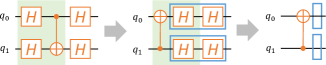
(b) Above optimization as a circuit rewriting using transformations.

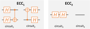
(c) An ECC set that includes the transformations used above.

Figure 3. Illustrating optimization via transformations.

Equivalent Circuit Classes

Quartz uses equivalent circuit classes (ECCs), to represent many circuit transformations compactly. An ECC is a set of equivalent circuits. A transformation is included in an ECC if both its target and rewrite circuits are in the ECC. ECCs provide a compact representation of circuit transformations: an ECC with $x$ circuits includes $x(x-1)$ transformations.

A circuit rewriting is a sequence of applications of circuit transformations, which Quartz uses for optimization as illustrated in Figure 3. Figure 3(a) shows a common optimization that removes four Hadamard gates (i.e., $H$) by flipping a $CNOT$ gate. Figure 3(b) shows how to perform this optimization as a circuit rewriting consisting of three (more basic) circuit transformations, which are instances of the two transformations specified by the ECC set in Figure 3(c).

Completeness for ECC sets.

For any number of gates $n$, qubits $q$, and parameters $m$, we assume a finite set $\mathcal{C}^{(n,q,m)}$ of circuits that can be constructed with at most $n$ gates over $q$ qubits and $m$ parameters. The collection $\{\mathcal{C}^{(n,q,m)}\}_{n,q,m\in\mathbb{N}}$ is determined by the gate set $\mathcal{G}$ (finite set of possibly parametric gates) as well as a specification $\Sigma$ of how parameter expressions may be constructed; e.g., a finite set of arithmetic operations and some bounds on the depth of expressions or the number of times each parameter can be used, ensuring finiteness of every $\mathcal{C}^{(n,q,m)}$. Henceforth, we fix the gate set $\mathcal{G}$, the parameter-expression specification $\Sigma$, and the number of parameters $m$; and elide $m$ by writing $\mathcal{C}^{(n,q)}$.

A transformation $(C_{T},C_{R})$ is subsumed by an ECC set if there is a circuit rewriting from $C_{T}$ to $C_{R}$ that only uses transformations included in the ECC set.

Definition 0 ($(n,q)$-Completeness).

Given $\mathcal{G}$, $\Sigma$, and $m$ as above, an ECC set is $(n,q)$-complete (for $\mathcal{G}$, $\Sigma$, and $m$) if it subsumes all circuit transformations over $\mathcal{C}^{(n,q)}$.

An $(n,q)$-complete ECC set can be used to rewrite any two equivalent circuits with at most $n$ gates over $q$ qubits to each other. Any ECC set is by default $(0,q)$-complete because any transformation involves at least one gate in the target or rewrite circuits. An ECC set is $(1,q)$-complete if it subsumes all possible transformations between single gates. Sections 3, 4 and 5 describe our approach for constructing a verified $(n,q)$-complete ECC set.

3. Circuit Generator

Quartz builds an $(n,q)$-complete ECC set using the RepGen algorithm, developed in this section, which interleaves circuit generation and equivalence verification (see Figure 1).

3.1. The RepGen Algorithm

A straightforward way to generate an $(n,q)$-complete ECC set is to examine all circuits in $\mathcal{C}^{(n,q)}$, but there are exponentially many such circuits. To tackle this challenge, RepGen uses representative-based circuit generation, which significantly reduces the number of circuits considered. The key idea is to extend a $(j,q)$-complete ECC set to a $(j+1,q)$-complete one by selecting a representative circuit for each ECC and using these representatives to build larger circuits.

Algorithm 1 RepGen.

1:Input: Number of gates $n$ and qubits $q$.

2:Output: $(n,q)$-complete ECC set.

3:$\mathcal{D}=\emptyset$ // Hash table of circuit sets indexed by fingerprint

4:$\mathcal{D}[\textsc{FingerPrint}(())]=\{()\}$ // Initialize with empty circuit

5:$\mathcal{R}_{0}=\{()\}$ // Representatives with 0 gates

6:$\mathcal{S}_{0}=\emptyset$ // $(0,q)$-complete ECC set

7:for $j=1$ to $n$ do

8:    // Step 1: construct circuits (sequences) with $j$ gates

9:    for each circuit $L\in\mathcal{R}_{j-1}$ such that $|L|=j-1$ do

10:         for each gate $g\in\mathcal{G}$ do

11:             for each $\iota$ such that $L^{\prime}=L.(g\ \iota)$ satisfies $\Sigma$ do

12:                 if $\textsc{DropFirst}(L^{\prime})\in\mathcal{R}_{j-1}$ then

13:                     add $L^{\prime}$ to $\mathcal{D}[\textsc{FingerPrint}(L^{\prime})]$                                            

14:    // Step 2: examine circuits with equal fingerprints

15:    $\mathcal{S}_{j}=\bigcup\{\textsc{Eccify}(\gamma):\gamma=\mathcal{D}[f]\text{ for some }f\}$

16:    $\mathcal{R}_{j}=\{\mbox{\rm\em min}(\mathcal{E}):\mathcal{E}\in\mathcal{S}_{j}\}$ // Under $\prec$ (Definition 1)

17:return $\{\mathcal{E}\in\mathcal{S}_{n}:|\mathcal{E}|\geq 2\}$ // Ignore singleton ECCs

18:

19:// Partition circuits into verified ECCs

20:function Eccify($\gamma$)

21:    $\widehat{\mathcal{S}}=\emptyset$ // Set of ECCs for circuits in $\gamma$

22:    for each circuit $C\in\gamma$ do

23:         if $C$ is equivalent to a circuit in ECC $\mathcal{E}\in\widehat{\mathcal{S}}$ then

24:             $\widehat{\mathcal{S}}=\widehat{\mathcal{S}}\setminus\{\mathcal{E}\}\cup\{\mathcal{E}\cup\{C\}\}$ // Add $C$ to $\mathcal{E}$

25:         else

26:             $\widehat{\mathcal{S}}=\widehat{\mathcal{S}}\cup\{\{C\}\}$ // Create a new ECC for $C$              

27:    return $\widehat{\mathcal{S}}$

Sequence representation for circuits.

RepGen represents a circuit as a sequence of instructions that reflects a topological ordering of its gates (i.e., respecting dependencies). E.g., a possible sequence for the circuit in Figure 2(b) is: U1 $\theta$ 0; U2 $2\phi$ $\lambda{+}\delta$ 0; H 1; X 2; CNOT 1 2; CNOT 0 1.We write $()$ for the empty sequence and $L.(g\ \iota)$ for appending gate $g\in\mathcal{G}$ with arguments $\iota$ (parameter expressions and qubit indices) to sequence $L$; e.g., for the second instruction above $g=\texttt{U2}$ and $\iota=(2\phi,\lambda{+}\delta,0)$. Different sequences may represent the same circuit; e.g. the U2 and X instructions above can be swapped. RepGen eliminates some of this representation redundancy by the same mechanism it uses for avoiding redundancy due to circuit equivalence.

We use $|L|$, $\textsc{DropFirst}(L)$, and $\textsc{DropLast}(L)$ to denote the number of gates in a circuit $L$, its suffix with $|L|-1$ gates, and its prefix with $|L|-1$ gates. Note that each of the latter two represents a subcircuit.

We fix an arbitrary total order over single-gate circuits (i.e., $\mathcal{C}^{(1,q)}$), and lift it to a total order of circuits (i.e., sequences).

Definition 0 (Circuit Precedence).

We say $L_{1}$ precedes $L_{2}$, written $L_{1}\prec L_{2}$, if $|L_{1}|<|L_{2}|$, or if $|L_{1}|=|L_{2}|$ and $L_{1}$ is lexicographically smaller than $L_{2}$.

Algorithm 1 lists the RepGen algorithm, which proceeds in rounds and maintains a database $\mathcal{D}$ of circuits grouped by fingerprints (defined below), a $(j,q)$-complete ECC set $\mathcal{S}_{j}$, and a representative set (set of representatives) $\mathcal{R}_{j}$ for ECCs in $\mathcal{S}_{j}$. The $j$-th round produces a $(j,q)$-complete ECC set from the $(j-1,q)$-complete ECC set generated in the previous round. Each round proceeds in two steps.

Step 1: Constructing circuits.

Before the first round, the initial ECC set is $\mathcal{S}_{0}=\emptyset$ and the representative set is $\mathcal{R}_{0}=\{()\}$, i.e., a singleton set consisting of the empty circuit (over $q$ qubits). In the $j$-th round, RepGen uses the $(j{-}1,q)$-complete ECC set $\mathcal{S}_{j-1}$ and its representative set $\mathcal{R}_{j-1}$ computed previously, and constructs possible size-$j$ circuits by appending a single gate to each circuit in $\mathcal{R}_{j-1}$ with size $j-1$. RepGen enumerates all possible gates $g$ and arguments $\iota$ according to $\mathcal{G}$ and $\Sigma$. For each generated circuit $L^{\prime}$, RepGen checks if $\textsc{DropFirst}(L^{\prime})$ is a representative from the previous round. If so, RepGen concludes that $L^{\prime}$ extends existing representatives and must be considered in generating $\mathcal{S}_{j}$. Otherwise, circuit $L^{\prime}$ is considered redundant and ignored. We prove the correctness of RepGen in Theorem 3.

To identify potentially equivalent circuits, RepGen computes circuit fingerprints, and uses them as keys for storing circuits in the hash table $\mathcal{D}$. The fingerprint is computed using fixed, randomly selected parameter values and quantum states. Recall that for a circuit $C$ over $q$ qubits and $m$ parameters, and parameter values $\vec{p}\in\mathbb{R}^{m}$, $\llbracket{C}\rrbracket(\vec{p})$ is a (concrete) $2^{q}\times 2^{q}$ complex matrix. The fingerprint of a circuit $C$ is

(3) $$\textsc{FingerPrint}(C)=\left|\bra{\psi_{0}}\llbracket{C}\rrbracket(\vec{p_{0}})\ket{\psi_{1}}\right|,$$

where the parameter values $\vec{p_{0}}$ and quantum states $\ket{\psi_{0}}$ and $\ket{\psi_{1}}$ are fixed and randomly selected, and $|\cdot|$ denotes modulus of a complex number. With infinite precision, eqs. 2 and 3 ensure that equivalent circuits have identical fingerprints. This section presents and analyzes RepGen assuming infinite precision, while Section 7.1 presents an adaptation for finite-precision floating-point arithmetic.

Step 2: Examining circuits with equal fingerprints.

In Step 1, RepGen generates circuits and stores them in the hash table $\mathcal{D}$ grouped by their fingerprints. In Step 2, RepGen partitions each set $\gamma=\mathcal{D}[f]$ of potentially equivalent circuits into a verified ECC set using the function Eccify. Eccify considers each circuit in $\gamma$ and checks if it is equivalent to some existing ECC in $\gamma$ by querying the verifier (Section 4); the circuit is then either added to the matching ECC, or becomes a new singleton ECC. RepGen then combines the ECC sets for each $\gamma$ to get the ECC set $\mathcal{S}_{j}$.

Having constructed an ECC set $\mathcal{S}_{j}$, RepGen computes $\mathcal{S}_{j}$’s representative set $\mathcal{R}_{j}$, which is the set of representatives of the ECCs in $\mathcal{S}_{j}$ (Algorithm 1 line 16). The representative of an ECC is its $\prec$-minimum circuit (Definition 1). During the operation of RepGen, singleton ECCs are important: their representatives must be considered when generating circuits in the next round, and they may grow to non-singleton ECCs as more circuits are generated. However, singleton ECCs in $\mathcal{S}_{n}$ ultimately yield no transformations, so we remove them from the result of the RepGen algorithm (line 17).

3.2. Correctness of RepGen

When constructing circuits of size $j$ (in round $j$), RepGen only considers circuits $L^{\prime}$ that extend previously constructed representatives, i.e., $\textsc{DropLast}(L^{\prime})\in\mathcal{R}_{j-1}$, and only when the extension leads to $\textsc{DropFirst}(L^{\prime})\in\mathcal{R}_{j-1}$. In this section we prove that in spite of that, RepGen always generates an $(n,q)$-complete ECC set. Below we use $\mathcal{D}_{j}$ to denote the value of $\mathcal{D}$ after Step 1 in RepGen’s $j$-th round (i.e., at Algorithm 1 line 15) and $\mathcal{D}_{0}$ for the initial value of $\mathcal{D}$ (line 4).

Lemma 2.

Algorithm 1 maintains the following invariants (for any $1\leq j\leq n$, and writing $\sqsubseteq$ for Hoare ordering, i.e., $\mathcal{X\sqsubseteq Y}\equiv\forall X\in\mathcal{X}.\,\exists Y\in\mathcal{Y}.\,X\subseteq Y$):

1. $\mathcal{D}_{j-1}\sqsubseteq\mathcal{D}_{j}$, $\mathcal{S}_{j-1}\sqsubseteq\mathcal{S}_{j}$, and $\mathcal{R}_{j-1}\subseteq\mathcal{R}_{j}$;

2. for any $L\in\mathcal{C}^{(n,q)}$, $L\in\bigcup\mathcal{D}_{j}$ iff $|L|\leq j$ and either $L=()$ or $\textsc{DropFirst}(L),\textsc{DropLast}(L)\in\mathcal{R}_{j-1}$; and

3. for any $L\in\mathcal{C}^{(n,q)}$, $L\in\mathcal{R}_{j}$ iff $|L|\leq j$ and $L$ does not have a $\prec$-smaller equivalent circuit in $\mathcal{C}^{(n,q)}$.

Proof.

For item 1, $\mathcal{D}_{j-1}\sqsubseteq\mathcal{D}_{j}$ and $\mathcal{S}_{j-1}\sqsubseteq\mathcal{S}_{j}$ follow from the monotonic updating of $\mathcal{D}$ (i.e., circuits are only added), and from monotonicity (w.r.t. Hoare ordering) of Eccify. To see that $\mathcal{R}_{j-1}\subseteq\mathcal{R}_{j}$, observe that in the $j$-th round, all circuits constructed are of size $j$, so any circuit added to an existing ECC has more gates than its representative in $\mathcal{R}_{j-1}$, which will therefore remain its representative in $\mathcal{R}_{j}$ (recall that if $|L|<|L^{\prime}|$ then $L\prec L^{\prime}$).

We prove item 2 by induction on $j$. Both the base case ($j=1$) and the induction step follow from Algorithm 1 lines 9–13, combined with item 1 and either the definition of $\mathcal{D}_{0}$ or the induction hypothesis.

We prove item 3 by induction on $j$. Slightly generalizing from the statement above, we take the base case to be $j=0$, which follows from line 5. In the induction step, for sufficiency, consider a circuit $L$, $1\leq|L|\leq j$, with no $\prec$-smaller equivalent circuit. (The $|L|=0$ case follows from line 5 and item 1.) Both $\textsc{DropFirst}(L)$ and $\textsc{DropLast}(L)$ are of size $\leq j-1$ with no $\prec$-smaller equivalent circuits (if either had a $\prec$-smaller equivalent circuit, we could use it to construct a $\prec$-smaller equivalent circuit for $L$). By the induction hypothesis, $\textsc{DropFirst}(L),\textsc{DropLast}(L)\in\mathcal{R}_{j-1}$, so by item 2, $L\in\bigcup\mathcal{D}_{j}$. By lines 15–16, $\mathcal{R}_{j}$ includes the $\prec$-minimal element of each class of equivalent circuits in $\bigcup\mathcal{D}$, so it must include $L$. Necessity follows from sufficiency, combined with the fact that two circuits in $\mathcal{R}_{j}$ cannot be equivalent and that $\mathcal{R}_{j}$ does not contain circuits of size greater than $j$. ∎

Theorem 3 (RepGen).

In Algorithm 1, every $\mathcal{S}_{j}$ ($0\leq j\leq n$) is a $(j,q)$-complete ECC set, and the algorithm returns an $(n,q)$-complete ECC set.

Proof.

We proceed using proof by contradiction. Let $j$ be the smallest such that $\mathcal{S}_{j}$ is not $(j,q)$-complete. We must have $j>0$, with $\mathcal{S}_{j-1}$ $(j{-}1,q)$-complete, and by Lemma 2 item 1 $\mathcal{S}_{j}$ is also $(j{-}1,q)$-complete. (As $\mathcal{S}_{j-1}\sqsubseteq\mathcal{S}_{j}$, $\mathcal{S}_{j}$ only includes more transformations.) Let $(L,L^{\prime})$ be the minimal (under the pairwise lexicographic lifting of $\prec$) pair of equivalent circuits of size $\leq j$ that cannot be rewritten to each other using transformations included in $\mathcal{S}_{j}$. We must have $|L^{\prime}|=j$, since otherwise $|L|,|L^{\prime}|\leq j-1$, but $\mathcal{S}_{j}$ is $(j{-}1,q)$-complete.

If $\textsc{DropFirst}(L^{\prime})$ has a $\prec$-smaller equivalent circuit, then $\mathcal{S}_{j}$ can rewrite $L^{\prime}$ to a $\prec$-smaller equivalent circuit, which it must also not be able to rewrite to $L$, contradicting the minimality of $L^{\prime}$. Therefore, $\textsc{DropFirst}(L^{\prime})$ does not have a $\prec$-smaller equivalent circuit; The same argument works for $\textsc{DropLast}(L^{\prime})$. Therefore, by using Lemma 2 item 3 we get $\textsc{DropFirst}(L^{\prime}),\textsc{DropLast}(L^{\prime})\in\mathcal{R}_{j-1}$, and by Lemma 2 item 2, $L^{\prime}\in\mathcal{D}_{j}$. But if $L^{\prime}\in\mathcal{D}_{j}$ then either $\mathcal{S}_{j}$ includes a transformation that rewrites $L^{\prime}$ to a smaller equivalent circuits, that it cannot rewrite to $L$, contradicting the minimality of $L^{\prime}$; or $L^{\prime}$ does not have a $\prec$-smaller equivalent circuit, contradicting the definition of the pair $(L,L^{\prime})$. ∎

3.3. Complexity of RepGen

We analyze the time complexity of RepGen (its space complexity is the same). First, observe that the number of single-gate circuits $|\mathcal{C}^{(1,q)}|-1$, which is determined by the gate set $\mathcal{G}$, parameter-expression specification $\Sigma$, number of qubits $q$, and parameters $m$, provides an upper bound for the number of single-gate extensions of any existing circuit. (The $-1$ is due to $()\in\mathcal{C}^{(1,q)}.)$ This characteristic of $\mathcal{G}$, $\Sigma$, $q$, and $m$, denoted $\mathrm{ch}(\mathcal{G},\Sigma,q,m)=|\mathcal{C}^{(1,q)}|-1$, bounds the number of iterations of the loops in Algorithm 1 lines 10 and 11 in each round. (The bound may not be tight as $\Sigma$ may impose more restrictions, e.g., single use of parameters.)

While $\sum_{j=0}^{n}\mathrm{ch}(\mathcal{G},\Sigma,q,m)^{j}$ provides a trivial upper bound on the complexity of RepGen, the following theorem shows that RepGen’s running time can be bounded using the number of resulting representatives $|\mathcal{R}_{n}|$. In practice, this number is significantly smaller than $\mathrm{ch}(\mathcal{G},\Sigma,q,m)^{n}$ (see Table 5).

Theorem 4 (Complexity of RepGen).

The time complexity of Algorithm 1, excluding the verification part (line 15), is

$$O\big{(}|\mathcal{R}_{n}|\cdot\mathrm{ch}(\mathcal{G},\Sigma,q,m)\cdot n\big{)}.$$

Proof.

The $j$-th round of Algorithm 1 considers circuits from $\mathcal{R}_{j-1}$ with size $j-1$, and for each one it considers at most $\mathrm{ch}(\mathcal{G},\Sigma,q,m)$ possible extensions. It takes $O(n)$ to construct a new circuit and add it to $\mathcal{D}$. (We assume $O(1)$ complexity for hash table insert and lookup, i.e., we use average and amortized complexity.) Summing over all rounds of Algorithm 1, and recalling that $\mathcal{R}_{j}\subseteq\mathcal{R}_{n}$ (Lemma 2 item 1):

$$\sum_{j=1}^{n}|\{L\in\mathcal{R}_{j-1}:|L|=j-1\}|\cdot\mathrm{ch}(\mathcal{G},\Sigma,q,m)\cdot n$$

$$\leq |\mathcal{R}_{n}|\cdot\mathrm{ch}(\mathcal{G},\Sigma,q,m)\cdot n.$$

∎

Note that if $\mathcal{G}$, $\Sigma$, $q$, and $m$ are considered as constant then the time complexity of Algorithm 1 is $O(|\mathcal{R}_{n}|\cdot n)$.

Table 5 lists some empirical $\mathrm{ch}(\mathcal{G},\Sigma,q,m)$ and $|\mathcal{R}_{n}|$ values.

4. Circuit Equivalence Verifier

Given two circuits $C_{1}$ and $C_{2}$ over $q$ qubits and $m$ parameters, the verifier checks if they are equivalent (i.e., up to a global phase). Recalling eq. 2, that means checking if $\forall\vec{p}\in\mathbb{R}^{m}.\;\exists\beta\in\mathbb{R}.\;\llbracket{C_{1}}\rrbracket(\vec{p})=e^{i\beta}\llbracket{C_{2}}\rrbracket(\vec{p})$. Note that the equality here is between two $2^{q}\times 2^{q}$ complex matrices.

There are two challenges in automatically checking eq. 2. One is the quantifier alternation, which may be needed to account for global phase; the other is the use of trigonometric function, which is common in quantum gates’ matrix representations. For example, the $U_{3}$ gate supported by the IBM quantum processors has the following matrix representation:

(4) $$\llbracket{U_{3}}\rrbracket(\theta,\phi,\lambda)=\begin{pmatrix}\cos(\frac{\theta}{2})&-e^{i\lambda}\sin(\frac{\theta}{2})\\ e^{i\phi}\sin(\frac{\theta}{2})&e^{i(\phi+\lambda)}\cos(\frac{\theta}{2})\end{pmatrix}.$$

While some SMT solvers support quantifiers and trigonometric functions (Barrett et al., 2011; Cimatti et al., 2017), our preliminary attempts showed they cannot directly prove eq. 2 for the circuit transformations generated by Quartz. Our verification approach is therefore to reduce eq. 2 to a quantifier-free formula over nonlinear real arithmetic by eliminating both the quantification over $\beta$ and the trigonometric functions. The resulting verification conditions are then checked using the Z3 (de Moura and Bjørner, 2008) SMT solver. This approach can efficiently verify all circuit transformations generated in our experiments (Section 7.4).

Phase factors

To eliminate the existential quantification over the phase $\beta$, we search over a finite space of linear combinations of the parameters $\vec{p}$ for a value that can be used for $\beta$. We consider $\beta(\vec{p})=\vec{a}\cdot\vec{p}+b$, where $\vec{a}\in A$ and $b\in B$ for some finite sets $A\subseteq\mathbb{R}^{m}$ and $B\subseteq\mathbb{R}$. (Our experimentation with various combinations of quantum gates suggested that $\vec{a}\neq\vec{0}$ is sometimes needed, so we develop the mechanism with this generality; however, in the experiments reported in Section 7, constant phase factors, i.e. $\vec{a}=\vec{0}$, turned out to be sufficient for the three gate sets and the parameter specifications used.) Given circuits $C_{1}$ and $C_{2}$, we find candidates for the coefficients $\vec{a}$ and $b$ using an approach similar to the one we use for generating candidate transformations. We select random parameter values $\vec{p_{0}}$ and quantum states $\ket{\psi_{0}}$ and $\ket{\psi_{1}}$ and find all combinations of $\vec{a}$ and $b$ as above that satisfy the following equation up to a small floating-point error (note that unlike eq. 3, $|\cdot|$ is not used):

(5) $$\bra{\psi_{0}}\llbracket{C_{1}}\rrbracket(\vec{p_{0}})\ket{\psi_{1}}=e^{i(\vec{a}\cdot\vec{p}+b)}\cdot\bra{\psi_{0}}\llbracket{C_{2}}\rrbracket(\vec{p_{0}})\ket{\psi_{1}},$$

For every such candidate coefficients $\vec{a}$ and $b$, we then attempt to verify following equation,

(6) $$\forall\vec{p}\in\mathbb{R}^{m}.\;\llbracket{C_{1}}\rrbracket(\vec{p})=e^{i(\vec{a}\cdot\vec{p}+b)}\llbracket{C_{2}}\rrbracket(\vec{p}),$$

which unlike eq. 2, does not existentially quantify over $\beta$. If eq. 6 holds for some candidate coefficients, then $C_{1}$ and $C_{2}$ are verified to be equivalent. Otherwise, we consider the transformation given by $C_{1}$ and $C_{2}$ to fail verification, but that case did not occur in our experiments.

Trigonometric functions

Matrices of parametric quantum gates we encountered only use their parameters inside arguments to $\sin$ or $\cos$ (after applying Euler’s formula). Under this assumption, we reduce eq. 6 to nonlinear real arithmetic in three steps. First, we eliminate expressions such as $\frac{\theta}{2}$ that occur in some quantum gates (e.g., eq. 4) by introducing a fresh variable $\theta^{\prime}=\frac{\theta}{2}$ and substituting $\theta^{\prime}+\theta^{\prime}$ for $\theta$. After this step, all arguments to $\sin$ and $\cos$ are linear combinations of variables and constants (e.g., from phase factors) with integer coefficients. Second, we exhaustively apply Euler’s formula $e^{i\phi}=\cos\phi+i\sin\phi$, and trigonometric identities for parity and sum of angles: $\sin(-x)=-\sin(x)$, $\cos(-x)=\cos(x)$, $\sin(x+y)=\sin(x)\cos(y)+\cos(x)\sin(y)$, and $\cos(x+y)=\cos(x)\cos(y)-\sin(x)\sin(y)$. After these steps, $\sin$ and $\cos$ are only applied to atomic terms (variables and constants). For each constant $c$, we require precise symbolic expressions for $\sin(c)$ and $\cos(c)$ (e.g., $\sin(\frac{\pi}{4})=\frac{\sqrt{2}}{2}$), and eliminate $\sin$ and $\cos$ over constants using these expressions. Third, for every variable $t$ such that $\sin(t)$ or $\cos(t)$ is used we substitute $s_{t}$ for $\sin(t)$ and $c_{t}$ for $\cos(t)$, where $s_{t}$ and $c_{t}$ are fresh variables with a constraint $s_{t}^{2}+c_{t}^{2}=1$, which fully eliminates trigonometric functions.

Ultimately, Z3 can check the transformed version of eq. 6 using the theory of quantifier-free nonlinear real arithmetic.

During the development of Quartz we occasionally encountered verification failures, but these were due to implementation bugs, and the counterexamples obtained from Z3 were useful in the debugging process. Thus, verification is useful not only to ensure the ultimate correctness of the generated transformations, but also in the development process.

5. Pruning Redundant Transformations

(a) A circuit transformation.

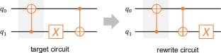
(b) Redundant circuit transformation (common subcircuit).

Figure 4. Illustrating a redundant circuit transformation.

Quartz applies two pruning steps after RepGen generates an $(n,q)$-complete ECC set to further eliminate redundancy. These steps maintain $(n,q)$-completeness while reducing the number of transformations the optimizer needs to consider.

5.1. ECC Simplification

All ECCs generated by RepGen have circuits with exactly $q$ qubits. For each ECC, a qubit (or a parameter) is unused if all circuits in the ECC do not operate on the qubit (or the parameter). An ECC simplification pass removes all unused qubits and parameters from each ECC. After this pass, some ECCs may become identical, among which only one is kept.

Because there is no specific order on parameters in a circuit, Quartz also finds identical ECCs under a permutation of the parameters and maintains only one of them.

5.2. Common Subcircuit Pruning

Quartz eliminates transformations whose target and rewrite circuits include a common subcircuit at the beginning or the end. Figure 4 illustrates this common subcircuit pruning; the common subcircuit is highlighted in grey. Theorem 2 explains why such transformations are always redundant.

Definition 0.

A subset of gates $C^{\prime}$ in a circuit $C$ is a subcircuit at the beginning of $C$ if all gates in $C^{\prime}$ are topologically before all gates in $C\setminus C^{\prime}$. Similarly, a subset of gates $C^{\prime}$ in a circuit $C$ is a subcircuit at the end of $C$ if all gates in $C^{\prime}$ are topologically after all gates in $C\setminus C^{\prime}$.

Theorem 2.

For any two quantum circuits $C_{1}$ and $C_{2}$ with a common subcircuit at the beginning or the end, if $C_{1}$ and $C_{2}$ are equivalent, then eliminating the common subcircuit from $C_{1}$ and $C_{2}$ generates two equivalent circuits.

Proof.

Recall that $\llbracket{C}\rrbracket(\vec{p})$ (for all $\vec{p}$—we elide $\vec{p}$ in this proof) denotes the matrix representation of circuit $C$. Let $\llbracket{C}\rrbracket^{\dagger}$ be the conjugate transpose of $\llbracket{C}\rrbracket$, and recall that as $\llbracket{C}\rrbracket$ is unitary, we have $\llbracket{C}\rrbracket^{\dagger}\llbracket{C}\rrbracket=\llbracket{C}\rrbracket\llbracket{C}\rrbracket^{\dagger}=I$. Let $C_{s}$ denote the common subcircuit shared by $C_{1}$ and $C_{2}$. Let $C_{1}^{\prime}$ and $C_{2}^{\prime}$ represent the new circuits obtained by removing $C_{s}$ from $C_{1}$ and $C_{2}$. When $C_{s}$ is a common subcircuit at the beginning of $C_{1}$ and $C_{2}$, the matrix representations for the new circuits are $\llbracket{C_{i}^{\prime}}\rrbracket=\llbracket{C_{s}}\rrbracket^{\dagger}\llbracket{C_{i}}\rrbracket$, where $i=1,2$. Equivalence between $C_{1}$ and $C_{2}$ implies the existence of $\beta$ such that $\llbracket{C_{1}}\rrbracket=e^{i\beta}\llbracket{C_{2}}\rrbracket$, therefore $\llbracket{C_{1}^{\prime}}\rrbracket=e^{i\beta}\llbracket{C_{2}^{\prime}}\rrbracket$. The case where $C_{s}$ is a common subcircuit at the end is similar. ∎

Theorem 2 shows that every transformation pruned in common subcircuit pruning must be subsumed by other transformations (assuming initial $(n,q)$-completeness).

Observe that if two circuits have a common subcircuit at the beginning (resp. the end), then they must have a common gate at the beginning (resp. the end). Therefore, to implement common subcircuit pruning, Quartz only checks for a single common gate at the beginning or the end.

6. Circuit Optimizer

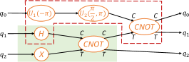
Figure 5. Graph representation for Figure 2(a)’s circuit. The green box (subcircuit, also convex subgraph) and red dashed area (not a subcircuit, also non-convex subgraph) match those of Figure 2(a).

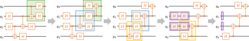
Figure 6. A transformation sequence applied by Quartz that reduces the total gate count in the gf2^4_mult circuit by swapping the control and target qubits of three $CNOT$ gates. Note that the first three transformations do not reduce gate count.

Quartz’s circuit optimizer applies the verified transformations generated by the generator to find an optimized equivalent circuit for a given input circuit (see Figure 1).

A key step is computing $\textsc{Apply}(C,T)$, the set of circuits that can be obtained by applying transformation $T=(C_{T},C_{R})$ to circuit $C$. This involves finding all possible ways to match $C_{T}$ with a subcircuit of $C$. Quartz’s optimizer uses a graph representation for circuits, explained below, to implement this operation. In the graph representation, subcircuits correspond to convex subgraphs, and Quartz adapts the graph-matching procedure from TASO (Jia et al., 2019a) to find all matches between $C_{T}$ and a convex subgraph of $C$.

In the graph representation, a circuit $C$ over $q$ qubits is represented as a directed graph $G$, where each gate over $d$ qubits is a vertex with in- and out-degree $d$. Edges are labeled to distinguish between qubits in multi-qubit gates (e.g., the control and target qubits of a $CNOT$ gate). $G$ also includes $q$ sources and sinks, one for each qubit. Figure 5 illustrates the graph representation of Figure 2(a)’s circuit. As the figure also illustrates, subcircuits correspond to convex subgraphs.

The optimizer first converts an $(n,q)$-complete ECC set into a set of transformations (in the graph representation). For each ECC with $x$ equivalent circuits $C_{1},\ldots,C_{x}$, the optimizer considers a pair of transformations between the representative and each other circuit. For example, if $C_{1}$ is the representative circuit in the ECC, then the optimizer considers transformations $C_{1}\rightarrow C_{i}$ and $C_{i}\rightarrow C_{1}$ for $1<i\leq x$. These $2(x-1)$ transformations guarantee that any two circuits from the same ECC are reachable from each other.

To optimize an input circuit using the above transformations, the optimizer uses a cost-based backtracking search algorithm adapted from TASO (Jia et al., 2019b, a). The search is guided by a cost function $\textsc{Cost}(\cdot)$ that maps circuits to real numbers. In our evaluation, the cost is given by the number of gates in a circuit, but other cost functions are possible.

Algorithm 2 Cost-Based Backtracking Search Algorithm.

1:Inputs: Verified transformations $\mathcal{T}$, a cost model $\textsc{Cost}(\cdot)$, a hyper-parameter $\gamma$, and an input circuit $C_{in}$.

2:Output: an optimized circuit $C_{best}$

3:// $\mathcal{Q}$ is a priority queue of circuits sorted by their $\textsc{Cost}(\cdot)$.

4:$\mathcal{Q}=\{C_{in}\}$

5:$C_{best}=C_{in}$

6:$\mathcal{D}_{seen}=\{C_{in}\}$

7:while $\mathcal{Q}\neq\emptyset$ and the search has not timed out do

8:    $C=\mathcal{Q}$.dequeue()

9:    if $\textsc{Cost}(C)<\textsc{Cost}(C_{best})$ then

10:         $C_{best}=C$     

11:    for each transformation $T\in\mathcal{T}$ do

12:         for each $C_{new}\in\textsc{Apply}(C,T)\setminus\mathcal{D}_{seen}$ do

13:             if $\textsc{Cost}(C_{new})<\gamma\cdot\textsc{Cost}(C_{best})$ then

14:                 $\mathcal{Q}$.enqueue($C_{new}$)

15:                 $\mathcal{D}_{seen}=\mathcal{D}_{seen}\cup\{C_{new}\}$                           

16:return $C_{best}$

Algorithm 2 shows the pseudocode of our search algorithm. To find an optimized circuit, candidate circuits are maintained in a priority queue $\mathcal{Q}$. At each iteration, the lowest-cost circuit $C$ is dequeued, and Quartz applies all transformations to get equivalent new circuits $C_{new}$, which are enqueued into $\mathcal{Q}$ for further exploration. Circuits considered in the past are ignored using $\mathcal{D}_{seen}$.

The search is controlled by a hyper-parameter $\gamma$. Quartz ignores candidate circuits whose cost is greater than $\gamma$ times the cost of the current best circuit $C_{best}$. The parameter $\gamma$ trades off between search time and the search’s ability to avoid local minima. For $\gamma=1$, Algorithm 2 becomes a greedy search that only accepts transformations that strictly improve cost. On the other hand, a higher value for $\gamma$ enables application of transformations that do not immediately improve the cost, which may later lead to otherwise inaccessible optimization opportunities. For example, Figure 6 depicts a sequence of five transformations that reduce the total gate count in the gf2^4_mult (see Section 7.3) circuit by four, via flipping three $CNOT$ gates; note that the first three transformations do not reduce the gate count at all.

Quartz’s circuit optimizer is designed to optimize circuits before mapping. Circuit mapping converts a quantum circuit to an equivalent circuit that satisfies hardware constraints of a given quantum processor. These constraints include connectivity restrictions between qubits and the directions to perform multi-qubit operations. While transformations discovered by Quartz are also applicable to circuits after mapping, applying them naively may break hardware constraints. Therefore, we leave it as future work to build an optimizer for after-mapping circuits using Quartz’s transformations.

7. Implementation and Evaluation

We describe our implementation of Quartz and evaluate the performance of the generator, the verifier, and the optimizer. Quartz is publicly available as an open-source project (qua, 2022) and also in the artifact supporting this paper (Xu et al., 2022a).

7.1. Implementation

Floating-point arithmetic.

The RepGen algorithm as presented in Section 3 uses real-valued fingerprints, where two equivalent circuits always have the same fingerprint. Our implementation of RepGen uses floating-point arithmetic, which introduces some imprecision that can potentially lead to different fingerprints for equivalent circuits. To account for this imprecision, the implementation assumes there exists an absolute error threshold $E_{max}$, such that fingerprints of equivalent circuits differ by at most $E_{max}$ when computed with floating-point arithmetic. The implementation therefore computes, using floating-point arithmetic, the integer $\left\lfloor\frac{\textsc{FingerPrint}(C)}{2E_{max}}\right\rfloor$, and uses it as the key for storing circuit $C$ in $\mathcal{D}$. Under our assumption, equivalent circuits may still have different integer hash keys, but they may differ only by $1$. Therefore, the implementation introduces an additional step after line 15 of Algorithm 1, in which ECCs that correspond to circuits with hash keys $h$ and $h+1$ are checked for equivalence and merged if found equivalent. In our experiments we set $E_{max}=10^{-15}$ based on preliminary exploration of the floating-point errors that occur in practice.

Table 1. Gate sets used in our evaluation.

Name	Supported Gates
Nam (Nam et al., 2018; Hietala et al., 2021)	$H,\;\;X,\;\;R_{z}(\lambda),\;\;CNOT$
IBM (Dumitrescu et al., 2018)	$U_{1}(\theta),\;\;U_{2}(\phi,\lambda),\;\;U_{3}(\theta,\phi,\lambda),\;\;CNOT$
Rigetti (Reagor et al., 2018)	$R_{x}(\frac{\pi}{2}),\;\;R_{x}(-\frac{\pi}{2}),\;\;R_{x}(\pi)=X,\;\;R_{z}(\lambda),\;\;CZ$

Supported gate sets.

Quartz is a generic quantum circuit optimizer supporting arbitrary gate sets, and it accepts a gate set $\mathcal{G}$ as part of its input. In our experiments, input circuits are given over the “Clifford + T” gate set: $H$, $T$, $T^{\dagger}$, $S$, $S^{\dagger}$, and $CNOT$; and output (optimized) circuits are in one of the three gate sets listed in Table 1: Nam, IBM, and Rigetti. Nam is a gate set commonly used in prior work (Nam et al., 2018; Hietala et al., 2021), IBM is derived from the IBMQX5 quantum processor (Dumitrescu et al., 2018), and Rigetti is derived from the Rigetti Agave quantum processor (rig, 2021; Reagor et al., 2018).

To generate and verify circuit transformations for a new gate set, Quartz only requires, for each gate, a specification of its matrix representation as a function of its parameters, such as eq. 1. To optimize circuits, a translation procedure of input circuits to the new gate set is also required unless input circuits are provided in the new gate set.

Rotation merging and Toffoli decomposition.

Before invoking Quartz’s optimizer, Quartz preprocesses circuits by applying two optimizations: rotation merging and Toffoli decomposition (Nam et al., 2018). Our preliminary experiments showed that an approach solely based on local transformations and a cost-based search cannot reproduce these optimization passes for large circuits. Rotation merging combines multiple $R_{z}$/$U_{1}$ gates that may be arbitrarily far apart (separated by $X$ or $CNOT$ gates), and appears difficult to be represented as local circuit transformations. Toffoli decomposition decomposes a Toffoli gate into the Nam gate set, which involves simultaneous transformation of 15 quantum gates and interacts with rotation merging (Nam et al., 2018, p. 11). We therefore implement these two optimization passes from prior work (Nam et al., 2018) as a preprocessing step. Toffoli decomposition requires selecting a polarity for each Toffoli gate, which is computed heuristically by prior work (Nam et al., 2018). Instead, we use a greedy approach: we process the Toffoli gates sequentially and for each gate we consider both polarities and greedily pick the one that results in fewer gates after rotation merging.

For the Nam and IBM gate sets, Quartz directly applies rotation merging and Toffoli decomposition as a preprocessing step before the optimizer. For the Rigetti gate set, which includes $CZ$ rather than $CNOT$, the algorithm from the prior work (Nam et al., 2018) is not directly applicable; therefore, Quartz uses several additional preprocessing steps, as follows. Rather than directly transpiling an input circuit to Rigetti, Quartz first transpiles it to Nam and applies Toffoli decomposition and rotation merging. Next, Quartz rewrites each $CNOT$ gate to a sequence of $H$, $CZ$, $H$ gates, cancels out adjacent $H$ or $CZ$ pairs, and then fully converts the circuit to Rigetti by transforming $X$ to $R_{x}(\pi)$ and $H$ to $R_{x}(\pi)\cdot R_{z}(\frac{\pi}{2})\cdot R_{x}(\frac{\pi}{2})\cdot R_{z}(-\frac{\pi}{2})$. Ultimately, Quartz invokes the optimizer, using a suitable $(n,q)$-complete ECC set for Rigetti. Note that elimination of adjacent $H$ or $CZ$ pairs during the translation from Nam to Rigetti leads to more optimized circuits: a pair of adjacent $H$ gates (that are canceled out) would otherwise be transformed into a sequence of eight $R_{x}$ and $R_{z}$ gates that cannot be canceled out by Quartz since the cancellation is only correct for specific parameter values, while Quartz considers symbolic transformations valid for arbitrary parameter values.

Symbolic parameter expressions.

As explained in Section 2, Quartz assumes a fixed number of parameters $m$ and a specification $\Sigma$ for parameter expressions used in circuits. Quartz takes $m$ as input, and supports a flexible form for $\Sigma$ defined by a finite set of parameter expressions and either allowing or disallowing parameters to be used more than once in a circuit.

Our experiments use $m=2$ for the Nam and Rigetti gate sets, and $m=4$ for the IBM gate set because it contains gates with up to three parameters. For $\Sigma$, we consider the expressions $p_{i}$, $2p_{i}$ and $p_{i}+p_{j}$ where $0\leq i<m$ and $i<j<m$ (recall that $\vec{p}\in\mathbb{R}^{m}$ is the vector of parameters), and restrict each parameter to be used at most once in a circuit. This restriction significantly reduces the number of circuits RepGen considers, especially for the IBM gate set because the $U_{3}$ gate requires three parameter expressions.

As explained in Section 4, the verifier searches for phase factors of the form $\vec{a}\cdot\vec{p}+b$. In our experiments we used $a\in\{-2,-1,0,1,2\}^{m}$ and $b\in\{0,\frac{\pi}{4},\frac{2\pi}{4},\dots,\frac{7\pi}{4}\}$, which proved to be useful and sufficient in our preliminary experimentation with various gates. We later found that for the gate sets of Table 1, $\vec{a}=\vec{0}$ is actually sufficient. That is, these gate sets do not admit any transformations with parameter-dependent phase factors for the circuits we considered; they do however need various constant phase factors.

7.2. Experiment Setup

We compare Quartz with existing quantum circuit optimizers on a benchmark suite of 26 circuits developed by prior work (Nam et al., 2018; Amy et al., 2014). The benchmarks include arithmetic circuits (e.g., adding integers), multiple controlled $X$ and $Z$ gates (e.g., $CCX$ and $CCZ$), the Galois field multiplier circuits, and quantum Fourier transformations. We use Quartz to optimize the benchmark circuits to the three gate sets of Table 1.

As in prior work (Nam et al., 2018; Hietala et al., 2021), we measure cost of a circuit in terms of the total gate count. We therefore define the Cost function in Algorithm 2 as the number of gates in a circuit.

Setting $n$ and $q$ for generating an $(n,q)$-complete ECC set determines the resulting transformations. Our experiments use: $n=6,q=3$ for the Nam gate set; $n=4,q=3$ for the IBM gate set; and $n=3,q=3$ for the Rigetti gate set, which provided good results for our benchmarks. Sections 7.4 and 7.5 discuss the impact of $n$ and $q$ on Quartz’s performance.

Quartz’s backtracking search (Algorithm 2) is controlled by the hyper-parameter $\gamma$ and the timeout threshold. Our experiments use $\gamma=1.0001$, which yields good results for our benchmarks. This value for $\gamma$ essentially means we consider cost-preserving transformations but not cost-increasing ones. For the search timeout, we use 24 hours. Section 7.5 discusses the timeout threshold and how it interacts with the settings for $n$ and $q$. To stop the search from consuming too much memory, whenever the priority queue of Algorithm 2 contains more than 2,000 circuits we prune it and keep only the top 1,000 circuits. Our preliminary experimentation with this pruning suggested that it does not affect Quartz’s results.

All experiments were performed on an m6i.32xlarge AWS EC2 instance with a 128-core CPU and $512\text{\,}\mathrm{G}\mathrm{B}$ RAM.

7.3. Circuit Optimization Results

Table 2. Gate count results for the Nam gate set. The best result for each circuit is in bold. “Quartz Preprocess” lists gate count after Quartz’s preprocessor (Section 7.1).

[t] Circuit Orig. Qiskit Nam voqc Quartz Preprocess Quartz End-to-end adder_8 900 869 606 682 732 724 barenco_tof_3 58 56 40 50 46 38 barenco_tof_4 114 109 72 95 86 68 barenco_tof_5 170 162 104 140 126 98 barenco_tof_10 450 427 264 365 326 262 csla_mux_3 170 168 155 158 164 154 csum_mux_9 420 420 266 308 308 272 gf2^4_mult 225 213 187 192 186 177 gf2^5_mult 347 327 296 291 287 277 gf2^6_mult 495 465 403 410 401 391 gf2^7_mult 669 627 555 549 543 531 gf2^8_mult 883 819 712 705 703 703 gf2^9_mult 1095 1023 891 885 879 873 gf2^10_mult 1347 1257 1070 1084 1062 1060 mod5_4 63 62 51 56 51 26^† mod_mult_55 119 117 91 90 105 93 mod_red_21 278 261 180 214 236 202 qcla_adder_10 521 512 399 438 450 422 qcla_com_7 443 428 284 314 349 292 qcla_mod_7 884 853 -^†† 723 727 719 rc_adder_6 200 195 140 157 174 154 tof_3 45 44 35 40 39 35 tof_4 75 73 55 65 63 55 tof_5 105 102 75 90 87 75 tof_10 255 247 175 215 207 175 vbe_adder_3 150 146 89 101 115 85 Geo. Mean Reduction - 3.9% 27.3% 18.7% 18.6% 28.7%

• Computed as the median of seven runs: 25, 26, 26, 26, 32, 32, 32.

• Nam generates an incorrect circuit for qcla_mod_7 (Kissinger and van de Wetering, 2019, Table 1).

Nam gate set.

Table 2 compares Quartz to Qiskit (Aleksandrowicz et al., 2019), Nam (Nam et al., 2018), and voqc (Hietala et al., 2021) for the Nam gate set. (The performance of t$|$ket$\rangle$ (Sivarajah et al., 2020) for this gate set is similar to Qiskit, see  (Hietala et al., 2021).) The table also shows the gate count following Quartz’s preprocessing steps (rotation merging and Toffoli decomposition, see Section 7.1). Quartz outperforms Qiskit and voqc on almost all circuits, indicating that it discovers most transformations used in these optimizers and also explores new optimization opportunities arising from new transformations and from the use of a cost-guided backtracking search (rather than a greedy approach, e.g., see Figure 6).

Quartz achieves on-par performance with Nam (Nam et al., 2018), a circuit optimizer highly tuned for this gate set. Nam applies a set of carefully chosen heuristics such as floating $R_{z}$ gates and canceling one- and two-qubit gates (see (Nam et al., 2018) for more detail). While Quartz’s preprocessor implements two of Nam’s optimization passes, the results of the preprocessor alone are not close to Nam. By using the automatically generated transformations, Quartz is able to perform optimizations similar to some of Nam’s other hand-tuned optimizations, and even outperform Nam on roughly half of the circuits.

For mod5_4, we observed significant variability between runs, caused by randomness in ordering circuits with the same cost in the priority queue ($\mathcal{Q}$ in Algorithm 2). Therefore, Table 2 reports the median result from seven runs as well as individual results. This variability also suggests that Quartz’s performance can be improved by running the optimizer multiple times and taking the best discovered circuit, or by applying more advanced stochastic search techniques (Koenig et al., 2021).

Table 3. Gate count results for the IBM gate set. The best result for each circuit is in bold. “Quartz Preprocess” lists gate count after Quartz’s preprocessor (Section 7.1).

Circuit	Orig.	Qiskit	t—ket$\rangle$	voqc	Quartz Preprocess	Quartz End-to-end
adder_8	900	805	775	643	736	583
barenco_tof_3	58	51	51	46	46	36
barenco_tof_4	114	100	100	89	86	67
barenco_tof_5	170	149	149	135	126	98
barenco_tof_10	450	394	394	347	326	253
csla_mux_3	170	153	155	148	164	139
csum_mux_9	420	382	361	308	364	340
gf2^4_mult	225	206	206	190	186	178
gf2^5_mult	347	318	319	289	287	275
gf2^6_mult	495	454	454	408	401	388
gf2^7_mult	669	614	614	547	543	530
gf2^8_mult	883	804	806	703	703	692
gf2^9_mult	1095	1006	1009	882	879	866
gf2^10_mult	1347	1238	1240	1080	1062	1050
mod5_4	63	58	58	53	55	51
mod_mult_55	119	106	102	83	109	91
mod_red_21	278	227	224	191	246	205
qcla_adder_10	521	460	460	409	450	372
qcla_com_7	443	392	392	292	349	267
qcla_mod_7	884	778	780	666	726	594
rc_adder_6	200	170	172	141	186	151
tof_3	45	40	40	36	39	31
tof_4	75	66	66	58	63	49
tof_5	105	92	92	80	87	67
tof_10	255	222	222	190	207	157
vbe_adder_3	150	133	139	100	115	82
Geo. Mean Reduction	-	11.0%	11.2%	23.1%	17.4%	30.1%

IBM gate set.

Table 3 compares Quartz with Qiskit (Aleksandrowicz et al., 2019), t$|$ket$\rangle$ (Sivarajah et al., 2020), and voqc (Hietala et al., 2021) on the IBM gate set. Qiskit and t$|$ket$\rangle$ include a number of optimizations specific to this gate set, such as merging any sequence of $U_{1}$, $U_{2}$, and $U_{3}$ gates into a single gate (qis, 2021b) and replacing any block of consecutive 1-qubit gates by a single $U_{3}$ gate (qis, 2021a). Quartz is able to automatically discover some of these gate-specific optimizations by representing them each as a sequence of transformations. Overall, Quartz outperforms these existing compilers.

Table 4. Gate count results for the Rigetti gate set. The best result for each circuit is in bold. “Quartz Preprocess” lists gate count after Quartz’s preprocessor (Section 7.1).

Circuit	Orig.	Quilc	t—ket$\rangle$	Quartz Preprocess	Quartz End-to-end
adder_8	5324	3345	3726	4244	2553
barenco_tof_3	332	203	207	256	148
barenco_tof_4	656	390	408	500	272
barenco_tof_5	980	607	609	744	386
barenco_tof_10	2600	1552	1614	1964	960
csla_mux_3	1030	614	641	864	654
csum_mux_9	2296	1540	1542	1736	1100
gf2^4_mult	1315	809	827	1020	796
gf2^5_mult	2033	1301	1277	1573	1231
gf2^6_mult	2905	1797	1823	2235	1751
gf2^7_mult	3931	2427	2465	3021	2371
gf2^8_mult	5237	3208	3276	4033	3081
gf2^9_mult	6445	4070	4037	4933	3986
gf2^10_mult	7933	4977	4967	6048	5039
mod5_4	369	211	238	293	197
mod_mult_55	657	420	452	531	361
mod_red_21	1480	880	1020	1166	738
qcla_adder_10	3079	-†	1884	2464	1615
qcla_com_7	2512	1540	1606	1954	1095
qcla_mod_7	5130	3164	3202	4029	2525
rc_adder_6	1186	706	747	984	606
tof_3	255	150	160	201	135
tof_4	425	271	270	333	199
tof_5	595	354	380	465	271
tof_10	1445	878	930	1125	631
vbe_adder_3	900	534	557	705	366
Geo. Mean Reduction	-	38.6%	36.3%	21.9%	49.4%

• Quilc supports up to 32 qubits while qcla_adder_10 has 36.

Rigetti gate set.

Table 4 compares Quartz with Quilc (Skilbeck et al., 2020) and t$|$ket$\rangle$ (Sivarajah et al., 2020) on the Rigetti gate set. Quartz significantly outperforms t$|$ket$\rangle$ and Quilc on most circuits, even though Quilc is highly optimized for this gate set. We also note that while we employ some simplifications in the preprocessing phase for the Rigetti gate set (see Section 7.1), most of the reduction in gate count comes from the optimization phase.

7.4. Analyzing Quartz’s Generator and Verifier

Table 5. Metrics for Quartz’s generator, when generating $(n,q)$-complete ECC sets for $q{=}3$ and varying values of $n$ for the three gate sets. $|\mathcal{T}|$ is the resulting number of transformations, $|\mathcal{R}_{n}|$ is the size of the resulting representative set, and $\mathrm{ch}$ is the characteristic (see Algorithm 1 and Theorem 4).

	$n$	$|\mathcal{T}|$	$|\mathcal{R}_{n}|$	Verification Time (s)	Total Time (s)
Nam $\mathrm{ch}=27$	$2$	62	397	1.2	1.3
	$3$	196	4,179	2.6	3.7
	$4$	1,304	36,177	8.5	21.4
	$5$	8,002	269,846	49.5	174.7
	$6$	56,152	1,777,219	370.3	1,400.4
	$7$	379,864	10,432,127	2,673.6	10,461.2
IBM $\mathrm{ch}=1,362$	$2$	1,912	22,918	22.9	38.6
	$3$	5,086	224,281	100.4	225.9
	$4$	16,748	1,552,185	356.9	1,290.0
	$5$	225,068	7,847,203	1,844.8	8,363.1
Rigetti $\mathrm{ch}=30$	$2$	66	361	1.3	1.5
	$3$	66	3,143	2.6	3.7
	$4$	224	22,043	5.8	15.4
	$5$	2,396	134,423	22.7	100.2
	$6$	15,464	729,842	132.0	675.3

Table 6. Number of circuits considered when using RepGen with or without the pruning techniques of Section 5 to generate $(n,q)$-complete ECC sets for $q{=}3$ and varying values of $n$ for the three gate sets. Circuits are counted by their sequence representation, as RepGen considers multiple sequences for each actual circuit (Section 3). Parenthesis shows reduction relative to the number of all possible circuits for $n$ and $q$. “RepGen” corresponds to RepGen without additional pruning. “+ ECC Simplification” corresponds to RepGen combined with ECC simplification. “+ Common Subcircuit” corresponds to RepGen combined with all pruning techniques and ultimately represents Quartz’s generator.

	$n$	Possible Circuits	RepGen	+ ECC Sim- plification	+ Common Subcircuit
Nam	$2$	604	400 (2$\times$)	50 (12$\times$)	50 (12$\times$)
	$3$	11,404	1,180 (10$\times$)	231 (49$\times$)	164 (70$\times$)
	$4$	198,028	5,178 (38$\times$)	2,170 (91$\times$)	1,199 (165$\times$)
	$5$	3,246,220	31,517 (103$\times$)	18,244 (178$\times$)	7,661 (424$\times$)
	$6$	51,021,964	195,466 (261$\times$)	131,554 (388$\times$)	54,538 (936$\times$)
	$7$	776,616,076	1,196,163 (649$\times$)	875,080 (887$\times$)	369,973 (2,099$\times$)
IBM	$2$	35,005	23,413 (1$\times$)	1,708 (20$\times$)	1,708 (20$\times$)
	$3$	533,857	62,594 (9$\times$)	10,287 (52$\times$)	4,563 (117$\times$)
	$4$	6,446,209	185,315 (35$\times$)	65,343 (99$\times$)	15,746 (409$\times$)
	$5$	68,078,785	921,611 (74$\times$)	512,975 (133$\times$)	219,551 (310$\times$)
Rigetti	$2$	778	469 (2$\times$)	51 (15$\times$)	51† (15$\times$)
	$3$	17,518	965 (18$\times$)	117 (150$\times$)	51† (343$\times$)
	$4$	367,843	2,293 (160$\times$)	548 (671$\times$)	203 (1,812$\times$)
	$5$	7,354,093	10,568 (696$\times$)	4,949 (1,486$\times$)	2,337 (3,147$\times$)
	$6$	141,763,468	58,193 (2,436$\times$)	35,690 (3,972$\times$)	15,240 (9,302$\times$)

• For Rigetti, $n=2$ and $n=3$ result in identical transformations—each 3-gate transformation is subsumed by 2-gate transformations in a way identified by Quartz.

We now examine Quartz’s circuit generator and circuit equivalence verifier. Table 5 shows the run times of the entire generation procedure, and also the time out of that spent in verification, for each of the three gate sets and for varying values of $n$, while fixing $q=3$. The table also lists the number of resulting circuit transformations $|\mathcal{T}|$, the size of the resulting representative set $|\mathcal{R}_{n}|$, and the characteristic (see Algorithm 1 and Theorem 4). For all gate sets, $|\mathcal{T}|$ and $|\mathcal{R}_{n}|$ grow exponentially with $n$. In spite of this exponential growth, the generator and verifier can generate, in a reasonable run time of a few hours, an $(n,q)$-complete ECC set for values of $n$ and $q$ that are sufficiently large to be useful for circuit optimization. The growth in the number of transformations significantly affects the optimizer. For Nam and IBM, our selected values of $n=6$ and $n=4$ result in a similar order of magnitude for $|\mathcal{T}|$. For Rigetti, we use $n=2$, resulting in much smaller $\mathcal{T}$. This choice is related to the fact that circuits in the Rigetti gate set are larger by roughly an order of magnitude compared to Nam and IBM (compare “Orig.” in Table 4 with Tables 2 and 3; see discussion in Section 7.5).

We now evaluate the effectiveness of RepGen and the pruning techniques described in Section 5 for reducing the number of circuits Quartz must consider (which is closely correlated with the number of resulting transformations). To evaluate the relative contribution of each technique, Table 6 reports the number of circuits considered when applying: (i) RepGen without additional pruning, (ii) RepGen combined with ECC simplification, and (iii) RepGen combined with both ECC simplification and common subcircuit pruning; and compares each of these to a brute force approach of generating all possible circuits with up to $q$ qubits and $n$ gates. Both RepGen and the pruning techniques play an important role in eliminating redundant circuits while preserving $(n,q)$-completeness. Ultimately, RepGen and the pruning techniques reduce the number of transformations the optimizer must consider by one to three orders of magnitude.

7.5. Analyzing Quartz’s Circuit Optimizer

We now examine Quartz’s circuit optimizer when using an $(n,q)$-complete ECC set for varying values of $n$ and $q$. For this study we focus on the Nam gate set, and compare different values for $n$ and $q$ by the optimization effectiveness they yield, defined as the reduction in geometric mean gate count over all circuits (as in the bottom line of Table 2). For mod5_4, when $q=3$ and $3\leq n\leq 7$, we use the median of 7 runs due to the variability discussed in Section 7.3.

As we increase $n$ and $q$ we expect Quartz’s optimizer to: (i) be able to reach more optimized circuits, and (ii) require more time per search iteration. Both of these follow from the fact that increasing $n$ and $q$ yields more transformations. Under a fixed search time budget, we expect the increased cost of search iterations to reduce the positive impact of larger $n$’s and $q$’s. Because each iteration (Algorithm 2) considers a candidate circuit $C$ and computes $\textsc{Apply}(C,T)$ for each transformation $T\in\mathcal{T}$, the cost per iteration scales linearly with the number of transformations $|\mathcal{T}|$. Since $|\mathcal{T}|$ varies dramatically as $n$ and $q$ change, we expect the second effect (slowing down the search) to be significant, especially for large circuits which typically require more search iterations (and additionally increase Apply’s running time).

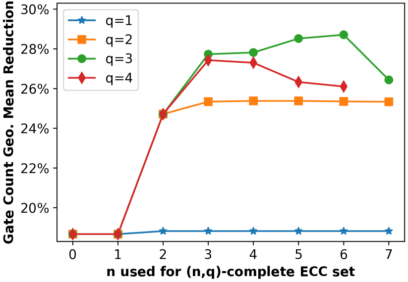
Figure 7. Optimization effectiveness with $(n,q)$-complete ECC sets for varying $n$ and $q$ after a 24-hour search timeout. For $n=0$ there are no transformations and the results match the “Quartz Preprocess” column of Table 2.

Figure 7 shows optimization effectiveness (reduction in geometric mean gate count) for varying values of $n$ and $q$, under a search timeout of 24 hours. The figure supports the tradeoff discussed above. Using too small values for $n$ and $q$ results in low effectiveness, and as we increase $n$ or $q$ effectiveness increases but then starts decreasing, as the negative impact of the large number of transformations starts outweighing their benefit. (See Table 8 for $|\mathcal{T}|$ in each configuration.) As expected, the optimal setting for $n$ and $q$ generally varies across circuits—smaller circuits tend to be better optimized with larger values of $n$ (Table 7). Still, Figure 7 shows that there are several settings that yield good overall results: $3\leq n\leq 6$ for $q=3$, and $3\leq n\leq 4$ for $q=4$.

Figure 8. Optimization effectiveness over time ($q{=}3$; $2{\leq}n{\leq}7$). For each time point, “best” computes the reduction in geometric mean gate count obtained by selecting the most effective value for $n$ at that time point for each circuit (i.e., different circuits may use different $n$’s, and the same circuit may use different $n$’s at different time points).

Figure 8 shows how the search time impacts optimization for different choices for $n$ (focusing on $q=3$). For each value of $n$, we observe a quick initial burst, followed by a gentle increase. At the end of the initial burst, effectiveness monotonically decreases as $n$ increases, for all $3\leq n\leq 6$. As time progresses the gaps diminish and eventually the order is reversed: at around 21 hours $n=6$ surpasses $n=3$. The settings $n=2$ and $n=7$ yield poor effectiveness: $n=2$ does not contain an adequate number of transformations and quickly saturates the search time, while $n=7$ contains too many transformations and progresses too slowly.

Figure 8 also shows the effectiveness of a hypothetical run constructed by taking the best setting for each circuit at each time. This “best” curve considerably outperforms the others, because the best setting for $n$ varies across circuits with different sizes.

See Appendix A for more details, including plots akin to Figure 7 and Figure 8 for each circuit.

8. Related Work

Quantum circuit compilation.

Several optimizing compilers for quantum circuits have been recently introduced and are being actively developed: Qiskit (Aleksandrowicz et al., 2019) and t$|$ket$\rangle$ (Sivarajah et al., 2020) support generic gate sets; Quilc (Skilbeck et al., 2020) is tailored to Rigetti Agave quantum processors; voqc (Hietala et al., 2021) is formally verified in Coq. CertiQ (Shi et al., 2020) is a framework for writing and verifying Qiskit compiler passes. Nam et al. (Nam et al., 2018) develop heuristics tailored to the $\{H,X,R_{z},CNOT\}$ gate set. Unlike Quartz, these systems rely on quantum-computing experts to design, implement, and verify transformations.

Quanto (Pointing et al., 2021) automatically discovers transformations by computing concrete matrix representations of circuits. It supports parameters only by considering concrete values, and unlike Quartz, it does not discover or verify symbolic transformations, which are the source of many of the challenges Quartz deals with. Quanto uses floating-point matrix equality to identify equivalence between circuits, while Quartz uses a combination of fingerprinting, SMT-based verification, the RepGen algorithm, and other pruning techniques, which are needed since symbolic parameters greatly increase the number of possible circuits in the generation procedure.

Different from the aforementioned quantum optimizers that consider circuit transformations, PyZX (Kissinger and van de Wetering, 2020) employs ZX-diagrams as an intermediate representation for quantum circuits and uses a small set of complete rewrite rules in ZX-calculus (Hadzihasanovic et al., 2018; Jeandel et al., 2018) to simplify ZX-diagrams, which are finally converted back into quantum circuits.

While our approach builds on some of the techniques developed in prior work, Quartz is the first quantum circuit optimizer that can automatically generate and verify symbolic circuit transformations for arbitrary gate sets.

Superoptimization.

Superoptimization is a compiler optimization technique originally designed to search for an optimal sequence of instructions for an input program (Massalin, 1987). Our approach to generating quantum circuit transformations by tracking equivalent classes of circuits is inspired by prior work in automatically generating peephole optimizations for the X86 instruction set (Heule et al., 2016; Bansal and Aiken, 2006) and generating graph substitutions for tensor algebra (Jia et al., 2019a; Yang et al., 2021; Wang et al., 2021).

TASO (Jia et al., 2019a) is a tensor algebra superoptimizer that optimizes computation graphs of deep neural networks using automatically generated graph substitutions. TENSAT (Yang et al., 2021) reuses the graph substitutions discovered by TASO and employs equality saturation for tensor graph superoptimization. While Quartz draws inspiration from TASO and uses a similar search procedure, it is significantly different from prior superoptimization works because it targets quantum computing, which leads to a different semantics (i.e., using complex matrices) as well as a different notion of program equivalence (i.e., up to a global phase). Verifying quantum circuit transformations therefore uses different techniques compared to other superoptimization contexts. Applying equality saturation as in TENSAT (Yang et al., 2021) for optimizing quantum circuits is an interesting avenue for future work.

9. Conclusion and Future Work

We have presented Quartz, a quantum circuit superoptimizer that automatically generates and verifies circuit transformations for arbitrary gate sets with symbolic parameters. While Quartz shows that a superoptimization-based approach to optimizing quantum circuits is practical, we believe there are many opportunities for further improvement. As discussed in Section 7.5, Quartz’s current search algorithm limits the number of transformations that can be effectively utilized. Improving the search algorithm may therefore lead to better optimization using $(n,q)$-complete ECC sets for larger values of $n$ and $q$, which may also require improving the generator. Another limitation of Quartz that suggests an opportunity for future work is that it only targets the logical circuit optimization stage and does not consider qubit mapping. Applying superoptimization to jointly optimize circuit logic and qubit mapping is both challenging and promising.

Appendix A Detailed Results

Table 7. Gate count results for the Nam gate set when using $(n,q)$-complete ECC sets with varying values of $n$ and $q$, and a search timeout of 24 hours. “Pr.” shows the result when $n=0$ or $n=1$: the ECC set is empty, so the results match the “Quartz Preprocess” column of Table 2. When $q=1$, the results are the same when $2\leq n\leq 7$.

Circuit	Orig.	Pr.	$q=1$	$q=2,n=\mbox{\tt\char 95\relax}$						$q=3,n=\mbox{\tt\char 95\relax}$						$q=4,n=\mbox{\tt\char 95\relax}$
				2	3	4	5	6	7	2	3	4	5	6	7	2	3	4	5	6
tof_3	45	39	39	35	35	35	35	35	35	35	35	35	35	35	35	35	35	35	35	35
barenco_tof_3	58	46	46	42	42	42	42	42	42	42	40	40	40	38	38	42	40	40	40	38
mod5_4	63	51	51	51	51	51	51	51	51	51	45	41	27	26	31	51	45	37	32	26
tof_4	75	63	63	55	55	55	55	55	55	55	55	55	55	55	55	55	55	55	55	55
tof_5	105	87	87	75	75	75	75	75	75	75	75	75	75	75	75	75	75	75	75	75
barenco_tof_4	114	86	86	78	78	78	78	78	78	78	72	72	72	68	68	78	72	72	72	68
mod_mult_55	119	105	105	97	94	94	94	94	94	97	92	93	93	93	94	97	92	93	93	94
vbe_adder_3	150	115	115	95	95	95	95	95	95	95	91	91	89	85	85	95	91	90	91	91
barenco_tof_5	170	126	126	114	114	114	114	114	114	114	104	104	104	98	100	114	104	104	104	102
csla_mux_3	170	164	164	160	152	152	152	152	152	160	146	148	149	154	156	160	150	148	153	153
rc_adder_6	200	174	174	154	152	152	152	152	152	154	152	152	152	154	154	154	152	152	154	156
gf2^4_mult	225	186	186	186	180	180	180	180	180	186	176	175	177	177	178	186	175	177	178	180
tof_10	255	207	207	175	175	175	175	175	175	175	175	175	175	175	175	175	175	175	175	191
mod_red_21	278	236	226	202	202	202	202	202	202	202	202	202	202	202	210	202	202	202	202	228
gf2^5_mult	347	287	287	287	279	279	279	279	279	287	273	273	273	277	279	287	277	277	279	283
csum_mux_9	420	308	308	308	308	308	308	308	308	308	280	280	280	272	302	308	280	280	305	307
qcla_com_7	443	349	347	293	293	293	293	293	293	293	289	288	288	292	339	293	289	288	321	347
barenco_tof_10	450	326	326	294	294	294	294	294	294	294	268	271	271	262	316	294	268	275	298	324
gf2^6_mult	495	401	401	401	391	391	391	391	391	401	381	383	386	391	393	401	386	391	391	401
qcla_adder_10	521	450	450	416	414	414	414	414	414	416	407	408	408	422	444	416	408	414	436	450
gf2^7_mult	669	543	543	543	531	531	531	531	531	543	517	519	529	531	539	543	524	530	537	543
gf2^8_mult	883	703	703	703	703	703	703	703	703	703	690	703	703	703	703	703	703	703	703	703
qcla_mod_7	884	727	727	657	657	657	657	657	657	657	654	651	677	719	727	657	655	697	725	727
adder_8	900	732	732	644	640	640	640	640	644	644	638	634	688	724	732	644	634	706	730	732
gf2^9_mult	1095	879	879	879	877	869	869	877	877	879	857	856	870	873	879	879	857	871	879	879
gf2^10_mult	1347	1062	1062	1062	1062	1058	1058	1058	1058	1062	1030	1049	1052	1060	1062	1062	1061	1058	1062	1062

Table 8. Metrics for Quartz’s generator, when generating $(n,q)$-complete ECC sets for $2\leq n\leq 7$ and $1\leq q\leq 4$ for the Nam gate set. $|\mathcal{T}|$ is the resulting number of transformations. The characteristics (see definition in Section 3.3) for $q=1,2,3,4$ are 7, 16, 27, 40, respectively.

	$|\mathcal{T}|$				Verification Time (s)				Total Time (s)
$n$	$q=1$	$q=2$	$q=3$	$q=4$	$q=1$	$q=2$	$q=3$	$q=4$	$q=1$	$q=2$	$q=3$	$q=4$
2	14	38	62	78	0.5	0.7	1.2	2.5	0.5	0.7	1.3	2.8
3	14	90	196	208	0.8	1.3	2.6	7.8	0.8	1.5	3.7	12.0
4	44	332	1,304	2,988	1.1	2.3	8.5	48.0	1.2	3.8	21.4	118.3
5	78	1,334	8,002	27,942	1.5	8.8	49.5	917.0	1.6	19.2	174.7	2,452.0
6	120	5,794	56,152	273,532	1.9	52.5	370.3	5,802.6	2.2	138.9	1,400.4	19,448.0
7	164	21,824	379,864	–$\dagger$	2.3	71.8	2,673.6	–$\dagger$	2.8	222.9	10,461.2	–$\dagger$

• We were unable to generate a $(7,4)$-complete ECC set using $512\text{\,}\mathrm{G}\mathrm{B}$ of RAM.

Table 7 shows the final gate count for each circuit for varying $n$ and $q$ after a 24-hour search timeout, with the best results of each circuit highlighted. Interestingly, $q=3$ with $3\leq n\leq 6$ covers the best optimization results for all circuits obtained among all configurations considered in the table. As circuits are sorted in the order of original size in the table, we can see that when $q=3$, small circuits tend to be better optimized with larger values of $n$, and larger circuits tend to be better optimized with smaller values of $n$.

Table 8 shows the run times of the entire generation procedure, and also the time out of that spent in verification, for each of the ECC set used in Table 7. The table also lists the number of resulting circuit transformations $|\mathcal{T}|$ for each $n$ and $q$, and the characteristic for each $q$ (see definition in Section 3.3).

Figures 9, 10, 11, 12, 13, 14, 15, 16, 17, 18, 19, 20, 21, 22, 23, 24, 25, 26, 27, 28, 29, 30, 31, 32, 33 and 34 show plots akin to Figure 7 and Figure 8 for each circuit. In each figure, the left plot shows the optimization result with $(n,q)$-complete ECC sets for varying $n$ and $q$ after a 24-hour search timeout. The right plot shows the optimization result over time for $q=3$ and $2\leq n\leq 7$. Each 24-hour result on the right plot corresponds to a green round marker ($q=3$) on the left plot.

Among these figures, Figure 23 shows the median run for mod5_4. The median run is defined to be the run with the final gate count being the median of the 7 runs. We present the results of all 7 runs for mod5_4 for $q=3$ and $3\leq n\leq 7$ in Figure 35.

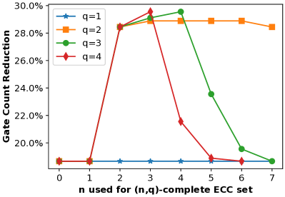
Figure 9. adder_8 (900 gates).

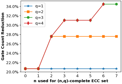
Figure 10. barenco_tof_3 (58 gates).

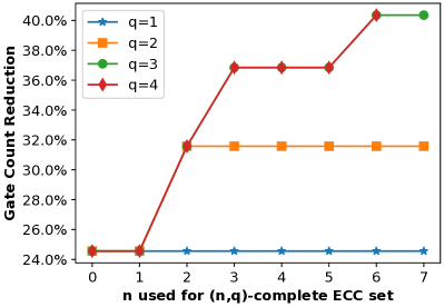
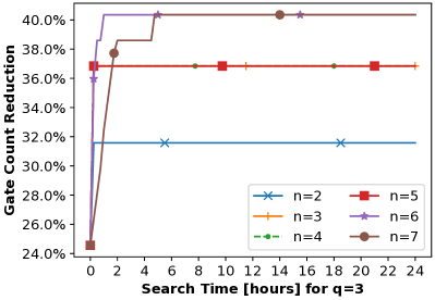
Figure 11. barenco_tof_4 (114 gates).

Figure 12. barenco_tof_5 (170 gates).

Figure 13. barenco_tof_10 (450 gates).

Figure 14. csla_mux_3 (170 gates).

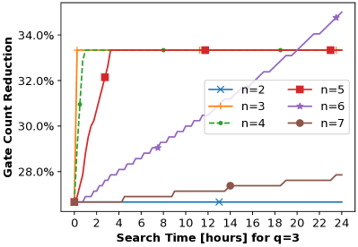
Figure 15. csum_mux_9 (420 gates).

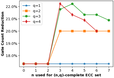
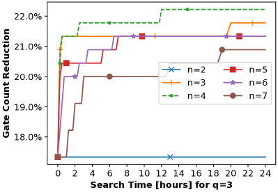
Figure 16. gf2^4_mult (225 gates).

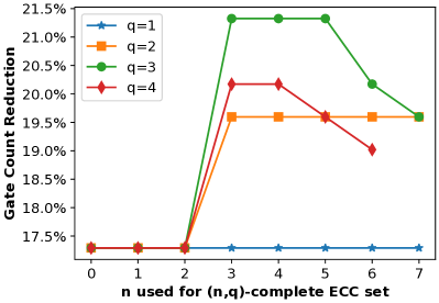
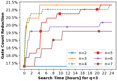
Figure 17. gf2^5_mult (347 gates).

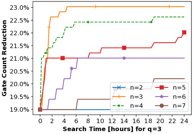
Figure 18. gf2^6_mult (495 gates).

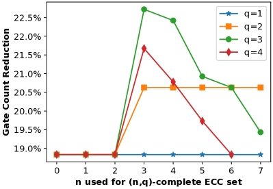
Figure 19. gf2^7_mult (669 gates).

Figure 20. gf2^8_mult (883 gates).

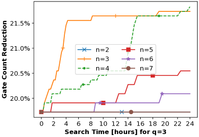
Figure 21. gf2^9_mult (1095 gates).

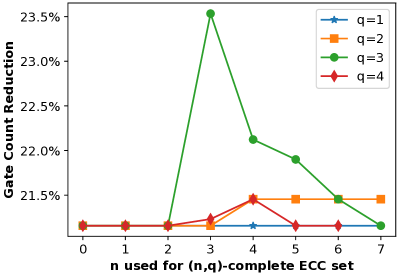
Figure 22. gf2^10_mult (1347 gates).

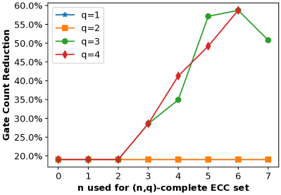
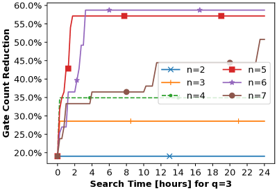
Figure 23. mod5_4 (63 gates).

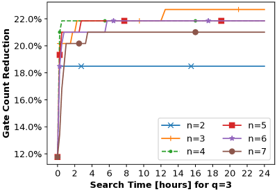
Figure 24. mod_mult_55 (119 gates).

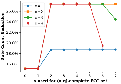
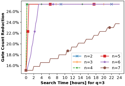
Figure 25. mod_red_21 (278 gates).

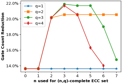
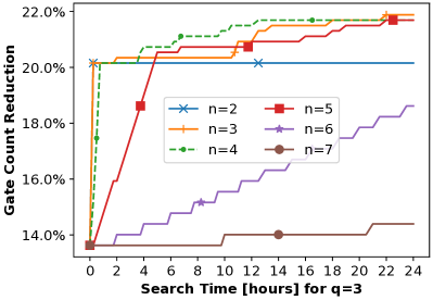
Figure 26. qcla_adder_10 (521 gates).

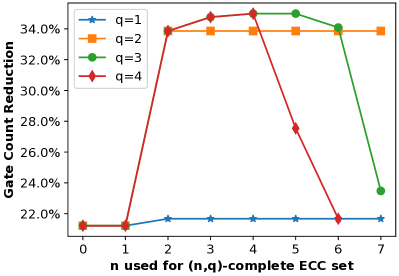
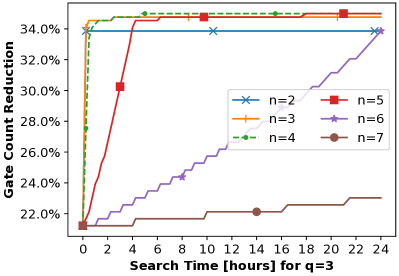
Figure 27. qcla_com_7 (443 gates).

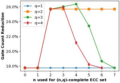
Figure 28. qcla_mod_7 (884 gates).

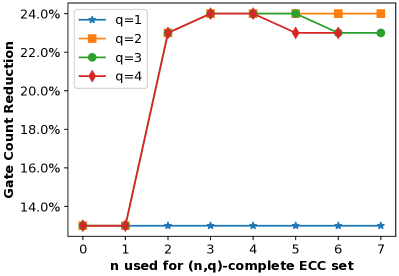
Figure 29. rc_adder_6 (200 gates).

Figure 30. tof_3 (45 gates).

Figure 31. tof_4 (75 gates).

Figure 32. tof_5 (105 gates).

Figure 33. tof_10 (255 gates).

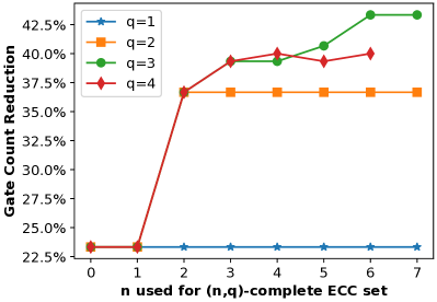
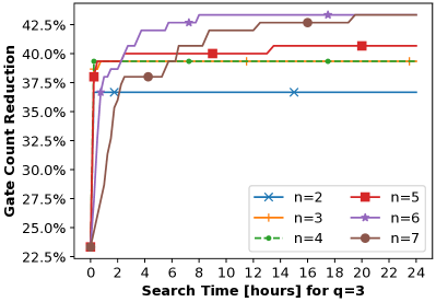
Figure 34. vbe_adder_3 (150 gates).

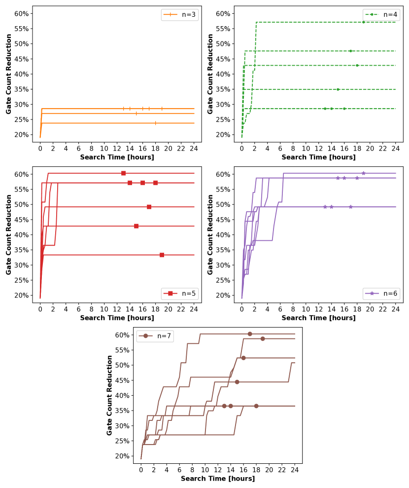
Figure 35. 7 runs of mod5_4 with a $(n,3)$-complete ECC set for each $3\leq n\leq 7$. Each marker denotes one run. For example, the three markers on the 57.1%-reduction line of $n=5$ show three runs resulting in 27 gates after 24 hours.

References

- (1)
- qis (2021a) 2021a. Qiskit ConsolidateBlocks. https://qiskit.org/documentation/stubs/qiskit.transpiler.passes.ConsolidateBlocks.html.
- qis (2021b) 2021b. Qiskit Optimize1qGates. https://qiskit.org/documentation/stubs/qiskit.transpiler.passes.Optimize1qGates.html.
- rig (2021) 2021. Rigetti Gates. https://pyquil-docs.rigetti.com/en/v2.7.0/apidocs/gates.html.
- qua (2022) 2022. The Quartz Quantum Circuit SuperOptimizer. https://github.com/quantum-compiler/quartz.
- Aleksandrowicz et al. (2019) Gadi Aleksandrowicz, Thomas Alexander, Panagiotis Barkoutsos, Luciano Bello, Yael Ben-Haim, David Bucher, Francisco Jose Cabrera-Hernández, Jorge Carballo-Franquis, Adrian Chen, Chun-Fu Chen, Jerry M. Chow, Antonio D. Córcoles-Gonzales, Abigail J. Cross, Andrew Cross, Juan Cruz-Benito, Chris Culver, Salvador De La Puente González, Enrique De La Torre, Delton Ding, Eugene Dumitrescu, Ivan Duran, Pieter Eendebak, Mark Everitt, Ismael Faro Sertage, Albert Frisch, Andreas Fuhrer, Jay Gambetta, Borja Godoy Gago, Juan Gomez-Mosquera, Donny Greenberg, Ikko Hamamura, Vojtech Havlicek, Joe Hellmers, Łukasz Herok, Hiroshi Horii, Shaohan Hu, Takashi Imamichi, Toshinari Itoko, Ali Javadi-Abhari, Naoki Kanazawa, Anton Karazeev, Kevin Krsulich, Peng Liu, Yang Luh, Yunho Maeng, Manoel Marques, Francisco Jose Martín-Fernández, Douglas T. McClure, David McKay, Srujan Meesala, Antonio Mezzacapo, Nikolaj Moll, Diego Moreda Rodríguez, Giacomo Nannicini, Paul Nation, Pauline Ollitrault, Lee James O’Riordan, Hanhee Paik, Jesús Pérez, Anna Phan, Marco Pistoia, Viktor Prutyanov, Max Reuter, Julia Rice, Abdón Rodríguez Davila, Raymond Harry Putra Rudy, Mingi Ryu, Ninad Sathaye, Chris Schnabel, Eddie Schoute, Kanav Setia, Yunong Shi, Adenilton Silva, Yukio Siraichi, Seyon Sivarajah, John A. Smolin, Mathias Soeken, Hitomi Takahashi, Ivano Tavernelli, Charles Taylor, Pete Taylour, Kenso Trabing, Matthew Treinish, Wes Turner, Desiree Vogt-Lee, Christophe Vuillot, Jonathan A. Wildstrom, Jessica Wilson, Erick Winston, Christopher Wood, Stephen Wood, Stefan Wörner, Ismail Yunus Akhalwaya, and Christa Zoufal. 2019. Qiskit: An Open-source Framework for Quantum Computing. https://doi.org/10.5281/zenodo.2562111
- Amy et al. (2014) Matthew Amy, Dmitri Maslov, and Michele Mosca. 2014. Polynomial-Time T-Depth Optimization of Clifford+T Circuits Via Matroid Partitioning. IEEE Transactions on Computer-Aided Design of Integrated Circuits and Systems 33, 10 (2014), 1476–1489. https://doi.org/10.1109/TCAD.2014.2341953
- Bansal and Aiken (2006) Sorav Bansal and Alex Aiken. 2006. Automatic Generation of Peephole Superoptimizers. SIGOPS Oper. Syst. Rev. 40, 5 (Oct. 2006), 394–403. https://doi.org/10.1145/1168917.1168906
- Barrett et al. (2011) Clark W. Barrett, Christopher L. Conway, Morgan Deters, Liana Hadarean, Dejan Jovanovic, Tim King, Andrew Reynolds, and Cesare Tinelli. 2011. CVC4. In Computer Aided Verification - 23rd International Conference, CAV 2011, Snowbird, UT, USA, July 14-20, 2011. Proceedings (Lecture Notes in Computer Science, Vol. 6806), Ganesh Gopalakrishnan and Shaz Qadeer (Eds.). Springer, 171–177. https://doi.org/10.1007/978-3-642-22110-1_14
- Cimatti et al. (2017) Alessandro Cimatti, Alberto Griggio, Ahmed Irfan, Marco Roveri, and Roberto Sebastiani. 2017. Satisfiability Modulo Transcendental Functions via Incremental Linearization. In Automated Deduction - CADE 26 - 26th International Conference on Automated Deduction, Gothenburg, Sweden, August 6-11, 2017, Proceedings (Lecture Notes in Computer Science, Vol. 10395), Leonardo de Moura (Ed.). Springer, 95–113. https://doi.org/10.1007/978-3-319-63046-5_7
- de Moura and Bjørner (2008) Leonardo de Moura and Nikolaj Bjørner. 2008. Z3: An Efficient SMT Solver. In Tools and Algorithms for the Construction and Analysis of Systems, 14th International Conference, TACAS 2008, Held as Part of the Joint European Conferences on Theory and Practice of Software, ETAPS 2008, Budapest, Hungary, March 29-April 6, 2008. Proceedings (Lecture Notes in Computer Science, Vol. 4963), C. R. Ramakrishnan and Jakob Rehof (Eds.). Springer, 337–340. https://doi.org/10.1007/978-3-540-78800-3_24
- Ding et al. (2018) Yongshan Ding, Adam Holmes, Ali Javadi-Abhari, Diana Franklin, Margaret Martonosi, and Frederic T. Chong. 2018. Magic-State Functional Units: Mapping and Scheduling Multi-Level Distillation Circuits for Fault-Tolerant Quantum Architectures. In 51st Annual IEEE/ACM International Symposium on Microarchitecture, MICRO 2018, Fukuoka, Japan, October 20-24, 2018. IEEE Computer Society, 828–840. https://doi.org/10.1109/MICRO.2018.00072
- Dumitrescu et al. (2018) Eugene F Dumitrescu, Alex J McCaskey, Gaute Hagen, Gustav R Jansen, Titus D Morris, T Papenbrock, Raphael C Pooser, David Jarvis Dean, and Pavel Lougovski. 2018. Cloud quantum computing of an atomic nucleus. Physical review letters 120, 21 (2018), 210501.
- Hadzihasanovic et al. (2018) Amar Hadzihasanovic, Kang Feng Ng, and Quanlong Wang. 2018. Two Complete Axiomatisations of Pure-State Qubit Quantum Computing. In Proceedings of the 33rd Annual ACM/IEEE Symposium on Logic in Computer Science (Oxford, United Kingdom) (LICS ’18). Association for Computing Machinery, New York, NY, USA, 502–511. https://doi.org/10.1145/3209108.3209128
- Heule et al. (2016) Stefan Heule, Eric Schkufza, Rahul Sharma, and Alex Aiken. 2016. Stratified Synthesis: Automatically Learning the X86-64 Instruction Set. In Proceedings of the 37th ACM SIGPLAN Conference on Programming Language Design and Implementation (Santa Barbara, CA, USA) (PLDI ’16). Association for Computing Machinery, New York, NY, USA, 237–250. https://doi.org/10.1145/2908080.2908121
- Hietala et al. (2021) Kesha Hietala, Robert Rand, Shih-Han Hung, Xiaodi Wu, and Michael Hicks. 2021. A Verified Optimizer for Quantum Circuits. Proc. ACM Program. Lang. 5, POPL, Article 37 (Jan. 2021), 29 pages. https://doi.org/10.1145/3434318
- Jeandel et al. (2018) Emmanuel Jeandel, Simon Perdrix, and Renaud Vilmart. 2018. A Complete Axiomatisation of the ZX-Calculus for Clifford+T Quantum Mechanics. In Proceedings of the 33rd Annual ACM/IEEE Symposium on Logic in Computer Science (Oxford, United Kingdom) (LICS ’18). Association for Computing Machinery, New York, NY, USA, 559–568. https://doi.org/10.1145/3209108.3209131
- Jia et al. (2019a) Zhihao Jia, Oded Padon, James Thomas, Todd Warszawski, Matei Zaharia, and Alex Aiken. 2019a. TASO: Optimizing Deep Learning Computation with Automatic Generation of Graph Substitutions. In Proceedings of the 27th ACM Symposium on Operating Systems Principles (Huntsville, Ontario, Canada) (SOSP ’19). Association for Computing Machinery, New York, NY, USA, 47–62. https://doi.org/10.1145/3341301.3359630
- Jia et al. (2019b) Zhihao Jia, James Thomas, Todd Warzawski, Mingyu Gao, Matei Zaharia, and Alex Aiken. 2019b. Optimizing DNN Computation with Relaxed Graph Substitutions. In Proceedings of the 2nd Conference on Systems and Machine Learning (SysML’19).
- Kissinger and van de Wetering (2019) Aleks Kissinger and John van de Wetering. 2019. Reducing T-count with the ZX-calculus. arXiv preprint arXiv:1903.10477 (2019).
- Kissinger and van de Wetering (2020) Aleks Kissinger and John van de Wetering. 2020. PyZX: Large Scale Automated Diagrammatic Reasoning. Electronic Proceedings in Theoretical Computer Science 318 (may 2020), 229–241. https://doi.org/10.4204/eptcs.318.14
- Koenig et al. (2021) Jason R. Koenig, Oded Padon, and Alex Aiken. 2021. Adaptive restarts for stochastic synthesis. In PLDI ’21: 42nd ACM SIGPLAN International Conference on Programming Language Design and Implementation, Virtual Event, Canada, June 20-25, 2021, Stephen N. Freund and Eran Yahav (Eds.). ACM, 696–709. https://doi.org/10.1145/3453483.3454071
- Massalin (1987) Henry Massalin. 1987. Superoptimizer: A Look at the Smallest Program (ASPLOS II). IEEE Computer Society Press, Washington, DC, USA, 122–126. https://doi.org/10.1145/36206.36194
- Nam et al. (2018) Yunseong Nam, Neil J Ross, Yuan Su, Andrew M Childs, and Dmitri Maslov. 2018. Automated optimization of large quantum circuits with continuous parameters. npj Quantum Information 4, 1 (2018), 1–12.
- Nielsen and Chuang (2001) M. Nielsen and I. Chuang. 2001. Quantum Computation and Quantum Information. Cambridge University Press.
- Pointing et al. (2021) Jessica Pointing, Oded Padon, Zhihao Jia, Henry Ma, Auguste Hirth, Jens Palsberg, and Alex Aiken. 2021. Quanto: Optimizing Quantum Circuits with Automatic Generation of Circuit Identities. arXiv:2111.11387 (2021). https://doi.org/10.48550/arXiv.2111.11387
- Reagor et al. (2018) Matthew Reagor, Christopher B. Osborn, Nikolas Tezak, Alexa Staley, Guenevere Prawiroatmodjo, Michael Scheer, Nasser Alidoust, Eyob A. Sete, Nicolas Didier, Marcus P. da Silva, and et al. 2018. Demonstration of universal parametric entangling gates on a multi-qubit lattice. Science Advances 4, 2 (Feb 2018). https://doi.org/10.1126/sciadv.aao3603
- Shi et al. (2020) Yunong Shi, Runzhou Tao, Xupeng Li, Ali Javadi-Abhari, Andrew W. Cross, Frederic T. Chong, and Ronghui Gu. 2020. CertiQ: A Mostly-automated Verification of a Realistic Quantum Compiler. arXiv:1908.08963 [quant-ph]
- Sivarajah et al. (2020) Seyon Sivarajah, Silas Dilkes, Alexander Cowtan, Will Simmons, Alec Edgington, and Ross Duncan. 2020. t—ket⟩: a retargetable compiler for NISQ devices. Quantum Science and Technology 6, 1 (Nov 2020), 014003. https://doi.org/10.1088/2058-9565/ab8e92
- Skilbeck et al. (2020) Mark Skilbeck, Eric Peterson, appleby, Erik Davis, Peter Karalekas, Juan M. Bello-Rivas, Daniel Kochmanski, Zach Beane, Robert Smith, Andrew Shi, Cole Scott, Adam Paszke, Eric Hulburd, Matthew Young, Aaron S. Jackson, BHAVISHYA, M. Sohaib Alam, Wilfredo Velázquez-Rodríguez, c. b. osborn, fengdlm, and jmackeyrigetti. 2020. rigetti/quilc: v1.21.0. https://doi.org/10.5281/zenodo.3967926
- Wang et al. (2021) Haojie Wang, Jidong Zhai, Mingyu Gao, Zixuan Ma, Shizhi Tang, Liyan Zheng, Yuanzhi Li, Kaiyuan Rong, Yuanyong Chen, and Zhihao Jia. 2021. PET: Optimizing Tensor Programs with Partially Equivalent Transformations and Automated Corrections. In 15th USENIX Symposium on Operating Systems Design and Implementation (OSDI 21). 37–54.
- Wu et al. (2021) Xin-Chuan Wu, Dripto M. Debroy, Yongshan Ding, Jonathan M. Baker, Yuri Alexeev, Kenneth R. Brown, and Frederic T. Chong. 2021. TILT: Achieving Higher Fidelity on a Trapped-Ion Linear-Tape Quantum Computing Architecture. In IEEE International Symposium on High-Performance Computer Architecture, HPCA 2021, Seoul, South Korea, February 27 - March 3, 2021. IEEE, 153–166. https://doi.org/10.1109/HPCA51647.2021.00023
- Xu et al. (2022a) Mingkuan Xu, Zikun Li, Oded Padon, Sina Lin, Jessica Pointing, Auguste Hirth, Henry Ma, Jens Palsberg, Alex Aiken, Umut A. Acar, and Zhihao Jia. 2022a. Artifact for PLDI 2022 paper: Quartz: Superoptimization of quantum circuits. https://doi.org/10.5281/zenodo.6508992
- Xu et al. (2022b) Mingkuan Xu, Zikun Li, Oded Padon, Sina Lin, Jessica Pointing, Auguste Hirth, Henry Ma, Jens Palsberg, Alex Aiken, Umut A. Acar, and Zhihao Jia. 2022b. Quartz: Superoptimization of quantum circuits. In Proceedings of the 43rd ACM SIGPLAN International Conference on Programming Language Design and Implementation (PLDI ’22), June 13–17, 2022, San Diego, CA, USA. ACM. https://doi.org/10.1145/3519939.3523433
- Yang et al. (2021) Yichen Yang, Phitchaya Phothilimthana, Yisu Wang, Max Willsey, Sudip Roy, and Jacques Pienaar. 2021. Equality Saturation for Tensor Graph Superoptimization. In Proceedings of Machine Learning and Systems, A. Smola, A. Dimakis, and I. Stoica (Eds.), Vol. 3. 255–268.