Mathematics of Floating 3D Printed Objects

Abstract.

We explore the stability of floating objects through mathematical modeling and experimentation. Our models are based on standard ideas of center of gravity, center of buoyancy, and Archimedes’ Principle. We investigate a variety of floating shapes with two-dimensional cross sections and identify analytically and/or computationally a potential energy landscape that helps identify stable and unstable floating orientations. We compare our analyses and computations to experiments on floating objects designed and created through 3D printing. In addition to our results, we provide code for testing the floating configurations for new shapes, as well as giving details of the methods for 3D printing the objects. The paper includes conjectures and open problems for further study.

1. Introduction

Interest in the dynamics of icebergs has been driven by the desire to describe various natural phenomena (including their rolling) as well as practical considerations associated with shipping and protection of offshore structures in arctic environments. Allaire’s [Allaire1972] study of iceberg stability was motivated by the need to assess mitigation strategies, such as towing of icebergs, to reduce threats posed by icebergs to offshore structures. Allaire identified readily-identifiable above-water characteristics, such as the ratio of waterline width to above-water height, to estimate stability for a menagerie of iceberg shapes – Blocky, Drydock, Dome, Pinnacled, Tabular, Growler. Bailey [Bailey1994], motivated by similar concerns, examined stability of icebergs in terms of rolling frequency. The potential for iceberg stability considerations to be dynamic even in calm water due to underwater melting/dissolution was considered by Deriabyn & Hjorth [DH2009]. They were also interested to identify what practical, above-water, observations could be made to predict stability changes driven by underwater changes in iceberg morphology.

Ship design and the design of other man-made floating objects has no doubt driven much scientific and technical work in this field. We make no attempt to review this literature but interested readers may find resources in the work of Mégel & Kliava [MK2010] and Wilczynski & Diehl [WD1995]. Historically speaking, scientific thought on this dates back to Archimedes (c. 287–212/211 B.C.). See for example Rorres [Rorres2004], a fascinating article on the original work of Archimedes and extensions thereof.

Whereas icebergs and ships are complex three dimensional floating objects, the floating objects that are the focus of the present work are those whose configurations can effectively be characterized in two-dimensions. Specifically, we shall consider ‘long’ objects whose cross sections are constant for the full length of the object. Such shapes have been the focus of popular online Apps, such as Iceberger [Iceberger] and the remixed version [IcebergerRemix]. These effective two-dimensional floating objects have proven to be mathematically tractable yet rich in observable phenomena. Prediction of the stable orientations for a long beam with square-cross section and uniform density, for example, was considered by Reid [Reid1963]. Depending on the ratio of the density of the object to the density of the fluid any rotation of the square can be a stable floating orientation (i.e. any orientation from flat side up to corner up). This configuration has been recently revisited both experimentally and analytically by Feigel and Fuzailov [FF2021]. These authors validated experimentally that for a small range of density ratios near $0.25$ (and also similarly near $0.75$) the full range of stable orientations can be realized. Another view of this which we discuss in more detail in our work is that owing to the four-fold symmetry of the square, there can be either four or eight stable orientations of the floating square depending on the density ratio. We explore how these results change for what we denote as ‘off-center’ squares.

The case of a long ‘floating plank’ of rectangular cross section was the focus of work by Delbourgo [Delbourgo1987]. Here, in addition to the density ratio, another parameter – the aspect ratio of the rectangle – appears. Delbourgo identified in this density ratio vs. aspect ratio space the existence of six characteristic floating configurations in terms of (1) long side up or short side up, (2) top side parallel or not parallel to the waterline, and (2) the number of submerged vertices. Further studies have explored other cross sectional shapes and investigated details of the breaking of left-right symmetries of the floating shapes as the density ratio is varied (e.g. see Erdös, Schibler, & Herndon [Erdos_etal1992_part1] for square and equilateral triangle cross sections and Erdös, Schibler, & Herndon [Erdos_etal1992_part2] for the three-dimensional shapes of the cube, octahedron, and decahedron). Work in this area has focused on homogeneous objects with uniform density. We shall relax this assumption in our present work to include some special classes of non-uniform density in which the center of gravity of the square no longer resides at its centroid (cf. Definition 2.1).

An excellent review of many important mathematical ideas – Archimedes’ Principle, Center of Gravity, Center of Buoyancy, and the notion of Metacenter – related to floating objects is the work of Gilbert [Gilbert1991]. One particularly useful concept is that of the potential energy of floating objects. Gilbert shows that if one can compute the potential energy landscape as a function of all possible orientations of the object one can identify stable floating configurations by the locations of local minima of the potential energy function. This is one of the main objectives of our computations as we then use this to identify stable orientations.

The present work shares some of the spirit of the paper by Feigel and Fuzailov [FF2021] to revisit these questions both theoretically and experimentally. Our experiments, however, are conducted with 3D printed shapes. While some of our theoretical effort has been on objects with square cross section, our methodology is motivated by the recognition that 3D printing offers the opportunity to float objects whose cross sections are effectively limited only by ones own creativity in defining new shapes. An example shape we analyze is the ‘Mason M’ shown in Figure 1.

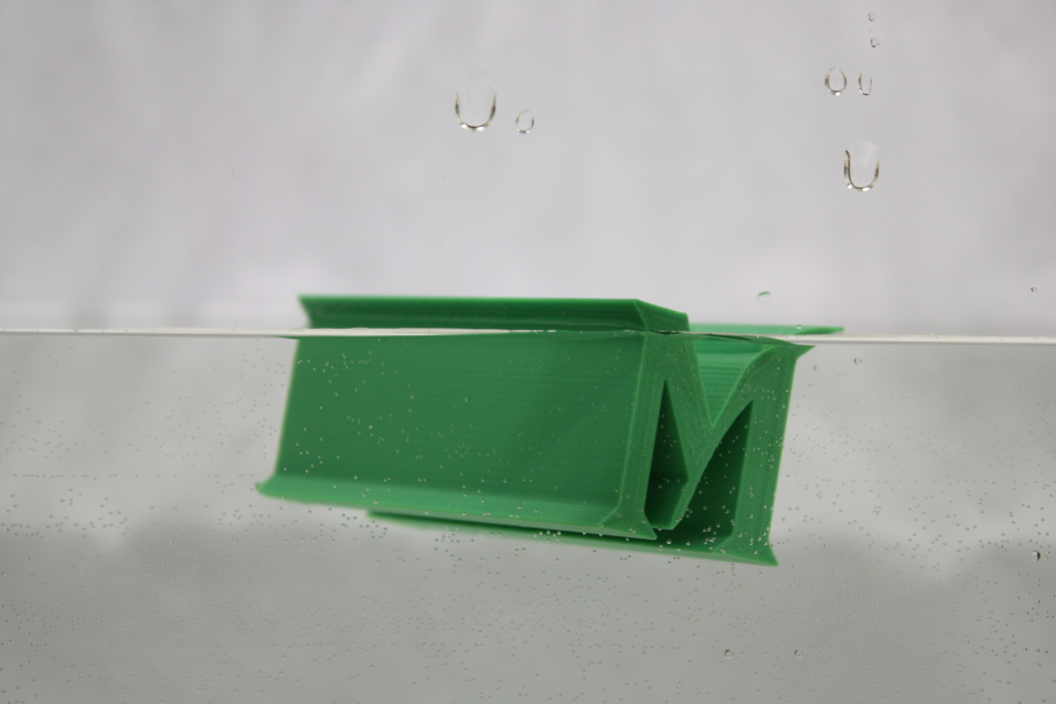
Figure 1. The floating Mason M.

The new contributions we make here are (1) predicting floating configurations of an object with square cross section when the center of gravity is not at the object’s centroid, (2) predicting floating configurations for objects of general two-dimensional polygonal cross section, and (3) verifying the predictions of (1) and (2) as well as classical ones for objects of square cross section with experiments conducted with 3D printed objects.

This paper is organized as follows. In Section 2, we introduce definitions and terminology, outline prior results for long floating objects of uniform density with square cross section, and state our analytical results for the case of long floating objects with square cross section with non-uniform density. In Section LABEL:sec:3DPrinting we give a detailed description of how to 3D print floating objects. This section contains sufficient details and accompanying code so that interested readers would be able to print their own objects and perform their own experiments. Note that we have additionally provided codes and files in a GitHub repository [GITHUB]. In Section LABEL:sec:Experiments we describe how we obtain experimental results on our 3D printed floating objects. In Section LABEL:sec:compexp we describe our code for computing stable floating configurations for objects with general polygonal cross sections. In Section LABEL:sec:Results we describe the results of our floating experiments and relate them to our theoretical results for several cases involving square cross sections and a selected case of a nontrivial cross section. In Section LABEL:sec:conclusion we give our conclusions and discuss some open problems.

2. Mathematical Models for Floating Objects

2.1. Definitions

In this section, we give some basic definitions and concepts that will be needed for the remainder of our analysis.

Definition 2.1 (Center of Gravity).

If the mass distribution is given by a continuous density function of $\rho(x,y,z)$ within a domain $\Omega$, then the center of gravity can be obtained by

$$(G_{x},G_{y},G_{z})=\frac{1}{M_{\rm{obj}}}\iiint_{\Omega}(x,y,z)\,\rho(x,y,z)\;dV\;,$$

where $M_{\rm{obj}}$ is the object’s mass. In the case of uniform density, i.e. $\rho$ is a constant independent of $x,y$ and $z$, the center of gravity is called the centroid.

For a long object of length $L$ with uniform cross section, with uniform density in the long direction, i.e. $\rho(x,y,z)=\rho(x,y)$ is independent of $z$, the center of gravity is given by

$$\vec{G}=(G_{x},G_{y})=\frac{L}{M_{\rm{obj}}}\iint_{\Omega}(x,y)\rho(x,y)\;dA$$

with $G_{z}=L/2$ (relative to one end of the object).

Lemma 2.2.

For an object of length $L$ with a polygonal cross-section with uniform constant density $\rho$, we can compute the area and center of gravity as sums involving only the vertices of the polygon. In particular, let

$$\{(x_{1},y_{1}),\dots,(x_{N},y_{N}),(x_{1},y_{1})\}$$

be the vertices of the cross section polygon, oriented counterclockwise. Then the mass of the object is

$$M_{\rm{obj}}=\rho LA\;,$$

where the area $A$ of the polygon of cross section is given by

(2.1) $$A=\frac{1}{2}\sum_{k=1}^{N}(x_{k}+x_{k+1})(y_{k+1}-y_{k})\;,$$

a result also known as the shoelace formula, and the center of gravity $\vec{G}=(G_{x},G_{y})$ is given by

(2.2) $$G_{x} = \frac{1}{6A}\sum_{k=1}^{N}(x^{2}_{k}+x_{k}x_{k+1}+x^{2}_{k+1})(y_{k+1}-y_{k})$$

$$G_{y} = \frac{1}{6A}\sum_{k=1}^{N}-(y^{2}_{k}+y_{k}y_{k+1}+y^{2}_{k+1})(x_{k+1}-x_{k})\,.$$

Proof.

According to Green’s theorem

$$\iint_{\Omega}\left(\frac{dg}{dx}-\frac{df}{dy}\right)\;dA=\oint_{d\Omega}\,f\;dx+g\;dy,$$

Choose $(f,g)=(0,x)$ so that $\frac{dg}{dx}-\frac{df}{dy}=1$. We can parametrize the line segment between $(x_{k},y_{k})$ and $(x_{k+1},y_{k+1})$ by $(x,y)=(1-t)(x_{k},y_{k})+t(x_{k+1},y_{k+1})$ where $t\in(0,1)$. For this line segment, we get $dx=(x_{k+1}-x_{k})dt$ and $dy=(y_{k+1}-y_{k})dt$. Now we evaluate the integral from Green’s theorem:

$$\int_{0}^{1}x\;dy = \int_{0}^{1}(x_{k}+t(x_{k+1}-x_{k}))(y_{k+1}-y_{k})\;dt$$

$$= x_{k}(y_{k+1}-y_{k})+\frac{1}{2}(x_{k+1}-x_{k})(y_{k+1}-y_{k})$$

$$= \frac{1}{2}(x_{k+1}+x_{k})(y_{k+1}-y_{k})\;.$$

Now we use this to calculate the full area:

$$A=\iint_{\Omega}\;dA=\oint_{d\Omega}x\;dy=\frac{1}{2}\sum_{k=1}^{N}(x_{k+1}+x_{k})(y_{k+1}-y_{k})\;.$$

Now we turn our attention to the calculation of $G_{x}$. We use Green’s theorem but this time with $(f,g)=(0,x^{2}/2)$ in order to satisfy $\frac{dg}{dx}-\frac{df}{dy}=x$. Again for the line segment from $(x_{k},y_{k})$ to $(x_{k+1},y_{k+1})$ we get

$$\iint_{\Omega}xdA = \oint_{d\Omega}\frac{x^{2}}{2}\;dy$$

$$= \frac{1}{2}\int_{0}^{1}(x_{k}+t(x_{k+1}-x_{k}))^{2}(y_{k+1}-y_{k})\;dt$$

$$= \frac{1}{6}(x_{k}^{2}+x_{k}x_{k+1}+x_{k+1}^{2})(y_{k+1}-y_{k})\;.$$

Since $\rho$ is constant, we get that $G_{x}$ is equal to $\rho L/M_{\rm obj}$ times this integral, but $M_{\rm obj}=\rho LA$, and this gives the factor of $1/A$ written in the formula above. In a similar way, using Green’s theorem with $(f,g)=(-y^{2}/2,0)$, we get

$$\iint_{\Omega}ydA=-\frac{1}{6}(y_{k}^{2}+y_{k}y_{k+1}+y_{k+1}^{2})(x_{k+1}-x_{k})\;.$$

This gives the equation for $G_{y}$ stated above. ∎

The proof above relies on Green’s theorem, but there are other ways to derive this formula, such as dividing the object into triangles or trapezoids, and combining the corresponding triangle or trapezoid area and center of gravity formulas.

Definition 2.3 (Buoyancy).

Buoyancy is a force exerted on an object that is wholly or partially submerged in a fluid. The magnitude of this force is equal to the weight of the displaced fluid. Buoyancy relates to the density of the fluid, the volume of the displaced fluid, and the gravitational field; it is independent of the mass and density of the immersed object. The buoyancy force acts vertically upward at the centroid of the displaced volume. The center of buoyancy is given by

(2.3) $$(B_{x},B_{y},B_{z})=\frac{1}{V_{\rm{sub}}}\iiint_{\Omega_{\rm{sub}}}(x,y,z)\;dV,$$

where $V_{\rm{sub}}$ is the submerged volume of the object, and $\Omega_{\rm{sub}}$ is the submerged domain. Like in the case of center of gravity, in the uniform cross section case $B_{z}=L/2$. We use the notation $\vec{B}=(B_{x},B_{y})$. Note that $\vec{B}$ is the centroid of the submerged domain.

We now state one of the major results necessary for understanding floating objects.

Theorem 2.4 (Archimedes’ Principle).

The upward buoyant force exerted on an object wholly or partially submerged is equal to the weight of the displaced fluid. In the absence of other forces, such as surface tension, this can be expressed in the force balance as

(2.4) $$M_{\rm{obj}}g = \rho_{\rm{f}}V_{\rm{sub}}g,$$

where $g$ is acceleration due to gravity, $\rho_{\rm{f}}$ is the density of the fluid, and $V_{\rm{sub}}$ is the submerged volume of the object.

Observe that (2.4) represents a balanced (net zero) equation of competing forces with the left terms representing gravitational force and right term representing the opposing force of buoyancy. Note that if the object has uniform density, then the mass of the object can be written as $M_{\rm{obj}}=\rho_{\rm{obj}}V_{\rm{obj}}$. In this case, it follows that

(2.5) $$\frac{V_{\rm{sub}}}{V_{\rm{obj}}} = \frac{\rho_{\rm{obj}}}{\rho_{\rm{f}}}.$$

For our purposes, Archimedes’ Principle determines the appropriate waterline intersections defining a submerged volume whose value relative to the total volume matches the appropriate density ratio. However, it is important to note that satisfying Archimedes’ Principle is not a sufficient condition for determining a stable equilibrium. An equilibrium orientation of a floating body occurs when the center of gravity and the center of buoyancy are vertically aligned. If $\vec{G}$ lies directly below $\vec{B}$ the equilibrium is stable, whereas if $\vec{G}$ lies above $\vec{B}$ the equilibrium may or may not be stable. We present an alternative approach using energy principles similar to that of Erdös [Erdos_etal1992_part1] and Gilbert [Gilbert1991]. After identifying a waterline that is consistent with Archimedes’ Principle, we define a unit vector normal to the waterline, by keeping the object fixed and rotating the frame of reference (waterline) by angle $\theta$ to generate all orientations satisfying Archimedes’ Principle. The stable positions of a floating body occur at the minima of the potential energy. The potential energy function for a floating body is given by

(2.6) $$U(\theta)=\hat{n}(\theta)\cdot(\vec{G}-\vec{B}(\theta)),$$

where $\hat{n}$ is the unit normal vector to the waterline pointing out of the water, and $\theta$ is the rotation angle of the waterline. Note that $\vec{B}(\theta)$ and $\hat{n}(\theta)$ depend on $\theta$, but $\vec{G}$ is independent of $\theta$. Below, we derive formulas for the stable floating configurations by finding minima for $U(\theta)$.

2.2. Square Cross Section Revisited

The stability of a long floating object with square cross section, and the corresponding nontrivial floating configurations, have been investigated theoretically in a number of studies. Reid [Reid1963] provided the first theoretical identification of stable floating equilibrium configurations based on arguments using forces and moments. Feigel & Fuzailov [FF2021] provided a recent alternative derivation of these equilibrium conditions, a brief review of related studies, and also detailed experiments validating the theory. Their experiments had a particular focus on floating configurations in the transition from ‘flat side up’ orientations to ‘corner up’ orientations. We revisit the square cross section configuration here with the goal of writing down the entire potential energy landscape, whose minima reveal the stable equilibrium configurations. The square has four-fold symmetry, and we exploit this in the identification of a center of buoyancy formula. A new contribution we make in the present work corresponds to situations in which the center of gravity is not at the center of the square. We specifically explore the breaking of this four-fold symmetry for floating objects with square cross sections and use the corresponding potential energy landscapes to understand the observations. In sections that follow, we demonstrate that the identification of potential energy landscapes can be obtained for shapes of more general cross sections in order to understand their stable floating configurations.

Rather than fix a waterline and consider different orientations of the square we fix a reference frame on the square with corners at $(1,-1)$, $(1,1)$, $(-1,1)$, $(-1,-1)$ and consider different orientations of the waterline. Three configurations are relevant as shown in Figure 2 – the first has the waterline intersecting opposite sides of the square and the second and third have the waterline intersecting adjacent sides of the square. We work out these three cases below and then give the generalization for all orientations.

For our $[-1,1]^{2}$ square, the cross sectional area is $A_{\rm{obj}}=4$. If we denote by $A_{\rm{sub}}$ the submerged area, Archimedes’ Principle requires that

(2.7) $$\frac{A_{\rm{sub}}}{A_{\rm{obj}}}=R,$$

where $R\in(0,1)$ is the density ratio $\rho_{\rm{obj}}/\rho_{\rm{f}}$ of the floating object to the fluid. We shall assume that the object’s density is uniform throughout but if it were not the appropriate interpretation of $\rho_{\rm{obj}}$ for the application of Archimedes’ Principle would be the effective density – i.e. the object’s mass divided by the volume of the object. Note that in the present context we work in terms of cross sectional area; corresponding volumes would be obtained by multiplying the cross sectional area by the length of the object in the third dimension.

Below we outline the computation of the center of buoyancy, $\vec{B}(\theta)$, as a function of orientation $\theta$ for the two cases in which (1) the waterline intersects opposite sides of the square and (2) the waterline intersects adjacent sides of the square.

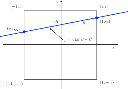
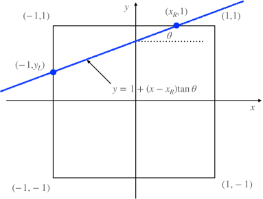
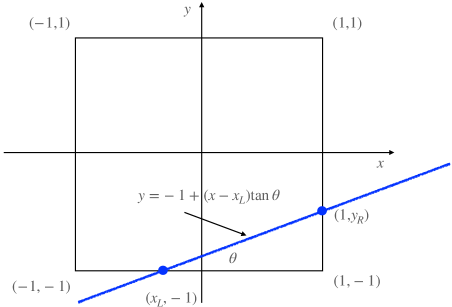
Figure 2. The sketch on the upper left shows the configuration in which the waterline (blue) intersects opposite sides of the square. The sketch on the upper right shows the configuration in which the waterline intersects adjacent sides of the square for $R>1/2$. The sketch on the bottom shows the configuration in which the waterline intersects adjacent sides of the square for $R<1/2$.

2.2.1. Waterline Intersects Opposite Sides of Square

Here we define the waterline by the equation

(2.8) $$y = x\tan\theta+H,$$

where $\theta$ is the slope of the waterline and $H$ is the y-intercept (see Figure 2). With the water assumed to occupy the region below the waterline, the submerged area can be written in terms of $H$ as $A_{\rm{sub}}=2(1+H)$. Therefore, Archimedes’ Principle requires $R=(1+H)/2$, or equivalently $H=2R-1$. Note that for $R\in(0,1)$ it follows that $H\in(-1,1)$.

We define waterline intersection points $(-1,y_{L})$ and $(1,y_{R})$ and note that

(2.9) $$y_{L}=-\tan\theta+H,\quad y_{R}=\tan\theta+H.$$

By definition, the configuration under consideration requires that $y_{L}\in[-1,1]$ and $y_{R}\in[-1,1]$. Furthermore, the largest and smallest $\theta$ occur for $y_{R}=\pm 1,y_{L}=\mp 1$, meaning that $-\pi/4\leq\theta\leq\pi/4$ and $-1\leq\tan\theta\leq 1.$ Combining these facts with the definitions of $y_{L}$ and $y_{R}$, we get

(2.10) $$\tan\theta+H\leq 1\hskip 18.06749pt\mbox{and}\hskip 18.06749pt-\tan\theta+H\leq 1\hskip 18.06749pt\mbox{if $H\geq 0$},$$

(2.11) $$-\tan\theta+H\geq-1\hskip 18.06749pt\mbox{and}\hskip 18.06749pt\tan\theta+H\geq-1\hskip 18.06749pt\mbox{if $H\leq 0$},$$

These can be rewritten as

(2.12) $$-1+|H|\leq\tan\theta\leq 1-|H|.$$

This range of $\tan\theta$ corresponds to a range of $\theta$ values $[\theta_{1}^{\min},\theta_{1}^{\max}]$ contained in $[-\pi/4,\pi/4]$. By symmetry, there is a corresponding configuration when rotated by $\pm\pi/2$ and $\pm\pi$.

The submerged area in this configuration is defined by the four points $(1,-1)$, $(1,y_{R})$, $(-1,y_{L})$, and $(-1,-1)$. We use (2.2) to find the center of buoyancy as the centroid of the submerged boundary region. In particular, let $(x_{k},y_{k})$ be given by $\{(1,-1),(1,y_{R}),(-1,y_{L}),(-1,-1),(1,-1)\}$. Then $\vec{B}(\theta)=(B_{x}(\theta),B_{y}(\theta))$ where

$$B_{x}(\theta) = \frac{1}{6A_{\rm{sub}}}\sum_{k=1}^{4}(x_{k}^{2}+x_{k}x_{k+1}+x_{k+1}^{2})(y_{k+1}-y_{k})$$

$$B_{y}(\theta) = \frac{1}{6A_{\rm{sub}}}\sum_{k=1}^{4}-(y_{k}^{2}+y_{k}y_{k+1}+y_{k+1}^{2})(x_{k+1}-x_{k})\;.$$

Computing these sums, combined with the values of $y_{L}$ and $y_{R}$ and the fact that $A_{\rm{sub}}=2(1+H)$, we find that the center of buoyancy takes the form

(2.13) $$\vec{B}(\theta)=\vec{B}_{1}(\theta) \equiv \frac{1}{2(1+H)}\Big{(}\frac{2}{3}\tan\theta,-1+H^{2}+\frac{1}{3}\tan^{2}\theta\Big{)},$$

where $\theta$ can take on any value defined by the inequalities (2.12). For use below we define this specific form for the center of buoyancy as $\vec{B}_{1}(\theta)$.

2.2.2. Waterline Intersects Adjacent Sides of Square

A similar approach can be applied to the second configuration shown in the upper right sketch of Figure 2. Here we give expressions for the results when $R\geq 1/2$ and when $R<1/2$.

Case 1: $R\geq 1/2$. Here we assume that the waterline intersects the left and top sides of the square at points $(-1,y_{L})$ and $(x_{R},1)$ so that three corners of the square are submerged. We consider the case $R<1/2$ in the next section although note that this case can be carefully extracted from the present case (according to Gilbert [Gilbert1991], Feigel & Fuzailov [FF2021], among others).

Here we identify the waterline by

(2.14) $$y = (x-x_{R})\tan\theta+1,$$

where $y_{L}=-(1+x_{R})\tan\theta+1$.

This waterline cuts a triangular region of area $\frac{1}{2}(1+x_{R})(1-y_{L})$ from the original square. This means that $A_{\rm{sub}}=4-\frac{1}{2}(1+x_{R})(1-y_{L})$ and

(2.15) $$R=\frac{A_{\rm{sub}}}{A_{\rm{obj}}} = \frac{4-\frac{1}{2}(1+x_{R})(1-y_{L})}{4}=\frac{4-\frac{1}{2}(1+x_{R})^{2}\tan\theta}{4}.$$

Rearranging this gives $x_{R}$ in terms of $R$ and the waterline slope $\tan\theta$

(2.16) $$(1+x_{R})^{2} = \frac{8-8R}{\tan\theta}.$$

Conditions on $\theta$ come from the requirement that $0\leq(1+x_{R})\leq 2$ and $-1\leq y_{L}\leq 1$. The first of these reveals that

(2.17) $$0\leq\frac{2-2R}{\tan\theta}\leq 1.$$

For the case under consideration $0<\theta<\frac{\pi}{2}$. It follows that $\tan\theta\geq 2-2R$. Equality corresponds to the waterline passing through the point $(1,1)$ and $(-1,y_{L})$. The other extreme corresponds to the waterline passing through the point $(-1,-1)$ and $(x_{R},1)$. This has $\tan\theta=2/(1+x_{R})$. Here the triangular area is $\frac{1}{2}2(1+x_{R})$ which means $R=(4-(1+x_{R}))/4$ or $(1+x_{R})=4-4R$. Since $\theta$ cannot exceed this angle we have $\tan\theta<2/(4-4R)$. Thus, for this configuration the value of $\tan\theta$ is constrained by

(2.18) $$2-2R\leq\tan\theta\leq\frac{1}{2-2R}.$$

As in the previous case, the center of buoyancy is obtained by calculating the centroid of the submerged area using (2.2). In particular, using the counterclockwise oriented vertices of the submerged polygon:

$$\{(x_{R},1),(-1,y_{L}),(-1,-1),(1,-1),(1,1)\},$$

we can calculate the following integral

(2.19) $$\vec{B}(\theta) = \frac{1}{A_{\rm{sub}}}\iint_{\Omega_{\rm sub}}(x,y)\;dA$$

as a sum. Evaluating this integral gives

(2.20) $$\vec{B}(\theta)=\vec{B}_{2}^{+}(\theta) \equiv \frac{1}{A_{\rm{sub}}}\Big{(}1-\frac{1}{2}(y_{L}+1)-\frac{1}{6}(x_{R}^{3}+1)\tan\theta,$$

$$\mbox{}-1+\frac{1}{2}(1-x_{R})+\frac{(1-y_{L}^{3})}{6\tan\theta}\Big{)}.$$

For use below, we define this specific form for the center of buoyancy as $\vec{B}_{2}^{+}(\theta)$. Recall that $A_{\rm{sub}}=4R$ and

(2.21) $$y_{L}=-\tan\theta(1+x_{R})+1,\quad(1+x_{R})^{2}=\frac{8-8R}{\tan\theta},$$

where $\tan\theta$ satisfies (2.18). This condition gives a range of $\theta$ values given by $[\theta_{2}^{+\min},\theta_{2}^{+\max}]$ contained in $[0,\pi/2]$. Again by symmetry, we get a corresponding set of angles by adding $\pm\pi/2,\pm\pi$.

Case 2: $R<1/2$. Here assume that the waterline intersects the square at points $(x_{L},-1)$ and $(1,y_{R})$ so that only the lower right corner of the square is submerged.

Here we identify the waterline by

(2.22) $$y = \tan\theta(x-x_{L})-1,$$

where $y_{R}=\tan\theta(1-x_{L})-1$.

This waterline cuts a triangular region of area $A_{sub}=\frac{1}{2}(1+y_{R})(1-x_{L})$ from the original square. This means that

(2.23) $$R=\frac{A_{\rm{sub}}}{A_{\rm{obj}}} = \frac{1}{8}(1+y_{R})(1-x_{L})=\frac{(1-x_{L})^{2}\tan\theta}{8}.$$

Rearranging this gives $x_{L}$ in terms of $R$ and the waterline slope $\tan\theta$

(2.24) $$(1-x_{L})^{2} = \frac{8R}{\tan\theta}.$$

Conditions on $\theta$ come from the requirement that $0\leq(1-x_{L})\leq 2$. This translates to

(2.25) $$\tan\theta\geq 2R.$$

Also the condition $-1\leq y_{R}\leq 1$ leads to

(2.26) $$0\leq\tan\theta\leq\frac{2}{1-x_{L}}.$$

Using $8R=(1-x_{L})(1+y_{R})$ leads to $0<\tan\theta<1/(2R)$.

So, together these require

(2.27) $$2R\leq\tan\theta\leq\frac{1}{2R}.$$

As before, the center of buoyancy satisfies

(2.28) $$\vec{B}(\theta) = \frac{1}{A_{\rm{sub}}}\int_{\Omega_{\rm sub}}(x,y)\;dA,$$

which can be calculated as a sum involving the vertices of the submerged polygonal cross section via  (2.2). It follows that

$$\vec{B}(\theta) = \vec{B}_{2}^{-}(\theta)$$

$$\equiv \frac{1}{A_{\rm{sub}}}\Big{(}\frac{y_{R}+1}{2}-\frac{(1-x_{L}^{3})}{6}\tan\theta,-\frac{(1-x_{L})}{2}+\frac{1+y_{R}^{3}}{6\tan\theta}\Big{)}\;.$$

For use below, we define this specific form for the center of buoyancy as $\vec{B}_{2}^{-}(\theta)$. Recall that $A_{\rm{sub}}=4R$ and

(2.30) $$y_{R}=\tan\theta(1-x_{L})-1,\quad(1-x_{L})^{2} = \frac{8R}{\tan\theta},$$

where $\tan\theta$ satisfies (2.27).

2.2.3. Potential Energy Expressions: Square Cross Section

As defined in  (2.6) the potential energy function is given by

$$U(\theta)=\hat{n}(\theta)\cdot(\vec{G}-\vec{B}(\theta)),$$

where the unit normal to the waterline can be expressed as a function of $\theta$ as $\hat{n}(\theta)=(-\sin\theta,\cos\theta)$. For the square defined above with uniform density the center of gravity $\vec{G}=(0,0)$. However, we are interested in a generalization of the square where the center of gravity, by some means, is not necessarily located at the center but rather has coordinates $\vec{G}=(G_{x},G_{y})$. Note that as long as Archimedes’ Principle is applied with the appropriate mass of the object, the calculations presented above for the center of buoyancy are independent of the location of the center of gravity. So, in what follows we treat $\vec{G}$ as nonzero in general.

For $R\geq 1/2$ define

(2.31) $$U_{B_{1}}(\theta) = \hat{n}(\theta)\cdot\vec{B}_{1}(\theta)\,,\mbox{ for }-1+|H|\leq\tan\theta\leq 1-|H|\,,$$

which corresponds to a range of $\theta\in[\theta_{1}^{\min},\theta_{1}^{\max}]$ defined by (2.12). Also define

(2.32) $$U_{B_{2}^{+}}(\theta) = \hat{n}(\theta)\cdot\vec{B}_{2}^{+}(\theta)\,,\mbox{ for }2-2R\leq\tan\theta\leq\frac{1}{2-2R}\,,$$

which corresponds to a range of $\theta\in[\theta_{2}^{+\min},\theta_{2}^{+\max}]$ defined by (2.18).

We can write the potential energy function $U(\theta)$ as follows

(2.40) $$U(\theta) = \left\{\begin{array}[]{ll}\hat{n}(\theta)\cdot\vec{G}-U_{B_{1}}(\theta)&\theta\in[\theta_{1}^{\min},\theta_{1}^{\max}]\\ \hat{n}(\theta)\cdot\vec{G}-U_{B_{1}}(\theta\pm\frac{\pi}{2})&\theta\pm\frac{\pi}{2}\in[\theta_{1}^{\min},\theta_{1}^{\max}]\\ \hat{n}(\theta)\cdot\vec{G}-U_{B_{1}}(\theta\pm\pi)&\theta\pm\pi\in[\theta_{1}^{\min},\theta_{1}^{\max}]\\ &\\ \hat{n}(\theta)\cdot\vec{G}-U_{B_{2}^{+}}(\theta)&\theta\in[\theta_{2}^{+\min},\theta_{2}^{+\max}]\\ \hat{n}(\theta)\cdot\vec{G}-U_{B_{2}^{+}}(\theta\pm\frac{\pi}{2})&\theta\pm\frac{\pi}{2}\in[\theta_{2}^{+\min},\theta_{2}^{+\max}]\\ \hat{n}(\theta)\cdot\vec{G}-U_{B_{2}^{+}}(\theta\pm\pi)&\theta\pm\pi\in[\theta_{2}^{+\min},\theta_{2}^{+\max}]\\ \end{array}\right.$$

A similar formula applies when $R<1/2$ (replace $B_{2}^{+}$ with $B_{2}^{-}$ and the corresponding range for $\tan\theta$ given in (2.27)).

2.3. Squares With Off-Center Weights

We also explore the case of a square cross section with an off-center weight parallel to the long axis of the object. Specifically we consider 3D printed objects with a hole in the square that can be filled with a material of different density. In our experiments we had the option to leave the hole as void space or to insert a nail cut to fit the object. In either case, before floating the object tape was placed over the holes to prevent water from filling the space.

For such a configuration we can predict the modified center of gravity $\vec{G}\neq 0$. In particular, consider the same square with corners at $(1,-1)$, $(1,1)$, $(-1,1)$, $(-1,-1)$ with a hole with circular cross section at point $(a,b)$ with $a\in(0,1)$, $b\in(0,1)$, and radius $r_{H}$. When such an object is printed there is a border around the hole whose thickness we denote by $t$ and whose density is $\rho_{\rm PLA}$ (i.e. the density of the solid print material). With the hole filled with a nail whose density is $\rho_{\rm nail}$ we can compute the center of gravity of the object as a whole (printed object plus nail) as

(2.41) $$M_{\rm{obj}}\vec{G} = L\left\{\int_{\Omega_{0}}\rho(\vec{x})\vec{x}\;dA+\int_{\Omega^{{\rm hole}+{\rm border}}}\rho(\vec{x})\vec{x}\;dA\right\},$$

where $M_{\rm{obj}}$ is the mass of the whole object (including the nail if one is inserted), $L$ is the length of the object, $\Omega_{0}$ denotes the cross-sectional domain of the square excluding the hole and border and $\Omega^{{\rm hole}+{\rm border}}$ denotes the circular cross section that includes the (printed) border of the hole and the hole, and $\rho(\vec{x})$ denotes the material density at position $\vec{x}$ in the plane. The square printed without a hole will have some void space in its interior and this can be controlled by changing the infill of the print. In our squares printed with a hole this infill region gets replaced by the hole plus the border material of the hole. Therefore, it is convenient to rewrite the formula (2.41) for center of gravity $\vec{G}$ as

(2.42) $$\frac{M_{\rm{obj}}}{L}\vec{G} = \int_{\Omega_{0}}\rho(\vec{x})\;\vec{x}\;dA+\int_{\Omega^{{\rm hole}+{\rm border}}}\rho(\vec{x})\;\vec{x}\;dA$$

$$\mbox{}+\int_{\Omega^{{\rm hole}+{\rm border}}}\rho_{\rm infill}\;\vec{x}\;dA-\int_{\Omega^{{\rm hole}+{\rm border}}}\rho_{\rm infill}\;\vec{x}\;dA,$$

$$= \int_{\Omega}\rho(\vec{x})\;\vec{x}\;dA+\int_{\Omega^{{\rm hole}+{\rm border}}}(\rho(\vec{x})-\rho_{\rm infill})\;\vec{x}\;dA,$$

where $\Omega$ denotes the cross section of the square undisturbed by a hole. Under our assumption of a square with uniform density the first integral in this expression equates to the zero vector. That is, for a square without the off-center hole the center of gravity is located at $(0,0)$. This requires that the infill is sufficiently symmetric about the center of the square so that it negligibly moves the center of gravity away from $(0,0)$. It follows that for the off-center square the center of gravity can then be estimated as

(2.43) $$\frac{M_{\rm{obj}}}{L}\vec{G} = \int_{\Omega^{{\rm hole}+{\rm border}}}(\rho(\vec{x})-\rho_{\rm infill})\;\vec{x}\;dA,$$

$$= (\rho_{\rm nail}-\rho_{\rm infill})\int_{0}^{2\pi}\int_{0}^{r_{H}}\vec{x}r\;dr\;d\theta$$

$$\mbox{}+(\rho_{\rm PLA}-\rho_{\rm infill})\int_{0}^{2\pi}\int_{r_{H}}^{r_{H}+t}\vec{x}r\;dr\;d\theta,$$

where each of the density terms in these expressions are assumed to be independent of position. These integrals can be evaluated writing $\vec{x}=(a+r\cos\theta,b+r\sin\theta)$. It follows that

(2.44) $$\frac{M_{\rm{obj}}}{L}\vec{G} = \pi(\rho_{\rm nail}-\rho_{\rm infill})r_{H}^{2}(a,b)+\pi(\rho_{\rm PLA}-\rho_{\rm infill})[(r_{H}+t)^{2}-r_{H}^{2}](a,b),$$

$$= \left\{\pi(\rho_{\rm nail}-\rho_{\rm infill})r_{H}^{2}+\pi(\rho_{\rm PLA}-\rho_{\rm infill})[2r_{H}t+t^{2}]\right\}(a,b).$$

So, for the off-center square with hole at $(a,b)$ the center of gravity is shifted towards $(a,b)$ from the origin by terms proportional to density differences and cross-sectional areas. Note that all of the quantities in this expression can be determined by straightforward measurements and are listed in Table 2.3.

Practically speaking, our prints are not completely uniform in the direction orthogonal to the square face since the top and bottom square faces are solid PLA. An improved estimate for the center of gravity that accounts for the two end faces of the square of thickness $t$ with density $\rho_{\rm PLA}$ is

(2.45) $$M_{\rm{obj}}\vec{G} = \Big{\{}\left[(\rho_{\rm nail}-\rho_{\rm infill})(\pi r_{H}^{2})+(\rho_{\rm PLA}-\rho_{\rm infill})\pi(2r_{H}t+t^{2})\right](L-2t)$$

$$\mbox{}+2t(\rho_{\rm nail}-\rho_{\rm PLA})(\pi r_{H}^{2})\Big{\}}(a,b),$$

$$= M_{\rm nail}(a,b)+\Big{\{}\left[-\rho_{\rm infill}(\pi r_{H}^{2})+(\rho_{\rm PLA}-\rho_{\rm infill})\pi(2r_{H}t+t^{2})\right](L-2t)$$

$$\mbox{}-2t\rho_{\rm PLA}(\pi r_{H}^{2})\Big{\}}(a,b).$$

That is, the new center of gravity, $\vec{G}$, is shifted towards the hole location $(a,b)$ by an amount related to the mass of the nail (we use $M_{\rm nail}=0$ for an open hole) and terms related to the thickness of the hole and the material it replaces (either infill or boundary).

Table 1. Various parameter values for 3D prints with square cross section and a hole. The values of $M_{\rm nail}$ and $\rho_{\rm nail}$ were obtained by noting that each nail was 60 mm in length and 2 mm in radius and that 25 nails weighed $137.51$ g.

$$\begin{array}{ccc}& & \\ \text{Parameter}& \text{Description}& \text{Value}\\ & & \\ I& \begin{array}{c}\text{Infill Fraction}\\ (\text{Infill \% /100})\end{array}& 0.05\mathrm{\dots }0.95\\ & & \\ s& \text{Length of Side of Square}& 30\text{mm}\\ & & \\ L& \text{Length of Object}& 60\text{mm}\\ & & \\ \rho {}_{\mathrm{PLA}}& \text{Density of PLA}& 1.15\text{ g cm}{}^{-3}\\ & & \\ M{}_{\mathrm{nail}}& \text{Mass of Nail}& 5.5004\text{ g}\\ & & \\ \rho {}_{\mathrm{nail}}& \begin{array}{c}\text{Density of Nail}\\ M{}_{\mathrm{nail}}/V{}_{\mathrm{nail}}\end{array}& 7.295\text{ g cm}{}^{-3}\\ & & \\ \rho {}_{\mathrm{infill}}& \begin{array}{c}\text{Effective Density of Infill}\\ \rho {}_{\mathrm{PLA}}\times I\end{array}& \text{varies with Infill}\\ & & \\ r{}_H& \text{Radius of Hole}& 2.5\text{mm}\\ & & \\ t& \text{Thickness of Solid Border}& 0.8\text{mm}\end{array}Thepredictedeffectivedensityfortheblockofsquarecrosssectionis\text{(2.46)2.46 , ρeffsquare=MsquareVext,}wherethetotalmassoftheobjectis\text{(2.47)2.47 - V)ρ + V I ρ, Msquare=(Vext - Vint)ρPLA + Vint I ρPLA,}and\text{V\_ext = s^2 L}and\text{V\_int = (s - 2t)^2 (L - 2t)}.Whentheblockisprintedwithaholeofradius\text{r\_H}paralleltothelongaxisthepredictedeffectivedensityis\text{(2.48)2.48 { M + M - πr [ 2 t + (L - 2t) I ] ρ +t) - r] (L - 2t) (ρ - I ρ) } ρeffsquare + hole=1Vext { Msquare + Mnail - πrH2 [ 2 t + (L - 2t) I ] ρPLA + π[ (rH +t)2 - rH2] (L - 2t) (ρPLA - I ρPLA) }}Theeffectivedensityoftheobjectwithoutthenailfillingtheholeiscalculatedbythesameformulawith\text{M\_nail}settozero.Variouscomparisonsbetweenthistheoryandourexperimentalobservationsandmeasurementsaregivenbelow.First,however,weneedtocreateourfloatingobjects.\text{33§33Methodsfor3DPrinting3Meth}$$