Study of Robust Sparsity-Aware RLS algorithms with Jointly-Optimized Parameters for Impulsive Noise Environments

Abstract

This paper proposes a unified sparsity-aware robust recursive least-squares RLS (S-RRLS) algorithm for the identification of sparse systems under impulsive noise. The proposed algorithm generalizes multiple algorithms only by replacing the specified criterion of robustness and sparsity-aware penalty. Furthermore, by jointly optimizing the forgetting factor and the sparsity penalty parameter, we develop the jointly-optimized S-RRLS (JO-S-RRLS) algorithm, which not only exhibits low misadjustment but also can track well sudden changes of a sparse system. Simulations in impulsive noise scenarios demonstrate that the proposed S-RRLS and JO-S-RRLS algorithms outperform existing techniques.

I Introduction

In realistic environments, in addition to Gaussian noise, impulsive noise is often present such as in echo cancellation, underwater acoustics, audio processing, and communications [1, 2, 3]. Realizations of the impulsive noise are random and sparse in the time domain, and typically have much higher amplitudes than Gaussian noise. In these scenarios, the popular recursive least squares (RLS) algorithm experiences significant performance deterioration.

Aiming at impulsive noise cases, various strategies have been applied to develop robust adaptive algorithms [4, 5, 6, 7, 8, 9, 10], [11, 12, 13, 14, 15, 16, 17, 18, 19, 20, 21, 22, 23, 24, 25, 26, 27, 28, 29, 30, 31, 32, 33, 34, 35, 36, 37, 38, 39, 40, 41, 42, 43, 44, 45, 46, 47, 48, 49, 50, 51, 52, 53, 54, 55, 56, 57, 58, 59, 60, 61, 62, 63, 64, 65, 66, 67, 68, 69, 70, 71, 72, 73, 74, 75, 76, 77, 78, 79, 80, 81, 82, 83], In particular, the recursive least M-estimate (RLM) algorithm was proposed by introducing the M-estimator of the error signal [4]; it not only shows good robustness against impulsive noises, but also almost retains the fast convergence which the RLS algorithm possesses in the Gaussian noise. The correntropy defines similarity between two variables so that it has the property to identify normal and abnormal samples [10]. Based on this property, the recursive maximum correntropy criterion (RMCC) algorithm was presented [9], which is capable of dealing with impulsive noises.

In studying adaptive algorithms, there is interest to exploit the system sparsity. A sparse vector signifies that it only has a few non-zero entries such as the impulse responses of propagation channels in underwater acoustic and terrestrial communications [84, 85, 86]. With different sparsity-aware penalties (e.g., the $l_{1}$-norm, $l_{0}$-norm, and logarithmic based penalties), several sparsity-aware variants of the standard RLS algorithm were reported [87, 88], which reduce the steady-state misadjustment. Likewise, in the impulsive noise environment, sparsity-aware robust RLS-type algorithms were proposed, such as the sparsity-aware RLM algorithm [89] and the sparsity-aware RMCC algorithm [90]. However, it is worth noting that these algorithms have two drawbacks. First, they use the constant forgetting factor that controls the trade-off between the steady-state misadjustment and tracking capability for sudden changes of systems. Second, their performance depends on the sparsity-penalty parameter, which is usually chosen in a trial-and-error way, thus limiting their usefulness. In the literature, these two problems were separately considered for Gaussian noise scenarios. As such, variable forgetting factor (VFF) [91, 92, 93] and variable sparsity-penalty parameter (VSPP) [87] schemes have been developed. Nevertheless, they have not been considered jointly and for impulsive noise scenarios.

In this paper, our contributions are as follows. 1) We propose a unified S-RRLS framework, which covers different algorithms by applying straightforwardly the specified robustness criterion and sparsity-aware penalty. 2) By decoupling the effect of forgetting factor and sparsity-penalty parameter from each other, we derive adaptive rules for adjusting online these two parameters, and therefore the resulting jointly-optimized S-RRLS (JO-S-RRLS) algorithm reaches a low steady-state misadjustment and good tracking capability in impulsive noise.

The remaining part of this paper is organized as follows. Section II reviews the signal model and introduces the S-RRLS framework. In Section III, we present the JO-S-RRLS algorithm. Section IV shows simulations results. Conclusions are presented in Section V.

II Signal Model and S-RRLS Algorithm

Consider a system identification problem with the input signal $x_{k}$ at time $k$, then the output $d_{k}$ of the system is described by

$$d_{k}=\bm{x}_{k}^{\text{T}}\bm{w}^{o}+v_{k},$$ (1)

where $\bm{w}^{o}\in\mathbb{R}^{M\times 1}$ is the impulse response of the sparse system to be identified, $\bm{x}_{k}=[x_{k},x_{k-1},...,x_{k-M+1}]^{\text{T}}\in\mathbb{R}^{M\times 1}$ is the input vector, and $v_{k}$ is the noise. An estimate of $\bm{w}^{o}$ at time $k$, the vector of coefficients of adaptive filter, is denoted by $\bm{w}_{k}\in\mathbb{R}^{M\times 1}$. For updating the filter coefficients in Gaussian noise, the sparsity-aware RLS algorithm that exploits the sparsity of $\bm{w}^{o}$ is popular. However, the surroundings noise may also include impulsive samples which deteriorate the algorithm performance. For such scenarios, we introduce the unified robust sparsity-aware minimization problem:

$$\bm{w}_{k}=\arg\min\limits_{\bm{w}_{k}}\left\{\sum\limits_{j=0}^{k}\lambda^{k-j}\varphi\left(d_{j}-\bm{x}_{j}^{\text{T}}\bm{w}_{k}\right)+\rho f(\bm{w}_{k})\right\},$$ (2)

where $0<\lambda<1$ is the forgetting factor and $\varphi(\cdot):\mathbb{R}\rightarrow\mathbb{R}$ is a robustness function that can deal with impulsive noise. In (2), $f(\cdot):\mathbb{R}^{M\times 1}\rightarrow\mathbb{R}$ is a general sparsity-aware penalty function, and $\rho>0$ is the sparsity-aware penalty parameter defining the weight of this penalty term. By solving the optimization in (2), we obtain the following normal equation:

$$\bm{R}_{k}\bm{w}_{k}=\bm{z}_{k}-\rho\triangledown f(\bm{w}_{k}),$$ (3)

where

$$\begin{array}[]{rcl}\begin{aligned} \bm{R}_{k}=\sum\limits_{j=0}^{k}\lambda^{k-j}q_{j}\bm{x}_{j}\bm{x}_{j}^{\text{T}}=\lambda\bm{R}_{k-1}+q_{k}\bm{x}_{k}\bm{x}_{k}^{\text{T}}\\ \bm{z}_{k}=\sum\limits_{j=0}^{k}\lambda^{k-j}q_{j}d_{j}\bm{x}_{j}=\lambda\bm{z}_{k-1}+q_{k}d_{n}\bm{x}_{k}\end{aligned}\end{array}$$ (4)

are the time-averaged autocorrelation matrix of $\bm{x}_{k}$ and the time-averaged crosscorrelation vector of $d_{k}$ and $\bm{x}_{k}$, respectively, and $\triangledown f(\bm{w}_{k})$ is the subgradient of $f(\bm{w}_{k})$ with respect to $\bm{w}_{k}$. Also, $q_{k}=\varphi^{\prime}(\epsilon_{k})/\epsilon_{k}$, where $\epsilon_{k}=d_{k}-\bm{x}_{k}^{\text{T}}\bm{w}_{k}$ is the a posteriori error and $\varphi^{\prime}(\epsilon_{k})$ is the derivative of $\varphi(\epsilon_{k})$.

Applying the matrix inversion lemma [94], we have

$$\begin{array}[]{rcl}\begin{aligned} \bm{P}_{k}\triangleq\bm{R}_{k}^{-1}=\frac{1}{\lambda}\left(\bm{P}_{k-1}-\bm{K}_{k}\bm{x}_{k}^{T}\bm{P}_{k-1}\right),\end{aligned}\end{array}$$ (5)

where

$$\begin{array}[]{rcl}\begin{aligned} \bm{K}_{k}\triangleq\frac{q_{k}\bm{P}_{k-1}\bm{x}_{k}}{\lambda+q_{k}\bm{x}_{k}^{T}\bm{P}_{k-1}\bm{x}_{k}}\end{aligned}\end{array}$$ (6)

is the Kalman gain vector, and $\bm{P}_{k}$ is initialized by $\bm{P}_{0}=\delta^{-1}\bm{I}_{M}$ with $\delta>0$ being the regularization parameter. Then, substituting (5) and (6) into (3), the recursion for $\bm{w}_{k}$ is established:

$$\begin{array}[]{rcl}\begin{aligned} \bm{w}_{k}=\bm{w}_{k-1}+\bm{K}_{k}e_{k}-\rho\bm{P}_{k}[\triangledown f(\bm{w}_{k})-\lambda\triangledown f(\bm{w}_{k-1})],\end{aligned}\end{array}$$ (7)

where $e_{k}=d_{k}-\bm{x}_{k}^{\text{T}}\bm{w}_{k-1}$ is the a priori error. Naturally, the above recursion is not realizable, since $q_{k}$ and $\triangledown f(\bm{w}_{k})$ require knowing $\bm{w}_{k}$ at time $k$ beforehand. To overcome this problem, it is assumed that $q_{k}$ and $\triangledown f(\bm{w}_{k})$ do not change considerably at adjacent time. Hence, we can rewrite (7) as

$$\begin{array}[]{rcl}\begin{aligned} \bm{w}_{k}=\bm{w}_{k-1}+\bm{K}_{k}e_{k}-\rho\bm{P}_{k}\triangledown f(\bm{w}_{k-1}),\end{aligned}\end{array}$$ (8)

where $(1-\lambda)$ is absorbed into $\rho$ that is $\rho\leftarrow\rho(1-\lambda)$, and we can approximate $q_{k}$ as

$$q_{k}\approx\varphi^{\prime}(e_{k})/e_{k}.$$ (9)

III Proposed JO-S-RRLS Algorithm

Clearly, the S-RRLS algorithm performance depends on the parameters $\lambda$ and $\rho$. Specifically, $\lambda$ governs the trade-off between steady-state error and tracking capability through the Kalman gain vector. The parameter $\rho$ must be properly chosen to ensure that the S-RRLS algorithm fully exploits the system’s sparsity and thus outperforms the RRLS algorithm. In this section, we design adaptive schemes for $\lambda$ and $\rho$, producing time-varying parameters $\lambda_{k}$ and $\rho_{k}$. For this purpose, we rearrange (8) in two steps as

$$\bm{\psi}_{k} =\bm{w}_{k-1}+\bm{K}_{k}e_{k},$$ (10a)

$$\bm{w}_{k} =\bm{\psi}_{k}-\rho_{k}\bm{P}_{k}\triangledown f(\bm{\psi}_{k}).$$ (10b)

The step (10a) plays the adaptive learning role of the RRLS algorithm; the step (10b) drives inactive coefficients in $\bm{\psi}_{k}$ to zero, thereby improving the performance of identifying sparse $\bm{w}^{o}$. Importantly, we also replace the original $\triangledown f(\bm{w}_{k-1})$ in (10b) with $\triangledown f(\bm{\psi}_{k})$. In doing so, $\lambda_{k}$ and $\rho_{k}$ will be designed independently according to (10a) and (10b), respectively.

III-A Design of $\rho_{k}$

By subtracting (10b) from $\bm{w}^{o}$, we obtain

$$\begin{array}[]{rcl}\begin{aligned} \widetilde{\bm{w}}_{k}=\widetilde{\bm{\psi}}_{k}+\rho_{k}\bm{P}_{k}\triangledown f(\bm{\psi}_{k}),\end{aligned}\end{array}$$ (11)

where $\widetilde{\bm{w}}_{k}\triangleq\bm{w}^{o}-\bm{w}_{k}$ and $\widetilde{\bm{\psi}}_{k}\triangleq\bm{w}^{o}-\bm{\psi}_{k}$ represent the deviation vectors for the estimates $\bm{w}_{k}$ and $\bm{\psi}_{k}$. Taking the $l_{2}$-norm on both sides of (11), it is found that

$$\begin{array}[]{rcl}\begin{aligned} ||\widetilde{\bm{w}}_{k}&||_{2}^{2}=||\widetilde{\bm{\psi}}_{k}||_{2}^{2}+\\ &\underbrace{2\rho_{k}\widetilde{\bm{\psi}}_{k}^{T}\left(\bm{P}_{k}\triangledown f(\bm{\psi}_{k})\right)+\rho_{k}^{2}||\bm{P}_{k}\triangledown f(\bm{\psi}_{k})||_{2}^{2}}_{\bigtriangleup_{k}}.\end{aligned}\end{array}$$ (12)

Minimizing $||\widetilde{\bm{w}}_{k}||_{2}^{2}$ with respect to $\rho_{k}$, the optimal $\rho_{k}$ is obtained as

$$\begin{array}[]{rcl}\begin{aligned} \rho_{k}^{\text{opt}}=\frac{[\bm{\psi}_{k}-\bm{w}^{o}]^{T}\left(\bm{P}_{k}\triangledown f(\bm{\psi}_{k})\right)}{||\bm{P}_{k}\triangledown f(\bm{\psi}_{k})||_{2}^{2}}.\end{aligned}\end{array}$$ (13)

At time $k$, although we do not know the true $\bm{w}^{o}$ in (13), it can be approximated by the previous estimate $\bm{w}_{k-1}$ from (10b). Thus, we modify (13) to the following rule for choosing $\rho_{k}$:

$$\begin{array}[]{rcl}\begin{aligned} \hat{\rho}_{k}^{\text{opt}}=\max\left[\frac{[\bm{\psi}_{k}-\bm{w}_{k-1}]^{T}\left(\bm{P}_{k}\triangledown f(\bm{\psi}_{k})\right)}{||\bm{P}_{k}\triangledown f(\bm{\psi}_{k})||_{2}^{2}},\;0\right].\end{aligned}\end{array}$$ (14)

Also, since the estimate $\bm{w}_{k}$ at the early stage of the adaptation has a larger deviation as compared to $\bm{w}^{o}$, we enforce $\hat{\rho}_{k}^{\text{opt}}=0$ when $k\leq M/2$, to ensure the algorithm’s convergence.

III-B Design of $\lambda_{k}$

To derive the VFF scheme, we insert (6) into (10a) to yield

$$\begin{array}[]{rcl}\begin{aligned} \bm{\psi}_{k}&=\bm{w}_{k-1}+\frac{q_{k}\bm{P}_{k-1}\bm{x}_{k}}{\lambda_{k}+\theta_{k}}e_{k},\end{aligned}\end{array}$$ (15)

where $\theta_{k}=q_{k}\bm{x}_{k}^{T}\bm{P}_{k-1}\bm{x}_{k}$. By defining the intermediate error $\xi_{k}=d_{k}-\bm{x}_{k}^{\text{T}}\bm{\psi}_{k}$, we can find from (15) that

$$\begin{array}[]{rcl}\begin{aligned} \xi_{k}=\left(1-\frac{\theta_{k}}{\lambda_{k}+\theta_{k}}\right)e_{k}.\end{aligned}\end{array}$$ (16)

Inspired by [91], we propose to impose the condition

$$\begin{array}[]{rcl}\begin{aligned} E\{\xi_{k}^{2}\}=\sigma_{v}^{2}\end{aligned}\end{array}$$ (17)

on (16), which helps to recover the system noise in the intermediate error signal, where $E\{\cdot\}$ denotes the mathematical expectation. However, it is emphasized that $\sigma_{v}^{2}$ in (17) denotes the variance of the noise excluding impulsive noise samples, due to the fact that the negative influence of impulsive noises can be transferred to $q_{k}$ given in (9) (see the following subsection C for more explanation). For solving (17), we introduce two assumptions: 1) the a priori error and input signals are uncorrelated, i.e., the orthogonality principle [94]; 2) the forgetting factor is deterministic at each time [91, 93]. As a result, the solution of (17) with respect to $\lambda_{k}$ is given as

$$\begin{array}[]{rcl}\begin{aligned} \lambda_{k}=\frac{\sigma_{\theta,k}\sigma_{v}}{\sigma_{e,k}-\sigma_{v}},\end{aligned}\end{array}$$ (18)

where $\sigma_{e,k}^{2}=E\{e_{k}^{2}\}$ and $\sigma_{\theta,k}^{2}=E\{\theta_{k}^{2}\}$ are the variances of the corresponding signals. Both $\sigma_{e,k}^{2}$ and $\sigma_{\theta,k}^{2}$ could be estimated in a recursive way:

$$\hat{\sigma}_{e,k}^{2} =\chi\hat{\sigma}_{e,k-1}^{2}+(1-\chi)q_{k}^{2}e_{k}^{2},$$ (19a)

$$\hat{\sigma}_{\theta,k}^{2} =\chi\hat{\sigma}_{\theta,k-1}^{2}+(1-\chi)\theta_{k}^{2},$$ (19b)

where $q_{k}^{2}$ aims to reduce the negative influence of the impulsive noise on the estimated variance $\hat{\sigma}_{e,k}^{2}$ and $\chi\in[0.9,1)$ is a the smoothing factor. To estimate the variance $\sigma_{v}^{2}$ of the background noise, we extend the approach in [93] to impulsive noise environments, formulated as

$$\begin{array}[]{rcl}\begin{aligned} \hat{\sigma}_{v,k}^{2}=\frac{\hat{\sigma}_{d,k}^{2}\hat{\sigma}_{e,k}^{2}}{\hat{\sigma}_{e,k}^{2}+\hat{\sigma}_{y,k}^{2}},\end{aligned}\end{array}$$ (20)

where the estimated powers $\hat{\sigma}_{d,k}^{2}$ and $\hat{\sigma}_{y,k}^{2}$ are calculated similar to (19a) as

$$\hat{\sigma}_{d,k}^{2} =\chi\hat{\sigma}_{d,k-1}^{2}+(1-\chi)q_{k}^{2}d_{k}^{2},$$ (21a)

$$\hat{\sigma}_{y,k}^{2} =\chi\hat{\sigma}_{y,k-1}^{2}+(1-\chi)y_{k}^{2},$$ (21b)

with $y_{k}=\bm{x}_{k}^{\text{T}}\bm{w}_{k-1}$ being the output of the adaptive filter. Due to using the power estimates, it could happen that $\hat{\sigma}_{e,k}^{2}<\hat{\sigma}_{v,k}^{2}$; however, (18) shows that this situation has to be prevented. As such, we could set $\lambda_{k}$ to $\lambda_{\max}$ which is close to one. Furthermore, in the steady-state $\hat{\sigma}_{e,k}^{2}$ may vary around $\hat{\sigma}_{v,k}^{2}$. Therefore, we propose a more practical solution for $\lambda_{k}$ by imposing the convergence state $\hat{\sigma}_{e,k}^{2}<\tau\hat{\sigma}_{v,k}^{2}$ with $\tau\in[1,2]$, as follows:

$$\lambda_{k}=\left\{\begin{aligned} &\lambda_{\max},\;\text{if }\hat{\sigma}_{e,k}^{2}<\tau\hat{\sigma}_{v,k}^{2},\\ &\min\left\{\frac{\hat{\sigma}_{\theta,k}\hat{\sigma}_{v}}{|\hat{\sigma}_{e,k}-\hat{\sigma}_{v}|+\kappa},\lambda_{\max}\right\},\;\text{otherwise},\end{aligned}\right.$$ (22)

where $\kappa$ is a small positive constant. This completes the VFF’s derivation for the S-RRLS algorithm.

By equipping S-RRLS with the proposed $\hat{\rho}_{k}^{\text{opt}}$ and $\lambda_{k}$ adaptations, we arrive at the JO-S-RRLS algorithm. In fact, the proposed $\hat{\rho}_{k}^{\text{opt}}$ and $\lambda_{k}$ originate from the alternating optimization idea which is a powerful way to solve the challenging global optimization problems [95, 96].

Remark 1: As can be seen in (12), the term $\bigtriangleup_{k}$ results from the sparsity-aware step (10b). Only when $\bigtriangleup_{k}<0$, the S-RRLS algorithm will work better than the RRLS algorithm. Accordingly, $\rho$ must satisfy the inequality $0<\rho<2\rho_{k}^{\text{opt}}$. Following a similar derivation in Appendix D in [97], $\bigtriangleup_{k}<0$ is likely to be true when identifying a sparse vector $\bm{w}^{o}$. It follows that the optimal $\rho_{k}^{\text{opt}}$ given in (14) may exist. In the future, we will analyze the mean and mean-square behaviors of the JO-S-RRLS algorithm.

III-C Practical considerations

For implementing the S-RRLS and JO-S-RRLS algorithms, two problems should be addressed.

Firstly, the robustness of the algorithms against impulsive noises relies on how to design the robustness function $\varphi(e_{k})$ to further obtain $q_{k}$ in (9). As an example, the modified M-estimator is used [4], i.e., $\varphi(e_{k})=\left\{\begin{aligned} &e_{k}^{2}/2,\text{ if }|e_{k}|\leq\xi,\\ &\xi^{2}/2,\text{ if }|e_{k}|>\xi,\end{aligned}\right.$ such that $q_{k}=\left\{\begin{aligned} &1,\text{ if }|e_{k}|\leq\xi,\\ &0,\text{ if }|e_{k}|>\xi,\end{aligned}\right.$. It reveals that when $|e_{k}|>\xi$ holds (generally, when the impulsive noise happens), the Kalman gain $\bm{K}_{k}$ will be a zero vector due to $q_{k}=0$, thus stopping the update of the adaptive filter. The threshold $\xi$ is chosen as $\xi=\vartheta\hat{\sigma}_{\varepsilon,k}$,  $\hat{\sigma}_{\varepsilon,k}^{2}=\zeta\hat{\sigma}_{\varepsilon,k-1}^{2}+c_{\sigma}(1-\zeta)\text{med}(\bm{a}_{k}^{\varepsilon})$, where $\zeta\in[0.9,1)$ is an exponentially weighting factor (except $\zeta=0$ at time $k=0$), the median operator $\text{med}(\cdot)$ is to remove data in the window $\bm{a}_{k}^{\varepsilon}=[e_{k}^{2},e_{k-1}^{2},...,e_{k-N_{w}+1}^{2}]$ disturbed by impulsive noises, and $c_{\sigma}=1.483(1+5/(N_{w}-1))$ is the correction factor. Note that the window length $N_{w}$ needs to be properly chosen. Larger $N_{w}$ provide a more robust estimate $\hat{\varepsilon}_{e,k}^{2}$ but require a higher complexity [4]. Also, the value of $\vartheta$ is often chosen as 2.576 [4].

Secondly, to effectively characterize the sparsity of systems, how to design $f(\cdot)$ in (2) is also a key factor. Here we choose the popular log-penalty $f(\bm{w}_{k})=\sum_{m=1}^{M}\ln(1+|w_{m,k}|/\mu)$ [97], where $w_{m,k}$ denotes the $m$-th entry of $\bm{w}_{k}$, and $\mu>0$ denotes the shrinkage factor that helps to distinguish non-zero and zero entries. Thus, the entries of $\triangledown(\bm{\psi}_{m,k})$ in (10b) are given by $\triangledown(\psi_{m,k})=\frac{\text{sgn}(\psi_{m,k})}{\mu+|\psi_{m,k}|},m=1,...,M$.

It needs to point out that other robust criteria  [5, 6, 7, 8, 9, 98] and sparsity-aware penalties [87, 86, 97, 96] can also be applied to present different JO-S-RRLS algorithms. However, discussing the effects of different choices of $\varphi(e_{k})$ or $f(\bm{w}_{k})$ is not the focus of this paper.

Remark 2: Compared with the original S-RRLS algorithm, the extra computational complexity of the JO-S-RRLS algorithm stems from the adaptations of $\rho_{k}$ and $\lambda_{k}$, which requires $M^{2}+3M+13$ multiplications, $M^{2}+2M+6$ additions, $3$ divisions, and $3$ square-roots per iteration.

IV Simulation Results

In this section, simulations are presented to evaluate the proposed JO-S-RRLS algorithm. It is assumed that the length of the adaptive filter is the same as that of the unknown sparse vector $\bm{w}^{o}$. The input signal $x_{k}$ is generated by filtering a zero-mean white Gaussian random process $\nu_{k}$ with unit variance through a second-order autoregressive model $x_{k}=0.4x_{k-1}-0.4x_{k-2}+\nu_{k}$. The normalized mean square deviation is used as the performance measure, defined as $\text{NMSD}_{k}=10\log_{10}(||\bm{w}_{k}-\bm{w}^{o}||_{2}^{2}/||\bm{w}^{o}||_{2}^{2})$. All the curves are obtained by averaging the results over 100 independent runs.

Case 1: The sparse vector $\bm{w}^{o}$ has $M=64$ elements, and its non-zero elements follow from a zero-mean Gaussian distribution with variance $1/\sqrt{Q}$ and their positions are randomly selected from the binomial distribution, with $Q$ being the number of non-zero elements. A smaller $Q$ means sparser $\bm{w}^{o}$. The vector $\bm{w}^{o}$ cardinality changes from $Q=4$ to $Q=8$ at time $k=1501$. The noise with impulsive behavior $v_{k}$ is drawn from the contaminated-Gaussian (CG) process, i.e., $v_{k}=v_{k}^{\text{g}}+v_{k}^{\text{i}}$. Specifically, $v_{k}^{\text{g}}$ is zero-mean white Gaussian noise, with variance $\sigma_{\text{g}}^{2}$ given by the signal-to-noise ratio of 30 dB. The impulsive noise $v_{k}^{\text{i}}$ is described as $v_{k}^{\text{i}}=b_{k}\eta_{k}$, where $b_{k}$ follows from the Bernoulli distribution with the probabilities $P\{b_{k}=1\}=p$ and $P\{b_{k}=0\}=1-p$, and $\eta_{k}$ is also zero-mean white Gaussian noise with a large variance of $\sigma_{\eta}^{2}=1000E\{(\bm{x}_{k}^{\text{T}}\bm{w}^{o})^{2}\}$. Fig. 1 compares the proposed S-RRLS and JO-S-RRLS algorithms with the existing RLS, S-RLS, and RLM algorithms. To fairly evaluate them, we set $\lambda=0.995$ and $\delta=0.5$ for all the algorithms, the M-estimate parameter $N_{w}=9$ and $\zeta=0.99$ for all the robust algorithms, the log-penalty parameter $\mu=0.01$ for all the sparsity-aware algorithms. As expected, the RLS and S-RLS algorithms are not suitable for impulsive noise scenarios due to the performance degradation, while other algorithms show good robustness. Benefited from the sparsity-aware step, S-RRLS algorithm reduces the steady-state misadjustment in sparse systems as compared to the RLM algorithm. Also, by using the proposed adaptation of $\rho$, the S-RRLS algorithm with $\rho_{k}^{\text{opt}}$ avoids the choice problem of $\rho$. To deal with the sudden change of $\bm{w}^{o}$, we may also resort to the reset (Rs) technique, namely, the S-RRLS with $\rho_{k}^{\text{opt}}$ and Rs algorithm recovers the tracking capability. Importantly, by jointly optimizing $\rho$ and $\lambda$, the proposed JO-S-RRLS algorithm not only obtains a low steady-state misadjustment but also good tracking capability.

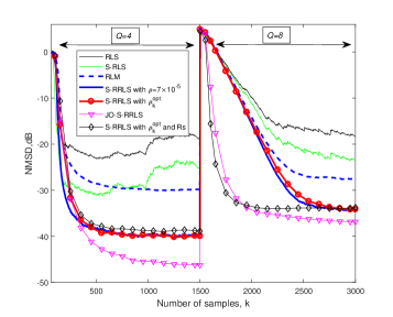
Figure 1: NMSD performance of RLS-type algorithms in the CG noise with $p=0.001$. The VFF’s parameters are set to $\lambda_{\max}=0.99999,\chi=0.96$, and $\tau=1.5$.

Case 2: The sparse vector $\bm{w}^{o}$ is the echo channel 1 from the ITUT G.168 standard, with $M=256$ taps [100]. The noise with impulsive behavior $v_{k}$ follows from the symmetric $\alpha$-stable random process, called the $\alpha$-stable noise. Its characteristic function [1] is given as $\phi(t)=\exp(-\gamma\lvert t\lvert^{\alpha})$, where $\alpha\in(0,2]$ describes the impulsiveness of the noise (smaller $\alpha$ corresponds to stronger impulsive noises) and $\gamma>0$ is similar to the variance of the noise. Note that when $\alpha=2$, it reduces to the Gaussian distribution. In Fig 2, we set $\alpha=1.65$ and $\gamma=0.02$. As one can see, the proposed JO-S-RRLS algorithm achieves the best performance among these algorithms, since it optimizes the parameters $\rho$ and $\lambda$ simultaneously.

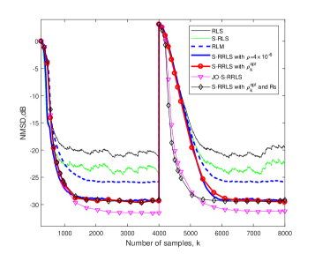
Figure 2: NMSD performance of RLS-type algorithms in the $\alpha$-stable noise. Some parameters are retuned as: $\lambda=0.977$, $N_{w}=16$, and $\mu=0.001$ for all the algorithms.

V Conclusion

In this work, a unified S-RRLS algorithm update was presented, which aims at identifying sparse systems in impulsive noise. By replacing straightforwardly the specified robustness criterion and sparsity-aware penalty, it can lead to different S-RRLS algorithms. We then developed adaptive schemes for both the forgetting factor and the sparsity penalty parameter in the S-RRLS algorithm, thus arriving at the JO-S-RRLS algorithm with a further improved performance in terms of the steady-state misadjustment and tracking capability. Simulations in various impulsive noise scenarios have been conducted to verify the effectiveness of the proposed algorithms.

References

- [1] C. L. Nikias and M. Shao, Signal processing with Alpha-stable distributions and applications. Wiley-Interscience, 1995.
- [2] M. Zimmermann and K. Dostert, “Analysis and modeling of impulsive noise in broad-band powerline communications,” IEEE Transactions on Electromagnetic Compatibility, vol. 44, no. 1, pp. 249–258, 2002.
- [3] Y. Yu, L. Lu, Z. Zheng, W. Wang, Y. Zakharov, and R. C. de Lamare, “DCD-based recursive adaptive algorithms robust against impulsive noise,” IEEE Transactions on Circuits and Systems II: Express Briefs, vol. 67, no. 7, pp. 1359–1363, 2020.
- [4] S.-C. Chan and Y.-X. Zou, “A recursive least M-estimate algorithm for robust adaptive filtering in impulsive noise: fast algorithm and convergence performance analysis,” IEEE Transactions on Signal Processing, vol. 52, no. 4, pp. 975–991, 2004.
- [5] Á. Navia-Vazquez and J. Arenas-Garcia, “Combination of recursive least -norm algorithms for robust adaptive filtering in alpha-stable noise,” IEEE Transactions on Signal Processing, vol. 60, no. 3, pp. 1478–1482, 2012.
- [6] H. Zayyani, “Continuous mixed -norm adaptive algorithm for system identification,” IEEE Signal Processing Letters, vol. 21, no. 9, pp. 1108–1110, 2014.
- [7] L. Lu, W. Wang, X. Yang, W. Wu, and G. Zhu, “Recursive Geman-Mcclure estimator for implementing second-order Volterra filter,” IEEE Transactions on Circuits and Systems II: Express Briefs, vol. 66, no. 7, pp. 1272–1276, 2019.
- [8] L. Lu, H. Zhao, and B. Chen, “Improved-variable-forgetting-factor recursive algorithm based on the logarithmic cost for Volterra system identification,” IEEE Transactions on Circuits and Systems II: Express Briefs, vol. 63, no. 6, pp. 588–592, 2016.
- [9] H. Radmanesh and M. Hajiabadi, “Recursive maximum correntropy learning algorithm with adaptive kernel size,” IEEE Transactions on Circuits and Systems II: Express Briefs, vol. 65, no. 7, pp. 958–962, 2018.
- [10] B. Chen, L. Xing, H. Zhao, N. Zheng, and J. C. Príncipe, “Generalized correntropy for robust adaptive filtering,” IEEE Transactions on Signal Processing, vol. 64, no. 13, pp. 3376–3387, 2016.
- [11] R. C. de Lamare and R. Sampaio-Neto, “Adaptive reduced-rank processing based on joint and iterative interpolation, decimation, and filtering,” IEEE Transactions on Signal Processing, vol. 57, no. 7, pp. 2503–2514, 2009.
- [12] R. C. de Lamare and R. Sampaio-Neto, “Minimum mean-squared error iterative successive parallel arbitrated decision feedback detectors for ds-cdma systems,” IEEE Transactions on Communications, vol. 56, no. 5, pp. 778–789, 2008.
- [13] R. de Lamare and R. Sampaio-Neto, “Adaptive reduced-rank mmse filtering with interpolated fir filters and adaptive interpolators,” IEEE Signal Processing Letters, vol. 12, no. 3, pp. 177–180, 2005.
- [14] R. C. de Lamare, “Adaptive and iterative multi-branch mmse decision feedback detection algorithms for multi-antenna systems,” IEEE Transactions on Wireless Communications, vol. 12, no. 10, pp. 5294–5308, 2013.
- [15] R. C. de Lamare and R. Sampaio-Neto, “Reduced-rank adaptive filtering based on joint iterative optimization of adaptive filters,” IEEE Signal Processing Letters, vol. 14, no. 12, pp. 980–983, 2007.
- [16] R. C. de Lamare and R. Sampaio-Neto, “Reduced-rank space-time adaptive interference suppression with joint iterative least squares algorithms for spread-spectrum systems,” IEEE Transactions on Vehicular Technology, vol. 59, no. 3, pp. 1217–1228, 2010.
- [17] R. C. de Lamare and R. Sampaio-Neto, “Adaptive reduced-rank equalization algorithms based on alternating optimization design techniques for mimo systems,” IEEE Transactions on Vehicular Technology, vol. 60, no. 6, pp. 2482–2494, 2011.
- [18] R. Fa, R. C. de Lamare, and L. Wang, “Reduced-rank stap schemes for airborne radar based on switched joint interpolation, decimation and filtering algorithm,” IEEE Transactions on Signal Processing, vol. 58, no. 8, pp. 4182–4194, 2010.
- [19] R. C. de Lamare, M. Haardt, and R. Sampaio-Neto, “Blind adaptive constrained reduced-rank parameter estimation based on constant modulus design for cdma interference suppression,” IEEE Transactions on Signal Processing, vol. 56, no. 6, pp. 2470–2482, 2008.
- [20] P. Clarke and R. C. de Lamare, “Transmit diversity and relay selection algorithms for multirelay cooperative mimo systems,” IEEE Transactions on Vehicular Technology, vol. 61, no. 3, pp. 1084–1098, 2012.
- [21] P. Li and R. C. De Lamare, “Adaptive decision-feedback detection with constellation constraints for mimo systems,” IEEE Transactions on Vehicular Technology, vol. 61, no. 2, pp. 853–859, 2012.
- [22] Z. Yang, R. C. de Lamare, and X. Li, “¡formula formulatype=”inline”¿¡tex notation=”tex”¿¡/tex¿ ¡/formula¿-regularized stap algorithms with a generalized sidelobe canceler architecture for airborne radar,” IEEE Transactions on Signal Processing, vol. 60, no. 2, pp. 674–686, 2012.
- [23] R. de Lamare and R. Sampaio-Neto, “Adaptive mber decision feedback multiuser receivers in frequency selective fading channels,” IEEE Communications Letters, vol. 7, no. 2, pp. 73–75, 2003.
- [24] R. de Lamare, L. Wang, and R. Fa, “Adaptive reduced-rank lcmv beamforming algorithms based on joint iterative optimization of filters: Design and analysis,” Signal Processing, vol. 90, no. 2, pp. 640–652, 2010. [Online]. Available: https://www.sciencedirect.com/science/article/pii/S0165168409003466
- [25] H. Ruan and R. C. de Lamare, “Robust adaptive beamforming using a low-complexity shrinkage-based mismatch estimation algorithm,” IEEE Signal Processing Letters, vol. 21, no. 1, pp. 60–64, 2014.
- [26] R. C. de Lamare and P. S. R. Diniz, “Set-membership adaptive algorithms based on time-varying error bounds for cdma interference suppression,” IEEE Transactions on Vehicular Technology, vol. 58, no. 2, pp. 644–654, 2009.
- [27] R. de Lamare and R. Sampaio-Neto, “Blind adaptive code-constrained constant modulus algorithms for cdma interference suppression in multipath channels,” IEEE Communications Letters, vol. 9, no. 4, pp. 334–336, 2005.
- [28] S. Xu, R. C. de Lamare, and H. V. Poor, “Distributed compressed estimation based on compressive sensing,” IEEE Signal Processing Letters, vol. 22, no. 9, pp. 1311–1315, 2015.
- [29] R. C. De Lamare, R. Sampaio-Neto, and A. Hjorungnes, “Joint iterative interference cancellation and parameter estimation for cdma systems,” IEEE Communications Letters, vol. 11, no. 12, pp. 916–918, 2007.
- [30] R. Fa and R. C. De Lamare, “Reduced-rank stap algorithms using joint iterative optimization of filters,” IEEE Transactions on Aerospace and Electronic Systems, vol. 47, no. 3, pp. 1668–1684, 2011.
- [31] R. C. de Lamare and R. Sampaio-Neto, “Adaptive interference suppression for ds-cdma systems based on interpolated fir filters with adaptive interpolators in multipath channels,” IEEE Transactions on Vehicular Technology, vol. 56, no. 5, pp. 2457–2474, 2007.
- [32] R. C. De Lamare and R. Sampaio-Neto, “Blind adaptive mimo receivers for space-time block-coded ds-cdma systems in multipath channels using the constant modulus criterion,” IEEE Transactions on Communications, vol. 58, no. 1, pp. 21–27, 2010.
- [33] R. de Lamare and R. Sampaio-Neto, “Low-complexity variable step-size mechanisms for stochastic gradient algorithms in minimum variance cdma receivers,” IEEE Transactions on Signal Processing, vol. 54, no. 6, pp. 2302–2317, 2006.
- [34] A. G. D. Uchoa, C. T. Healy, and R. C. de Lamare, “Iterative detection and decoding algorithms for mimo systems in block-fading channels using ldpc codes,” IEEE Transactions on Vehicular Technology, vol. 65, no. 4, pp. 2735–2741, 2016.
- [35] R. Fa, “Multi-branch successive interference cancellation for mimo spatial multiplexing systems: design, analysis and adaptive implementation,” IET Communications, vol. 5, pp. 484–494(10), March 2011. [Online]. Available: https://digital-library.theiet.org/content/journals/10.1049/iet-com.2009.0843
- [36] N. Song, R. C. de Lamare, M. Haardt, and M. Wolf, “Adaptive widely linear reduced-rank interference suppression based on the multistage wiener filter,” IEEE Transactions on Signal Processing, vol. 60, no. 8, pp. 4003–4016, 2012.
- [37] L. T. N. Landau and R. C. de Lamare, “Branch-and-bound precoding for multiuser mimo systems with 1-bit quantization,” IEEE Wireless Communications Letters, vol. 6, no. 6, pp. 770–773, 2017.
- [38] H. Ruan and R. C. de Lamare, “Robust adaptive beamforming based on low-rank and cross-correlation techniques,” IEEE Transactions on Signal Processing, vol. 64, no. 15, pp. 3919–3932, 2016.
- [39] S. D. Somasundaram, N. H. Parsons, P. Li, and R. C. de Lamare, “Reduced-dimension robust capon beamforming using krylov-subspace techniques,” IEEE Transactions on Aerospace and Electronic Systems, vol. 51, no. 1, pp. 270–289, 2015.
- [40] T. Wang, R. C. de Lamare, and P. D. Mitchell, “Low-complexity set-membership channel estimation for cooperative wireless sensor networks,” IEEE Transactions on Vehicular Technology, vol. 60, no. 6, pp. 2594–2607, 2011.
- [41] T. Peng, R. C. de Lamare, and A. Schmeink, “Adaptive distributed space-time coding based on adjustable code matrices for cooperative mimo relaying systems,” IEEE Transactions on Communications, vol. 61, no. 7, pp. 2692–2703, 2013.
- [42] N. Song, W. U. Alokozai, R. C. de Lamare, and M. Haardt, “Adaptive widely linear reduced-rank beamforming based on joint iterative optimization,” IEEE Signal Processing Letters, vol. 21, no. 3, pp. 265–269, 2014.
- [43] R. Meng, R. C. de Lamare, and V. H. Nascimento, “Sparsity-aware affine projection adaptive algorithms for system identification,” in Sensor Signal Processing for Defence (SSPD 2011), 2011, pp. 1–5.
- [44] J. Liu and R. C. de Lamare, “Low-latency reweighted belief propagation decoding for ldpc codes,” IEEE Communications Letters, vol. 16, no. 10, pp. 1660–1663, 2012.
- [45] R. C. de Lamare and R. Sampaio-Neto, “Sparsity-aware adaptive algorithms based on alternating optimization and shrinkage,” IEEE Signal Processing Letters, vol. 21, no. 2, pp. 225–229, 2014.
- [46] L. Wang, “Constrained adaptive filtering algorithms based on conjugate gradient techniques for beamforming,” IET Signal Processing, vol. 4, pp. 686–697(11), December 2010. [Online]. Available: https://digital-library.theiet.org/content/journals/10.1049/iet-spr.2009.0243
- [47] Y. Cai, R. C. d. Lamare, and R. Fa, “Switched interleaving techniques with limited feedback for interference mitigation in ds-cdma systems,” IEEE Transactions on Communications, vol. 59, no. 7, pp. 1946–1956, 2011.
- [48] Y. Cai and R. C. de Lamare, “Space-time adaptive mmse multiuser decision feedback detectors with multiple-feedback interference cancellation for cdma systems,” IEEE Transactions on Vehicular Technology, vol. 58, no. 8, pp. 4129–4140, 2009.
- [49] Z. Shao, R. C. de Lamare, and L. T. N. Landau, “Iterative detection and decoding for large-scale multiple-antenna systems with 1-bit adcs,” IEEE Wireless Communications Letters, vol. 7, no. 3, pp. 476–479, 2018.
- [50] R. de Lamare, “Joint iterative power allocation and linear interference suppression algorithms for cooperative ds-cdma networks,” IET Communications, vol. 6, pp. 1930–1942(12), September 2012. [Online]. Available: https://digital-library.theiet.org/content/journals/10.1049/iet-com.2011.0508
- [51] P. Li and R. C. de Lamare, “Distributed iterative detection with reduced message passing for networked mimo cellular systems,” IEEE Transactions on Vehicular Technology, vol. 63, no. 6, pp. 2947–2954, 2014.
- [52] Y. Cai, R. C. de Lamare, B. Champagne, B. Qin, and M. Zhao, “Adaptive reduced-rank receive processing based on minimum symbol-error-rate criterion for large-scale multiple-antenna systems,” IEEE Transactions on Communications, vol. 63, no. 11, pp. 4185–4201, 2015.
- [53] C. T. Healy and R. C. de Lamare, “Design of ldpc codes based on multipath emd strategies for progressive edge growth,” IEEE Transactions on Communications, vol. 64, no. 8, pp. 3208–3219, 2016.
- [54] L. Wang, R. C. de Lamare, and M. Haardt, “Direction finding algorithms based on joint iterative subspace optimization,” IEEE Transactions on Aerospace and Electronic Systems, vol. 50, no. 4, pp. 2541–2553, 2014.
- [55] J. Gu, R. C. de Lamare, and M. Huemer, “Buffer-aided physical-layer network coding with optimal linear code designs for cooperative networks,” IEEE Transactions on Communications, vol. 66, no. 6, pp. 2560–2575, 2018.
- [56] S. Xu, R. C. de Lamare, and H. V. Poor, “Adaptive link selection algorithms for distributed estimation,” EURASIP J. Adv. Signal Process., vol. 86, 2015.
- [57] L. Wang, R. C. de Lamare, and Y. Long Cai, “Low-complexity adaptive step size constrained constant modulus sg algorithms for adaptive beamforming,” Signal Processing, vol. 89, no. 12, pp. 2503–2513, 2009. [Online]. Available: https://www.sciencedirect.com/science/article/pii/S0165168409001716
- [58] L. Qiu, Y. Cai, R. C. de Lamare, and M. Zhao, “Reduced-rank doa estimation algorithms based on alternating low-rank decomposition,” IEEE Signal Processing Letters, vol. 23, no. 5, pp. 565–569, 2016.
- [59] M. Yukawa, R. C. de Lamare, and R. Sampaio-Neto, “Efficient acoustic echo cancellation with reduced-rank adaptive filtering based on selective decimation and adaptive interpolation,” IEEE Transactions on Audio, Speech, and Language Processing, vol. 16, no. 4, pp. 696–710, 2008.
- [60] S. Xu, “Distributed estimation over sensor networks based on distributed conjugate gradient strategies,” IET Signal Processing, vol. 10, pp. 291–301(10), May 2016. [Online]. Available: https://digital-library.theiet.org/content/journals/10.1049/iet-spr.2015.0384
- [61] L. Landau, “Robust adaptive beamforming algorithms using the constrained constant modulus criterion,” IET Signal Processing, vol. 8, pp. 447–457(10), July 2014. [Online]. Available: https://digital-library.theiet.org/content/journals/10.1049/iet-spr.2013.0166
- [62] L. Wang and R. C. de Lamare, “Adaptive constrained constant modulus algorithm based on auxiliary vector filtering for beamforming,” IEEE Transactions on Signal Processing, vol. 58, no. 10, pp. 5408–5413, 2010.
- [63] Y. Cai and R. C. de Lamare, “Adaptive linear minimum ber reduced-rank interference suppression algorithms based on joint and iterative optimization of filters,” IEEE Communications Letters, vol. 17, no. 4, pp. 633–636, 2013.
- [64] T. G. Miller, S. Xu, R. C. de Lamare, and H. V. Poor, “Distributed spectrum estimation based on alternating mixed discrete-continuous adaptation,” IEEE Signal Processing Letters, vol. 23, no. 4, pp. 551–555, 2016.
- [65] P. Clarke and R. C. de Lamare, “Low-complexity reduced-rank linear interference suppression based on set-membership joint iterative optimization for ds-cdma systems,” IEEE Transactions on Vehicular Technology, vol. 60, no. 9, pp. 4324–4337, 2011.
- [66] S. Li, R. C. de Lamare, and R. Fa, “Reduced-rank linear interference suppression for ds-uwb systems based on switched approximations of adaptive basis functions,” IEEE Transactions on Vehicular Technology, vol. 60, no. 2, pp. 485–497, 2011.
- [67] F. G. Almeida Neto, R. C. De Lamare, V. H. Nascimento, and Y. V. Zakharov, “Adaptive reweighting homotopy algorithms applied to beamforming,” IEEE Transactions on Aerospace and Electronic Systems, vol. 51, no. 3, pp. 1902–1915, 2015.
- [68] W. S. Leite and R. C. De Lamare, “List-based omp and an enhanced model for doa estimation with non-uniform arrays,” IEEE Transactions on Aerospace and Electronic Systems, pp. 1–1, 2021.
- [69] T. Wang, R. C. de Lamare, and A. Schmeink, “Joint linear receiver design and power allocation using alternating optimization algorithms for wireless sensor networks,” IEEE Transactions on Vehicular Technology, vol. 61, no. 9, pp. 4129–4141, 2012.
- [70] R. C. de Lamare and P. S. R. Diniz, “Blind adaptive interference suppression based on set-membership constrained constant-modulus algorithms with dynamic bounds,” IEEE Transactions on Signal Processing, vol. 61, no. 5, pp. 1288–1301, 2013.
- [71] Y. Cai and R. C. de Lamare, “Low-complexity variable step-size mechanism for code-constrained constant modulus stochastic gradient algorithms applied to cdma interference suppression,” IEEE Transactions on Signal Processing, vol. 57, no. 1, pp. 313–323, 2009.
- [72] Y. Cai, R. C. de Lamare, M. Zhao, and J. Zhong, “Low-complexity variable forgetting factor mechanism for blind adaptive constrained constant modulus algorithms,” IEEE Transactions on Signal Processing, vol. 60, no. 8, pp. 3988–4002, 2012.
- [73] M. F. Kaloorazi and R. C. de Lamare, “Subspace-orbit randomized decomposition for low-rank matrix approximations,” IEEE Transactions on Signal Processing, vol. 66, no. 16, pp. 4409–4424, 2018.
- [74] R. B. Di Renna and R. C. de Lamare, “Adaptive activity-aware iterative detection for massive machine-type communications,” IEEE Wireless Communications Letters, vol. 8, no. 6, pp. 1631–1634, 2019.
- [75] H. Ruan and R. C. de Lamare, “Distributed robust beamforming based on low-rank and cross-correlation techniques: Design and analysis,” IEEE Transactions on Signal Processing, vol. 67, no. 24, pp. 6411–6423, 2019.
- [76] S. F. B. Pinto and R. C. de Lamare, “Multistep knowledge-aided iterative esprit: Design and analysis,” IEEE Transactions on Aerospace and Electronic Systems, vol. 54, no. 5, pp. 2189–2201, 2018.
- [77] Y. V. Zakharov, V. H. Nascimento, R. C. De Lamare, and F. G. De Almeida Neto, “Low-complexity dcd-based sparse recovery algorithms,” IEEE Access, vol. 5, pp. 12 737–12 750, 2017.
- [78]
- [79] S. Li and R. C. de Lamare, “Blind reduced-rank adaptive receivers for ds-uwb systems based on joint iterative optimization and the constrained constant modulus criterion,” IEEE Transactions on Vehicular Technology, vol. 60, no. 6, pp. 2505–2518, 2011.
- [80] X. Wu, Y. Cai, M. Zhao, R. C. de Lamare, and B. Champagne, “Adaptive widely linear constrained constant modulus reduced-rank beamforming,” IEEE Transactions on Aerospace and Electronic Systems, vol. 53, no. 1, pp. 477–492, 2017.
- [81] Y. Yu, H. He, T. Yang, X. Wang, and R. C. de Lamare, “Diffusion normalized least mean m-estimate algorithms: Design and performance analysis,” IEEE Transactions on Signal Processing, vol. 68, pp. 2199–2214, 2020.
- [82] R. B. Di Renna and R. C. de Lamare, “Iterative list detection and decoding for massive machine-type communications,” IEEE Transactions on Communications, vol. 68, no. 10, pp. 6276–6288, 2020.
- [83] L. Wang, “Set-membership constrained conjugate gradient adaptive algorithm for beamforming,” IET Signal Processing, vol. 6, pp. 789–797(8), October 2012. [Online]. Available: https://digital-library.theiet.org/content/journals/10.1049/iet-spr.2011.0324
- [84] J. Radecki, Z. Zilic, and K. Radecka, “Echo cancellation in IP networks,” in The 2002 45th Midwest Symposium on Circuits and Systems, 2002. MWSCAS-2002., vol. 2, 2002, pp. II–II.
- [85] W. F. Schreiber, “Advanced television systems for terrestrial broadcasting: Some problems and some proposed solutions,” Proceedings of the IEEE, vol. 83, no. 6, pp. 958–981, 1995.
- [86] Y. V. Zakharov and V. H. Nascimento, “DCD-RLS adaptive filters with penalties for sparse identification,” IEEE Transactions on Signal Processing, vol. 61, no. 12, pp. 3198–3213, 2013.
- [87] E. M. Eksioglu and A. K. Tanc, “RLS algorithm with convex regularization,” IEEE Signal Processing Letters, vol. 18, no. 8, pp. 470–473, 2011.
- [88] E. M. Eksioglu, “Sparsity regularised recursive least squares adaptive filtering,” IET Signal Processing, vol. 5, no. 5, pp. 480–487, 2011.
- [89] K. Pelekanakis and M. Chitre, “Adaptive sparse channel estimation under symmetric alpha-stable noise,” IEEE Transactions on Wireless Communications, vol. 13, no. 6, pp. 3183–3195, 2014.
- [90] W. Ma, J. Duan, B. Chen, G. Gui, and W. Man, “Recursive generalized maximum correntropy criterion algorithm with sparse penalty constraints for system identification,” Asian Journal of Control, vol. 19, no. 3, pp. 1164–1172, 2017.
- [91] C. Paleologu, J. Benesty, and S. Ciochina, “A robust variable forgetting factor recursive least-squares algorithm for system identification,” IEEE Signal Processing Letters, vol. 15, pp. 597–600, 2008.
- [92] M. Z. A. Bhotto and A. Antoniou, “New improved recursive least-squares adaptive-filtering algorithms,” IEEE Transactions on Circuits and Systems I: Regular Papers, vol. 60, no. 6, pp. 1548–1558, 2012.
- [93] C. Paleologu, J. Benesty, and S. Ciochină, “A practical variable forgetting factor recursive least-squares algorithm,” in The 11th International Symposium on Electronics and Telecommunications (ISETC). IEEE, 2014, pp. 1–4.
- [94] A. H. Sayed, Fundamentals of Adaptive Filtering. John Wiley & Sons, 2003.
- [95] M. Hong, Z.-Q. Luo, and M. Razaviyayn, “Convergence analysis of alternating direction method of multipliers for a family of nonconvex problems,” SIAM Journal on Optimization, vol. 26, no. 1, pp. 337–364, 2016.
- [96] R. C. de Lamare and R. Sampaio-Neto, “Sparsity-aware adaptive algorithms based on alternating optimization and shrinkage,” IEEE Signal Processing Letters, vol. 21, no. 2, pp. 225–229, 2014.
- [97] Y. Yu, T. Yang, H. Chen, R. C. de Lamare, and Y. Li, “Sparsity-aware ssaf algorithm with individual weighting factors: Performance analysis and improvements in acoustic echo cancellation,” Signal Processing, vol. 178, p. 107806, 2021.
- [98] V. Roth, “The generalized LASSO,” IEEE Transactions on Neural Networks, vol. 15, no. 1, pp. 16–28, 2004.
- [99] L. Shi, H. Zhao, W. Wang, and L. Lu, “Combined regularization parameter for normalized LMS algorithm and its performance analysis,” Signal Processing, vol. 162, pp. 75–82, 2019.
- [100] Digital Network Echo Cancellers Recommendation, Std. ITU-TG.168 (V8), 2015.