Enhancing CTR Prediction with Context-Aware Feature Representation Learning

Abstract.

CTR prediction has been widely used in the real world. Many methods model feature interaction to improve their performance. However, most methods only learn a fixed representation for each feature without considering the varying importance of each feature under different contexts, resulting in inferior performance. Recently, several methods tried to learn vector-level weights for feature representations to address the fixed representation issue. However, they only produce linear transformations to refine the fixed feature representations, which are still not flexible enough to capture the varying importance of each feature under different contexts. In this paper, we propose a novel module named Feature Refinement Network (FRNet), which learns context-aware feature representations at bit-level for each feature in different contexts. FRNet consists of two key components: 1) Information Extraction Unit (IEU), which captures contextual information and cross-feature relationships to guide context-aware feature refinement; and 2) Complementary Selection Gate (CSGate), which adaptively integrates the original and complementary feature representations learned in IEU with bit-level weights. Notably, FRNet is orthogonal to existing CTR methods and thus can be applied in many existing methods to boost their performance. Comprehensive experiments are conducted to verify the effectiveness, efficiency, and compatibility of FRNet.

1. Introduction

Click-through rate (CTR) prediction aims to estimate the probability of user clicking items, which has been widely used in Internet companies (Wang et al., 2021b) and E-commerce platforms (Zhou et al., 2018). Accurate CTR prediction can deliver enormous business value and meanwhile improve users’ satisfaction  (Covington et al., 2016; Zhou et al., 2018), and thus has drawn increasing attention from the research community. Recently, many methods achieved huge success by modelling feature interactions to enrich feature representations (Zhao et al., 2020, 2021a; Liu et al., 2019; Cheng et al., 2020; Wu et al., 2020). Following recent works (Chen et al., 2021; Wang et al., 2021a), we categorize CTR prediction methods into two types: (1) traditional methods, such as factorization machines (FM) based methods (Juan et al., 2016; Yu et al., 2019; Lu et al., 2020), aim to model low-order cross-feature interactions; (2) deep learning-based methods, such as xDeepFM (Lian et al., 2018), AutoInt (Song et al., 2019), and DCN-V2 (Wang et al., 2021b), further enhance the accuracy of CTR prediction by capturing high-order feature interactions.

Although existing feature interaction techniques have helped achieve better performance, they still suffer from an intrinsic issue: most of these methods only learn a fixed representation for each feature without considering the varying importance of each feature under different contexts. For example, consider the following two instances: {female, white, computer, workday} and {female, red, lipstick, workday}, the feature “female” should have different representations based on its different influence in different instances when we make predictions for users. Such different feature representations of the same feature among different instances are called context-aware feature representations in this paper. Few CTR prediction methods (Yu et al., 2019; Lu et al., 2020; Huang et al., 2019) have attempted to learn vector-level weights for feature representations to address the fixed feature representation issue. However, it is unreasonable that these models only produce linear transformations to refine the fixed feature representations, which are still not flexible enough to capture the varying importance of each feature under different contexts.

Self-attention mechanism has been used in CTR prediction methods (Song et al., 2019; Li et al., 2020a; Lu et al., 2020), which mainly learns the cross-feature relationships among all relevant feature pairs. However, self-attention uses normalized weights to capture the relative importance of features within the same instance, thus ignoring feature importance differences across multiple instances. Consider the following two instances: {female, red, lipstick, workday} and {female, red, lipstick, weekend}, where self-attention can only learn very similar representations for the feature “female” because the features “weekend” and “workday” may have very small attention scores with “female” compared with “red” and “lipstick”. However, the behaviors/interests of “female” users may still significantly change from “workday” to “weekend” across the two instances. Therefore, as shown later in our case study, an ideal feature refinement module should identify the important cross-instance contextual information and learn significantly different representations under different contexts.

To address the above issues, we propose a novel module named Feature Refinement Network (FRNet) to learn context-aware feature representations. As shown in Figure 1, FRNet consists of two key components: (1) Information Extraction Unit (IEU), which can capture contextual information and cross-feature relationships to guide context-aware feature refinement; (2) Complementary Selection Gate (CSGate), which can adaptively integrate the original and complementary feature representations with bit-level weights to achieve context-aware feature representation learning. In IEU, we design a task-orient contextual information extractor (CIE) to encode contextual information within each instance and employ a self-attention unit to capture the cross-feature relationships. Moreover, we design two independent IEUs in FRNet: the first IEU learns bit-level weights to select important information from the original feature representations and the second IEU generates complementary feature representations to compensate for unselected original features. In CSGate, we design a novel gating mechanism to produce the final context-aware feature representations by integrating the original and the complementary feature representations with bit-level weights. As shown in Figure 1, FRNet is orthogonal to existing CTR prediction methods and thus can be applied in many existing methods in a plug-and-play fashion to boost their performance.

The major contributions of this paper are summarized as follows:

• We propose a novel module named FRNet, which is the first work to learn context-aware feature representations by integrating the original and complementary feature representations with bit-level weights.

• FRNet can be regarded as a fundamental building block to be applied in many CTR prediction methods to improve their performance.

• Experimental results on four real-world datasets show that simply integrating FRNet into FM (Rendle, 2012) can outperform the state-of-the-art CTR prediction methods. Furthermore, our experiments also confirm FRNet’s compatibility with many existing CTR prediction methods.

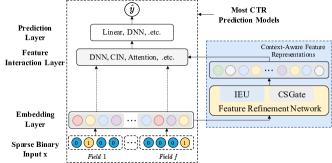
Figure 1. General paradigm of applying the proposed Feature Refinement Network in CTR prediction methods.

2. Related work

Many CTR prediction methods have achieved huge success by modeling feature interactions to enrich feature representations. Following recent works  (Luo et al., 2020; Cheng et al., 2020), we categorize CTR prediction methods into two types: traditional methods (Rendle, 2012; Juan et al., 2016; Pan et al., 2018; Yu et al., 2019; Lu et al., 2020) and deep learning-based methods (Cheng et al., 2016; Guo et al., 2017; Lian et al., 2018; Wang et al., 2021b; Song et al., 2019; Cheng et al., 2020; Zhao et al., 2021a, b). FM (Rendle, 2012) is one of the widely used traditional CTR prediction methods. Due to its effectiveness, many works have been proposed based on it  (Juan et al., 2016; Pan et al., 2018; Yu et al., 2019; Lu et al., 2020). However, these methods cannot capture high-order feature interactions. To address this issue, many deep learning-based methods were proposed to capture more complex feature interactions. Wide&Deep (WDL) (Cheng et al., 2016) jointly trains the wide linear unit and Multi-layer Perception (MLP) to combine the benefits of memorization and generalization. DeepFM  (Guo et al., 2017) replaces the wide part of WDL with FM to alleviate manual efforts in feature engineering. Based on DeepFM, xDeepFM (Lian et al., 2018) design a novel Compressed Interaction Network (CIN) to model high-order feature interactions explicitly. AutoInt (Song et al., 2019) uses stacked multi-head self-attention layers to model the feature interactions. Besides modeling feature interactions, XcrossNet (Yu et al., 2021) and AutoDis (Guo et al., 2021) design various structures to learn feature embedding for numerical features. Intuitively, each feature should have different representations based on its varying roles in different instances when we make predictions. However, the above methods only learn a fixed representation for each feature without considering the varying importance of each feature under different contexts, resulting in inferior performance.

Several recent CTR prediction methods  (Yu et al., 2019; Lu et al., 2020; Huang et al., 2019) attempted to learn vector-level weights for feature representations to address the fixed feature representation issue. IFM (Yu et al., 2019) and DIFM (Lu et al., 2020) propose Factor Estimating Network (FEN) and Dual-FEN to improve FM by learning vector-level weights for different feature representations. Similarly, FiBiNET  (Huang et al., 2019) uses Squeeze-and-Excitation network (SENET) (Hu et al., 2018) to extract informative features by reweighing the original features. However, only assigning vector-level weights to the same feature in different instances causes the learned representations of the same feature to have strictly linear relationships. However, it is unreasonable to only produce linear transformations to refine the fixed feature representations, because they are not flexible enough to capture the varying importance of each feature under different contexts. Recently, EGate (Huang et al., 2020) applied an independent MLP for each feature to learn bit-level weights. Nevertheless, the representations of the same features are still fixed, as it only transforms the representation space.

As summarized in Table 1, our method is related to but fundamentally different from existing methods because we learn both bit-level weights applied in original feature embedding and complementary features to ensure that FRNet can generate more flexible nonlinear context-aware feature representations.

Table 1. The connection and difference between FRNet and similar module. ✔—✗means totally—not met, respectively.

Module (Model)	Granularity	Context-Aware	Nonlinear
FEN (IFM(Yu et al., 2019))	Vector	✔	✗
Dual-FEN (DIFM (Lu et al., 2020))	Vector	✔	✗
SENET (FiBiNET (Huang et al., 2019))	Vector	✔	✗
EGate (GateNet (Huang et al., 2020))	Bit	✗	✗
FRNet-Vec (Ours)	Vector	✔	✔
FRNet (Ours)	Bit	✔	✔

3. Preliminaries

CTR prediction is a binary classification task on sparse multi-field categorical data (Pan et al., 2021; Huang et al., 2019; Yu et al., 2021). Suppose there are $f$ different fields and $n$ features, each field may contain multiple features but each feature only belongs to one field. Each instance for CTR prediction can be represented by $\left\{\mathbf{x}_{i},y_{i}\right\}$, where $\mathbf{x}_{i}$ is a sparse high-dimensional vector represented by one-hot encoding and $y_{i}\in{\{0,1\}}$ (click or not) is the true label, e.g.,

(1) $$\mathbf{x}_{i}=\underset{Item=Computer\,\,}{\underbrace{\left(0,...,1,0\right)}}\underset{Color=White\,\,}{\underbrace{\left(1,...,0,0\right)}}\mathbf{...}\underset{Gender=Female}{\underbrace{\left(1,0\right).}}$$

CTR prediction models aim to approximate the probability $P(y_{i}|\mathbf{x}_{i})$ for each instance. According to (Wei et al., 2021; Wang et al., 2021a), most recent CTR prediction methods follow the design paradigm below (as shown in Figure 1):

Embedding layer. It transforms the sparse high-dimensional features $\mathbf{x}_{i}$ into a dense low-dimensional embedding matrix $\mathbf{E}=[\mathbf{v}_{1};\mathbf{v}_{2};...;\mathbf{v}_{f}]\in\mathbb{R}^{f\times d}$, where $d$ is the dimension size of each field. Each feature has a fixed-length representation $\mathbf{v}_{i}$.

Feature interaction layer. In CTR prediction methods, the most critical design is the feature interaction layer, which uses various types of interaction operations to capture arbitrary-order feature interactions, such as MLP (Guo et al., 2017; Cheng et al., 2016), Cross Network (Wang et al., 2021b, 2017) and transformer layer (Li et al., 2020a; Song et al., 2019), etc. The output of feature interaction layer is a compact representation $\mathbf{q}_{i}$ based on embedding matrix $\mathbf{E}$.

Prediction layer. Finally, a prediction layer (usually a linear regression or MLP module) produces the final prediction probability $\sigma(\hat{y_{i}})\in(0,1)$ based on the representations $\mathbf{q}_{i}$, where $\sigma(x)=1/(1+\exp(-x))$ is the sigmoid function. And, a common loss function for CTR prediction tasks is the cross entropy loss as follows:

(2) $$\textstyle loss=-\frac{1}{N}\sum_{i=1}^{N}{y_{i}}\log\left(\sigma\left(\hat{y}_{i}\right)\right)+\left(1-y_{i}\right)\log\left(1-\sigma\left(\hat{y}_{i}\right)\right),$$

where $N$ is total number of training instances.

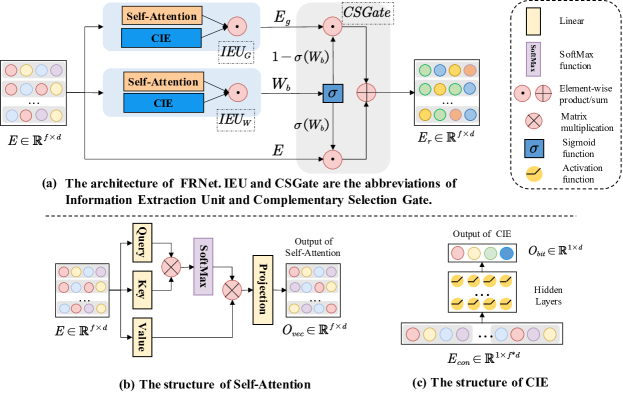
Figure 2. Architectures of Feature Refinement Network (FRNet), Self-Attention and Contextual Information Extractor (CIE).

4. Feature Refinement Network

In this section, we introduce the details of FRNet. As depicted in Figure 2 (a), FRNet contains two key components:

• Information Extraction Unit (IEU), which can capture contextual information and cross-feature relationships to guide context-aware feature refinement.

• Complementary Selection Gate (CSGate), which can adaptively integrate the original and complementary feature representations with bit-level weights to achieve context-aware feature representation learning.

4.1. Information Extraction Unit (IEU)

IEU consists of three essential components: 1) the Self-Attention unit, which is deployed to capture explicit cross-feature relationships among co-occurring features; 2) Contextual Information Extractor (CIE), which aims to encode the contextual information under different contexts; and 3) Integration unit, which integrates the information from the Self-Attention unit and CIE. In addition, we use two IEUs for two purposes: $IEU_{W}$ learns bit-level weights, and $IEU_{G}$ produces complementary feature representations.

4.1.1. Self-Attention unit

We adopt self-attention (Vaswani et al., 2017) to identify the most relevant features to each specific feature in instances. For instance, in {female, red, lipstick, workday}, the most relevant features to “female” are “red” and “lipstick”. The self-attention module first calculates importance among all feature pairs and generates new representations by computing the weighted sum of relevant features. To achieve higher efficiency, we simplify the structure of self-attention as depicted in Figure 2 (b). More detailed, we first map the input matrix $\mathbf{E}$ into three different matrices:

(3) $$\mathbf{Q},\mathbf{K},\mathbf{V}=\mathbf{EW^{Q}},\mathbf{EW^{K}},\mathbf{EW^{V}},$$

where $\mathbf{W^{Q}}$, $\mathbf{W^{K}}$, $\mathbf{W^{V}}\in\mathbb{R}^{d\times d_{k}}$ are transformation matrices, and $d_{k}$ is the attention size. Then, we obtain the attention matrix on Value ($\mathbf{V}$) by applying the dot product of Query ($\mathbf{Q}$) and Key ($\mathbf{K}$) with a Softmax function as follows:

(4) $$Attention(\mathbf{Q},\mathbf{K},\mathbf{V})=SoftMax(\mathbf{QK^{T}})\mathbf{V}\in\mathbb{R}^{f\times d_{k}}.$$

Finally, we transform the dimension of output matrix to be the same as the input by a projection matrix $\mathbf{W^{P}}\in\mathbb{R}^{d_{k}\times d}$ . The output ($\mathbf{O_{vec}}$) of the self-attention module can be summarized as follows:

(5) $$\mathbf{O_{vec}}=Attention(\mathbf{Q,K,V})\mathbf{W^{P}}\in\mathbb{R}^{f\times d}.$$

The self-attention mechanism can achieve partially context-aware feature representation learning by capturing the cross-feature relationships among all feature pairs to refine the feature representation under different contexts. However, self-attention only utilizes partial contextual information represented by pair-wise feature interactions and thus fails to utilize complete contextual information to guide feature refinement. In other words, self-attention yields similar feature representations for the same features in different instances, as shown in our studies (Section 5.7).

4.1.2. Contextual Information Extractor

The contextual information in each instance is implicitly contained in all features. Hence, we need to ensure that all features contribute to the contextual information in each instance. Since the contextual information is usually not very complicated, MLP is a simple yet effective choice to extract contextual information as shown in the experiments (Section 5.4). In detail, we first concatenate the original feature representations into $\mathbf{E_{con}}$ as the input.

Then, each layer of the MLP is obtained as follows:

(6) $$\mathbf{h}_{l+1}=PReLU(\mathbf{W}_{l}\mathbf{h}_{l}+b_{l}),$$

where $\mathbf{h}_{l}\in\mathbb{R}^{n_{l}}$, $\mathbf{h}_{l+1}\in\mathbb{R}^{n_{l+1}}$ are the $l$-th and ${(l+1)}$-th hidden layer, and $\mathbf{h}_{0}=\mathbf{E_{con}}\in\mathbb{R}^{1\times(f*d)}$. $\mathbf{W}_{l}\in\mathbb{R}^{n_{l+1}\times n_{l}}$, $b_{l}$ are the learnable parameters for the $l$-th deep layer. PReLU(·) is the PReLU (He et al., 2015) function. In the last hidden layer, we project the dimension of contextual information vector to $d$ (the dimension of embedding size), and compute the contextual information vector $\mathbf{O_{bit}}$ as follows:

(7) $$\mathbf{O_{bit}}=PReLU(\mathbf{W}_{L}\mathbf{h}_{L}+b_{L})\in\mathbb{R}^{1\times d},$$

where $\mathbf{W}_{L}\in\mathbb{R}^{d\times n_{L-1}}$, $b_{L}$ are the parameters of the last layer. Since $\mathbf{O}_{bit}$ compresses all information from $\mathbf{E_{con}}$, it can represent the contextual information within the specific instance. Intuitively, contextual information $\mathbf{O_{bit}}$ is unique for each instance, as different instances contain different features.

4.1.3. Integration unit

After obtaining the contextual information $\mathbf{O_{bit}}$, we directly use $\mathbf{O_{bit}}$ to weigh the feature representation $\mathbf{O_{vec}}$. As illustrated in Figure 3 (a), it is calculated as follows:

(8) $$\mathbf{O_{IEU}}=\mathbf{O_{vec}}\odot\mathbf{O_{bit}}\in\mathbb{R}^{f\times d}.$$

$\odot$ is the element-wise product. $\mathbf{O_{vec}}$ is the feature representation from self-attention module which captures cross-feature relationships, and $\mathbf{O_{bit}}$ enables each feature representation to be aware of the contextual information. Equation 8 ensures each feature can have significantly different representations in different instances.

As shown in Figure 2 (a), we deploy two independent IEUs: (1) $IEU_{W}$ learns bit-level weights; (2) $IEU_{G}$ produces complementary features. Specifically, their outputs are represented as follows:

(9) $$\mathbf{E_{g}}=\mathbf{IEU_{G}(E)}\in\mathbb{R}^{f\times d},~{}~{}\mathbf{W_{b}}=\mathbf{IEU_{W}(E)}\in\mathbb{R}^{f\times d}.$$

We will present more details of Equation 9 in the next subsection.

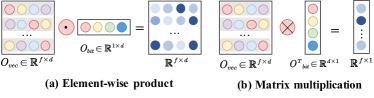
Figure 3. The operations to integrate the outputs of self-attention and CIE units.

4.2. Complementary Selection Gate (CSGate)

In CSGate, we design a novel gate mechanism to control information flow and select important information from the original and complementary features with bit-level weights. As shown in Figure 2 (a), CSGate has three different inputs from three channels: 1) complementary feature representations $\mathbf{E_{g}}$; 2) weight matrix $\mathbf{W_{b}}$; and 3) original feature representations $\mathbf{E}$. The output of CSGate is the context-aware feature representation:

(10) $$\mathbf{E}_{\mathbf{r}}=\underset{Selected\,\,features\,\,}{\underbrace{\mathbf{E}\odot\sigma\left(\mathbf{W_{b}}\right)}}+\underset{Complementary\ features\,\,}{\underbrace{\mathbf{E}_{\mathbf{g}}\odot\left(1-\sigma\left(\mathbf{W_{b}}\right)\right)}},$$

where $\sigma(\cdot)$ is the sigmoid function. $\mathbf{E_{r}}\in\mathbb{R}^{f\times d}$ has the same dimensions as $\mathbf{E}$. Specifically, Equation (10) contains two parts of features: selected features and complementary features. Those two parts are connected by the selection gate $\sigma(\mathbf{W_{b}})$.

Selected Features are the selected important information from original feature representations at bit-level. Specifically, each element in $\sigma(\mathbf{W_{b}})$ measures the importance of the corresponding element in the original feature representation $\mathbf{E}$, where the probability of selecting the specific element is between 0 and 1. Thus, we can learn nonlinear context-aware feature representations. Compared with previous works (Lu et al., 2020; Yu et al., 2019; Huang et al., 2019), the learned weight matrix $\sigma(\mathbf{W_{b}})$ have two advantages: 1) it contains cross-feature relationships and contextual information simultaneously, which enables to learn context-aware representations for the same feature in different instances; and 2) introducing the bit-level weights to the original feature representations can achieve more flexible and fine-grained feature refinement than previous linear transformations.

Complementary Features are the complementary information that aims to further enhance the expressive capacity of context-aware feature representations. Existing methods (Yu et al., 2019; Huang et al., 2019; Lu et al., 2020) only assign weights to original features without considering the unselected information. However, we believe the unselected features may still help CTR prediction in a different way. Hence, we propose to leverage $\mathbf{E_{g}}$ with its weight $1-\sigma(\mathbf{W_{b}})$ as the other part of the final context-ware feature representations. In particular, the gate $\sigma(\mathbf{W_{b}})$ achieves adaptive balance between the selected features and complementary features in bit level.

In summary, FRNet generates context-aware feature representation by three steps: 1) generating complementary feature representations using $IEU_{G}$; 2) calculating bit-level weight matrix by $IEU_{W}$; and 3) leveraging the CSGate to generate context-aware feature interactions by integrating original features representations and complementary feature representations by bit-level weights.

5. Experiments

5.1. Experimental Setup

5.1.1. Datasets

We conduct experiments on four popular datasets:

Criteo is the most well-known industrial benchmark dataset for CTR prediction, which includes 26 anonymous categorical fields and 13 numerical fields. We discretize numerical features and transform them into categorical features by log transformation. And following  (Yang et al., 2020), we use the last 5 million records for testing. Meanwhile, we remove the features appeared less than 10 times and treat them as a dummy feature “$\langle unknown\rangle$”.

Malware is published in the Microsoft Malware prediction, which contains 81 different fields. This task can be transformed as a binary classification problem like a CTR prediction task (Wang et al., 2021a).

Frappe contains app usage logs from users under different contexts (e.g., daytime, location). The target value indicates whether the user has used the app under the context (Xiao et al., 2017).

MovieLens contains user tagging records on movies. Each instance contains three fields: user ID, movie ID, tag. The targeted value denotes whether a user has assigned a tag to a movie (Xiao et al., 2017).

The statistics of these four datasets are summarized in Table 2.

5.1.2. Evaluation Metrics

To evaluate the performance of CTR prediction methods, we adopt AUC (Area under the ROC curve) and Logloss (binary cross-entropy loss) as the evaluation metrics (Chen et al., 2021; Wang et al., 2021a). Note that slightly higher AUC or lower Logloss, e.g., at 0.001 level, can be regarded as significant improvement in CTR prediction tasks (Chen et al., 2021; Luo et al., 2020; Wang et al., 2021b; Cheng et al., 2016; Huang et al., 2019; Lian et al., 2018; Li et al., 2020b).

5.1.3. Compared Models

We apply FRNet into FM (Rendle, 2012), which is called $FM_{FRNet}$. We compare $FM_{FRNet}$ with three types of methods: 1) FM-based methods, which capture second- or higher-order feature interactions, including FM (Rendle, 2012), IFM (Yu et al., 2019), DIFM (Lu et al., 2020); 2) deep learning-based methods, which model high-order feature interactions, including NFM (He and Chua, 2017), IPNN (Qu et al., 2018), OPNN (Qu et al., 2018), CIN (Lian et al., 2018), FINT (Zhao et al., 2021a); and 3) ensemble methods, which adopt multi-tower feature interaction structures to integrate different types of methods, including WDL (Cheng et al., 2016), DCN (Wang et al., 2017), DeepFM (Guo et al., 2017), xDeepFM (Lian et al., 2018), FiBiNET (Huang et al., 2019), AutoInt+ (Song et al., 2019), AFN+ (Cheng et al., 2020), NON (Luo et al., 2020), TFNET (Wu et al., 2020), FED (Zhao et al., 2020), and DCN-V2 (Wang et al., 2021b). We do not present the results of classical methods, including LR (Richardson et al., 2007), GBDT (He et al., 2014), CCPM (Gehring et al., 2017), FFM (Juan et al., 2016), AFM (Xiao et al., 2017), FwFM (Pan et al., 2018), CrossNet (Wang et al., 2017), FNN  (Zhang et al., 2016), because more recent methods (e.g., AFN+ (Cheng et al., 2020), FiBiNET (Huang et al., 2019), DCN-V2 (Wang et al., 2021b)) have outperformed these methods in their experiments.

To demonstrate the effectiveness of the bit-level weights in FRNet, we design a variant of FRNet named FRNet-Vec, where FRNet-Vec only learns the vector-level weights in IEU and keep the other parts the same as FRNet. As shown in Figure 3 (b), the weight matrix $\mathbf{W}_{v}$ in FRNet-Vec is calculated by:

(11) $$\mathbf{W}_{v}=\mathbf{O_{vec}}\otimes\mathbf{O^{T}_{bit}}\in\mathbb{R}^{f\times 1}.$$

Each element in $\sigma(\mathbf{W}_{v})$ measures the importance of each feature representations in original embedding $\mathbf{E}\in\mathbb{R}^{f\times d}$.

Table 2. Statistics of four datasets used in this paper.

Datasets	Positive	#Training	#Validation	#Testing	#Fields	#Features
Criteo	26%	35,840,617	5,000,000	5,000,000	39	1,086,810
Malware	50%	7,137,187	892,148	892,148	81	976,208
Frappe	33%	202,027	57,722	28,860	10	5,382
MovieLens	33%	1,404,801	401,372	200,686	3	90,445

5.1.4. Implementation Details.

We implement our method with Pytorch. All models are learned by optimizing the Cross-Entropy loss with Adam (Kingma and Ba, 2015) optimizer. We implement the Reduce-LR-On-Plateau scheduler during the training process to reduce the learning rate by a factor of 10, when the given metric stops improving in four consecutive epochs. The default learning rate is 0.001. We use early stop to avoid overfitting when the AUC on the validation set stops improving. The mini-batch size is set to 4096. The embedding size is 10 for Criteo and Malware and 20 for Frappe and MovieLens, respectively. Following previous works (Huang et al., 2019; Cheng et al., 2020; Guo et al., 2017; Song et al., 2019), we employ the same neural structure (i.e., 3 layers, 400-400-400) for the models that involve MLP for a fair comparison. All activation functions are ReLU unless otherwise specified, and the dropout rate is set to 0.5. In FRNet, the dimension of MLP in the CIE is set to 128. For other methods, we take the optimal settings from the original papers.

To ensure fair comparison, we run all experiments five times by changing random seeds and report the averaged results. We observe that all the standard deviations of our method are in the order of 1e-4, indicating that our results are very stable. We further perform two-tailed t-test to verify the statistical significance in comparisons between our method and the best baseline methods.

Table 3. Overall accuracy comparison in the four datasets. $\Delta_{AUC}$ and $\Delta_{Logloss}$ are calculated to indicate averaged performance boost compared with the best baseline (DCN-V2) over the four datasets. Two tailed t-test: $\star:p<10^{-2}$, $\star\star:p<10^{-4}$.

Model Class	Datasets	Criteo		Malware		Frappe		MovieLens		$\Delta_{AUC}$ $\uparrow$	$\Delta_{Logloss}$ $\downarrow$
	Model	AUC	Logloss	AUC	Logloss	AUC	Logloss	AUC	Logloss
Second-Order	FM	0.8028	0.4514	0.7309	0.6052	0.9708	0.1934	0.9391	0.2856	-1.13%	+0.0167
	IFM	0.8066	0.4470	0.7389	0.5969	0.9765	0.1896	0.9471	0.2853	-0.39%	+0.0125
	DIFM	0.8085	0.4457	0.7397	0.5954	0.9788	0.1860	0.9490	0.2459	-0.19%	+0.0011
High-Order	NFM	0.8057	0.4483	0.7352	0.5988	0.9746	0.1915	0.9437	0.2945	-0.68%	+0.0161
	IPNN	0.8088	0.4454	0.7404	0.5945	0.9791	0.1759	0.9490	0.2785	-0.15%	+0.0064
	OPNN	0.8096	0.4446	0.7408	0.5840	0.9795	0.1805	0.9497	0.2704	-0.08%	+0.0027
	CIN	0.8082	0.4459	0.7395	0.5967	0.9776	0.2010	0.9483	0.2808	-0.26%	+0.0139
	FINT	0.8090	0.4452	0.7402	0.5953	0.9791	0.1921	0.9498	0.2674	-0.13%	+0.0078
Ensemble	WDL	0.8068	0.4474	0.7392	0.5982	0.9776	0.1895	0.9403	0.3045	-0.52%	+0.0177
	DCN	0.8091	0.4452	0.7403	0.5944	0.9789	0.1814	0.9458	0.2685	-0.23%	+0.0052
	FiBiNET	0.8093	0.4450	0.7405	0.5942	0.9787	0.1867	0.9471	0.2630	-0.19%	+0.0050
	DeepFM	0.8084	0.4458	0.7402	0.5944	0.9789	0.1770	0.9465	0.3079	-0.24%	+0.0141
	xDeepFM	0.8086	0.4456	0.7405	0.5940	0.9792	0.1889	0.9480	0.2889	-0.18%	+0.0122
	AutoInt+	0.8088	0.4456	0.7406	0.5939	0.9786	0.1890	0.9501	0.2813	-0.13%	+0.0103
	AFN+	0.8095	0.4447	0.7404	0.5945	0.9791	0.1824	0.9509	0.2583	-0.08%	+0.0028
	NON	0.8096	0.4446	0.7390	0.5956	0.9792	0.1813	0.9505	0.2625	-0.13%	+0.0038
	TFNet	0.8092	0.4449	0.7397	0.5948	0.9787	0.1942	0.9493	0.2714	-0.16%	+0.0091
	FED	0.8087	0.4458	0.7406	0.5942	0.9797	0.1802	0.9510	0.2576	-0.08%	+0.0022
	DCN-V2	0.8098	0.4443	0.7411	0.5935	0.9802	0.1783	0.9516	0.2527	-	-
Our Models	$FM_{FRNet-Vec}$	$0.8115^{\star\star}$	$0.4428^{\star\star}$	$0.7438^{\star\star}$	$0.5914^{\star\star}$	$0.9816^{\star\star}$	$0.1653^{\star}$	$0.9635^{\star\star}$	$0.2365^{\star\star}$	0.49%	-0.0082
	$FM_{FRNet}$	$\textbf{0.8120}^{\star\star}$	$\textbf{0.4424}^{\star\star}$	$\textbf{0.7445}^{\star\star}$	$\textbf{0.5909}^{\star\star}$	$\textbf{0.9830}^{\star\star}$	$\textbf{0.1607}^{\star\star}$	$\textbf{0.9679}^{\star\star}$	$\textbf{0.2278}^{\star}$	0.68%	-0.0118

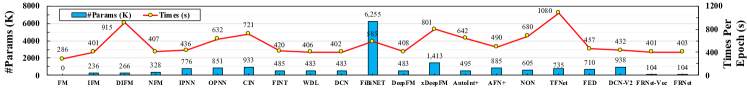
Figure 4. Efficiency comparisons of different algorithms in terms of Model Size and Run Time on the Criteo dataset. We only consider the parameters above the embedding layer (including LR part). We conduct experiments with one TITAN V GPU.

5.2. Overall Comparison

5.2.1. Effectiveness Comparison.

Table 3 summarizes the effectiveness of FRNet and all compared methods on the four datasets. Although FM has the worst performance, $FM_{FRNet}$ and $FM_{FRNet-Vec}$ statistically significantly outperform all compared methods. Specifically, $FM_{FRNet}$ outperforms FM by 1.15%, 1.86%, 1.26% and 3.07% in terms of AUC (1.99%, 2.36%, 16.91% and 20.23% in terms of Logloss) on four datasets, respectively, which demonstrates that learning context-aware feature representations is effective in CTR prediction. Meanwhile, the averaged performance boost ($\Delta_{AUC}$ and $\Delta_{Logloss}$) indicate the most strong generalization ability of $FM_{FRNet}$ and $FM_{FRNet-Vec}$ on four datasets. In addition, $FM_{FRNet}$ achieves better performance than $FM_{FRNet-Vec}$, which confirms that refining feature representations at bit-level is more effective. Most importantly, Table 3 indicates that learning context-aware feature representations by FRNet is more effective than other feature interaction techniques, e.g., the ones in xDeepFM, NON, and DCN-V2.

5.2.2. Efficiency Comparison.

We compare the model size and run time of different methods in Figure 4. Generally, FM-based methods have fewer parameters than high-order or ensemble methods. Specifically, $FM_{FRNet}$ only increases 104K learning parameters over FM. As a comparison, DIFM and xDeepFM increase 266K and 483K learning parameters over FM, respectively. Meanwhile, they are relatively time-consuming, as they consist of complicated structures, e.g., Dual-FEN and CIN. We also observe from Figure 4 that $FM_{FRNet}$ is comparable to IFM and DCN, and has fewer model parameters and is more efficient than all other baseline methods. Notably, compared with the best-performing baseline DCN-V2, $FM_{FRNet}$ has fewer model parameters, faster training speed and better performance.

Table 4. Compatibility comparison between FRNet and other four modules over SOTA CTR prediction methods.

Datasets	Modules	BASE		SENET (FiBiNET)		EGate (GateNet)		FEN (IFM)		Dual-FEN (DIFM)		FRNet (Ours)
	Models	AUC	Logloss	AUC	Logloss	AUC	Logloss	AUC	Logloss	AUC	Logloss	AUC	Logloss
Criteo	FM	0.8028	0.4514	0.8073	0.4467	0.8058	0.4482	0.8066	0.4470	0.8085	0.4457	0.8120	0.4424
	AFM	0.7999	0.4535	0.8048	0.4486	0.7925	0.4601	0.7951	0.4576	0.7924	0.4600	0.8116	0.4427
	NFM	0.8057	0.4483	0.8063	0.4476	0.8060	0.4479	0.8063	0.4474	0.8080	0.4461	0.8120	0.4425
	DeepFM	0.8084	0.4458	0.8089	0.4453	0.8085	0.4457	0.8085	0.4459	0.8094	0.4448	0.8118	0.4426
	xDeepFM	0.8086	0.4456	0.8093	0.4451	0.8100	0.4442	0.8087	0.4455	0.8101	0.4443	0.8110	0.4434
	IPNN	0.8088	0.4454	0.8100	0.4442	0.8104	0.4438	0.8102	0.4441	0.8094	0.4450	0.8115	0.4428
	FiBiNET	0.8093	0.4450	0.8093	0.4450	0.8102	0.4440	0.8102	0.4439	0.8104	0.4436	0.8119	0.4425
	Avg. Imp	-	-	0.22%	0.40%	0.00%	0.04%	0.04%	0.12%	0.08%	0.18%	0.68%	1.15%
Frappe	FM	0.9708	0.1934	0.9764	0.1863	0.9515	0.3134	0.9765	0.1896	0.9788	0.1860	0.9830	0.1607
	AFM	0.9606	0.2483	0.9620	0.2453	0.9477	0.2733	0.9487	0.2704	0.9698	0.2417	0.9803	0.1831
	NFM	0.9746	0.1915	0.9787	0.1794	0.9754	0.1860	0.9774	0.1778	0.9785	0.1758	0.9822	0.1620
	DeepFM	0.9789	0.1770	0.9813	0.1642	0.9808	0.1682	0.9817	0.1625	0.9796	0.1727	0.9836	0.1594
	xDeepFM	0.9792	0.1889	0.9817	0.1629	0.9805	0.1694	0.9814	0.1679	0.9807	0.1715	0.9824	0.1653
	IPNN	0.9791	0.1759	0.9812	0.1639	0.9805	0.1667	0.9815	0.1634	0.9809	0.1650	0.9828	0.1597
	FiBiNET	0.9787	0.1867	0.9787	0.1867	0.9803	0.1674	0.9798	0.1736	0.9805	0.1648	0.9821	0.1635
	Avg. Imp	-	-	0.27%	8.64%	-0.37%	-2.31%	0.07%	7.84%	0.40%	9.32%	0.80%	17.43%

5.3. Compatibility Analysis

To confirm the compatibility of FRNet, we apply FRNet in seven CTR prediction methods. Meanwhile, we compare FRNet with additional four modules proposed by recent works which assign different weights to the original feature representations, such as SENET (Huang et al., 2019), EGate (Huang et al., 2020), FEN (Yu et al., 2019), and Dual-FEN (Lu et al., 2020). Same as FRNet, we place the above modules after the embedding layer as mentioned in section 3. In FiBiNET (Huang et al., 2019), we replace its SENET with other modules to refine the features. Table 4 shows their performance, and we can make the following conclusions: (1) Learning context-aware feature representations is vital for improving the performance of CTR prediction. Compared with base models, the average improvements (Avg. Imp) of FRNet are 0.68% and 0.80% in terms of AUC (1.15% and 17.43% in terms of Logloss) on Criteo and Frappe, which demonstrates the high effectiveness and compatibility of FRNet. (2) FRNet significantly outperforms the other four modules when applied to base models. FRNet is the only module that can enhance the performance of all seven base models. In contrast, the other four modules may reduce the performance of CTR prediction in some of the datasets or base models. For instance, Applying EGate in FM and AFM achieves poor performance on the Frappe dataset. These phenomena indicate that these model-specific feature refinement modules are with limited compatibility. On the contrary, FRNet has strong compatibility and can be applied in a wide range of CTR prediction models to enhance their performance.

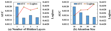
Figure 5. Impact of hyper-parameters on Criteo.

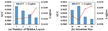
Figure 6. Impact of hyper-parameters on Frappe.

5.4. Hyper-parameter Study

We analyze the impact of hyper-parameters in FRNet, including the number of hidden layers in MLP, the attention size $d_{k}$ of the Self-Attention. For the sake of convenience, we change the hyper-parameters in $IEU_{G}$ and $IEU_{W}$ simultaneously. Note that we only change one hyper-parameter and keep the other one fixed in each experiment.

Number of Hidden Layers. Figure 5 (a) and Figure 6 (a) show the impact of the number of hidden layers at bit-level unit. For Criteo and Frappe, the most appropriate number of hidden layers is 1. This confirms that the contextual information is not very complicated and a shallow MLP is strong enough to encode contextual information from each instance.

Attention Size. As shown in Figure 5 (b) and Figure 6 (b), the best attention size for Criteo and Frappe are 10 and 20, respectively. For Criteo, the performance decreases when we increase the attention size. Coincidentally, the dimension of the embedding for Criteo and Frappe are exactly 10 and 20. It may be a good trick to set the attention size to be the same as the embedding dimension.

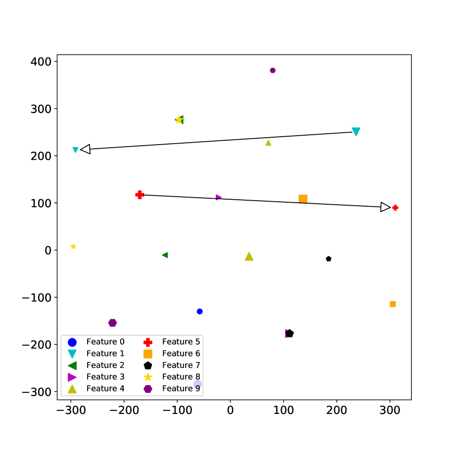
(a) EGate

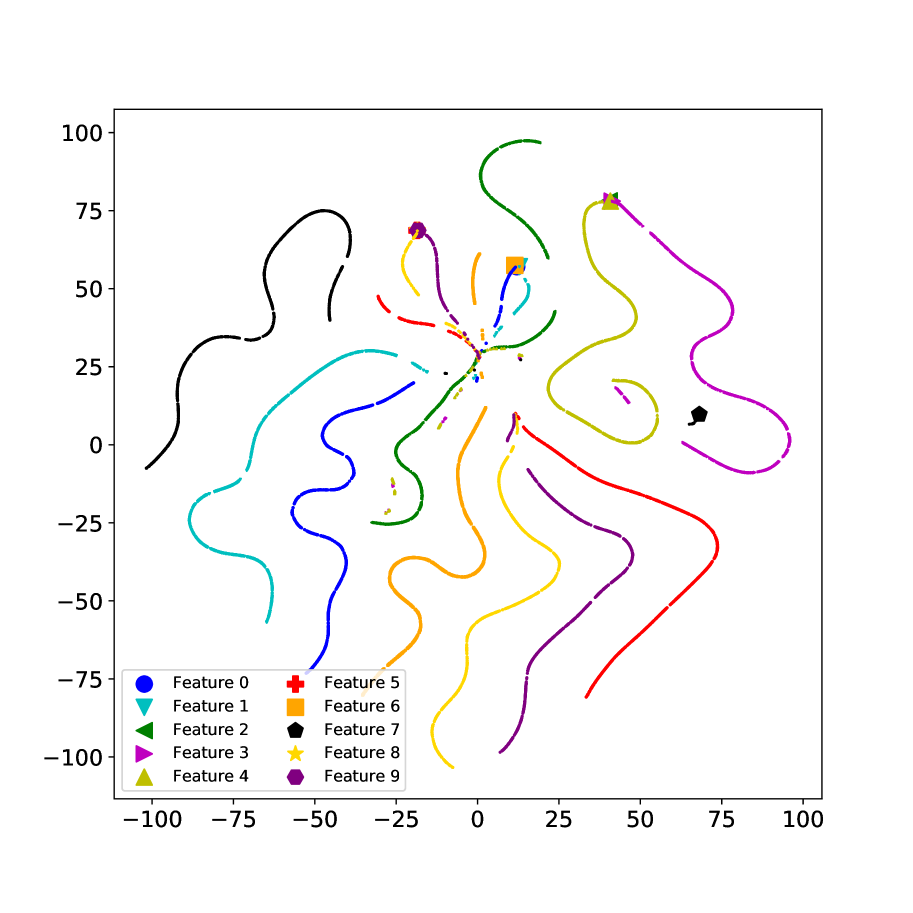
(b) DIFM

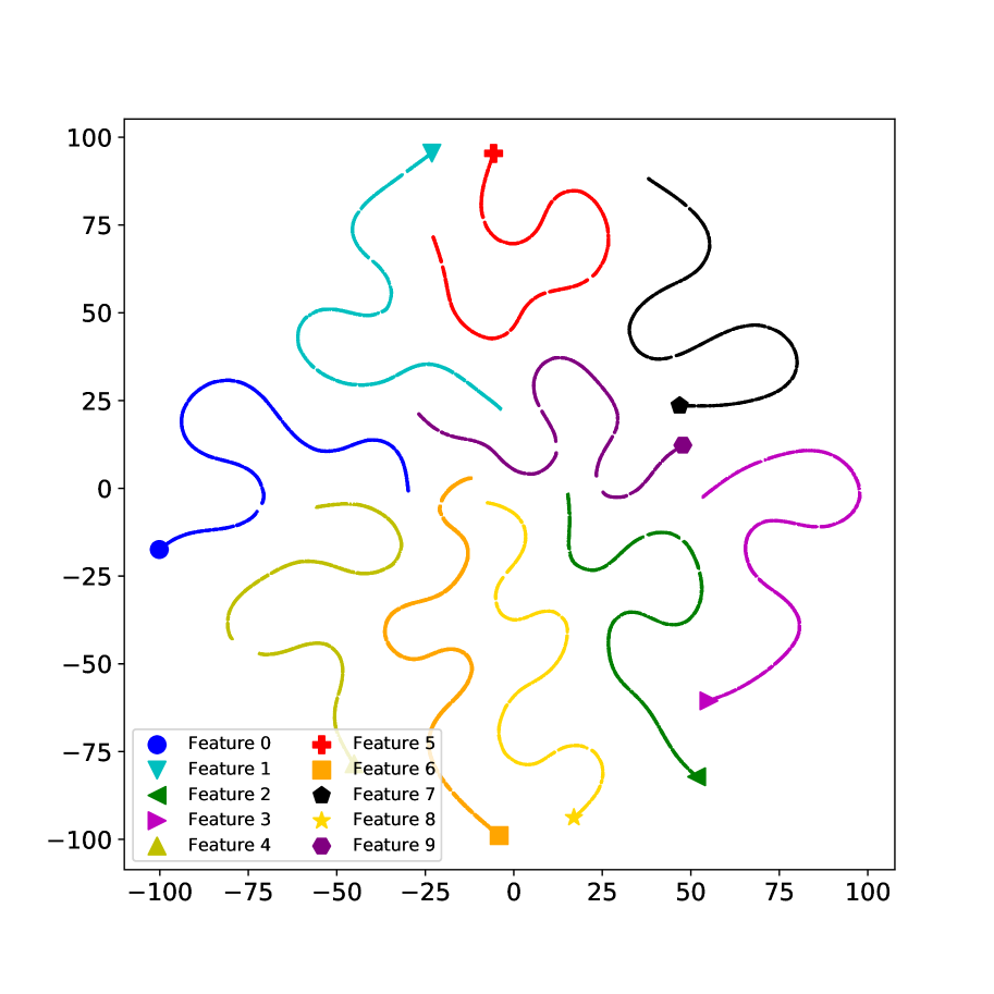
(c) Variant #6

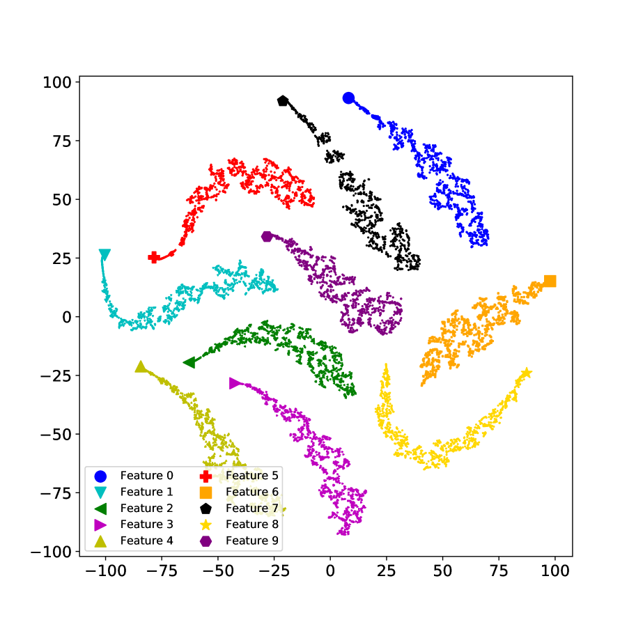
(d) FRNet-Vec

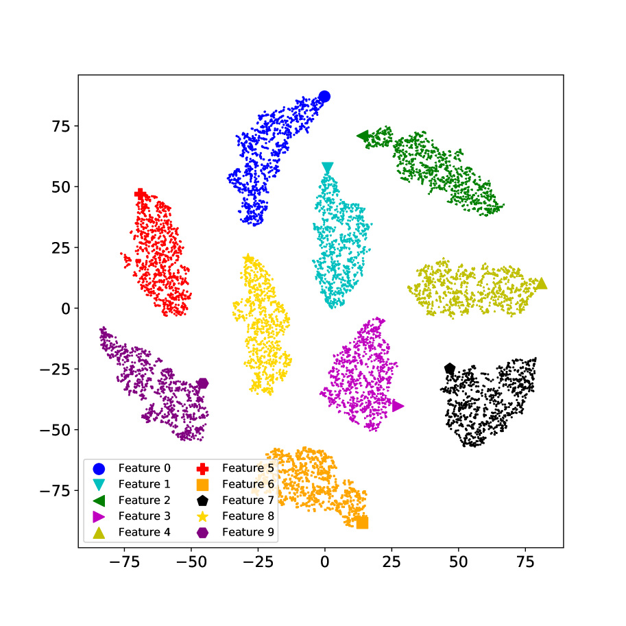
(e) FRNet

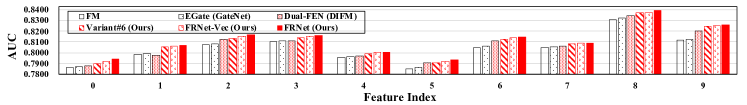
(f) Test AUC on Corresponding Subsets of each feature. Each subset contains 1,000 instances.

Figure 7. Visualization of context-aware feature representations for 10 features in same field. We randomly choose 1000 instances for each feature. Hence, each feature has an original representation and 1,000 context-aware feature representations.

5.5. Ablation Study

Here, we conduct experiments on Criteo and Frappe to prove that each component or design in FRNet plays an essential role in improving the performance of CTR prediction. As shown in Table 5, we use the equations to describe how to compute $\mathbf{E}_{r}$ base on $\mathbf{E}$ by removing or replacing one of the components in FRNet. Especially, variant #4 denotes that we only use a self-attention unit in $IEU_{G}$ and $IEU_{W}$. From Table 5, we can make the following conclusions:

(1) Learning context-aware feature representations is reasonable. It can be proved that all variants of the FRNet successfully improve the performance of FM on these two datasets;

(2) Cross-feature relationships and contextual information are essential. With cross-feature relationships, variant #2 outperforms #1. Meanwhile, #13 outperforms #4, and #3 outperforms #2, respectively, which shows the effectiveness of contextual information within different instances;

(3) Assigning weights to original features is valid. In #5, we remove $IEU_{W}$ and then directly add $\mathbf{E}$ and $\mathbf{E_{g}}$. We can find that #10 and #11 outperform #5, where the learned weights matrix $\mathbf{W_{b}}$ or $\mathbf{W_{v}}$ successfully selects important information from $\mathbf{E}$. In addition, #6 and #7 outperform #1, from which we can draw the same conclusion;

(4) Learning bit-level weights is more effective than learning vector-level weights. The variants learning bit-level weights (#7, #9, #11, #13) consistently outperform those corresponding variants learning vector-level weights (#6, #8, #10, #12) respectively, which verifies that learning more fine-grained weights for selecting information is more effective. Intuitively, each element of one feature representation has a specific semantic meaning, so we should give them different weights instead of treating them equally;

(5) Complementary Features are crucial. Variants #6 and #7 only learn feature representations from the original feature representations. After adding $\mathbf{E}_{g}$, #10 and #11 outperforms #6 and #7 respectively. Furthermore, we observe that #12 and #13 outperform #10 and #11, as we assign weights $1-\sigma(\mathbf{W_{b}})$ to $\mathbf{E}_{g}$, which verifies that assigning weights to complementary features is reasonable. In summary, it is reasonable that the CSGate integrates $\mathbf{E}$ and $\mathbf{E}_{g}$ with $\mathbf{W_{b}}$. As a comparison, we adopt the idea of Residual Network (He et al., 2016) in variants #8 and #9 (i.e, adding original representations $\mathbf{E}$), which is also used in DIFM (Lu et al., 2020). However, the performance of #8 and #9 are worse than #6 and #7. The reason is that residual network aims to add the original feature representations to the final feature representations, which might not be enough for CTR prediction.

Table 5. Ablation study of FRNet. $\mathbf{E}$, $\mathbf{E}_{g}$ and $\mathbf{E}_{r}$ denote the original, complementary and context-aware feature representations respectively. $\mathbf{W}_{b}$ and $\mathbf{W}_{v}$ denote bit-level and vector-level weights. $\mathbf{O}_{vec}$ is the output of self-attention unit.

Comment/Equation	Datasets	Criteo		Frappe
	Variant	AUC	Logloss	AUC	Logloss
FM ($\mathbf{E_{r}}=\mathbf{E}$)	#1	0.8028	0.4514	0.9708	0.1934
$\mathbf{E_{r}}=\mathbf{O_{vec}}$	#2	0.8056	0.4483	0.9717	0.1912
$\mathbf{E_{r}}=\mathbf{E_{g}}$	#3	0.8071	0.4470	0.9744	0.1897
Removing CIE	#4	0.8073	0.4468	0.9754	0.1878
$\mathbf{E_{r}}=\mathbf{E}+\mathbf{E_{g}}$	#5	0.8090	0.4452	0.9778	0.1821
$\mathbf{E_{r}}=\mathbf{E}\odot\sigma(\mathbf{W_{v}})$	#6	0.8110	0.4443	0.9793	0.1713
$\mathbf{E_{r}}=\mathbf{E}\odot\sigma(\mathbf{W_{b}})$	#7	0.8113	0.4437	0.9797	0.1697
$\mathbf{E_{r}}=\mathbf{E}\odot\sigma(\mathbf{W_{v}})+\mathbf{E}$	#8	0.8093	0.4452	0.9791	0.1739
$\mathbf{E_{r}}=\mathbf{E}\odot\sigma(\mathbf{W_{b}})+\mathbf{E}$	#9	0.8098	0.4449	0.9794	0.1726
$\mathbf{E_{r}}=\mathbf{E}\odot\sigma(\mathbf{W_{v}})+\mathbf{E_{g}}$	#10	0.8110	0.4433	0.9798	0.1696
$\mathbf{E_{r}}=\mathbf{E}\odot\sigma(\mathbf{W_{b}})+\mathbf{E_{g}}$	#11	0.8114	0.4430	0.9804	0.1689
FRNet-Vec	#12	0.8115	0.4428	0.9816	0.1653
FRNet	#13	0.8120	0.4424	0.9830	0.1607

5.6. Visualization of Feature Representations

5.6.1. Visualization Analysis.

To better understand the effectiveness of context-aware feature representations, we first randomly select 10 features from the same field and choose 1,000 instances for each feature from Criteo. Then, we learn the 1,000 feature representations by: (a) EGate, (b) DIFM, (c) Variant#6, (d) FRNet-Vec and (e) FRNet. Finally, we visualizes their feature representations with t-SNE (Van der Maaten and Hinton, 2008) in Figure 7. Each color in Figure 7 represents the original representation of one feature (denoted by the largest symbols, e.g., dots, squares, etc.) and 1,000 different context-aware feature representations in different instances (denoted by smaller symbols). Variant #6 is defined in Section 5.5, which learns vector-level weights for $\mathbf{E}$ by $IEU_{W}$. Note that we compress the size of feature representations to 2 in this part for the sake of visualization. As shown in Figure 7, each feature can learn 1,000 different context-aware feature representations in different instances except EGate, as EGate only produces the fixed feature representations in a specific transformed feature space, where the original feature are mapped to its learned feature (as the two arrows show). From Figure 7, we have the following observations:

(1) In DIFM, the learned context-aware feature representations among different features are mixed. In contrast, feature representations learned by Variant#6, FRNet-Vec, and FRNet can be clearly distinguished.

(2) DIFM and Variant #6 only learn vector-level weights to the fixed original feature representations, so that their refined feature representations should have strictly linear relationships to their original feature representations in high-dimensional feature space. As shown in Figure 7 (b) and (c), the linear relationships are expressed as the continuous curves in the visualization space. However, compared with DIFM, variant #6 can learn better context-aware feature representations because feature representations are not blended together. Since variant #6 use IEU to integrate cross-feature relationships and contextual information, this phenomenon confirms that IEU can better distinguish different features.

(3) FRNet-Vec and FRNet learn nonlinear context-aware features representation for the same feature. FRNet-Vec learns vector-level weights, but after combining with complementary feature representations, the feature representations exhibit strong nonlinear relationship to the original feature representations and the context-aware feature representations for the same feature form a cluster rather than a curve. Different from FRNet-Vec, FRNet simultaneously learns the bit-level weights and complementary features, which further enhances the nonlinearity and the refined feature representations for the same feature form a more diverse cluster. Intuitively, FRNet can learn more different and expressive representations for the same feature under different contexts.

5.6.2. Quantitative Analysis.

To quantify how the feature representations influence the performance, we calculate the AUCs of CTR prediction based on the feature representations in Figure 7 (a) - (e) and present the results in Figure 7 (f). DIFM outperforms FM and EGate in most subsets; Variant #6, FRNet-Vec, and FRNet outperform FM and EGate in all subsets, as FM and EGate only produce fixed feature representation for each feature in different instances. In addition, FRNet learns the most diverse nonlinear context-aware feature representations and achieves the best results than other methods, which further confirms the effectiveness of our method.

5.7. Visualization of IEU

We design IEU to enable self-attention to incorporate contextual information within different instances. To better understand the effectiveness of IEU, we choose two instances from Criteo with 38 identical features and only one different feature (Feature 0). In the test phase, we input them to $FM_{FRNet}$, and record the output features of $IEU$ and its two components: Self-attention and CIE.

Figure 8 shows the heatmaps of the features from the three units. As shown in Figure 8 (a), self-attention learns almost identical representations for the same features when the two instances are only with one different feature. Since self-attention only focuses on pair-wise feature interactions in a given instance, it neglects the various contextual information among different instances. In Figure 8 (b), we can see that the two contextual information vectors learned by CIE are with significant differences, which demonstrates that even one different feature can have a significant impact on the two contextual information. Furthermore, $IEU$ integrates the outputs of self-attention and CIE. As shown in Figure 8 (c), for the same feature in the two instances, their representations are significantly different. Furthermore, FRNet utilizes two IEUs, which ensures that it can generate flexible context-aware feature representations for the same feature in different instances.

5.8. Distribution of Bit-level Weights

Here, we randomly sample 100k instances from the Criteo dataset. We first compute the bit-level weights $\sigma(W_{b})\in\mathbb{R}^{39\times 10}$ and complementary feature weights $1-\sigma(W_{b})$. Then we show the distribution of learned weights (totally 39,000,000 values) in Figure 9.

We observe that the two distributions follow the normal distribution by observing the histogram and the Kernel Density Estimation (KDE) curve. The values of $\sigma(W_{b})$ mean the importance of the original feature representations. On average, the original feature representations are selected by 57.8%, and the complementary feature representations are selected by 42.2%. Complementary feature representations boost the performance of FRNet is proved in the ablation study (section 5.5). This experiment confirms that complementary features are helpful to CTR prediction to a large extent.

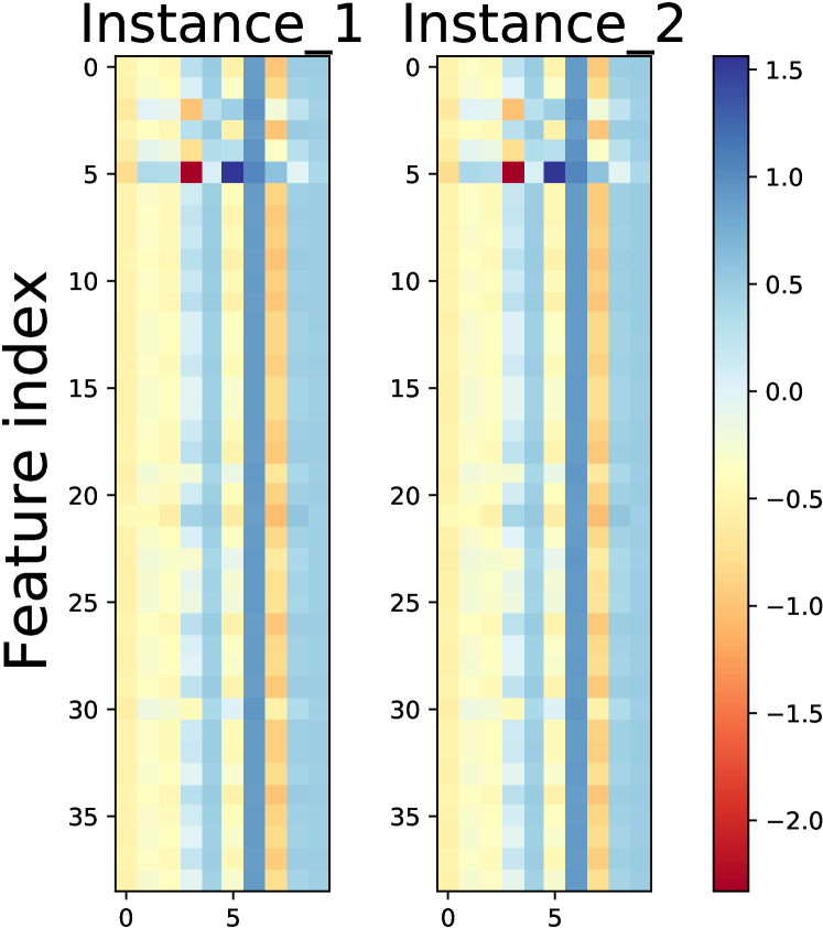
(a) Self-Attention

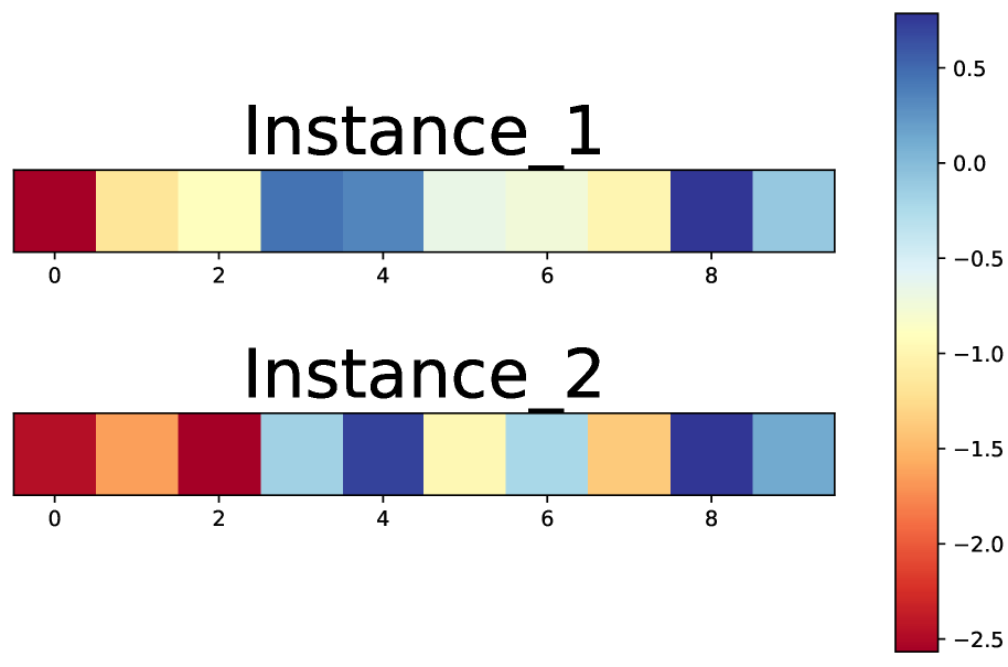
(b) CIE

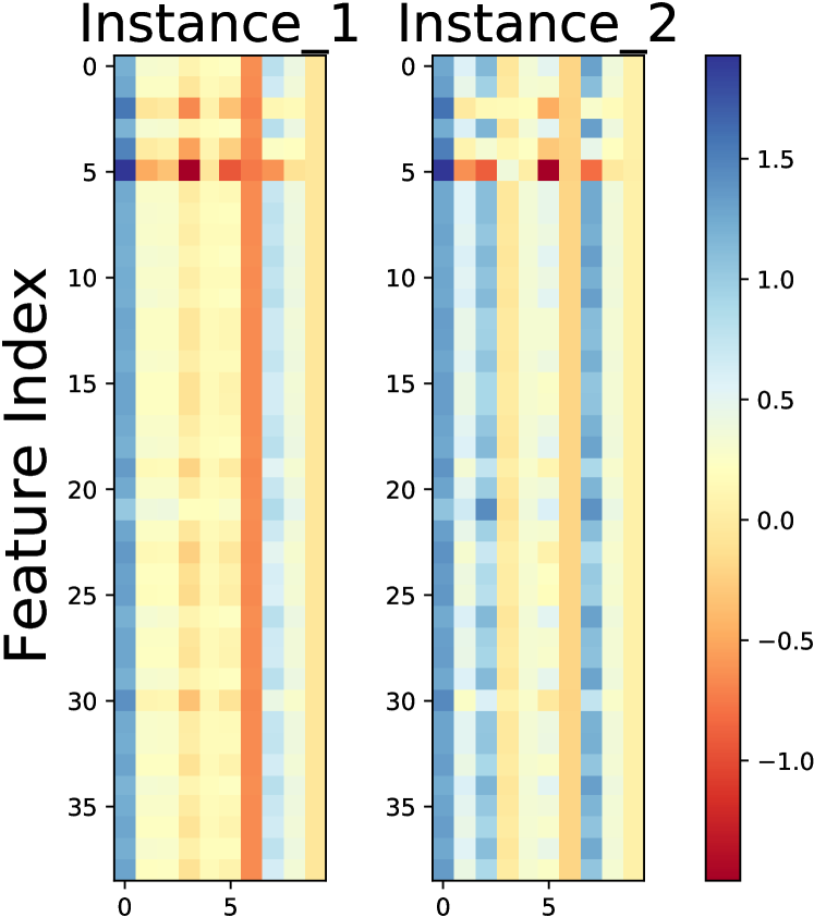
(c) IEU

Figure 8. Heatmap of features learned by IEU and its complements: Self-attention and CIE.

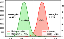
Figure 9. Distribution of bit-level weights in 100K instances.

6. Conclusion

In this paper, we propose a novel module named FRNet, which can learn context-aware feature representations and be used in most CTR prediction models to enhance their performance. In FRNet, we design IEU to integrate contextual information and cross-feature relationships, enabling self-attention to incorporate contextual information within each instance. We also design the CSGate to integrate the original and complementary features representations with learned bit-level weights. Detailed ablation study shows that each design of FRNet contributes to the overall performance. Furthermore, comprehensive experiments verify the effectiveness, efficiency, and compatibility of our proposed method.

- (1)
- Chen et al. (2021) Bo Chen, Yichao Wang, Zhirong Liu, Ruiming Tang, Wei Guo, Hongkun Zheng, Weiwei Yao, Muyu Zhang, and Xiuqiang He. 2021. Enhancing Explicit and Implicit Feature Interactions via Information Sharing for Parallel Deep CTR Models. In Proceedings of the 30th ACM International Conference on Information & Knowledge Management. 3757–3766.
- Cheng et al. (2016) Heng-Tze Cheng, Levent Koc, Jeremiah Harmsen, Tal Shaked, Tushar Chandra, Hrishi Aradhye, Glen Anderson, Greg Corrado, Wei Chai, Mustafa Ispir, et al. 2016. Wide & deep learning for recommender systems. In Proceedings of the 1st workshop on deep learning for recommender systems. 7–10.
- Cheng et al. (2020) Weiyu Cheng, Yanyan Shen, and Linpeng Huang. 2020. Adaptive factorization network: Learning adaptive-order feature interactions. In Proceedings of the AAAI Conference on Artificial Intelligence, Vol. 34. 3609–3616.
- Covington et al. (2016) Paul Covington, Jay Adams, and Emre Sargin. 2016. Deep neural networks for youtube recommendations. In Proceedings of the 10th ACM conference on recommender systems. 191–198.
- Gehring et al. (2017) Jonas Gehring, Michael Auli, David Grangier, Denis Yarats, and Yann N Dauphin. 2017. Convolutional sequence to sequence learning. In International Conference on Machine Learning. PMLR, 1243–1252.
- Guo et al. (2021) Huifeng Guo, Bo Chen, Ruiming Tang, Weinan Zhang, Zhenguo Li, and Xiuqiang He. 2021. An embedding learning framework for numerical features in ctr prediction. In Proceedings of the 27th ACM SIGKDD Conference on Knowledge Discovery & Data Mining. 2910–2918.
- Guo et al. (2017) Huifeng Guo, Ruiming Tang, Yunming Ye, Zhenguo Li, and Xiuqiang He. 2017. DeepFM: a factorization-machine based neural network for CTR prediction. In Proceedings of the 26th International Joint Conference on Artificial Intelligence. 1725–1731.
- He et al. (2015) Kaiming He, Xiangyu Zhang, Shaoqing Ren, and Jian Sun. 2015. Delving deep into rectifiers: Surpassing human-level performance on imagenet classification. In Proceedings of the IEEE international conference on computer vision. 1026–1034.
- He et al. (2016) Kaiming He, Xiangyu Zhang, Shaoqing Ren, and Jian Sun. 2016. Deep residual learning for image recognition. In Proceedings of the IEEE conference on computer vision and pattern recognition. 770–778.
- He and Chua (2017) Xiangnan He and Tat-Seng Chua. 2017. Neural factorization machines for sparse predictive analytics. In Proceedings of the 40th International ACM SIGIR conference on Research and Development in Information Retrieval. 355–364.
- He et al. (2014) Xinran He, Junfeng Pan, Ou Jin, Tianbing Xu, Bo Liu, Tao Xu, Yanxin Shi, Antoine Atallah, Ralf Herbrich, Stuart Bowers, et al. 2014. Practical lessons from predicting clicks on ads at facebook. In Proceedings of the Eighth International Workshop on Data Mining for Online Advertising. 1–9.
- Hu et al. (2018) Jie Hu, Li Shen, and Gang Sun. 2018. Squeeze-and-excitation networks. In Proceedings of the IEEE conference on computer vision and pattern recognition. 7132–7141.
- Huang et al. (2020) Tongwen Huang, Qingyun She, Zhiqiang Wang, and Junlin Zhang. 2020. GateNet: Gating-Enhanced Deep Network for Click-Through Rate Prediction. arXiv preprint arXiv:2007.03519 (2020).
- Huang et al. (2019) Tongwen Huang, Zhiqi Zhang, and Junlin Zhang. 2019. FiBiNET: combining feature importance and bilinear feature interaction for click-through rate prediction. In Proceedings of the 13th ACM Conference on Recommender Systems. 169–177.
- Juan et al. (2016) Yuchin Juan, Yong Zhuang, Wei-Sheng Chin, and Chih-Jen Lin. 2016. Field-aware factorization machines for CTR prediction. In Proceedings of the 10th ACM Conference on Recommender Systems. 43–50.
- Kingma and Ba (2015) Diederik P Kingma and Jimmy Ba. 2015. Adam: A Method for Stochastic Optimization. In ICLR (Poster).
- Li et al. (2020a) Zeyu Li, Wei Cheng, Yang Chen, Haifeng Chen, and Wei Wang. 2020a. Interpretable click-through rate prediction through hierarchical attention. In Proceedings of the 13th International Conference on Web Search and Data Mining. 313–321.
- Li et al. (2020b) Z Li, J Zhang, Y Gong, Y Yao, and Q Wu. 2020b. Field-wise Learning for Multi-field Categorical Data. In Conference on Neural Information Processing Systems.
- Lian et al. (2018) Jianxun Lian, Xiaohuan Zhou, Fuzheng Zhang, Zhongxia Chen, Xing Xie, and Guangzhong Sun. 2018. xdeepfm: Combining explicit and implicit feature interactions for recommender systems. In Proceedings of the 24th ACM SIGKDD International Conference on Knowledge Discovery & Data Mining. 1754–1763.
- Liu et al. (2019) Bin Liu, Ruiming Tang, Yingzhi Chen, Jinkai Yu, Huifeng Guo, and Yuzhou Zhang. 2019. Feature generation by convolutional neural network for click-through rate prediction. In The World Wide Web Conference. 1119–1129.
- Lu et al. (2020) Wantong Lu, Yantao Yu, Yongzhe Chang, Zhen Wang, Chenhui Li, and Bo Yuan. 2020. A Dual Input-aware Factorization Machine for CTR Prediction. In IJCAI. 3139–3145.
- Luo et al. (2020) Yuanfei Luo, Hao Zhou, Wei-Wei Tu, Yuqiang Chen, Wenyuan Dai, and Qiang Yang. 2020. Network On Network for Tabular Data Classification in Real-world Applications. In Proceedings of the 43rd International ACM SIGIR Conference on Research and Development in Information Retrieval. 2317–2326.
- Pan et al. (2018) Junwei Pan, Jian Xu, Alfonso Lobos Ruiz, Wenliang Zhao, Shengjun Pan, Yu Sun, and Quan Lu. 2018. Field-weighted factorization machines for click-through rate prediction in display advertising. In Proceedings of the 2018 World Wide Web Conference. 1349–1357.
- Pan et al. (2021) Yujie Pan, Jiangchao Yao, Bo Han, Kunyang Jia, Ya Zhang, and Hongxia Yang. 2021. Click-through Rate Prediction with Auto-Quantized Contrastive Learning. arXiv preprint arXiv:2109.13921 (2021).
- Qu et al. (2018) Yanru Qu, Bohui Fang, Weinan Zhang, Ruiming Tang, Minzhe Niu, Huifeng Guo, Yong Yu, and Xiuqiang He. 2018. Product-based neural networks for user response prediction over multi-field categorical data. ACM Transactions on Information Systems (TOIS) 37, 1 (2018), 1–35.
- Rendle (2012) Steffen Rendle. 2012. Factorization machines with libfm. ACM Transactions on Intelligent Systems and Technology (TIST) 3, 3 (2012), 1–22.
- Richardson et al. (2007) Matthew Richardson, Ewa Dominowska, and Robert Ragno. 2007. Predicting clicks: estimating the click-through rate for new ads. In Proceedings of the 16th international conference on World Wide Web. 521–530.
- Song et al. (2019) Weiping Song, Chence Shi, Zhiping Xiao, Zhijian Duan, Yewen Xu, Ming Zhang, and Jian Tang. 2019. Autoint: Automatic feature interaction learning via self-attentive neural networks. In Proceedings of the 28th ACM International Conference on Information and Knowledge Management. 1161–1170.
- Van der Maaten and Hinton (2008) Laurens Van der Maaten and Geoffrey Hinton. 2008. Visualizing data using t-SNE. Journal of machine learning research 9, 11 (2008).
- Vaswani et al. (2017) Ashish Vaswani, Noam Shazeer, Niki Parmar, Jakob Uszkoreit, Llion Jones, Aidan N Gomez, Łukasz Kaiser, and Illia Polosukhin. 2017. Attention is all you need. In Advances in neural information processing systems. 5998–6008.
- Wang et al. (2017) Ruoxi Wang, Bin Fu, Gang Fu, and Mingliang Wang. 2017. Deep & cross network for ad click predictions. In Proceedings of the ADKDD’17. 1–7.
- Wang et al. (2021b) Ruoxi Wang, Rakesh Shivanna, Derek Cheng, Sagar Jain, Dong Lin, Lichan Hong, and Ed Chi. 2021b. DCN V2: Improved Deep & Cross Network and Practical Lessons for Web-scale Learning to Rank Systems. In Proceedings of the Web Conference 2021. 1785–1797.
- Wang et al. (2021a) Zhiqiang Wang, Qingyun She, and Junlin Zhang. 2021a. MaskNet: Introducing Feature-Wise Multiplication to CTR Ranking Models by Instance-Guided Mask. arXiv preprint arXiv:2102.07619 (2021).
- Wei et al. (2021) Zhikun Wei, Xin Wang, and Wenwu Zhu. 2021. AutoIAS: Automatic Integrated Architecture Searcher for Click-Trough Rate Prediction. In Proceedings of the 30th ACM International Conference on Information & Knowledge Management. 2101–2110.
- Wu et al. (2020) Shu Wu, Feng Yu, Xueli Yu, Qiang Liu, Liang Wang, Tieniu Tan, Jie Shao, and Fan Huang. 2020. TFNet: Multi-Semantic Feature Interaction for CTR Prediction. In Proceedings of the 43rd International ACM SIGIR Conference on Research and Development in Information Retrieval. 1885–1888.
- Xiao et al. (2017) Jun Xiao, Hao Ye, Xiangnan He, Hanwang Zhang, Fei Wu, and Tat-Seng Chua. 2017. Attentional factorization machines: learning the weight of feature interactions via attention networks. In Proceedings of the 26th International Joint Conference on Artificial Intelligence. 3119–3125.
- Yang et al. (2020) Yi Yang, Baile Xu, Shaofeng Shen, Furao Shen, and Jian Zhao. 2020. Operation-aware Neural Networks for user response prediction. Neural Networks 121 (2020), 161–168.
- Yu et al. (2021) Runlong Yu, Yuyang Ye, Qi Liu, Zihan Wang, Chunfeng Yang, Yucheng Hu, and Enhong Chen. 2021. XCrossNet: Feature Structure-Oriented Learning for Click-Through Rate Prediction. In PAKDD (2). Springer, 436–447.
- Yu et al. (2019) Yantao Yu, Zhen Wang, and Bo Yuan. 2019. An Input-aware Factorization Machine for Sparse Prediction. In IJCAI. 1466–1472.
- Zhang et al. (2016) Weinan Zhang, Tianming Du, and Jun Wang. 2016. Deep learning over multi-field categorical data. In European conference on information retrieval. Springer, 45–57.
- Zhao et al. (2021b) Keke Zhao, Xing Zhao, Qi Cao, and Linjian Mo. 2021b. A Non-sequential Approach to Deep User Interest Model for Click-Through Rate Prediction. arXiv preprint arXiv:2104.06312 (2021).
- Zhao et al. (2020) Zihao Zhao, Zhiwei Fang, Yong Li, Changping Peng, Yongjun Bao, and Weipeng Yan. 2020. Dimension Relation Modeling for Click-Through Rate Prediction. In Proceedings of the 29th ACM International Conference on Information & Knowledge Management. 2333–2336.
- Zhao et al. (2021a) Zhishan Zhao, Sen Yang, Guohui Liu, Dawei Feng, and Kele Xu. 2021a. FINT: Field-aware INTeraction Neural Network For CTR Prediction. arXiv preprint arXiv:2107.01999 (2021).
- Zhou et al. (2018) Guorui Zhou, Xiaoqiang Zhu, Chenru Song, Ying Fan, Han Zhu, Xiao Ma, Yanghui Yan, Junqi Jin, Han Li, and Kun Gai. 2018. Deep interest network for click-through rate prediction. In Proceedings of the 24th ACM SIGKDD International Conference on Knowledge Discovery & Data Mining. 1059–1068.