Edge-enhanced Feature Distillation Network for Efficient Super-Resolution

Abstract

With the recently massive development in convolution neural networks, numerous lightweight CNN-based image super-resolution methods have been proposed for practical deployments on edge devices. However, most existing methods focus on one specific aspect: network or loss design, which leads to the difficulty of minimizing the model size. To address the issue, we conclude block devising, architecture searching, and loss design to obtain a more efficient SR structure. In this paper, we proposed an edge-enhanced feature distillation network, named EFDN, to preserve the high-frequency information under constrained resources. In detail, we build an edge-enhanced convolution block based on the existing reparameterization methods. Meanwhile, we propose edge-enhanced gradient loss to calibrate the reparameterized path training. Experimental results show that our edge-enhanced strategies preserve the edge and significantly improve the final restoration quality. Code is available at https://github.com/icandle/EFDN.

1 Introduction

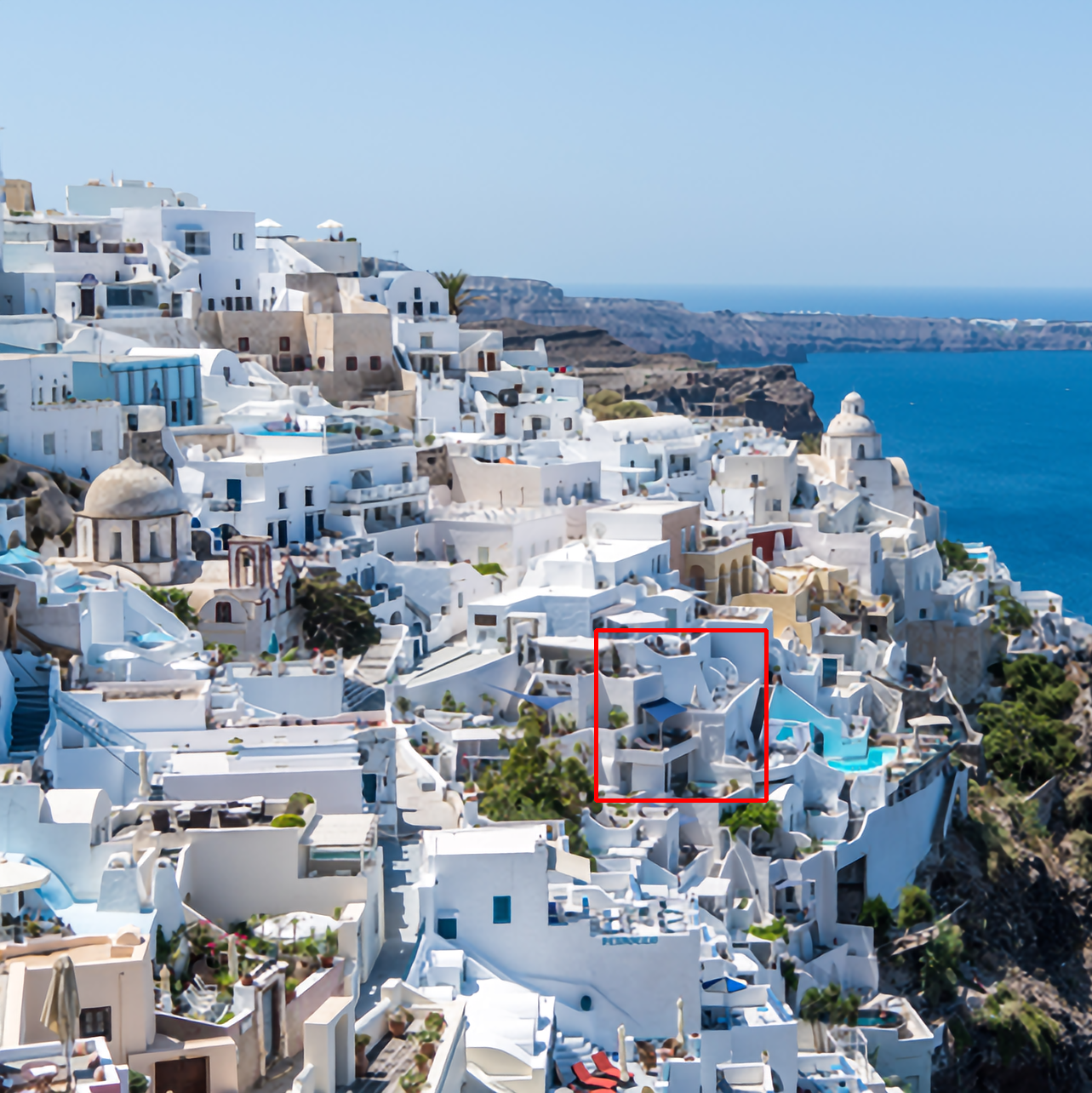
	HR
0823 from DIV2K	SR

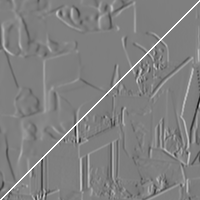
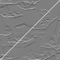
$\mathcal{L}_{x}=0.0201$	$\mathcal{L}_{y}=0.0092$	$\mathcal{L}_{l}=0.0015$

Figure 1: Visual results on DIV2K [2]. The lower right parts are ground truth gradient maps processed by the Sobel-(x,y) and Laplacian filters. The upper left part are results for EFDN.

Image super-resolution (SR) is a widely concerning low-level computer vision task that aims to build missing high-frequency information in degraded low-quality images. However, it is challenging to predict the appropriate images due to the ill-posed nature since one high-resolution (HR) image corresponds to plenty of low-resolution images. Many classical methods [36, 30, 31] have been proposed to address this problem, but their reconstruction quality under large magnification is often unsatisfactory. Recently, many convolution neural network (CNN) based approaches [9, 10, 16, 23, 38, 19, 26] were introduced to obtain realistic super-resolution images. Notwithstanding, most of them focus on improving restoration quality while involuntarily increasing the model scale, resulting in difficulty for mobile devices deployment. In this paper, we mainly concentrate on deploying SR models under resource-limited conditions.

In order to design a qualified lightweight neural network, researchers cut into this problem from the perspective of parameter reduction and calculation reduction. Sticking to reducing the size of convolution and features, FSRCNN [10] first employed the post upscaling module, which removed both calculations and parameters. For more significant parameter reduction, the recurrent learning is leveraged in many works, including DRCN [17] and DRRN [29]. However, these recursive approaches cost more computation resources due to their limited representation capability. For instance, 17.9T multiply-add operations (MAdds) are spent in DRCN and 6.8T in DRRN, which are unbearable for mobile devices. Therefore, the researchers have shifted the critical point of efficient SR to designing effective modules and dedicated networks.

To this end, networks [3, 15, 14] and blocks [37, 7, 6, 40] were proposed to improve efficiency. In RFDN [24], the shallow residual block and dedicated distillation procedure are introduced to achieve superior performance under constrained conditions. However, its parameters and operations are still unaffordable for part of edge devices due to the dense connections. Zhang et al. [37] utilized a plain network with a re-parameterizable convolution block to accomplish real-time application on commodity mobile devices. But they suffer from PSNR drop like other simple networks. In addition to these manually designed networks and blocks, many methods based on neural architecture search (NAS) [28, 33, 5] and model pruning [20, 21] are proposed to obtain more flexible and lightweight networks. DLSR [12] introduced a differentiable NAS method to find a more flexible typology based on RFDN, which designs cell-level and network-level with meager cost. Nevertheless, DLSR overuses depth-wise convolution, bringing a large amount of activation and memory consumption. Hence, there is still room for improvement in designing an efficient SR model.

In order to address the above issues, we propose an efficient Edge-enhanced Feature Distillation Network (EFDN), which combines block composing, architecture searching, and loss designing to obtain a trade-off between the performance and light-weighting. For block composing, we sum up the re-parameterization methods [37, 7, 6, 8] and design a more effective and complex edge-enhanced diverse branch block. In detail, we employ several reasonable re-parameterizable branches to enhance the structural information extraction, and then we integrate them into a vanilla convolution to maintain the inference performance. To ensure the effective optimization of parallel branches in EDBB, we design an edge-enhanced gradient-variance loss (EG) based on gradient-variance loss [1]. The proposed loss enforces minimizing the difference between the computed variance maps, which is helpful to restore sharper edges. As shown in Fig. 1, we present the gradient maps calculated by different filters and the corresponding EG loss. In addition, the NAS strategy of DLSR is adopted to search a robust backbone.

Overall, our main contributions can be summarized as follows:

1. We propose a plug-in edge-enhanced diverse branch block by revisiting existing re-parameterization technologies. The block can improve the SR performance without extra cost for inference.

2. We design a novel gradient-variance loss function for edge information preserve. The loss can work with the proposed EDBB to achieve higher restoration quality.

3. We include block composing, NAS, and loss design into our EFDN framework. And our model achieves a competitive performance while maintaining an extremely lightweight inference.

2 Related Work

2.1 Efficient image super-resolution

In recent years, convolutional neural networks (CNNs) have greatly promoted the development of low-level computer vision tasks [11]. In the super-resolution field, Dong et al. [9] proposed SRCNN, the earliest CNN-based work which outperforms the traditional methods. However, SRCNN adopts post-upscaling architecture and large convolution layers, which would result in reduced operating efficiency. To remove the unnecessary computational cost, the authors re-implemented the upscaling module by a deconvolution layer and moved it to the tail part in [10]. Since then, plenty of CNN-based SR networks[23, 38, 26, 39] has been introduced to improve the reconstruction results. Nevertheless, most approaches leverage hundreds of convolution layers and attention mechanisms for higher quality while ignoring the applications under restricted resources.

To develop the efficient super-resolution in edge devices, Ahn et al. [3] proposed CARN-M, a residual network with a cascading mechanism, which can reduce parameters and computations at the expense of quality reduction. Hui et al. proposed an information distillation network [15] to explicitly split the intermediate feature to distill and compress the local long and short-path features. Based on IDN, IMDN [14] is introduced with a more reasonable feature distillation mechanism and effective adaptive cropping strategy. Enlightened by revisiting these distillation mechanisms, Liu et al. [24] proposed a novel channel splitting strategy that utilizes the convolution layer to implement dimensional change. Furthermore, they devise shallow residual blocks to improve the construction performance while maintaining the parameter scale. With these improvements, they won first place in the AIM 2020 efficient super-resolution challenge [35].

2.2 Re-parameterization

Re-parameterization has become an effective technique for efficient neural network design. Lei et al. [6] proposed an asymmetric convolution block (ACB) to strengthen the vanilla convolution by merging three different convolutions. Then in the AIM 2020 [35], FIMDN adopted the block into the super-resolution field and outperformed IMDN with fewer parameters. RepVGG [8] first added identity mapping and 1$\times$1 convolution into the re-parameterizable structure family, and DBB [7] further enriched the family with sequential convolutions like expanding-and-squeezing convolution. Based on these works, Zhang et al. [37] proposed an edge-oriented convolution block (ECB) to improve the performance of the real-time SR network in mobile devices.

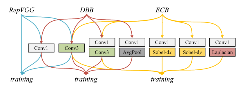
(a) Revisiting re-parameterizable typology.

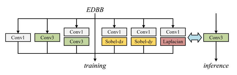
(b) Proposed edge-enhanced diverse branch block.

Figure 2: Illustration of re-parameterization method.

3 Proposed Method

3.1 Edge-enhanced diverse branch block

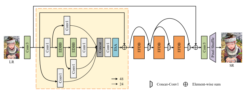
Figure 3: Network architecture of the proposed EFDN.

First, we revisit the existing re-parameterizable topology [8, 37, 7]. As shown in Fig. 2(a), we present the detail of RepVGG Block, DBB, and ECB. A total of eight different structures have been designed to improve the feature extraction ability of the vanilla convolution in different scenarios. Although the performance may be higher with more re-parameterizable branches, the expensive training cost is unaffordable for straightly integrating these paths. Meanwhile, another problem is that edge and structure information may be attenuated during the merging of parallel branches.

To address the above concerns, we build a more delicate and effective reparameterization block, namely Edge-enhanced Diverse Branch Block (EDBB), which can extract and preserve high-level structural information for the low-level task. As illustrated in Fig. 2(b), the EDBB consists of seven branches, summarized in following two categories.

Category I: a single convolution. A normal single convolution operator can be given as:

$$\sigma(\bm{x})=\bm{W}\ast\bm{x}+\bm{b},$$ (1)

Given the convolution operator ($\bm{W}$, $\bm{b}$) with a $h$$\times$$w$ kernel and the target convolution ($\bm{W}^{\rm I}$, $\bm{b}^{\rm I}$) with the kernel shape of $H$$\times$$W$ ($h\leq H$,$w\leq W$), the process of assigning reparameterized kernel from zero matrix can be given as:

$$\bm{W}^{\rm I}_{:,:,i+\lfloor\frac{H-h}{2}\rfloor,j+\lfloor\frac{W-w}{2}\rfloor} =\bm{W}_{:,:,i,j},$$ (2a)

$$\bm{b}^{\rm I} =\bm{b},$$ (2b)

While for shortcut operator, it can be treated as a special 1$\times$1 convolution, where $\bm{W}_{:,:,0,0}$ is an identity matrix.

Category II: sequential convolutions. Sequential convolutions are widely applied to further extract the hidden information from the feature maps. In the EDBB, we introduce expanding-and-squeezing convolution and scaled filter convolution to enhance the edge and structure signals. Generally, these re-parameterizable convolution sequences can be expressed by:

$$\sigma_{2}(\sigma_{1}(\bm{x}))=\bm{W}_{2}\ast(\bm{W}_{1}\ast\bm{x}+\bm{b}_{1})+\bm{b}_{2},$$ (3)

where the $\sigma_{1}$ is the first $D\times C\times 1\times 1$ convolution ($\bm{W}_{1}$, $\bm{b}_{1}$), and $\sigma_{2}$ is the second $C\times D\times K\times K$ convolution ($\bm{W}_{2}$, $\bm{b}_{2}$). To merge them into a $C\times C\times K\times K$ convolution ($\bm{W}^{\rm II}$, $\bm{b}^{\rm II}$), we transform the formula as the form of Eq. 1. According to [37, 7], we can obtain the target kernel in the following manner:

$$\bm{W}^{\rm II} =perm(\bm{W}_{1})\ast\bm{W}_{2},$$ (4a)

$$\bm{b}^{\rm II} =\bm{W}_{2}\ast rep(\bm{b}_{1})+\bm{b}_{2},$$ (4b)

where $perm$ and $rep$ are permuting and broadcasting operations to align weights correspondingly. For $\bm{W}_{1}$, the first two dimensions are exchanged to maintain the same size as $\bm{W}_{2}$. For $\bm{b}_{1}$, it is replicated to share the same shape as $\bm{b}_{2}$.

In the training stage, we train the model with EDBB to obtain more reasonable intermediate features. And then, we transfer EDBB into a vanilla convolution by calculating the sum of re-parameterized parameters. In general, the EDBB leads to quality promotion by utilizing more diverse re-parameterizable branches, and it maintains the running-time inference of vanilla convolution.

3.2 Network architecture

Following IMDN[14] and RFDN[24], we devise an edge-enhanced information distillation network (EFDN) to reconstruct high-quality SR images with sharp edges and clear structure under restricted resources. As illustrated in Fig. 3, our EFDN consists of a shallow feature extraction module, multiple edge-enhanced feature distillation blocks (EFDBs), and upscaling module. Specifically, we leverage a single vanilla convolution to generate the initial feature maps. Given the input LR image $I^{LR}$, this information extraction process can be encapsulated as:

$$F_{0}=E(I^{LR}),$$ (5)

where the $E$ denotes the feature extraction function by a 3$\times$3 convolution, and $F_{0}$ is the extracted feature maps. This coarse feature is then sent to stacked EFDBs for further information refining. In detail, we replace the shallow residual block in [24] with the proposed EDBB to construct our EFDB. Different from IMDN and RFDN utilizing dense distillation connections to process input features progressively, we adopt network-level NAS strategy proposed in DLSR [12] to decide the feature connection paths. The searched structure is shown in the orange dashed box. We denote the proposed EFDB as $H_{n}$, the information distillation procedure can be described as:

$$F_{1} =H_{1}(F_{0}),$$ (6)

$$F_{2} =H_{2}(F_{1}),$$

$$F_{3} =H_{3}(C_{1}(F_{1},F_{2})),$$

$$F_{4} =C_{3}(F_{2},H_{4}(C_{2}(F_{2},F_{3})))+F_{0},$$

where $C_{n}$ is $n$-th fusion operator consisting of concatenation and 1$\times$1 convolution. $F_{n}$ is the $n$-th output feature. Finally, the SR images are generated by upscaling module:

$$I^{SR}=R(F_{4}),$$ (7)

where $R$ consists of a 3$\times$3 convolution and sub-pixel operation to convert feature maps to images.

3.3 Edge-enhanced gradient-variance loss

In previous work[23], $\mathcal{L}_{1}$ and $\mathcal{L}_{2}$ loss have been in common usage to obtain higher evaluation indicators. The network trained with these loss functions often leads to the loss of structural information. Although the edge-oriented components are added to the EDBB, it is hard to ensure their effectiveness during the complex training procedure of seven parallel branches. Inspired by the gradient variance (GV) loss [1], we proposed an edge-enhanced gradient-variance (EG) loss, which utilizes the filters of the EDBB to monitor the optimization of the model. In detail, the HR image $I^{HR}$ and SR image $I^{SR}$ are transferred to gray-scale images $G^{HR}$ and $G^{SR}$. We leverage the Sobel and Laplacian filters to compute the gradient maps and then unfold gradient maps into $\frac{HW}{n^{2}}\times n^{2}$ patches $G_{x}$, $G_{y}$, $G_{l}$. The $i$-th variance maps can be formulated as:

$$v_{i}=\frac{\sum^{n^{2}}_{j=1}(G_{i,j}-\bar{G}_{i})^{2}}{n^{2}-1}$$ (8)

where $\bar{G}_{i}$ is the mean value of the $i$-th patch. Thus, we can calculate the variance metrics $v_{x}$,$v_{y}$,$v_{l}$ of HR and SR images, respectively. Referring to GV-loss, we can obtain the gradient variance loss of different filter by:

$$\mathcal{L}_{x} =\mathds{E}_{I^{SR}}\|v^{HR}_{x}-v^{SR}_{x}\|_{2}$$ (9)

$$\mathcal{L}_{y} =\mathds{E}_{I^{SR}}\|v^{HR}_{y}-v^{SR}_{y}\|_{2}$$

$$\mathcal{L}_{l} =\mathds{E}_{I^{SR}}\|v^{HR}_{l}-v^{SR}_{l}\|_{2}$$

Besides, we add $\mathcal{L}_{1}$ to accelerate convergence and improve the restoration performance. In order to better optimize the edge-oriented branches of EDBBs and preserve sharp edges for visual effects, we set trade-off coefficients $\lambda_{x}$, $\lambda_{y}$, and $\lambda_{l}$, which are related to the scaled parameters of corresponding branches. In detail, we replace the last convolution layer with EDBB during the pre-training process to obtain the reasonable scaled parameters $s_{x}$, $s_{y}$, and $s_{l}$ of different branches. Then, we determine the $\lambda$ by calculating the normalized weights of $s$, and we transfer the EDBB back into a vanilla convolution for more accessible training. The summative loss function can be expressed by:

$$\mathcal{L}_{EG}=\mathcal{L}_{1}+\lambda_{x}\mathcal{L}_{x}+\lambda_{y}\mathcal{L}_{y}+\lambda_{l}\mathcal{L}_{l}$$ (10)

4 Experiments

4.1 Datasets and metrics

In the training stage, we use DIV2K [2] and Flick2K [23] (DF2K) to train our models. A total of 3450 images are included to produce high-resolution and bicubic down-sampled image pairs. In the evaluation stage, we utilize four commonly used benchmark datasets: Set5 [4], Set14 [34], BSD100 [25], and Urban100[13]. In terms of evaluation metrics, peak signal-to-noise ratio (PSNR) and structural similarity (SSIM) [32] are calculated in the $Y$ channel of $YCbCr$ form to validate the quality of generated images.

4.2 Implementation details

To obtain the LR-HR images pairs, we leverage bicubic interpolation to downscale the 2K resolution images. We augment the training datasets by horizontal flips and $90^{\circ}$ rotations. The HR path size and mini-batch size are determined by the training step. The training procedure can be summarized as follows.

1. Pre-training the $\times$2 model on DIV2K. The LR patch size is set to 64$\times$64, and the mini-batch size is 64. $\mathcal{L}_{1}$ loss and Adam optimizer [18] are utilized in optimization. The initial learning rate is defined as $1\times 10^{-3}$. Referring to [40], we employ the cosine annealing learning scheme to accelerate convergence.

2. Training models on DF2K. In this step, The LR patch size is 64$\times$64, and the mini-batch size is 32. We use $\mathcal{L}_{EG}$ in Eq. 10 to provide a better visual effect. The initial learning rate is set to $5\times 10^{-4}$.

3. Fine-tuning on DF2K. The LR patch size and mini-batch size are 120$\times$120 and 32, respectively. The $\mathcal{L}_{2}$ loss is chosen to promote the PSNR value. The learning rate is initialized to $1\times 10^{-5}$.

4. Reparameterizing and fine-tuning on DIV2K. The LR patch size and mini-batch size are 160$\times$160 and 8, respectively. The $\mathcal{L}_{2}$ loss is used, and the learning rate starts from $1\times 10^{-6}$.

The proposed method is implemented under the PyTorch framework [27] with an NVIDIA RTX 3090 GPU.

4.3 Model analysis

In this subsection, we investigate model complexity including model size and running-time, and the effectiveness of EDBB and EG loss.

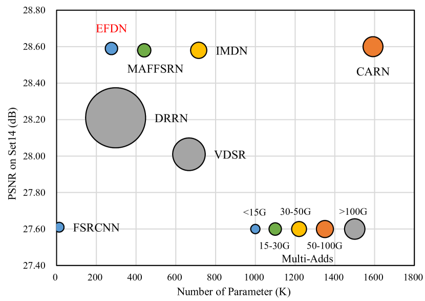
Figure 4: Trade-off between performance and model complexity on Set14 [34] $\times$4 dataset. The multi-adds operation is calculated with 320$\times$180 input.

Method	PSNR	Paras.	FLOPs	Act.	Mem.
IMDN [14]	29.13/28.78	893K	58.53	154.14	120
RFDN [24]	29.04/28.75	433K	27.10	112.03	200
PAN [40]	29.01/28.70	272K	32.19	270.53	311
EFDN (Ours)	29.00/28.66	276K	16.73	111.12	168

Table 1: Results on method complexity (number of parameters, FLOPs, GPU memory consumption, number of activations).

4.3.1 Model compexity

In Fig. 4, we provide an overview of our Network’s deployment performance. We can find that our EFDN obtains a better trade-off between the SR quality and model size. To evaluate the method complexity of our EFDN precisely, we compare several lightweight networks in Tab. 1. For fairness, the benchmark in AIM 2020 [35] is leveraged to evaluate the inference performance. The table shows that our EFDN achieves comparable PSNR on validation and test datasets while consuming fewer resources. In detail, only 16.73G FLOPs are spent during the reconstruction, which is about half of PAN [40] and 29% of IMDN [14]. Moreover, the EFDN also has the minimum activation operations and the second least parameters and memory-consuming among these models. In terms of running time, we compare our approach with IMDN on an NVIDIA RTX 3090 and an RTX 2070-maxQ to evaluate the efficiency in Tab. 2. Our EFDN is significantly faster than IMDN on different GPUs.

Method	Time on 2070-maxQ	Time on 3090
IMDN [14]	0.158s	0.092s
EFDN (Ours)	0.089s	0.019s

Table 2: Results on running-time.

Table 3: Ablation study of re-parameterizable typology and loss function on Set5 [4], Set14 [34], B100 [25], Urban100 [13] ($\times$2). We compare the our EDBB to existing blocks on FSRCNN and test different designs on VDSR. The overall improvement by EDBB and $\mathcal{L}_{EG}$ are valided in FSRCNN, VDSR, and *EFDN. The best/second-best results are highlighted and underlined. (FSRCNN and VDSR are re-implemented, and BN layers are discarded during experiments.)

	Block	3$\times$3 Conv	1$\times$1 Conv	Identity	Expand- Squeeze	Scaled Filter	Set5	Set14	B100	Urban100
FSRCNN [10]	Baseline-$\mathcal{L}_{1}$	✓					37.09/0.9569	32.75/0.9098	31.56/0.8913	30.00/0.9037
	Baseline-$\mathcal{L}_{EG}$	✓					37.14/0.9571	32.77/0.9103	31.58/0.8917	30.00/0.9040
	RepVGG [8]	✓	✓	✓			37.15/0.9571	32.78/0.9102	31.59/0.8916	30.06/0.9045
	DBB [7]	✓	✓		✓	Avgpool	37.18/0.9572	32.77/0.9103	31.60/0.8918	30.11/0.9050
	ECB [37]	✓			✓	Laplacian & Sobel	37.17/0.9572	32.80/0.9103	31.59/0.8915	30.09/0.9044
	EDBB-$\mathcal{L}_{1}$	✓	✓	✓	✓	Laplacian & Sobel	37.19/0.9573	32.80/0.9104	31.61/0.8919	30.14/0.9052
	EDBB-$\mathcal{L}_{EG}$	✓	✓	✓	✓	Laplacian & Sobel	37.27/0.9576	32.86/0.9109	31.65/0.8926	30.25/0.9069
VDSR [16]	Baseline-$\mathcal{L}_{1}$	✓					37.69/0.9593	33.24/0.9142	31.99/0.8970	31.30/0.9198
	Baseline-$\mathcal{L}_{EG}$	✓					37.72/0.9595	33.30/0.9147	32.02/0.8978	31.40/0.9215
	EDBB-$\mathcal{L}_{1}$	✓		✓	✓	Laplacian & Sobel	37.73/0.9594	33.26/0.9143	31.99/0.8968	31.32/0.9205
	EDBB-$\mathcal{L}_{1}$	✓	✓		✓	Laplacian & Sobel	37.73/0.9596	33.33/0.9145	32.02/0.8973	31.38/0.9205
	EDBB-$\mathcal{L}_{1}$	✓	✓	✓	✓	Avgpool	37.68/0.9593	33.28/0.9142	32.00/0.8971	31.27/0.9190
	EDBB-$\mathcal{L}_{1}$	✓	✓	✓	✓	Laplacian & Sobel	37.76/0.9595	33.33/0.9147	32.03/0.8975	31.41/0.9207
	EDBB-$\mathcal{L}_{EG}$	✓	✓	✓	✓	Laplacian & Sobel	37.85/0.9600	33.41/0.9158	32.10/0.8987	31.65/0.9237
*	Baseline-$\mathcal{L}_{1}$	✓					37.91/0.9601	33.44/0.9168	32.12/0.8990	31.82/0.9253
	EDBB-$\mathcal{L}_{EG}$	✓	✓	✓	✓	Laplacian & Sobel	38.00/0.9604	33.57/0.9179	32.18/0.8998	32.05/0.9275

Table 4: Average PSNR/SSIM for scale $\times$2 and $\times$4 on datasets Set5 [4], Set14 [34], B100 [25], Urban100 [13] with bicubic degradation. The parameters and multi-adds are calculated with 1280$\times$720 shape output.The best/second-best results are highlighted and underlined.

Dataset	Scale	Bicubic	FSRCNN [10]	VDSR [16]	IDN [15]	CARN [3]	IMDN [14]	PAN [40]	EFDN (Ours)
		Para/MAdds	12K/4.6G	665K/612.6G	553K/31.1G	1592K/90.9G	715K/41.0G	272K/28.2G	276K/14.7G
Set5	$\times$2	33.66/0.9299	37.00/0.9558	37.53/0.9587	37.83/0.9600	37.76/0.9590	38.00/0.9605	38.00/0.9605	38.00/0.9604
	$\times$4	28.42/0.8104	31.35/0.8838	31.82/0.8903	32.13/0.8937	32.21/0.8948	32.13/0.8948	32.13/0.8948	32.08/0.8931
Set14	$\times$2	30.24/0.8688	32.63/0.9088	33.03/0.9124	33.30/0.9148	33.52/0.9166	33.63/0.9177	33.59/0.9181	33.57/0.9179
	$\times$4	26.00/0.7027	27.61/0.7550	28.01/0.7674	28.25/0.7730	28.60/0.7806	28.58/0.7811	28.60/0.7822	28.58/0.7809
B100	$\times$2	29.56/0.8403	31.53/0.8920	31.90/0.8960	32.08/0.8985	32.09/0.8978	32.19/0.8996	32.18/0.8997	32.18/0.8998
	$\times$4	25.96/0.6675	26.98/0.7150	27.29/0.7251	27.41/0.7297	27.58/0.7349	27.56/0.7353	27.59/0.7363	27.56/0.7354
Urban100	$\times$2	26.88/0.8403	29.88/0.9020	30.76/0.9140	31.27/0.9196	31.92/0.9256	32.17/0.9283	32.01/0.9273	32.05/0.9275
	$\times$4	23.14/0.6577	24.62/0.7280	25.18/0.7524	25.41/0.7632	26.07/0.7837	26.04/0.7838	26.11/0.7854	26.00/0.7815

4.3.2 Ablation studies of EDBB and EG loss

To evaluate the effectiveness of the proposed EDBB, we first compare it to other re-parameterization approaches on FSRCNN [10] in Tab. 3. We can observe that all four blocks can improve the PSNR/SSIM values, while our EDBB leads to higher performance improvement (PSNR: +0.05$\thicksim$0.14dB, SSIM: +0.0004$\thicksim$0.0015 on FSRCNN). We also examine the EDBB on the deeper VDSR [16] framework by removing or replacing re-parameterizable components. The results in Tab. 3 suggest that any branch change may lead to a quality drop. Overall, we employ EDBB as the core feature extractor in the EFDN backbone to improve the SR performance.

Additionally, we assess the impact of loss functions on the final resolving quality. In detail, we leverage $\mathcal{L}_{1}$ and $\mathcal{L}_{EG}$ onto the baseline and EDBB model, respectively. As listed in Tab. 3, the baseline trained by $\mathcal{L}_{EG}$ brings a slight improvement on PSNR but a performance boost on SSIM. For instance, the PSNR and SSIM of Urban100 are developed by 0.03dB and 0.0008 on VDSR, respectively. For models equipping EDBB, the benefits of using EG-loss are more significant. The combination method of EDBB and $\mathcal{L}_{EG}$ surpasses baseline by a large margin with 0.2dB improvement on three frameworks. Specifically, PSNR/SSIM results of our EFDN increased by 0.23dB/0.002 on the Urban100 testset. Moreover, we can infer from the advance of the SSIM index that the proposed $\mathcal{L}_{EG}$ helps the structure reconstruction by introducing edge-enhanced filters to calibrate EDBB training.

4.4 Comparison with state-of-the-arts

	HR	Bicubic	SRCNN	FSRCNN
291000 from B100 [25]	VDSR	CARN	IMDN	EFDN (Ours)
	HR	Bicubic	SRCNN	FSRCNN
img_093 from Urban100[13]	VDSR	CARN	IMDN	EFDN (Ours)
	HR	Bicubic	SRCNN	FSRCNN
img_099 from Urban100 [13]	VDSR	CARN	IMDN	EFDN (Ours)

Figure 5: Qualitative results of lightweight SR models with an upscaling factor $\times$4.

We compare our EFDN with several state-of-the-arts lightweight SR methods [9, 10, 16, 3, 15, 14, 40] on $\times$2 and $\times$4 tasks in Tab. 4. We use PSNR/SSIM as well as the numbers of parameters and Multi-adds to show model efficiency. It can be found that our method achieves comparable performance to the IMDN and CARN while using fewer parameters and computations. Specifically, the parameter number of EFDN is only 17% of CARN, and 38% of IMDN. For $\times$4 task, the muti-adds operands used in our EFDN are far less than these methods, which is 14.7G, about 53% in PAN and 16% in CARN. In general, our EFDN is the most lightweight model to maintain the fidelity performance.

Apart from numerical results, we also show the visual comparison in Fig. 5. From the patch of 291000, we can observe that our EFDN achieves similar reconstruction results with these high consumption models. In img_093 and img_099 from Urban100 [13], EFDN surpasses other methods by better quality and less deformation on structural details such as shadows and windows.

4.5 Challenge results

We have participated in NTIRE 2022 Efficient Super-Resolution Challenge [22]. This competition aims to devise a practical SR method that can maintain the PSNR value of IMDN [14] on DIV2K [2] validation with less resource consumption. Among the final 35 valid submissions, our EFDN ranks 9th in the running time track, 5th in the model complexity track, and 7th in the overall performance track.

5 Conclusion

In this paper, we propose an edge-enhanced feature distillation network for lightweight and accurate super-resolution. We devise an edge-enhanced diverse branch block, which employs more effective re-parameterizable paths to achieve better extraction capability. Furthermore, we design an edge-enhancing loss to maximize the effectiveness of the EDBB. By introducing these strategies, the model size is significantly and steadily reduced while maintaining a commendable SR performance. Numerous experiments have shown the efficiency of the proposed strengthening approaches.

References

- [1] Lusine Abrahamyan, Anh Minh Truong, Wilfried Philips, and Nikos Deligiannis. Gradient variance loss for structure-enhanced image super-resolution. arXiv preprint arXiv:2202.00997, 2022.
- [2] Eirikur Agustsson and Radu Timofte. Ntire 2017 challenge on single image super-resolution: Dataset and study. In CVPRW, pages 126–135, Honolulu, HI, USA, 2017.
- [3] Namhyuk Ahn, Byungkon Kang, and Kyung-Ah Sohn. Fast, accurate, and lightweight super-resolution with cascading residual network. In ECCV, pages 252–268, 2018.
- [4] Marco Bevilacqua, Aline Roumy, Christine Guillemot, and Marie-Line Alberi-Morel. Low-complexity single-image super-resolution based on nonnegative neighbor embedding. In BMVC, pages 1–10, Surrey, UK, 2012.
- [5] Xiangxiang Chu, Bo Zhang, Hailong Ma, Ruijun Xu, and Qingyuan Li. Fast, accurate and lightweight super-resolution with neural architecture search. In ICPR, pages 59–64. IEEE, 2021.
- [6] Xiaohan Ding, Yuchen Guo, Guiguang Ding, and Jungong Han. Acnet: Strengthening the kernel skeletons for powerful cnn via asymmetric convolution blocks. In ICCV, pages 1911–1920, Seoul, Korea (South), 2019.
- [7] Xiaohan Ding, Xiangyu Zhang, Jungong Han, and Guiguang Ding. Diverse branch block: Building a convolution as an inception-like unit. In CVPR, pages 10886–10895, 2021.
- [8] Xiaohan Ding, Xiangyu Zhang, Ningning Ma, Jungong Han, Guiguang Ding, and Jian Sun. Repvgg: Making vgg-style convnets great again. In CVPR, pages 13733–13742, 2021.
- [9] Chao Dong, Chen Change Loy, Kaiming He, and Xiaoou Tang. Image super-resolution using deep convolutional networks. IEEE TPAMI, 38(2):295–307, 2016.
- [10] Chao Dong, Chen Change Loy, and Xiaoou Tang. Accelerating the super-resolution convolutional neural network. In ECCV, pages 391–407, Amsterdam, The Netherlands, 2016.
- [11] Kaiming He, Xiangyu Zhang, Shaoqing Ren, and Jian Sun. Deep residual learning for image recognition. In CVPR, pages 770–778, Las Vegas, NV, USA, 2016.
- [12] Han Huang, Li Shen, Chaoyang He, Weisheng Dong, Haozhi Huang, and Guangming Shi. Lightweight image super-resolution with hierarchical and differentiable neural architecture search. arXiv preprint arXiv:2105.03939, 2021.
- [13] Jia-Bin Huang, Abhishek Singh, and Narendra Ahuja. Single image super-resolution from transformed self-exemplars. In CVPR, pages 5197–5206, Boston, MA, USA, 2015.
- [14] Zheng Hui, Xinbo Gao, Yunchu Yang, and Xiumei Wang. Lightweight image super-resolution with information multi-distillation network. In ACM MM, pages 2024–2032, Nice, France, 2019.
- [15] Zheng Hui, Xiumei Wang, and Xinbo Gao. Fast and accurate single image super-resolution via information distillation network. In CVPR, pages 723–731, 2018.
- [16] Jiwon Kim, Jung Kwon Lee, and Kyoung Mu Lee. Accurate image super-resolution using very deep convolutional networks. In CVPR, pages 1646–1654, Las Vegas, NV, USA, 2016.
- [17] Jiwon Kim, Jung Kwon Lee, and Kyoung Mu Lee. Deeply-recursive convolutional network for image super-resolution. In CVPR, pages 1637–1645, Las Vegas, NV, USA, 2016.
- [18] Diederik P. Kingma and Jimmy Ba. Adam: A method for stochastic optimization. In ICLR, San Diego, CA, USA, 2015.
- [19] Yawei Li, Shuhang Gu, Luc Van Gool, and Radu Timofte. Learning filter basis for convolutional neural network compression. In ICCV, 2019.
- [20] Yawei Li, Shuhang Gu, Kai Zhang, Luc Van Gool, and Radu Timofte. Dhp: Differentiable meta pruning via hypernetworks. In ECCV, pages 608–624. Springer, 2020.
- [21] Yawei Li, Wen Li, Martin Danelljan, Kai Zhang, Shuhang Gu, Luc Van Gool, and Radu Timofte. The heterogeneity hypothesis: Finding layer-wise differentiated network architectures. In CVPR, pages 2144–2153, 2021.
- [22] Yawei Li, Kai Zhang, Luc Van Gool, Radu Timofte, et al. Ntire 2022 challenge on efficient super-resolution: Methods and results. In CVPRW, 2022.
- [23] Bee Lim, Sanghyun Son, Heewon Kim, Seungjun Nah, and Kyoung Mu Lee. Enhanced deep residual networks for single image super-resolution. In CVPRW, pages 136–144, 2017.
- [24] Jie Liu, Jie Tang, and Gangshan Wu. Residual feature distillation network for lightweight image super-resolution. In ECCVW, volume 12537 of Lecture Notes in Computer Science, pages 41–55, Glasgow, UK, 2020. Springer.
- [25] David Martin, Charless Fowlkes, Doron Tal, and Jitendra Malik. A database of human segmented natural images and its application to evaluating segmentation algorithms and measuring ecological statistics. In ICCV, volume 2, pages 416–423, Vancouver, British Columbia, Canada, 2001.
- [26] Ben Niu, Weilei Wen, Wenqi Ren, Xiangde Zhang, Lianping Yang, Shuzhen Wang, Kaihao Zhang, Xiaochun Cao, and Haifeng Shen. Single image super-resolution via a holistic attention network. In ECCV, pages 191–207, Glasgow, UK, 2020.
- [27] Adam Paszke, Sam Gross, Francisco Massa, Adam Lerer, James Bradbury, Gregory Chanan, Trevor Killeen, Zeming Lin, Natalia Gimelshein, Luca Antiga, et al. Pytorch: An imperative style, high-performance deep learning library. Advances in neural information processing systems, 32, 2019.
- [28] Dehua Song, Chang Xu, Xu Jia, Yiyi Chen, Chunjing Xu, and Yunhe Wang. Efficient residual dense block search for image super-resolution. In AAAI, volume 34, pages 12007–12014, 2020.
- [29] Ying Tai, Jian Yang, and Xiaoming Liu. Image super-resolution via deep recursive residual network. In CVPR, pages 3147–3155, 2017.
- [30] Radu Timofte, Vincent De Smet, and Luc Van Gool. Anchored neighborhood regression for fast example-based super-resolution. In ICCV, pages 1920–1927, 2013.
- [31] Radu Timofte, Vincent De Smet, and Luc Van Gool. A+: Adjusted anchored neighborhood regression for fast super-resolution. In ACCV, pages 111–126. Springer, 2014.
- [32] Zhou Wang, Alan C Bovik, Hamid R Sheikh, and Eero P Simoncelli. Image quality assessment: from error visibility to structural similarity. IEEE TIP, 13(4):600–612, 2004.
- [33] Yan Wu, Zhiwu Huang, Suryansh Kumar, Rhea Sanjay Sukthanker, Radu Timofte, and Luc Van Gool. Trilevel neural architecture search for efficient single image super-resolution. arXiv preprint arXiv:2101.06658, 2021.
- [34] Roman Zeyde, Michael Elad, and Matan Protter. On single image scale-up using sparse-representations. In 7th International Conference on Curves and Surfaces, volume 6920, pages 711–730, Avignon, France, 2010.
- [35] Kai Zhang, Martin Danelljan, Yawei Li, Radu Timofte, Jie Liu, Jie Tang, Gangshan Wu, Yu Zhu, Xiangyu He, Wenjie Xu, et al. Aim 2020 challenge on efficient super-resolution: Methods and results. In ECCVW, pages 5–40. Springer, 2020.
- [36] Lei Zhang and Xiaolin Wu. An edge-guided image interpolation algorithm via directional filtering and data fusion. IEEE TIP, 15(8):2226–2238, 2006.
- [37] Xindong Zhang, Hui Zeng, and Lei Zhang. Edge-oriented convolution block for real-time super resolution on mobile devices. In ACM MM, pages 4034–4043, 2021.
- [38] Yulun Zhang, Kunpeng Li, Kai Li, Lichen Wang, Bineng Zhong, and Yun Fu. Image super-resolution using very deep residual channel attention networks. In ECCV, pages 286–301, Munich, Germany, 2018.
- [39] Yulun Zhang, Yapeng Tian, Yu Kong, Bineng Zhong, and Yun Fu. Residual dense network for image super-resolution. In CVPR, pages 2472–2481, Salt Lake City, UT, USA, 2018.
- [40] Hengyuan Zhao, Xiangtao Kong, Jingwen He, Yu Qiao, and Chao Dong. Efficient image super-resolution using pixel attention. In ECCVW, pages 56–72. Springer, 2020.