Expert-Calibrated Learning for Online Optimization with Switching Costs

Abstract.

We study online convex optimization with switching costs, a practically important but also extremely challenging problem due to the lack of complete offline information. By tapping into the power of machine learning (ML) based optimizers, ML-augmented online algorithms (also referred to as expert calibration in this paper) have been emerging as state of the art, with provable worst-case performance guarantees. Nonetheless, by using the standard practice of training an ML model as a standalone optimizer and plugging it into an ML-augmented algorithm, the average cost performance can be highly unsatisfactory. In order to address the “how to learn” challenge, we propose EC-L2O (expert-calibrated learning to optimize), which trains an ML-based optimizer by explicitly taking into account the downstream expert calibrator. To accomplish this, we propose a new differentiable expert calibrator that generalizes regularized online balanced descent and offers a provably better competitive ratio than pure ML predictions when the prediction error is large. For training, our loss function is a weighted sum of two different losses — one minimizing the average ML prediction error for better robustness, and the other one minimizing the post-calibration average cost. We also provide theoretical analysis for EC-L2O, highlighting that expert calibration can be even beneficial for the average cost performance and that the high-percentile tail ratio of the cost achieved by EC-L2O to that of the offline optimal oracle (i.e., tail cost ratio) can be bounded. Finally, we test EC-L2O by running simulations for sustainable datacenter demand response. Our results demonstrate that EC-L2O can empirically achieve a lower average cost as well as a lower competitive ratio than the existing baseline algorithms.

1. Introduction

Many real-world problems, such as energy scheduling in smart grids, resource management in clouds and rate adaptation in video streaming (Lin et al., 2011; Shi et al., 2020; Chen et al., 2018; Antoniadis et al., 2020; Li and Li, 2020), can be formulated as online convex optimization where an agent makes actions online based on sequentially revealed information. The goal of the agent is to minimize the sum of convex costs over an episode of multiple time steps. In addition, another crucial concern is that changing actions too abruptly is highly undesired in most practical applications. For example, frequently turning on and off servers in data centers can decrease the server lifespan and even create dangerous situations such as high inrush current (Malla et al., 2020), and a robot cannot arbitrarily change its position due to velocity constraints in navigation tasks (Shi et al., 2008). Consequently, such action impedance has motivated an emerging area of online convex optimization with switching costs, where the switching cost measures the degree of action changes across two consecutive time steps and acts a regularizer to make the online actions smoother.

While both empirically and theoretically important, online convex optimization with switching costs is extremely challenging. The key reason is that the optimal actions at different time steps are highly dependent on each other and hence require the complete offline future information, which is nonetheless lacking in practice (Chen et al., 2016; Rutten and Mukherjee, 2022).

To address the lack of offline future information (i.e., future cost functions or parameters), the set of algorithms that make actions only using online information have been quickly expanding. For example, some prior studies have considered online gradient descent (OGD) (Zinkevich, 2003; Comden et al., 2019), online balanced descent (OBD) (Chen et al., 2018), and regularized OBD (R-OBD) (Goel et al., 2019). Additionally, some other studies have also incorporated machine learning (ML) prediction of future cost parameters into the algorithm design under various settings. Notable examples include receding horizon control (RHC) (Comden et al., 2019) committed horizon control (CHC) (Chen et al., 2016), receding horizon gradient descent (RHGD) (Li et al., 2020) and adaptive balanced capacity scaling (ABCS) (Rutten and Mukherjee, 2022). Typically, these algorithms are developed based on classic optimization frameworks and offer guaranteed performance robustness in terms of the competitive ratio, which measures the worst-case ratio of the cost achieved by an online algorithm to the offline oracle’s cost. Nonetheless, despite the theoretical guarantee, a bounded worst-case competitive ratio does not necessarily translate into decreased average cost in most typical cases.

By exploiting the abundant historical data available in many practical applications (e.g., server management data center and energy scheduling in smart grids), the power of ML can go much further beyond simply predicting the future cost parameters. Indeed, state-of-the-art learning-to-optimize (L2O) techniques can even substitute conventional optimizers and directly predict online actions (Bengio et al., 2021; Chen et al., 2017; Kong et al., 2019). Thus, although it still remains under-explored in the context of online convex optimization with switching costs, the idea of using statistical ML to discover the otherwise hidden mapping from online information to actions is very natural and promising.

While ML-based optimizers can often result in a low average cost in typical cases, its drawback is also significant — lack of performance robustness. Crucially, albeit rare, some input instances can be arbitrarily “bad” for a pre-trained ML-based optimizer and empirically result in a high competitive ratio. This is a fundamental limitation of any statistical ML models, and can be attributed to several factors, including certain testing inputs drawn from a very different distribution than the training distribution, inadequate ML model capacity, ill-trained ML model weights, among others.

To provide worst-case performance guarantees and potentially leverage the advantage of an ML-based optimizer, ML-augmented algorithm designs have been recently considered in the context of online convex optimization with switching costs (Antoniadis et al., 2020; Rutten et al., 2022; Christianson et al., 2022). These algorithms often take a simplified view of the ML-based optimizer — the actions can come from any exogenous source, and an ML-based optimizer is just one of the possible sources. Concretely, the exogenous actions (viewed as ML predictions) are fed into another algorithm and modified following an expert-designed rule. We refer to this process as expert calibration. Thus, instead of using the original un-calibrated ML predictions, the agent adopts new expert-calibrated actions. Such expert calibration is inevitably crucial to achieve otherwise impossible performance robustness in terms of the competitive ratio, thus addressing the fundamental limitation of ML-based optimizers. But, unfortunately, a loose (albeit finite) upper bound on the competitive ratio in and of itself does not always lead to a satisfactory average cost performance. A key reason is that the standard practice is to train the ML-optimizer as a standalone optimizer that can give good actions on its own in many typical cases, but the the already-good actions in these cases will still be subsequently altered by expert calibration and hence lead to an increased average cost.

In this paper, we study online convex optimization with switching costs and propose EC-L2O (Expert-Calibrated Learning to Optimize), a novel expert-calibrated ML-based optimizer that minimizes the average cost while provably improving performance robustness compared to pure ML predictions. Concretely, based on a recurrent structure illustrated in Fig. 1, EC-L2O integrates a differentiable expert calibrator as a new downstream implicit layer following the ML-based optimizer. The expert calibrator generalizes state-of-the-art R-OBD (Goel et al., 2019) by adding a regularizer to keep R-OBD’s actions close to ML predictions. At each time step, the ML-based optimizer takes online information as its input and predicts an action, which is then calibrated by the expert algorithm. Importantly, we view the combination of the ML-based optimizer and the expert calibrator as an integrated entity, and holistically train the ML model to minimize the average post-calibration cost.

Compared to the standard practice of training a standalone ML model independently to minimize the average pre-calibration cost, the ML-based optimizer in EC-L2O is fully aware of the downstream expert calibrator, thus effectively mitigating the undesired average cost increase induced by expert calibration. Moreover, the inclusion of a differentiable expert calibrator allows us to leverage backpropagation to efficiently train the ML model, and also substantially improves the performance robustness compared to a standalone ML-based optimizer.

We rigorously prove that when the ML prediction errors are large, expert-calibrated ML predictions are guaranteed to improve the competitive ratio compared to pre-calibration predictions. On the other hand, when the predictions are of a good quality, the expert-calibrated ML predictions can lower the optimal competitive ratio achieved by standard R-OBD without predictions. Interestingly, with proper settings, the expert-calibrated ML predictins can achieve a sublinear cost regret compared to the ($L$-constrained) optimal oracle’s actions. We also provide the average cost bound, highlighting that expert calibration can benefit ML predictions when the training-testing distribution discrepancy is large. Additionally, we provide a bound on the high-percentile tail ratio of the cost achieved by EC-L2O to that of the offline optimal oracle (i.e., tail cost ratio). Our analysis demonstrates that EC-L2O can achieve both a low average cost and a bounded tail cost ratio by training the ML-based optimizer in EC-L2O over a weighted sum of two different losses — one for the pre-calibration ML predictions to have a low average prediction error, and the other one for the post-calibration

Finally, we test EC-L2O by running simulations for the application of sustainable datacenter demand response. Under a practical setting with training-testing distributional discrepancy, our results demonstrate that EC-L2O can achieve a lower average cost than expert algorithms as well as the pure ML-based optimizer. More interestingly, EC-L2O also achieves an empirically lower competitive ratio than the existing expert algorithms, resulting in the best average cost vs. competitive ratio tradeoff. This nontrivial result is due in great part to the differentiable expert calibrator and the loss function that we choose — both the average cost and ML prediction errors (which affect the competitive ratio) are taken into account in the training process.

To sum up, EC-L2O is the first to address the “how to learn” challenge for online convex optimization with switching costs. By integrating a differentiable expert calibrator and training the ML-based optimizer on a carefully designed loss function, EC-L2O minimizes the average cost, provably improves the performance robustness (compared to pure ML predictions), and offers probabilistic guarantee on the high-percentile tail cost ratio.

2. Problem Formulation

In general online optimization problems (Orabona, 2019), actions are made online according to sequentially revealed information to minimize the sum of the costs for an episode with a length of $T$ steps. Moreover, smooth actions are desired in many practical problems, such as dynamic server on/off provisioning in data centers and robot movement. Thus, we consider that changing actions across two consecutive steps also induces an additional cost referred to as switching cost, which acts as a regularizer and tends to make the online actions smoother over time.

More concretely, at the beginning of each step $t=1,\cdots,T$, the online information (a.k.a. context) $y_{t}\in\mathcal{Y}_{t}\subseteq\mathcal{R}^{q}$ is revealed to the agent, which then decides an action $x_{t}$ from an action set $\mathcal{X}\subseteq\mathcal{R}^{d}$. With action $x_{t}$, the agent incurs a hitting (or operational) cost $f(x_{t},y_{t})$, which is parameterized by the context $y_{t}$ and convex with respect to $x_{t}$, plus an additional switching cost $c(x_{t},x_{t-1})$ measuring how large the action change is. The goal of the agent is to minimize the sum of the hitting costs and the switching costs over an episode of $T$ steps as follows:

(1) $$\min_{x_{1},\cdots x_{T}}\sum_{t=1}^{T}f(x_{t},y_{t})+c(x_{t},x_{t-1}),$$

where the initial action $x_{0}$ is provided as an additional input to the agent prior to its first online action. The complete offline information is thus denoted as $\bm{s}=\left(x_{0},\bm{y}\right)\in\mathcal{S}$ with $\bm{y}=\left[y_{1},\cdots,y_{T}\right]$ and $\mathcal{S}=\mathcal{X}\times\prod_{t=1}^{T}\mathcal{Y}_{t}$. While we can formulate it as an equivalent hard constraint, our inclusion of the switching cost as a soft regularizer is well consistent with the existing literature (Shi et al., 2020; Lin et al., 2020; Chen et al., 2018).

The key challenge of solving Eqn. (1) comes from the action entanglement due to the switching cost: the complete contextual information $\bm{s}=\left(x_{0},\bm{y}\right)$ is required to make optimal actions, but it is lacking in advance and only sequentially revealed to the agent online.

Assumptions. We assume that the hitting cost function $f(x_{t},y_{t})$ is non-negative and $m$-strongly convex in $x_{t}$, which has also been considered in prior studies (Goel and Wierman, 2019; Goel et al., 2019). In addition, the switching cost $c(x_{t},x_{t-1})$ is measured in terms of the squared Mahalanobis distance with respect to a symmetric and positive-definite matrix $Q\in\mathcal{R}^{d\times d}$, i.e. $c(x_{t},x_{t-1})=\left(x_{t}-x_{t-1}\right)^{\top}Q\left(x_{t}-x_{t-1}\right)$ (De Maesschalck et al., 2000). Here, we assume that the smallest eigenvalue of $Q$ is $\frac{\alpha}{2}>0$ and the largest eigenvalue of $Q$ is $\frac{\beta}{2}$, which means $\frac{\alpha}{2}\|x_{t}-x_{t-1}\|^{2}\leq c(x_{t},x_{t-1})\leq\frac{\beta}{2}\|x_{t}-x_{t-1}\|^{2}$. The interpretation is that the switching cost quantifies the impedance of action movements in a linearly transformed space. For example, a diagonal matrix $Q$ with different non-negative diagonal elements can model the practical consideration that the change of a multi-dimensional action along certain dimensions can incur a larger cost than others (e.g., it might be easier for a flying drone to move horizontally than vertically). In the special case of $Q$ being an identity matrix, the switching cost reduces to the quadratic cost considered in (Goel and Wierman, 2019).

Performance metrics. For an online algorithm $\pi$, we denote its total cost, including hitting and switching costs, for a problem instance with context $\bm{s}=(x_{0},\bm{y})$ as $\mathrm{cost}(\pi,\bm{s})=\sum_{t=1}^{T}f(x_{t},y_{t})+c(x_{t},x_{t-1})$ where $x_{t}$, $t=1,\cdots,T$, are the actions produced by the algorithm $\pi$. Likewise, by denoting $\pi^{*}$ as the offline optimal oracle that has access to the complete information $\bm{s}=(x_{0},\bm{y})$ in advance and selects actions $x_{t}^{*}$, $t=1,\cdots,T$, we write the offline optimal cost as $\mathrm{cost}(\pi^{*},\bm{s})=\sum_{t=1}^{T}f(x^{*}_{t},y_{t})+c(x^{*}_{t},x^{*}_{t-1})$ with $x^{*}_{0}=x_{0}$.

The contextual information $\bm{s}=(x_{0},\bm{y})\in\mathcal{S}$ is drawn from an exogenous joint distribution $\mathbb{P}$. To evaluate the performance of $\pi$, we focus on two most important metrics — average cost and competitive ratio — defined as follows.

Definition 0 (Average cost).

For contextual information $\bm{s}=(x_{0},\bm{y})\sim\mathbb{P}$, the average cost of an algorithm $\pi$ over the joint distribution $\mathbb{P}$ is defined as

(2) $$\mathrm{AVG}(\pi)=\mathbb{E}\left[\mathrm{cost}(\pi,\bm{s})\right].$$

Definition 0 (Competitive ratio).

The competitive ratio of an algorithm $\pi$ is defined as

(3) $$\mathrm{CR}(\pi)=\sup_{\bm{s}\in\mathcal{S}}\frac{\mathrm{cost}(\pi,\bm{s})}{\mathrm{cost}(\pi^{*},\bm{s})}.$$

The average cost measures the expected performance in typical cases that an algorithm can attain given an environment distribution. On the other hand, the competitive ratio measures the worst-case performance of an algorithm relative to the offline optimal cost for any feasible problem instance that might be presented by the environment. While the average cost is important in practice, the conservative metric of competitive ratio quantifies the level of robustness of an algorithm. Importantly, the two metrics are different from each other: a lower average cost does not necessarily mean a lower competitive ratio, and vice versa.

Similar to the worst-case competitive ratio, we also consider the high-percentile tail ratio of the cost achieved by an online algorithm to that of the offline optimal oracle (Section 5.2). This metric, simply referred to as the tail cost ratio, provides a probabilistic view of the performance robustness of an algorithm.

3. A Simple ML-Based Optimizer

As a warm-up, we present a simple ML-based optimizer that is trained as a standalone model to produce good actions on its own. We emphasize that, while the ML-based optimizer can result in a low average cost, it has significant limitations in terms of the worst-case performance robustness.

3.1. Learning a Standalone Optimizer

Due to the agent’s lack of complete contextual information $\bm{s}=(x_{0},\bm{y})$ in advance, the crux of online convex optimization with switching costs is how to map the online information to an appropriate action so as to minimize the cost. Fortunately, most practical applications (e.g., server management data center and energy scheduling in smart grids) have abundant historical data available. This can be exploited by state-of-the-art ML techniques (e.g., L2O (Bengio et al., 2021; Chen et al., 2017)) and hence lead to the natural but still under-explored idea of using statistical ML to discover the otherwise difficult mapping from online contextual information to actions.

More concretely, following the state-of-the-art L2O techniques, we can first train a standalone ML-based optimizer $h_{W}$ parameterized by the model weight $W$, over a training dataset of historical and/or synthetic problem instances. For example, because of the universal approximation capability, we can employ a deep neural network (DNN) with recurrent structures as the underlying ML model $h_{W}$, where the recurrence accounts for the online optimization process. With online contextual information $y_{t}$ and the previous action $\tilde{x}_{t-1}$ as input, the ML-based optimizer with output $\tilde{x}_{t}$ can be trained to imitate the action $x^{\pi}_{t}$ of an expert (online) algorithm $\pi$ with good average or worst-case cost performance. Towards this end, the imitation loss defined in terms of the distance between the expert action and learnt action can be used as the loss function in the training process. Alternatively, we can also directly use the total cost over an entire episode as the loss function to supervise offline training of the ML-based optimizer (Bengio et al., 2021).

Given an unseen testing problem instance for inference, at each step, the pre-trained ML-based optimizer takes online contextual information and the previous action as its input, and predicts the current action as its output. Without causing ambiguity, we simply use ML predictions to represent the actions produced by the ML-based optimizer.

3.2. Limitations

With a large training dataset, the standalone ML-based optimizer can exploit the power of statistical learning and achieve a low cost on average, especially when the testing input distribution is well consistent with the training distribution (i.e., in-distribution testing). But, regardless of in-distribution or out-of-distribution testing, an ML-based optimizer can perform very poorly for some “bad” problem instances and empirically result in a high competitive ratio. This is a fundamental limitation of any statistical ML models, be they advanced DNNs or simple linear models.

The lack of performance robustness in these rare cases can be attributed to several factors, including certain testing inputs drawn from a very different distribution than the training distribution, inadequate ML model capacity, ill-trained ML model weights, among others. For example, even though the ML-based optimizer can perfectly imitate an expert’s action or obtain optimal actions for all the training problem instances, there is no guarantee that it can perform equally well for all testing problem instances due to the ML model capacity, inevitable generalization error as well as other factors.

While distributionally robust learning can alleviate the problem of testing distributional shifts relative to the training distribution (Kirschner et al., 2020; Zhang et al., 2021b), it still targets the average case (albeit over a wider distribution of testing problem instances) without addressing the worst-case performance, let alone its significantly increased training complexity.

To further quantify the lack of performance robustness, we define $\rho$-accurate prediction for the ML-based optimizer $h_{W}$ as follows.

Definition 0 ($\rho$-accurate Prediction).

Assume that for an input instance $\bm{s}=(x_{0},\bm{y})$, the offline-optimal oracle $\pi^{*}$ gives $x_{1}^{*},\cdots x_{T}^{*}$, and the offline optimal cost is $\mathrm{cost}(\pi^{*},\bm{s})=\sum_{t=1}^{T}f(x^{*}_{t},y_{t})+c(x^{*}_{t},x^{*}_{t-1})$. The predicted actions from the ML-based optimizer $h_{W}$, denoted as $\tilde{x}_{1},\cdots\tilde{x}_{T}$, are said to be $\rho$-accurate when the following is satisfied:

(4) $$\sum_{t=1}^{T}||\tilde{x}_{t}-x_{t}^{*}||^{2}\leq\rho\cdot\mathrm{cost}(\pi^{*},\bm{s}),$$

where $\rho\geq 0$ is referred to as the prediction error, and $||\cdot||$ is the $l_{2}$-norm.

The prediction error $\rho$ is defined similarly as in the existing literature (Antoniadis et al., 2020; Rutten et al., 2022) and normalized with respect to the offline optimal oracle’s total cost. It is also scale-invariant — when both the sides of Eqn. (4) are scaled by the same factor, the prediction error remains unchanged. By definition, a smaller $\rho$ implies a better prediction, and the ML predictions are perfect when $\rho=0$.

In the following lemma, given $\rho$-accurate predictions, we provide a lower bound on the ratio of the cost achieved by the ML-based optimizer $h_{W}$ to that of the offline oracle. Note that, with a slight abuse of notion, we also refer to this ratio as the competitive ratio denoted by $CR_{\rho}(h_{W})=\sup_{\bm{s}\in\{\bm{s}\in\mathcal{S}|\tilde{x}_{1},\cdots\tilde{x}_{T}\text{ are }\rho\text{-}\text{accurate}\}}\frac{\mathrm{cost}(h_{W},\bm{s})}{\mathrm{cost}(\pi^{*},\bm{s})}$, where the subscript $\rho\geq 0$ emphasizes that the competitive ratio is restricted over all the instances whose corresponding ML predictions are $\rho$-accurate.

Lemma 3.2 (Competitive ratio lower bound for $\rho$-accurate predictions).

Assume that the hitting cost function $f$ is $m$-strongly convex in terms of the action and $\alpha$ is twice the smallest eigenvalue of the matrix $Q$ in the switching cost (i.e., $\frac{\alpha}{2}$ is the smallest eigenvalue of $Q$). For all $\rho$-accurate predictions, the competitive ratio of the ML-based optimizer $h_{W}$ satisfies $CR_{\rho}(h_{W})\geq 1+\frac{m+2\alpha}{2}\rho$.

Lemma 3.2 is proved in Appendix B. It provides a competitive ratio lower bound for an ML-based optimizer with $\rho$-accurate predictions, showing that the competitive ratio grows at least linearly with respect to the ML prediction error $\rho$. The slope of increase depends on convexity parameter $m$ of the hitting cost function and the smallest eigenvalue of the matrix $Q$ in the switching cost. Nonetheless, the actual competitive ratio can be arbitrarily bad for $\rho$-accurate predictions. For example, if the hitting cost function is non-smooth with an unbounded second-order derivative, then the competitive ratio can also be unbounded. Thus, even when the prediction error $\rho$ is empirically bounded in practice, the actual competitive ratio of the pure ML-based optimizer $h_{W}$ can still be arbitrarily high, highlighting the lack of performance robustness.

4. EC-L2O: Expert-Calibrated ML-Based Optimizer

In this section, we first show that simply combining a standalone ML-based optimizer with an expert algorithm can even result in an increased average cost compared to using the ML-based optimizer alone. Then, we present EC-L2O, a novel expert-calibrated ML-based optimizer that minimizes the average cost while improving performance robustness.

4.1. A Two-Stage Approach and Drawbacks

By using L2O techniques (Bengio et al., 2021; Li and Malik, 2017; Chen et al., 2017) (discussed in Section 3.1), a standalone ML-based optimizer $h_{W}$ can predict online actions with a low average cost, but lacks performance robustness in terms of the competitive ratio. On the other hand, expert algorithms can take the ML predictions as input and then produce new calibrated online actions with good competitive ratios. This is also referred to as ML-augmented algorithm design (Antoniadis et al., 2020; Rutten et al., 2022).

Consequently, to perform well both in average cases and in the worst case, it seems very straightforward to combine states of the art from both L2O and ML-augmented algorithm design using a two-stage approach: first, we train an ML-based optimizer $h_{W}$ that has good average performance on its own; second, we add another expert-designed algorithm, denoted by $R$, to calibrate the ML predictions for performance robustness. By doing so, we have a new expert-calibrated optimizer $R\oplus h_{W}$, where $\oplus$ denotes the simple composition of the expert calibrator $R$ with the independently trained ML-optimizer $h_{W}$. The new optimizer $R\oplus h_{W}$ still takes the same online input information as the original ML-based optimizer $h_{W}$, but produces calibrated actions on top of the original ML predictions.

While the expert-calibrated optimizer $R\oplus h_{W}$ reduces the worst-case competitive ratio than pure ML predictions, its average cost can still be high. The key reason can be attributed to the ML-based optimizer’s obliviousness of the downstream expert calibrator during its training process. Specifically, the ML-based optimizer $h_{W}$ is trained as a standalone model to have good average performance on its own, but the good ML predictions for many typical input instances are subsequently modified by the expert algorithm (i.e., calibration) that may not perform well on average. We will further explain this point by our performance analysis in Section 5.1.

In summary, despite the improved worst-case robustness, the new optimizer $R\oplus h$ constructed using a naive two-stage approach can have an unsatisfactory average cost performance.

4.2. Overview of EC-L2O

To address the average cost drawback of the simple two-stage approach, we propose EC-L2O, which trains the ML-based optimizer $h_{W}$ by explicitly taking into account the downstream expert calibrator. The high-level intuition is that if only expert-calibrated ML predictions are used as the agent’s actions (for performance robustness), it would naturally make more sense to train the ML-based optimizer in such a way that the post-calibration cost is minimized.

To distinguish from the naive calibrated optimizer $R\oplus h_{W}$, we use $R\circ h_{W}$ to denote our expert-calibrated optimizer, where $\circ$ denotes the function composition. Next, we present the overview of inference/testing and training of EC-L2O, which is also illustrated in Fig. 1.

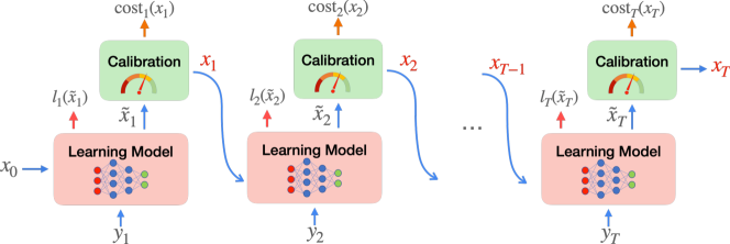
Figure 1. Illustration of EC-L2O. The ML-based optimizer $h_{W}$ is trained to minimize a weighted sum of two losses in view of the downstream expert calibrator $R_{\lambda}$. The expert calibrated actions $x_{1},\cdots,x_{T}$ are actually used by the online agent and directly determines the cost.

4.2.1. Online testing

At time step $t$, EC-L2O takes the available online contextual information $y_{t}$ as well as the previous action $x_{t-1}$, and outputs the current action $x_{t}$. More specifically, given $y_{t}$ and $x_{t-1}$, the ML-based optimizer $h$ predicts the action $\tilde{x}_{t}=h_{W}(y_{t},x_{t-1})$, which is then calibrated as the actual action $x_{t}$ by the expert algorithm $R$. Due to the presence of the expert calibrator $R$, the optimizer $R\circ h_{W}$ is more robust than simply using the ML predictions alone. This process follows a recurrent structure as illustrated in Fig. 1, where the base optimizers $R\circ h_{W}$ are concatenated one after another.

4.2.2. Offline training

The ML-based optimizer $h_{W}$ in EC-L2O is constructed using an ML model (e.g., neural network) with trainable weights $W$. But, unlike in $R\oplus h_{W}$ constructed using the naive two-stage approach in which the ML-based optimizer $h_{W}$ is trained as a standalone model to produce good online actions on its own, we train $h_{W}$ by considering the downstream expert calibration such that the average cost of the calibrated optimizer $R\circ h_{W}$ is minimized.

By analogy to a multi-layer neural network, we can view the added expert calibrator as another implicit “layer” following the ML predictions (Agrawal et al., 2019; Amos and Kolter, 2017). Unlike in a standard neural network where each layer has simple matrix computation and activation, the expert calibration layer itself is an optimization algorithm. Thus, the training process of $R\circ h_{W}$ in EC-L2O is much more challenging than that of a standalone ML-based optimizer used in the simple two-stage approach (i.e., $R\oplus h_{W}$).

The choices of the expert calibrator $R$ and loss function for training $R\circ h_{W}$ are critical to achieve our goal of reducing the average cost with good performance robustness. Next, we present the details of our expert calibrator and loss function.

4.3. Differentiable Expert Calibrator

We now design the expert calibrator that has good performance robustness and meanwhile is differentiable with respect to the ML predictions.

4.3.1. The necessity of being differentiable

When training an ML model, gradient-based backpropagation is arguably the state-of-the-art training method (Goodfellow et al., 2016). Also, Section 4.1 has already highlighted the drawback of training $h_{W}$ as a standalone model to minimize the pre-calibration cost without being aware of the downstream expert calibrator $R$. Therefore, when optimizing the weight $W$ of $h_{W}$ to minimize the post-calibration cost, we need to back propagate the gradient of $R$ with respect to the ML prediction output of $h_{W}$ (Agrawal et al., 2019; Amos and Kolter, 2017). Without the gradient, one may instead want to use some black-box gradient estimators like zero-order methods (Liu et al., 2020). Nonetheless, zero-order methods are typically computationally expensive due to the many samples needed to estimate the gradient, especially in our recurrent structure where the base optimizers are dependent on each other through time as illustrated in Fig. 1. Alternatively, one might want to pre-train a DNN to approximate the expert calibrator and then calculate the DNN’s gradients as substitutes of the expert calibrator’s gradients. Nonetheless, this alternative has its own limitation as well: many samples are required to pre-train the DNN to approximate the expert calibrator and, more critically, the gradient estimation error can still be large because a practical DNN only has finite generalization capability (Mohri et al., 2018). For these reasons, we would like our expert calibrator to be differentiable with respect to the ML predictions, in order to apply backpropagation and efficiently train $h_{W}$ while being aware of the downstream expert calibrator.

4.3.2. Expert calibrator

Our design of the expert calibrator is highly relevant to the emerging ML-augmented algorithm designs in the context of online convex optimization with switching costs (Antoniadis et al., 2020; Rutten et al., 2022). Commonly, the goal of ML-augmented algorithms is to achieve good competitive ratios in two cases: a bounded competitive ratio even when the ML predictions are bad (i.e., robustness), while being close to the ML predictions when they already perform optimally (i.e., consistency). Readers are referred to (Rutten et al., 2022) for formal definitions of robustness and consistency. Nonetheless, the existing algorithms (Antoniadis et al., 2020; Rutten et al., 2022; Christianson et al., 2022) view the ML-based optimizer as an exogenous black box without addressing how the ML models are trained. Moreover, they focus on switching costs in a metric space and hence do not apply to our setting where the switching cost is defined in terms of the squared Mahalanobis distance. For these reasons, we propose a new expert calibrator that generalizes the state-of-the-art expert algorithm — Regularized OBD (R-OBD) which matches the lower bound of any online algorithm for our problem setting (Goel et al., 2019) — by incorporating ML predictions.

The key idea of R-OBD is to regularize the online actions by encouraging them to stay close to the actions that minimize the current hitting cost at each time step. Neither future contextual information nor offline optimal actions are available in R-OBD. Thus, it uses the minimizer of the current hitting cost as an estimate of the offline optimal action to regularize the online actions, but clearly the minimizer of the current hitting cost can only provide limited information about the offline optimal since it ignores the switching cost. Thus, in addition to the minimizer of the current hitting cost, we view the ML predictions as another, albeit noisy, estimate of the offline optimal action. Our expert calibrator, called MLA-ROBD (ML-Augmented R-OBD) and described in Algorithm 1, generalizes R-OBD by introducing the ML predictions as another regularizer.

Algorithm 1 Machine Learning Augmented R-OBD (MLA-ROBD)

0:  $0<\lambda_{1}\leq 1$, $\lambda_{2}\geq 0$, $\lambda_{3}\geq 0$, the initialized action $x_{0}$.

1:  for $t=1,\cdots,T$

2:   Receive the context $y_{t}$.

3:   $v_{t}\leftarrow\arg\min_{x\in\mathcal{X}}f(x,y_{t})$ //Minimizer of the current hitting cost

4:   $\tilde{x}_{t}\leftarrow h_{W}(x_{t-1},y_{t})$ //ML prediction

5:   $x_{t}\leftarrow\arg\min_{x\in\mathcal{X}}f(x,y_{t})+\lambda_{1}c(x,x_{t-1})+\lambda_{2}c(x,v_{t})+\lambda_{3}c(x,\tilde{x}_{t})$ //Calibrating the ML prediction

In MLA-ROBD, at each time step $t$, the online action $x_{t}$ is chosen to minimize the weighted sum of the hitting cost, switching cost, the gap towards the current hitting cost’s minimizer $v_{t}$, and the newly added gap towards the ML prediction $\tilde{x}_{t}$. Compared to R-OBD, MLA-ROBD introduces a new regularizer $\lambda_{3}c(x,\tilde{x}_{t})$ in Line 5 of Algorithm 1 that keeps the online actions close to the ML predictions — the greater $\lambda_{3}\geq 0$, the stronger regularization. Thus, MLA-ROBD is more general than R-OBD, with tunable weights $\lambda_{1}$, $\lambda_{2}$ and $\lambda_{3}$ to balance the objectives. We also use $R_{\lambda}$ to represent MLA-ROBD to highlight that it is parameterized by $\lambda=(\lambda_{1},\lambda_{2},\lambda_{3})$.

More precisely, when $\lambda_{2}>0$ and $\lambda_{3}=0$, MLA-ROBD reduces to the standard R-OBD; when $\lambda_{1}=1$ and $\lambda_{2}=\lambda_{3}=0$, MLA-ROBD becomes the simple greedy algorithm which minimizes the current total cost (including the hitting and switching costs) at each step; and when $\lambda_{2}=0$ but $\lambda_{1}=\lambda_{3}=1$, MLA-ROBD will become the Follow the Prediction (FtP) algorithm studied in (Antoniadis et al., 2020).

4.3.3. Competitive ratio

Next, to show the advantage of MLA-ROBD in terms of the competitive ratio compared to pure ML predictions, we provide a competitive ratio upper bound in the following theorem, whose proof can be found in Appendix C.

Theorem 4.1.

Assume that the hitting cost function $f$ is $m$-strongly convex, and that the switching cost function $c$ is the Mahalanobis distance by matrix $Q$ with the minimum and maximum eigenvalues being $\frac{\alpha}{2}$ and $\frac{\beta}{2}$, respectively. If the ML predictions are $\rho$-accurate (Definition 3.1), MLA-ROBD has a competitive ratio upper bound of $\max\left(\frac{m+\lambda_{2}\beta}{m\lambda_{1}},1+\frac{\beta^{2}}{\alpha}\cdot\frac{\lambda_{1}}{(\lambda_{2}+\lambda_{3})\beta+m}\right)+\frac{\lambda_{3}\beta}{2\lambda_{1}}\rho$. Moreover, by optimally setting $\lambda_{2}=\frac{m\lambda_{1}}{2\beta}\left(\sqrt{\left(1+\frac{\beta}{m}\theta\right)^{2}+\frac{4\beta^{2}}{\alpha m}}+1-\frac{2}{\lambda_{1}}-\frac{\beta}{m}\theta\right)$ with $\theta=\frac{\lambda_{3}}{\lambda_{1}}$ being the trust parameter, the competitive ratio upper bound of MLA-ROBD becomes $1+\frac{1}{2}\left[\sqrt{(1+\frac{\beta}{m}\theta)^{2}+\frac{4\beta^{2}}{m\alpha}}-\left(1+\frac{\beta}{m}\theta)\right)\right]+\frac{\beta}{2}\theta\cdot\rho$.

Theorem 4.1 provides a dimension-free upper bound of the competitive ratio achieved by MLA-ROBD. Interestingly, although we have three weights $\lambda_{1},\lambda_{2}$ and $\lambda_{3}$, the optimal upper bound only depends on $\theta=\frac{\lambda_{3}}{\lambda_{1}}$, which we refer to as the trust parameter describing how much we trust the ML predictions.

In particular, when we completely distrust and ignore the ML predictions (i.e., $\theta=\frac{\lambda_{3}}{\lambda_{1}}=0$), we can recover the competitive ratio of standard R-OBD as $\frac{1}{2}(\sqrt{1+\frac{4\beta^{2}}{\alpha m}}+1)$ by setting $\lambda_{2}=\frac{m\lambda_{1}}{2\beta}\left(\sqrt{1+\frac{4\beta^{2}}{\alpha m}}+1-\frac{2}{\lambda_{1}}\right)$, which also matches the lower bound of the competitive ratio for any online algorithm (Goel et al., 2019). When we have full trust on the ML predictions (i.e., $\theta=\frac{\lambda_{3}}{\lambda_{1}}\to\infty$), the upper bound also increases to infinity unless the ML predictions are perfect with $\rho=0$. This is consistent with our discussion of the limitations of purely using ML predictions in Section 3.2.

When we partially trust the ML predictions (i.e., $0<\theta<\infty$), we can see that the upper bound increases with the prediction error $\rho$. In particular, when the ML predictions are extremely bad (i.e., $\rho\to\infty$), the competitive ratio of MLA-ROBD can also become unbounded. The non-ideal result is not a bug of MLA-ROBD or our proof technique, but rather due to the fundamental limit for the problem we study — as shown in Appendix B of (Rutten et al., 2022), no ML-augmented online algorithms could simultaneously achieve a consistency (i.e., competitive ratio for $\rho=0$) less than the optimal competitive ratio of R-OBD as well as a bounded robustness (i.e., competitive ratio for $\rho=\infty$). In our case, MLA-ROBD can benefit from good ML predictions and achieve a smaller competitive ratio than R-OBD when $\rho\to 0$, and thus its unbounded competitive ratio for $\rho=\infty$ is anticipated. Nonetheless, it is an interesting future problem to consider the other alternative, i.e., designing a new expert calibrator that achieves a bounded competitive ratio when $\rho=\infty$ without being able to exploit the benefit of good ML predictions when $\rho\to 0$.

More importantly, by properly setting the trust parameter $\theta=\frac{\lambda_{3}}{\lambda_{1}}$, the competitive ratio upper bound of MLA-ROBD can still be much smaller than the competitive ratio lower bound of purely using ML predictions (Lemma 3.2) when the ML prediction error $\rho$ is sufficiently large. This means that when the ML predictions are of a low quality, MLA-ROBD is guaranteed to be able to calibrate the predictions for significantly improving the competitive ratio.

To further illustrate this point, we show in Fig. 2 the competitive ratio lower bound of the pure ML-based optimizer $h$, the competitive ratio upper bounds of MLA-ROBD, and that of R-OBD under various prediction errors $\rho$. We can find that when the prediction error $\rho$ is small enough, the pure ML predictions are the best. But, this is certainly too opportunistic for a practical ML-based optimizer, whose actual testing performance cannot always be very good (i.e., $\rho$ is sufficiently small) due to the fundamental limitations discussed in Section 3.2. On the other hand, when the prediction error $\rho$ is large, expert calibration via MLA-ROBD is guaranteed to be better than the un-calibrated ML predictions. Additionally, introducing ML predictions with large errors in MLA-ROBD can increase the competitive ratio upper bound compared to the pure R-OBD expert algorithm that is independent of the prediction error. Nonetheless, by lowering the trust parameter, even ML predictions with errors up to a certain threshold are still beneficial to R-OBD and lead to a lower competitive ratio upper bound than R-OBD.

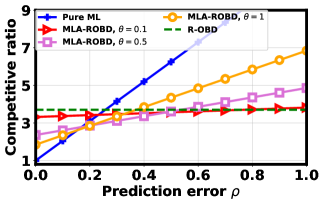
Figure 2. Illustration of competitive ratios of different algorithms.

In summary, when the prediction error is not too large, the competitive ratio upper bound of MLA-ROBD can be even smaller than that of R-OBD; when the prediction error is large enough, MLA-ROBD will be worse than R-OBD in terms of the competitive ratio upper bound due to the introduction of erroneous ML predictions, but, it can still be guaranteed to be much better than purely using ML predictions by setting a proper trust parameter. Based on these insights, we shall design our loss function for training the ML model $h_{W}$ in our expert-calibrated optimizer $R_{\lambda}\circ h_{W}$.

4.3.4. Regret

While we focus on the competitive ratio analysis, another metric commonly considered in the literature is the regret, which measures the difference between the cost achieved by an online algorithm and that by an oracle (Goel et al., 2019). Crucially, a desired result is that the regret grows sublinearly in time $T$, i.e., the time-averaged cost difference between an online algorithm and an oracle approaches zero as $T\to\infty$. Without ML predictions, the standard R-OBD can simultaneously achieve a sublinear regret while providing a dimension-free and bounded competitive ratio (Goel et al., 2019). Thus, it is interesting to see if MLA-ROBD, which incorporates ML predictions into R-OBD, can also achieve the same. To this end, we consider the $L$-constrained regret which, defined as follows, generalizes the classic static regret.

Definition 0 ($L$-constrained Regret).

For any problem instance with context $\bm{s}=(x_{0},\bm{y})$, suppose that an online algorithm makes actions $x_{1:T}=(x_{1},x_{2},\cdots,x_{T})$ and has a total cost of $cost(x_{1:T})=\sum_{t=1}^{T}f(x_{t},y_{t})+c(x_{t},x_{t-1})$. The $L$-constrained regret is defined as

(5) $$Regret(x_{1:T},x_{1:T}^{L})=cost(x_{1:T})-cost(x_{1:T}^{L}),$$

where $x_{1:T}^{L}$ denotes the actions made by the $L$-constrained optimal oracle that solves $x_{1:T}^{L}=\arg\min_{x_{1:T}}\sum_{t=1}^{T}f(x_{t},y_{t})+c(x_{t},x_{t-1})$ subject to $\sum_{t=1}^{T}c(x_{t},x_{t-1})\leq L$ and $cost(x_{1:T}^{L})$ is the corresponding total cost.

In the $L$-constrained regret, the oracle’s total switching cost is essentially constrained by $L$. When $L=0$, the $L$-constrained regret reduces to the classic static regret where the oracle is only allowed to make one static action; when $L$ increases, the oracle has more flexibility, making the $L$-constrained regret closer to the fully dynamic regret (Goel et al., 2019). As the regret compares an online algorithm against an $L$-constrained oracle, we also introduce $(L,L_{\rho})$-constrained prediction to quantify the ML prediction quality as follows.

Definition 0 ($(L,L_{\rho})$-constrained Prediction).

The ML predictions, denoted as $\tilde{x}_{1},\cdots\tilde{x}_{T}$, are said to be $(L,L_{\rho})$-constrained if the following is satisfied:

(6) $$\sum_{t=1}^{T}\|\tilde{x}_{t}-x_{t}^{L}\|^{2}\leq L_{\rho},$$

where $\|\cdot\|$ is the $l_{2}$-norm, and $x_{1}^{L},\cdots,x_{T}^{L}$ are the actions made by the $L$-constrained optimal oracle.

Note that, unlike $\rho$-accurate prediction (Definition 3.1) that is scale-invariant and normalized with respect to the unconstrained oracle’s optimal cost, the notion of $(L,L_{\rho})$-constrained prediction provides a different characterization of ML prediction quality by quantifying the absolute squared errors between ML predictions and the $L$-constrained oracle’s actions. Next, we provide an upper bound on the $L$-constrained regret in Theorem 4.4, whose proof can be found in Appendix D.

Theorem 4.4.

Assume that the hitting cost function $f$ is $m$-strongly convex, and that the switching cost function $c$ is the Mahalanobis distance by matrix $Q$ with the minimum and maximum eigenvalues being $\frac{\alpha}{2}>0$ and $\frac{\beta}{2}$, respectively. Additionally, assume that $\|Qx\|$ is bounded by $G<\infty$, the size/diameter of the feasible action set $\mathcal{X}$ is $\omega=\sup_{x,x^{\prime}\in\mathcal{X}}\|x-x^{\prime}\|$, and $\lambda_{1}\geq 1-\frac{m}{4\beta}$. For any problem instance and $(L,L_{\rho})$-constrained ML predictions, if $\lambda_{3}<\frac{\alpha}{\beta}$ and the total switching cost satisfies $\sum_{t=1}^{T}c(x_{t},x_{t-1})\leq L$, the $L$-constrained regret of MLA-ROBD satisfies $Regret(x_{1:T},x_{1:T}^{L})\leq\frac{\alpha}{\alpha-\lambda_{3}\beta}\big{(}(\lambda_{1}+\frac{m}{2\beta})G\sqrt{\frac{2TL}{\alpha}}+\lambda_{2}\frac{\beta T\omega^{2}}{2}+\frac{\lambda_{3}\beta}{2}L_{\rho}\big{)}$; otherwise, we have $Regret(x_{1:T},x_{1:T}^{L})\leq(\lambda_{1}+\frac{m}{2\beta})G\sqrt{\frac{2TL}{\alpha}}+(\lambda_{2}+\lambda_{3})\frac{\beta T\omega^{2}}{2}$. Moreover, by setting $\lambda_{2}=\eta_{2}(T,L,\omega,G)$ and $\lambda_{3}=\eta_{3}(T,L,\omega,G)$ such that $\lim_{T\rightarrow\infty}\left(\eta_{2}(T,L,\omega,G)+\eta_{3}(T,L,\omega,G)\right)\frac{\omega^{2}}{G}\sqrt{\frac{T}{L}}<\infty$, we have $Regret(x_{1:T},x_{1:T}^{L})=O(G\sqrt{TL})$.

In Theorem 4.4, we see that the $L$-constrained regret upper bound is increasing in both of the regularization weights $\lambda_{2}\geq 0$ and $\lambda_{3}\geq 0$. That is, by keeping the actions closer to the minimizer $v_{t}$ of the pure hitting cost and/or ML predictions $\tilde{x}_{t}$, the worst-case regret bound also increases. On the other hand, by Theorem 4.1, regularization by properly setting $\lambda_{2}>0$ and $\lambda_{3}>0$ is necessary to improve the competitive ratio performance and exploit the benefit of good ML predictions. Thus, Theorem 4.4 does not necessarily guarantee a sublinear regret when we aim at achieving the optimal competitive ratio. In fact, even without ML predictions, achieving both the optimal competitive ratio and a sublinear regret remains an open question (Goel et al., 2019). Nonetheless, Theorem 4.4 does show that by choosing sufficiently small $\lambda_{2}\geq 0$ and $\lambda_{3}\geq 0$, MLA-ROBD can achieve a sublinear regret $O(G\sqrt{TL})$. Together with the result in Theorem 4.1, MLA-ROBD also simultaneously achieves a dimension-free and conditionally-constant competitive ratio (conditioned on a finite prediction error $\rho$). Note finally that by setting $\lambda_{3}=0$, our result on the $L$-constrained regret reduces to the one for standard R-OBD (Goel et al., 2019).

4.4. Loss Function for Training

In Section 4.3, we have described our differentiable expert calibrator MLA-ROBD and shown its key advantage — improving performance robustness by lowering the worst-case competitive ratio of pure ML predictions. Besides the worst-case performance, another crucial goal is to achieve a low average cost, for which training the ML-based optimizer $h_{W}$ by explicitly considering the downstream calibrator $R_{\lambda}$ is essential (Section 4.1).

As illustrated in Fig. 1, at each time step $t=1,\cdots,T$, the calibrated action $x_{t}$ and its un-calibrated ML prediction $\tilde{x}_{t}$ can be expressed as

(7) $$x_{t}=R_{\lambda}(y_{t},x_{t-1},\tilde{x}_{t})\;\;\text{ and }\;\;\tilde{x}_{t}=h_{W}(y_{t},x_{t-1}),$$

where $R_{\lambda}$ is the expert calibrator (i.e., MLA-ROBD) and $h_{W}$ is the ML-based optimizer.

Naturally, our loss function for training should explicitly consider the expert-calibrated action $x_{t}$ to minimize the average cost, because it is $x_{t}$, rather than the un-calibrated ML prediction $\tilde{x}_{t}$, that is actually being used by the online agent and directly determines the cost. Thus, our loss function includes $\mathrm{cost}(R_{\lambda}\circ h_{W},\bm{s})$ to supervise the training process. On the other hand, if we only minimize $\mathrm{cost}(R_{\lambda}\circ h_{W},\bm{s})$ as our loss function, the ML-based optimzier $h_{W}$ is solely focusing on optimizing its un-calibrated prediction $\tilde{x}_{t}$ such that the post-calibration prediction $x_{t}$ achieves a low average cost. In other words, the un-calibrated prediction $\tilde{x}_{t}$ could be very bad if we were to directly use $\tilde{x}_{t}$ as the agent’s action. By Theorem 4.1, the competitive ratio upper bound achieved by MLA-ROBD linearly increases with respect to the ML prediction error $\rho$. This means that, if the pure ML predictions $\tilde{x}_{t}$ are of a very low quality and have a large prediction error, then the resulting competitive ratio of the expert-calibrated optimizer $R_{\lambda}\circ h_{W}$ can also be very large, compromising the worst-case performance robustness.

To address this issue and make the calibrator more useful, we define another loss for the ML-based optimizer as follows

(8) $$l(h_{W},\bm{s})=\mathrm{relu}\left(\frac{\sum_{t=1}^{T}\|\tilde{x}_{t}-x^{*}_{t}\|^{2}}{\mathrm{cost}(\pi^{*},\bm{s})}-\bar{\rho}\right),$$

where $\mathrm{relu}(x)=\max(x,0)$, $\tilde{x}_{t}$ is the output of $h_{W}$, $x^{*}_{t}$ is the offline optimal oracle’s action and $\bar{\rho}$ is a threshold of prediction error to determine whether a prediction is good enough. The added loss essentially regularizes the ML-based optimizer by encouraging it to predict actions with low prediction errors.

By balancing the two losses via a hyperparameter $\mu\in[0,1]$, our loss function for training the ML-based optimizer $h_{W}$ on a dataset $\mathcal{D}$ is given as follows:

(9) $$L_{\mathcal{D},R_{\lambda},\mu}(h_{W})=\mu\frac{1}{|\mathcal{D}|}\sum_{\bm{s}\in\mathcal{D}}l(h_{W},\bm{s})+(1-\mu)\frac{1}{|\mathcal{D}|}\sum_{\bm{s}\in\mathcal{D}}\mathrm{cost}(R_{\lambda}\circ h_{W},\bm{s}).$$

For the training loss function in Eqn. (9), by setting $\mu=1$, we recover the pure ML-based optimizer that can have a high cost when the testing input instances are far from the training instances. If $\mu=0$, we simply optimize the average post-calibration cost while ignoring the ML prediction error. Most typically, we set $\mu\in(0,1)$ to restrain the ML prediction error for meaningful expert calibration, and also to reduce the average cost.

The training dataset can be constructed based on historical problem instances and also possibly enlarged via data augmentation. As we directly optimize the ML model weights to minimize the sum of hitting and switching costs, we do not need labels (i.e., the offline oracle’s or an expert algorithm’s actions). Finally, note that we can also use held-out validation dataset to tune the hyperparameters (e.g., $\mu$, $\theta=\frac{\lambda_{3}}{\lambda_{1}}$, and learning rate) to achieve the most desired balance between the average cost and competitive ratio.

4.5. Differentiating the Expert Calibrator

We are now ready to derive the gradients of our differentiable expert calibrator MLA-ROBD shown in Algorithm 1. This is a crucial but non-trivial step for two reasons: first, unlike an explicit layer with simple matrix computation along with an activation function in a standard neural network, the expert-calibrator MLA-ROBD is essentially an implicit layer that executes an expert algorithm on its own (Kolter et al., lorg; Agrawal et al., 2019; Amos and Kolter, 2017); and second, due to the recurrent structure for sequential decision making, our backpropagation needs to be performed recurrently through time.

To efficiently train the ML-based optimizer $h_{W}$ in EC-L2O, we can apply various gradient-based algorithms such as SGD and Adam. These algorithms all require backpropagation and hence gradients of the objective in Eqn. (9). Thus, we need to differentiate $l(h_{W},\bm{s})$ and $\mathrm{cost}(R_{\lambda}\circ h_{W},\bm{s})$ with respect to the weight $W$ in the ML-based optimizer $h_{W}$. Next, we focus on the gradient of $\mathrm{cost}(R_{\lambda}\circ h_{W},\bm{s})$, while a similar method can be used to differentiate $l(h_{W},\bm{s})$.

By the expression of cost in Eqn. (1), the gradient of $\mathrm{cost}(R_{\lambda}\circ h_{W},\bm{s})$ given an input sequence $\bm{s}$ is written as

$$\nabla_{W}\mathrm{cost}(R_{\lambda}\circ h_{W},\bm{s})=\sum_{t=1}^{T}\nabla_{x_{t}}\left(f(x_{t}(W),y_{t})+c(x_{t}(W)-x_{t-1}(W))\right)\nabla_{W}R_{\lambda}(y_{t},x_{t-1}(W),\tilde{x}_{t}(W))$$

where the expert-calibrated action $x_{t}$ and the un-calibrated ML prediction $\tilde{x}_{t}$ are written as $x_{t}(W)$ and $\tilde{x}_{t}(W)$, respectively, to emphasize their dependence on the ML model weight $W$. Then, the gradient of the expert-calibrated action $x_{t}(W)$ with respect to $W$ is further written as

$$\begin{split}&\nabla_{W}R_{\lambda}(y_{t},x_{t-1}(W),\tilde{x}_{t}(W))\\ =&\nabla_{x_{t-1}}R_{\lambda}(y_{t},x_{t-1}(W),\tilde{x}_{t}(W))\nabla_{W}x_{t-1}(W)+\nabla_{\tilde{x}_{t}}R_{\lambda}(y_{t},x_{t-1}(W),\tilde{x}_{t}(W))\nabla_{W}\tilde{x}_{t}(W),\end{split}$$

where $\nabla_{W}x_{t-1}(W)=\nabla_{W}R_{\lambda}(y_{t-1},x_{t-2}(W),\tilde{x}_{t-1}(W))$ is the gradient of the expert-calibrated action with respect to $W$ at step $t-1$ and $\nabla_{W}\tilde{x}_{t}(W)=\nabla_{W}h_{W}(y_{t-1},x_{t-1}(W))$ is the gradient of the un-calibrated ML prediction.

Now, it remains to differentiate the implicit layer of the expert calibrator. We cannot directly differentiate the calibrator. But, since MLA-ROBD solves a convex optimization problem at each time step, we instead differentiate it by its optimum condition shown as follows

(10) $$\nabla_{x_{t}}f(x_{t},y_{t})+\lambda_{1}\nabla_{x_{t}}c(x_{t},x_{t-1})+\lambda_{2}\nabla_{x_{t}}c(x_{t},v_{t})+\lambda_{3}\nabla_{x_{t}}c(x_{t},\tilde{x}_{t})=0.$$

By taking the gradients for both sides and solving the obtained equation, we can derive the gradients of $R_{\lambda}$ with respect to $\tilde{x}_{t}$ and $x_{t-1}$ as

(11) $$\nabla_{\tilde{x}_{t}}R_{\lambda}(y_{t},x_{t-1},\tilde{x}_{t})=-\lambda_{3}Z_{t}^{-1}\nabla_{\tilde{x}_{t},x_{t}}c(x_{t},\tilde{x}_{t}),$$

(12) $$\nabla_{x_{t-1}}R_{\lambda}(y_{t},x_{t-1},\tilde{x}_{t})=-\lambda_{1}Z_{t}^{-1}\nabla_{x_{t-1},x_{t}}c(x_{t},x_{t-1}),$$

where $Z_{t}=\nabla_{x_{t},x_{t}}\left[f(x_{t},y_{t})+\lambda_{1}c(x_{t},x_{t-1})+\lambda_{2}c(x_{t},v_{t})+\lambda_{3}c(x_{t},\tilde{x}_{t})\right]$. Note that for our switching cost $c(x_{t},x_{t-1})=\left(x_{t}-x_{t-1}\right)^{\top}Q\left(x_{t}-x_{t-1}\right)$ defined in terms of the Mahalanobis distance with respect to $Q\in\mathcal{R}^{d\times d}$, we have $\nabla_{\tilde{x}_{t},x_{t}}c(x_{t},\tilde{x}_{t})=\nabla_{x_{t-1},x_{t}}c(x_{t},x_{t-1})=-2Q$ and $\nabla_{x_{t},x_{t}}c(x_{t},x_{t-1})=\nabla_{x_{t},x_{t}}c(x_{t},v_{t})=\nabla_{x_{t},x_{t}}c(x_{t},\tilde{x}_{t})=2Q$. The details of deriving the gradients in Eqn. (11) and Eqn. (12) are given in Appendix A.

5. Performance Analysis

To conclude the design of EC-L2O, we now analyze its performance in terms of the average cost as well as the tail cost ratio.

5.1. Average Cost

Average cost is a crucial metric and measures the performance of EC-L2O in many typical cases. Next, we analyze the average cost of EC-L2O by the generalization theory of statistical learning (Mohri et al., 2018). First, we define the optimal ML model weight $W^{*}$ in $h_{W}$ as follows.

Definition 0.

The optimal model weight $W^{*}$ in the ML-based optimizer $h_{W}$ of EC-L2O is defined as the minimizer of the expected training loss below:

(13) $$W^{*}=\arg\min_{W\in\mathcal{W}}\mu\mathbb{E}\left[l(h_{W},\bm{s})\right]+(1-\mu)\mathbb{E}\left[\mathrm{cost}(R_{\lambda}\circ h_{W},\bm{s})\right],$$

where $\mathcal{W}$ is the weight space depending on the model $h_{W}$ (e.g., DNN with a certain architecture) and the expectation is taken over the environment distribution $\mathbb{P}$ of the input instance $s$.

The optimal ML model, i.e., $h_{W^{*}}$, minimizes the weighted sum of the expected average cost of the expert-calibrated optimizer and the expectation of the ML prediction error $\rho$ (Definition 3.1) conditioned on $\rho\geq\bar{\rho}$. By setting $0<\mu<1$, $R_{\lambda}\circ h_{W^{*}}$ is essentially an online optimizer that minimizes the average cost while constraining the average prediction error $\rho$ conditioned on $\rho\geq\bar{\rho}$.

Next, we denote the optimal weight $\hat{W}^{*}$ that minimizes the empirical loss function in Eqn. (9) as $\hat{W}^{*}=\arg\min_{W\in\mathcal{W}}L_{\mathcal{D},R_{\lambda},\mu}(h_{W})$. Assuming that $\hat{W}\in\mathcal{W}$ is the model weight after training on the loss function in Eqn. (9), the training error on the training dataset $\mathcal{D}$ is denoted as

(14) $$\mathcal{E}_{\mathcal{D}}=L_{\mathcal{D},R_{\lambda},\mu}(h_{\hat{W}})-L_{\mathcal{D},R_{\lambda},\mu}(h_{\hat{W}^{*}}).$$

Now, we bound the expected average cost in the next theorem, whose proof is in Appendix E.

Theorem 5.2.

Assume that the dataset $\mathcal{D}$ is drawn from a distribution $\mathbb{P}^{\prime}$ and the environment distribution is $\mathbb{P}$. If $R_{\lambda}\circ{h}_{\hat{W}}$ is trained on the loss function in Eqn. (9), then with probability at least $1-\delta,\delta\in(0,1)$, we have

(15) $$\mathrm{AVG}(R_{\lambda}\circ{h}_{\hat{W}})\leq\mathrm{AVG}(R_{\lambda}\circ h_{W^{*}})+\frac{\mu}{1-\mu}\mathbb{E}\left[l(h_{W^{*}},\bm{s})\right]+\frac{1}{1-\mu}\mathcal{E}_{\mathcal{D}}+O\left(\sqrt{\frac{\log(1/\delta)}{|\mathcal{D}|}}+D(\mathbb{P},\mathbb{P}^{\prime})\right),$$

where $\mu$ is the trade-off parameter in Eqn. (13), $\mathcal{E}_{\mathcal{D}}$ is the training error in Eqn. (14), $|\mathcal{D}|$ is the number of instances in the training dataset, and $D(\mathbb{P},\mathbb{P}^{\prime})$ measures the distributional discrepancy between the distribution $\mathbb{P}^{\prime}$ from which the training instances are drawn from and the environment distribution $\mathbb{P}$.

Theorem 5.2 quantifies the average cost gap between the expert-calibrated learning model $R_{\lambda}\circ{h}_{\hat{W}}$ and the optimal optimizer $R_{\lambda}\circ h_{W^{*}}$. We can see that the gap is affected by the training-induced error $\mathcal{E}_{\mathcal{D}}$ and the generalization error induced by the distribution discrepancy between the training empirical distribution and the environment distribution $\mathbb{P}$. Also, the average cost bound has an additional term $\frac{\mu}{1-\mu}\mathbb{E}\left[l(h_{W^{*}},\bm{s})\right]$ which is caused by the first term in the training loss function in Eqn. (9). When $\mu=0$, although the additional term disappears and $R_{\lambda}\circ h_{\hat{W}}$ purely minimizes the average cost, the downside is that the pre-calibration ML prediction error could be empirically very high, which thus leads to a high post-calibration competitive ratio upper bound (Theorem 4.1). On the other hand, when $\mu=1$, the average cost is neglected during the training process and hence can be unbounded, which also implies that minimizing the average prediction error (and hence average ratio of the expert-calibrated optimizer’s cost to the offline optimal cost) does not necessarily lead to a lower average cost. In the bound in Eqn. (15), we also see the term $D(\mathbb{P},\mathbb{P}^{\prime})$ due to the training-testing distributional discrepancy. When $D(\mathbb{P},\mathbb{P}^{\prime})$ increases, although the average cost upper bound becomes larger, the benefit of expert calibration can be more significant compared to purely using ML predictions without calibration. This will be empirically validated in the next section and also can be explained as follows. By viewing EC-L2O as a two-layer model (i.e., the ML-based optimizer layer followed by the expert calibration layer), we see that the first layer is trainable, but the second layer is an expert algorithm that is specially designed for robustness and hence less vulnerable to the distributional shift. Thus, compared to a pure ML-based optimizer trained over the training distribution, EC-L2O with an additional expert calibration layer will be affected less by distributional shifts.

Finally, we explain the necessity of holistically training the expert-calibrated optimizer $R_{\lambda}\circ h_{\hat{W}}$ from the perspective of the generalization bound. For the sake of discussion, we assume $\mu=0$ in the loss function to focus on the average cost. If we follow the two-stage approach (Section 4.1) and train the ML-based optimizer as a standalone model with the weight $\tilde{W}$, we can derive a new generalization bound for the simple optimizer $R\oplus h_{\tilde{W}}$. The new generalization bound takes the same form of Eqn. (15) except for changing ML model weight from $\hat{W}$ to $\tilde{W}$. Specifically, the error term $\mathcal{E}_{\mathcal{D}}$ contained in the new bound becomes $L_{\mathcal{D},R_{\lambda},\mu}(h_{\tilde{W}})-L_{\mathcal{D},R_{\lambda},\mu}(h_{\hat{W}^{*}})$, where the ML model weight $\tilde{W}$ is trained separately to minimize the empirical pre-calibration loss while the term $L_{\mathcal{D},R_{\lambda},\mu}(h_{\tilde{W}})$ is evaluated based on the empirical post-calibration loss. On the other hand, the training error $\mathcal{E}_{\mathcal{D}}$ defined in Eqn. (14) contained in the generalization bound for $R_{\lambda}\circ{h}_{\hat{W}}$ in Eqn. (15) can be made sufficiently small by using state-of-the-art training algorithms (Goodfellow et al., 2016). Thus, by simply concatenating an ML-based optimizer $h_{\tilde{W}}$ with an expert calibrator $R$, the new optimizer $R\oplus h_{\tilde{W}}$ will likely have a larger generalization bound than $R_{\lambda}\circ{h}_{\hat{W}}$ due to the increased training error term.

5.2. Tail Cost Ratio

For $\rho$-accurate ML predictions, the competitive ratio of EC-L2O by using MLA-ROBD as the expert calibrator follows Theorem 4.1. While EC-L2O can lower the competitive ratio of R-OBD with good ML predictions, the worst-case competitive ratio keeps increasing as the ML prediction error $\rho$ increases. This result comes from the fundamental limit for our problem setting as shown in (Rutten et al., 2022). Thus, instead of considering the pessimistic worst-case competitive ratio of EC-L2O, we resort to the high-percentile tail ratio of the cost achieved by EC-L2O to that of the offline optimal oracle. We simply refer to this ratio as the tail cost ratio, which can provide a probabilistic view of the performance robustness of the algorithm.

Theorem 5.3.

Assume that the lower bound of the offline optimal cost is $\nu=\inf_{\bm{s}\in\mathcal{S}}\mathrm{cost}(\pi^{*},\bm{s})$ and the size of the action set $\mathcal{X}$ is $\omega=\sup_{x,x^{\prime}\in\mathcal{X}}\|x-x^{\prime}\|$. Given the same assumptions as in Theorem 5.2, with probability at least $1-\delta,\delta\in(0,1)$ regarding the randomness of input sequence $\bm{s}$, we have

(16) $$\frac{\mathrm{cost}(R_{\lambda}\circ h_{\hat{W}},\bm{s})}{\mathrm{cost}(\pi^{*},\bm{s})}\leq 1+\frac{1}{2}\left[\sqrt{(1+\frac{\beta}{m}\theta)^{2}+\frac{4\beta^{2}}{m\alpha}}-\left(1+\frac{\beta}{m}\theta)\right)\right]+\frac{\beta}{2}\theta\cdot\rho_{\mathrm{tail}},$$

where $\alpha$, $\beta$, $m$ and $\theta$ are explained in Theorem 4.1, and the tail ML prediction error $\rho_{\mathrm{tail}}=\bar{\rho}+\mathbb{E}\left[l(h_{W^{*}},\bm{s})\right]+\frac{1-\mu}{\mu}\mathbb{E}\left[\mathrm{cost}(R_{\lambda}\circ h_{W^{*}},\bm{s})\right]+\frac{1}{\mu}\mathcal{E}_{\mathcal{D}}+O\left(\sqrt{\frac{\log(2/\delta)}{|\mathcal{D}|}}\right)+O\left(D(\mathbb{P},\mathbb{P}^{\prime})\right)+O\left(\frac{\omega^{2}\sqrt{T}}{\nu}\|\Gamma\|\sqrt{\frac{1}{2}\log(\frac{4}{\delta})}\right)$, in which $\mu$, $\mathcal{D}$, $\mathcal{E}_{\mathcal{D}}$ and $D(\mathbb{P},\mathbb{P}^{\prime})$ are given in Theorem 5.2, $\bar{\rho}$ is the prediction error threshold parameter in Eqn. (8), $\Gamma$ is the mixing matrix with respect to a partition of the random sequence $\chi=\left\{\|\tilde{x}_{t}-x_{t}^{*}\|^{2}/\mathrm{cost}(\pi^{*},\bm{s}),t\in[T]\right\}$ (Paulin, 2015), and $\|\Gamma\|$ denotes the Frobenius norm.

The proof of Theorem 5.3 is available in Appendix F. The key insight is that for the hyperparameter $\mu\in(0,1]$ that balances the ML prediction error and the average cost in the training loss function in Eqn. (9), the tail ML prediction error $\rho_{\mathrm{tail}}$ is bounded, which, by Theorem 4.1, also leads to a bounded tail cost ratio. More precisely, as $\mu$ increases within $(0,1]$, more emphasis is placed on the ML prediction error in the training loss function in Eqn. (9). As a result, the tail ML prediction error also decreases, resulting in a reduced tail cost ratio. In the extreme case of $\mu=0$, the ML prediction error is completely neglected in the loss function in Eqn. (9) during the training process. Thus, as intuitively expected, the tail cost ratio can be extremely large and unbounded.

In Theorem 5.3, the ML prediction error $\rho_{\mathrm{tail}}$ is a crucial term affected by the size of action set $\omega=\sup_{x,x^{\prime}\in\mathcal{X}}\|x-x^{\prime}\|$, the lower bound of the offline optimal cost $\nu=\inf_{\bm{s}\in\mathcal{S}}\mathrm{cost}(\pi^{*},\bm{s})$, and the Frobenius norm of the mixing matrix $\Gamma$ due to the McDiarmid’s inequality for dependent variables (Paulin, 2015). Among them, the mixing matrix $\Gamma$ is an upper diagonal matrix, whose dimension is the length of the corresponding partition of $\chi$. The mixing matrix relies on the distribution of $\chi$ and its norm affects the degree of concentration of the sequence $\chi$. Specifically, a sequence with independent variables has a partition with the identity matrix as the mixing matrix, and a uniformly ergodic Markov chain has a partition with the mixing matrix $\Gamma_{i,j}\leq\epsilon^{\mathrm{relu}(j-i-1)}\mathds{1}(j\geq i)$ where $\epsilon\in[0,1)$ is a parameter determined by the partition (Paulin, 2015). Given a fixed set of other terms, the less concentration of the sequence $\chi$ (or higher $\|\Gamma\|$), the higher tail ML prediction error as well as the higher tail cost ratio.

By setting $\mu\in(0,1)$, we highlight the importance of considering the loss function in Eqn. (9) that includes two different losses — one for the ML-based optimizer to have a low average prediction error, and the other one for the post-calibration ML calibrations to have a low average cost. Albeit weaker than the worst-case competitive ratio, the result in Theorem 5.3 is also crucial and provides a probabilistic performance robustness of EC-L2O.

6. Case Study: Sustainable Datacenter Demand Response

In this section, we conduct a case study and perform simulations on the application of sustainable datacenter demand response to validate the design of EC-L2O. Importantly, our results demonstrate that EC-L2O can achieve a lower average cost, as well as an empirically lower competitive ratio, than several baseline algorithms. This nontrivial result is due in great part to our differentiable expert calibrator and loss function designed based on our theoretical analysis.

6.1. Application

Fueled the demand for sustainability, green renewables, such as wind and solar energy, have been increasingly adopted in today’s power grids. Nevertheless, since renewables are not as stable as traditional energy sources and can fluctuate rapidly over time, the integration of renewables into the power grid poses substantial challenges to meet the time-varying demand. Consequently, this calls for more demand response resources — energy loads that can flexibly respond to the fluctuating supplies — in order to balance the supply and demand at all times (Sheppy et al., 2011; U.S. DoE, 2006).

On the other hand, warehouse-scale datacenters are traditionally viewed as energy hogs, taking up a huge load in power grids (Wierman et al., 2014). Nonetheless, this negative view has been quickly changing in recent years. Specifically, unlike traditional loads, datacenters have great flexibility to adjust their energy demands using a wide range of control knobs at little or even no cost, such as turning off unused servers, spatially shifting workloads to elsewhere, deferring non-urgent workloads, and setting a higher cooling temperature (Ghatikar et al., 2012). Compounded by the megawatt scale, these knobs can shed the datacenter energy consumption by a significant amount and make datacenters valuable demand response resources. In fact, an increasingly larger number of datacenters have already been actively participating in demand response programs that help stabilize and green the power grid (Liu et al., 2014; Sun et al., 2016).

We consider the application of sustainable datacenter demand response to facilitate integration of rapidly fluctuating renewables, including wind power and solar power, into a micro power grid (a.k.a. microgrid) serving the data center. More formally, the wind power $P_{\mathrm{wind},t}$ and solar power $P_{\mathrm{solar},t}$ at each time step $t$ both rely on the corresponding weather conditions. Here, we use empirical equations to model the wind and solar renewables. For wind power, the amount of energy generated at step $t$ is modeled by using the equation in (Sarkar and Behera, 2012) as $P_{\mathrm{wind},t}=\frac{1}{2}\kappa_{\mathrm{wind}}\varrho A_{\mathrm{swept}}V_{\mathrm{wind},t}^{3}$, where $\kappa_{\mathrm{wind}}$ is the conversion efficiency (%) of wind power, $\varrho$ is the air density ($kg/m^{3}$), $A_{\mathrm{swept}}$ is the swept area of the turbine ($m^{2}$), and $V_{\mathrm{wind},t}$ is the wind speed ($kW/m^{2}$) at time step $t$. For solar power, the amount of energy generated at step $t$ is modeled based on (Wan et al., 2015) as $P_{\mathrm{solar},t}=\frac{1}{2}\kappa_{\mathrm{solar}}A_{\mathrm{array}}I_{\mathrm{rad},t}(1-0.05*(\mathrm{Temp}_{t}-25))$, where $\kappa_{\mathrm{solar}}$ is the conversion efficiency (%) of the solar panel, $A_{\mathrm{array}}$ is the array area ($m^{2}$), and $I_{\mathrm{rad},t}$ is the solar radiation ($kW/m^{2}$) at time step $t$, and $\mathrm{Temp}_{t}$ is the temperature (^∘C) at step $t$. At time step $t$, the total energy generated by the renewables $P_{\mathrm{r},t}=P_{\mathrm{wind},t}+P_{\mathrm{solar},t}$.

We assume that at each step, the datacenter offers demand response to compensate the microgrid’s power shortage $y_{t}=\max(P_{\mathrm{s},t}-P_{\mathrm{r},t},0)$ (i.e., the net amount of energy shedding needed from the datacenter), where $P_{\mathrm{s},t}$ is the power shortage before renewable integration. The amount of energy load shedding offered by the datacenter is the action $x_{t}$. We model the hitting cost as the squared norm of the difference between the action $x_{t}$ and the context $y_{t}$, i.e. $f(x_{t},y_{t})=\frac{1}{2}\|x_{t}-y_{t}\|^{2}$, which captures the quadratic cost incurred by the microgrid due to the actual supply-demand mismatch (Liu et al., 2014). Additionally, we model the switching cost by a scaled and squared norm of the difference between two consecutive actions, i.e. $c(x_{t},x_{t-1})=\frac{\alpha}{2}\|x_{t}-x_{t-1}\|^{2}$. This cost comes from the changes of demand response knobs in the datacenter, e.g., setting different supply air temperature to adjust energy shedding (Sharma et al., 2005). The goal of sustainable datacenter demand response is to make online actions to minimize the total cost in Eqn. (1).

6.2. Simulation Settings

We give the details about the settings in our simulation. The switching cost parameter is set as $\alpha=10$. To calculate the renewable energy, we set the parameters for wind power as $\kappa_{\mathrm{wind}}=30\%$, $\varrho=1.23kg/m^{3}$, $A_{\mathrm{swept}}=500,000m^{2}$. The wind speed data is collected from the National Solar Radiation Database (Sengupta et al., 2018), which contains hourly data for the year of 2015. Additionally, we set the parameters for solar power as $\kappa_{\mathrm{wind}}=10\%$, $A_{\mathrm{array}}=10,000m^{2}$. The temperature data and the Global Horizontal Irradiance (GHI) data are also from the National Solar Radiation Database (Sengupta et al., 2018). For both temperature and GHI data, we use hourly data for the year of 2015. A snapshot of the context sequence $y_{t}$ is shown in Fig. 3.

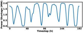
Figure 3. A snapshot of the context $y_{t}$.

We use the hourly data of the first two months and data augmentation to generate a training dataset with 1400 sequences, each with 24 hours. The data of the third month is used for validation and hyperparameter tuning. The data of the remaining nine months is used as the testing dataset. Each problem instance is $T=24$ hours. We perform continuous testing by using the action of the previous testing instance as the initial action of the current testing instance. Fig. 4 visualizes the t-SNE of discrepancy between training and testing distributions (Maaten and Hinton, 2008). We can see that the testing distribution shifts from the training distribution, which we refer to as out-of-distribution testing and is common in practice since the distribution of (finite) training samples may not truly reflect the testing distribution.

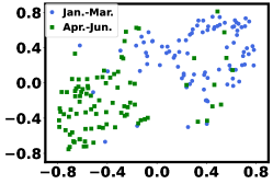
(a) Testing of Apr. to Jun.

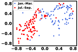
(b) Testing of Jul. to Sep.

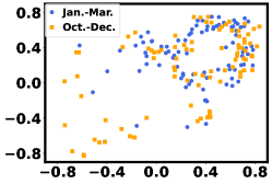
(c) Testing of Oct. to Dec.

Figure 4. t-SNE of distribution discrepancies between training months (January to March) and testing months.

In our recurrent structure, the ML model $h_{W}$ in each base optimizer includes 3 layers, each having 10 neurons. We use $\mathrm{relu}$ activation and train the model weight using Adam optimization.

6.3. Baseline Algorithms

We compare EC-L2O with several baselines including experts and ML-based algorithms. The baselines are summarized as below.

$\bullet$ Offline optimal oracle (Oracle): The offline optimal oracle has access to the complete context information in advance and produces the optimal solution.

$\bullet$ Regularized Online Balance Descent (R-OBD): R-OBD is the state-of-the-art expert algorithm that matches the lower bound of any online algorithms in terms of the competitive ratio (Goel et al., 2019). It uses the minimizer of the current hitting cost as a regularizer for online actions. By setting $\lambda_{3}=0$, the expert calibrator MLA-ROBD reduces to R-OBD.

$\bullet$ Pure ML-based Optimizer (PureML): PureML uses the same recurrent neural network as EC-L2O, but it is trained as a standalone optimizer without considering the downstream expert calibrator. More specifically, we consider the loss function $\kappa\frac{\mathrm{cost}(h_{W},\bm{s})}{\mathrm{cost}(\pi^{*},\bm{s})}+(1-\kappa)\mathrm{cost}(h_{W},\bm{s})$ for the PureML model $h_{W}$, where $\kappa\in[0,1]$ balances the cost ratio loss and the average cost loss. Specifically, when $\kappa=0$, we denote the PureML model as PureML-0, which is trained to minimize the average cost as in the standard L2O technique (Chen et al., 2017).

$\bullet$ PureML with Dynamic Switching (Switch): A switching-based online algorithm dynamically switches between an individually robust expert and ML predictions. The two most relevant switching-based online algorithms (Antoniadis et al., 2020; Rutten et al., 2022) consider switching costs in a metric space and hence are not directly applicable for our squared switching costs. Here, we modify Algorithm 1 in (Antoniadis et al., 2020) by switching between R-OBD and pre-trained PureML with $\kappa=0$ (PureML-0) based on a parameterized threshold $\gamma$ that progressively increases itself for each occurrence of switch. This essentially follows the two-stage approach discussed in Section 4.1, and is simply referred to as Switch. Since the switching algorithm in (Rutten et al., 2022) relies on triangle inequality of switching costs in a metric space, it is highly non-trivial to adapt the algorithm to our setting. Thus, we exclude it from our comparison.

$\bullet$ PureML with MLA-ROBD (MLA-ROBD): To highlight the importance of training the ML-based optimizer $h_{W}$ by taking into account the downstream calibrator, we apply predictions of the pre-trained PureML-0 in MLA-ROBD. We simply refer to the whole algorithm as MLA-ROBD.

Note that the all the costs shown in our results are normalized by the average cost achieved by the offline optimal oracle. In Figs. 5(a) and 5(b), the default hyperparameters used for the algorithms under consideration are $\kappa=0$ for PureML, $\gamma=1.5$ for Switch, $\theta=0.3$ for MLA-ROBD, and $\theta=0.5$ and $\mu=0.6$ for EC-L2O. The hyperparameters for R-OBD and $\lambda_{2}$ in MLA-ROBD and EC-L2O are optimally set according to Theorem 4.1.

6.4. Results

We present our results of the average cost and competitive ratio as follows. Note that the empirical regret result is omitted, because it is already implicitly reflected by the average cost normalized with respect to the unconstrained optimal oracle’s cost (e.g., a normalized average cost of 1.2 means that the normalized average regret is 0.2).

First, for the default hyperparameters, the normalized average costs and empirical competitive ratios of EC-L2O and baselines are shown in Fig. 5(a) and Fig. 5(b), respectively. We can observe that the R-OBD achieves a very low competitive ratio, which is close to the competitive ratio lower bound in (Goel et al., 2019). However, R-OBD has a very large average cost since it does not exploit any additional information such as statistical information of testing instances or ML predictions.

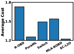
(a) Average cost

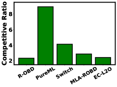
(b) Competitive ratio

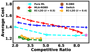
(c) AVG vs. CR tradeoff

Figure 5. Performance comparison.

By exploiting the input distributional information, PureML can reduce the average cost effectively, but due to the limitations of ML, it has unsatisfactory worst-case performance — an undesirably high competitive ratio. As ML-augmented online algorithms, Switch and MLA-ROBD can effectively lower the competitive ratio, but their average costs are much worse than PureML. The reasons are two-fold: (1) the competitive ratios in these algorithms are often loose and hence may not reflect the true empirical performance; and (2) the ML-based optimizer (PureML in this case) used by these algorithms is trained to minimize the pre-calibration cost using the standard practice of L2O as a standalone optimizer without being aware of the downstream expert algorithm. This highlights that we cannot simply view the ML-based optimizer as an exogenous blackbox as in the existing ML-augmented algorithms (Antoniadis et al., 2020).

When the training and testing distributions are well consistent, one may expect PureML to have the lowest average cost, if the ML model has sufficient capacity and is well trained with a large number of training samples. Nonetheless, for out-of-distribution testing in practice as shown in Fig. 4, the number of hard testing samples for PureML is no longer non-negligible. As a consequence, PureML may not perform the best in terms of the average cost. Interestingly, we see from Fig. 5 that EC-L2O can achieve an average cost even lower than PureML while keeping a competitive ratio that is not much higher than R-OBD. This demonstrates the effectiveness of EC-L2O in terms of reducing the average cost while restraining the empirical competitive ratio. On the one hand, while the ML model in EC-L2O is still vulnerable to out-of-distribution samples, the downstream expert calibrator does not depend on the training data and is provably more robust. Thus, along with our holistic training to minimize the post-calibration cost, EC-L2O results in a lower average cost than PureML in the presence of training-testing distribution discrepancies. On the other hand, although the competitive ratio of EC-L2O is not theoretically upper bounded, the training loss function in Eqn. (9) includes a loss of the ML prediction error which encourages the ML-based optimizer to have low prediction errors. Thus, by Theorem 4.1, this empirically reduces the competitive ratio achieved by EC-L2O.

Next, in Fig. 5(c), we show the trade-off between the average cost and competitive ratio by varying the respective hyperparameters that control the trade-off for different algorithms. For each trade-off curve, we only keep the Pareto boundary. By setting the trust parameter to a low value of $\theta=0.2$, the leftmost point of MLA-ROBD can be even better than the pure R-OBD due to the introduction of ML predictions that are good in most cases. This is also reflected in Theorem 4.1 and Fig. 2. On the other hand, by $\theta=5$, ML predictions play a bigger role and MLA-ROBD approaches PureML with $\kappa=0$ (labeled as star). PureML can balance the average cost and the competitive ratio by adjusting the trade-off parameter $\kappa$. However, PureML only optimizes the trade-off performance based on an offline training dataset without an expert calibration layer, and hence it suffers from various limitations including generalization error, limited network capacity, error from testing distributional shifts. Although Switch and MLA-ROBD can achieve reasonably low competitive ratios, their average costs are higher than that of PureML and EC-L2O. On the other hand, EC-L2O with two different trust parameters $\theta=0.4$ and $\theta=0.5$ can achieve the empirically best Pareto front among all the algorithms: given an average cost, EC-L2O has lower competitive ratios. Also, we can find that if the trust parameter $\theta$ is higher, the Pareto front becomes slightly better since more trust is given to the already-performant ML model. Nonetheless, we cannot fully trust the ML predictions by setting $\theta\to\infty$, which would otherwise significantly increase the competitive ratio. From Fig. 5(c), we also see empirically that the trade-off curve for EC-L2O is concentrated within a small region under different hyperparameters (e.g., $\mu$ and $\theta=\frac{\lambda_{3}}{\lambda_{1}}$), showing that EC-L2O is not as sensitive to the hyperparameters as other algorithms under comparison.

Finally, we compare the tail cost ratios of algorithms at higher percentile greater than 99% in Fig. 6. We can observe that EC-L2O achieves lower cost ratios than PureML, especially at percentile close to 100%. Also, EC-L2O has comparable cost ratios with ML-augmented algorithms, i.e., Switch and MLA-ROBD. This empirically confirms the conclusion in Theorem 5.3 that by training on Eqn. (8) with $\mu>0$, EC-L2O can constrain the cost ratio at high percentile, thus achieving a good tail robustness.

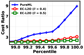
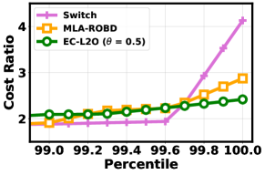
Figure 6. Tail cost ratio comparison between different algorithms

7. Related Works

The set of expert-designed algorithms for online convex optimization with switching costs and other variant problems (e.g., convex boday chasing (Friedman and Linial, 1993) and metrical task system (Blum and Burch, 2000)) have been growing all the time (Lin et al., 2011; Shi et al., 2020; Chen et al., 2018; Zhang et al., 2021a). For example, some prior studies have considered online gradient descent (OGD) (Zinkevich, 2003; Comden et al., 2019), online balanced descent (OBD) (Chen et al., 2018), and regularized OBD (R-OBD) (Goel et al., 2019). Typically, these algorithms are developed based on classic optimization frameworks and offer guaranteed worst-case performance robustness in terms of the competitive ratio. But, they may not have good cost performance in typical cases, thus potentially resulting in a high average cost.

Additionally, some other studies have also incorporated ML prediction of future cost parameters into the algorithm design under various settings. Examples include receding horizon control (RHC) (Comden et al., 2019) committed horizon control (CHC) (Chen et al., 2016), receding horizon gradient descent (RHGD) (Li et al., 2020, 2019), and adaptive balanced capacity scaling (ABCS) (Rutten and Mukherjee, 2022). The goal of these algorithms is still to achieve a low/bounded competitive ratio (or regret) in the presence of possibly large context prediction errors, while the average cost is left under-explored.

More recently, by combining ML-predicted actions with expert knowledge, ML-augmented algorithm designs have been emerging in the context of online convex optimization (or relevant problems such as convex body/function chasing) with switching costs (Antoniadis et al., 2020; Rutten et al., 2022; Christianson et al., 2022). They focus on switching costs in a metric space while we consider squared switching costs. Moreover, the existing studies focus on designing the expert calibration rule to achieve a low competitive ratio, and hence take a rather simplified view of the ML-based actions — the actions come from a black-box ML model. Thus, how to design the ML-based optimizer that provides predictions to the downstream expert algorithm still remains open. Simply following a two-stage approach in Section 4.1 can provide unsatisfactory performance in terms of the average cost, compared to the pure standalone ML-based optimizer that is trained for good average cost performance on its own. Thus, in this paper, our proposal of EC-L2O addresses a crucial yet unstudied challenge in the emerging context of ML-augmented algorithm design: how to learn for online convex optimization with switching costs in the presence of a downstream expert?

EC-L2O also intersects with the quickly expanding area of learning to optimize (L2O), which pre-trains an ML-based optimizer to directly solve optimization problems (Li and Malik, 2017; Chen et al., 2021; Wichrowska et al., 2017). Most commonly, L2O focuses on speeding up the computation for otherwise computationally expensive problems, such as as DNN training (Andrychowicz et al., 2016), nonconvex optimization in interference channels (Liang et al., 2020; Cui et al., 2019) and combination optimization (Dai et al., 2017). Moreover, ML-based optimizers have also been integrated into traditional algorithmic frameworks for faster and/or better solutions (Chen et al., 2021; Kolter et al., lorg). But, these studies are dramatically different due to their orthogonal design goals and constraints.

Studies that apply L2O to solve difficult online optimization problems where the key challenge comes from the lack of complete offline information have been relatively under-explored. In (Kong et al., 2019), an ML model is trained as a standalone end-to-end solution for a small set of classic online problems, such as online knapsack. In (Du et al., 2022) proposes adversarial training based on generative adversarial networks to solve online resource allocation problems. But, such an end-to-end ML-based optimizer can have bad performance without provably good robustness. While feeding the predictions of a pre-trained ML model directly into an expert calibrator can improve the robustness, the average cost performance can be significantly damaged due to the siloed two-stage approach.

In the recent “predict-then-optimize” and decision-focused learning framework (Wang et al., 2021; Liu and Grigas, 2021; Wilder et al., 2019; Elmachtoub and Grigas, 2017), auxiliary contextual information is predicted based on additional input features by taking into account the downstream optimizer in order to minimize the overall decision cost. A key research problem is to differentiate the optimizer with respect to the predicted contextual information in order to facilitate the backpropagation process for efficient training (Agrawal et al., 2019; Amos et al., 2018; Amos and Kolter, 2017). Nonetheless, these studies typically focus on the prediction step while considering an existing optimizer with the goal of optimizing the average performance, whereas we consider multi-step online optimization and propose a new expert calibrator to optimize the average performance with provably improved robustness. Additionally, although the optimizer produces actions based on the predicted contextual information, the “predict-then-optimize” framework still uses the true contextual information to evaluate the cost; by contrast, we directly utilize ML together with an expert calibrator to produce online actions and evaluate the total cost, and the notion of “true” actions does not apply in our problem.

Finally, a small set of recent studies (Anand et al., 2020, 2021; Du et al., 2021) have begun to study “how to learn” in ML-augmented algorithm designs for different goals. For example, (Du et al., 2021) designs an alternative ML model for the count-min sketch problem, while (Anand et al., 2021) considers general online problems and uses ML (i.e., regression) to minimize the average competitive ratio without considering the average cost. Our work is novel in multiple aspects, including the problem setting, expert calibrator, loss function design, backpropagation process and performance analysis.

8. Conclusion

In this paper, we study online convex optimization with switching costs. We show that by using the standard practice of training an ML model as a standalone optimizer, ML-augmented online algorithms can significantly hurt the average cost performance. Thus, we propose EC-L2O, which trains an ML-based optimizer by explicitly taking into account the downstream expert calibrator. We design a new differentiable expert calibrator, MLA-ROBD, that generalizes R-OBD and offers a provably better competitive ratio than pure ML predictions when the prediction error is large. We also provide theoretical analysis for EC-L2O, highlighting that the high-percentile tail cost ratio can be bounded. Finally, we test EC-L2O by running simulations for sustainable datacenter demand response, showing that that EC-L2O can empirically achieve a lower average cost as well as a lower competitive ratio than the existing baseline algorithms.

Appendix

Appendix A Additional Details of Differentiating the Calibrator

We now differentiate the output $x_{t}$ of the calibrator MLA-ROBD with respect to its inputs $\tilde{x}_{t}$ and $x_{t-1}$. By the optimum condition of the convex optimization to calculate $x_{t}$ in Algorithm 1, we have

(17) $$\nabla_{x_{t}}f(x_{t},y_{t})+\lambda_{1}\nabla_{x_{t}}c(x_{t},x_{t-1})+\lambda_{2}\nabla_{x_{t}}c(x_{t},v_{t})+\lambda_{3}\nabla_{x_{t}}c(x_{t},\tilde{x}_{t})=0.$$

To derive the gradient of $x_{t}=R_{\lambda}(y_{t},x_{t-1},\tilde{x}_{t})$ with respect to $\tilde{x}_{t}$, we take gradient for both sides of Eqn. (17), and get

(18) $$\begin{split}&\left(\nabla_{x_{t},x_{t}}f(x_{t},y_{t})+\lambda_{1}\nabla_{x_{t},x_{t}}c(x_{t},x_{t-1})+\lambda_{2}\nabla_{x_{t},x_{t}}c(x_{t},v_{t})+\lambda_{3}\nabla_{x_{t},x_{t}}c(x_{t},\tilde{x}_{t})\right)\nabla_{\tilde{x}_{t}}R_{\lambda}(y_{t},x_{t-1},\tilde{x}_{t})\\ &+\lambda_{3}\nabla_{\tilde{x}_{t},x_{t}}c(x_{t},\tilde{x}_{t})=0,\end{split}$$

where $\nabla_{x_{b},x_{a}}$ means first taking gradient with respect to $x_{a}$, and then taking gradient with respect to $x_{b}$. Denote $Z_{t}=\nabla_{x_{t},x_{t}}f(x_{t},y_{t})+\lambda_{1}\nabla_{x_{t},x_{t}}c(x_{t},x_{t-1})+\lambda_{2}\nabla_{x_{t},x_{t}}c(x_{t},v_{t})+\lambda_{3}\nabla_{x_{t},x_{t}}c(x_{t},\tilde{x}_{t})$. Due to the assumption that $f(x_{t},y_{t})$ and $c$ are strongly with respect to $x_{t}$, we have $Z_{t}$ is positive definite and invertible and so

(19) $$\nabla_{\tilde{x}_{t}}R_{\lambda}(y_{t},x_{t-1},\tilde{x}_{t})=-\lambda_{3}Z_{t}^{-1}\nabla_{\tilde{x}_{t},x_{t}}c(x_{t},\tilde{x}_{t}).$$

Similarly to derive the gradient of $x_{t}=R_{\lambda}(y_{t},x_{t-1},\tilde{x}_{t})$ with respect to $x_{t-1}$, we take gradient for both sides of Eqn. (17), and get

(20) $$\begin{split}&\left(\nabla_{x_{t},x_{t}}f(x_{t},y_{t})+\lambda_{1}\nabla_{x_{t},x_{t}}c(x_{t},x_{t-1})+\lambda_{2}\nabla_{x_{t},x_{t}}c(x_{t},v_{t})+\lambda_{3}\nabla_{x_{t},x_{t}}c(x_{t},\tilde{x}_{t})\right)\nabla_{x_{t-1}}R_{\lambda}(y_{t},x_{t-1},\tilde{x}_{t})\\ &+\lambda_{1}\nabla_{x_{t-1},x_{t}}c(x_{t},x_{t-1})=0.\end{split}$$

Thus, we have

(21) $$\nabla_{x_{t-1}}R_{\lambda}(y_{t},x_{t-1},\tilde{x}_{t})=-\lambda_{1}Z_{t}^{-1}\nabla_{x_{t-1},x_{t}}c(x_{t},x_{t-1}).$$

Appendix B Proof of Lemma 3.2

Proof.

Denote $\{\tilde{x}_{1},\cdots,\tilde{x}_{T}\}$ as the $\rho$-accurate predictions of an ML model $h_{W}$. Let the output of the offline optimal policy $\pi^{*}$ be $\{x_{1}^{*},x_{2}^{*},\cdots,x_{T}^{*}\}$. If the competitive ratio of the ML model is $\eta$, then by the definition of competitive ratio, we have $\mathrm{cost}(h_{W},\bm{s})\leq\eta\mathrm{cost}(\pi^{*},\bm{s})$, for any $\bm{s}\in\mathcal{S}$ such that the ML prediction is $\rho$-accurate. Thus, we prove the lower bound of the competitive ratio of the $\rho$-accurate ML model by finding a sequence $\bm{s}$ with predicted action sequence such that $\sum_{t=1}^{T}\|\tilde{x}_{t}-x^{*}_{t}\|\leq\rho\mathrm{cost}(\pi^{*},\bm{s})$ and the cost ratio $\frac{\mathrm{cost}(h_{W},\bm{s})}{\mathrm{cost}(\pi^{*},\bm{s})}\geq 1+\frac{m+2\alpha}{2}$.

We find the sequence of ML predictions by replacing the first action of the offline-optimal action sequence with $\hat{x}_{1}\in\mathcal{X},||\hat{x}_{1}-x_{1}^{*}||^{2}=\rho cost(\pi^{*},\bm{s})$, i.e. $\{\tilde{x}_{1},\cdots,\tilde{x}_{T}\}=\{\hat{x}_{1},x_{2}^{*},\cdots,x_{T}^{*}\}$. We then prove that the cost ratio of this ML prediction sequence is at least $1+\frac{m+2\alpha}{2}$.

Since $\{x_{1}^{*},x_{2}^{*},\cdots,x_{T}^{*}\}$ is the offline optimal sequence that minimizes Eqn. (1), then $x_{1}^{*}$ must be the minimizer of the function $p(x)=f(x,y_{1})+c(x,x_{0})+c(x,x_{2}^{*})$. Since the hitting cost $f(x,y)$ is $m$-strongly convex in terms of $x$, and the switching cost $c(x_{a},x_{b})$ is $\alpha$-strongly convex in terms of $x_{a}$, we have

(22) $$\nabla p(x_{1}^{*})=\nabla_{x_{1}^{*}}f(x_{1}^{*},y_{1})+\nabla_{x_{1}^{*}}c(x_{1}^{*},x_{0})+\nabla_{x_{1}^{*}}c(x_{1}^{*},x_{2}^{*})=0.$$

Thus we have

(23) $$\begin{split}&\mathrm{cost}(h_{W},\bm{s})-\mathrm{cost}(\pi^{*},\bm{s})\\ =&p(\hat{x}_{1})-p(x^{*}_{1})\\ =&f(\hat{x}_{1},y_{1})-f(x_{1}^{*},y_{1})+c(x_{0},\hat{x}_{1})-c(x_{0},x_{1}^{*})+c(\hat{x}_{1},x_{2}^{*})-c(x_{1}^{*},x_{2}^{*})\\ \geq&(\nabla_{x_{1}^{*}}f(x_{1}^{*},y_{1})+\nabla_{x_{1}^{*}}c(x_{1}^{*},x_{0})+\nabla_{x_{1}^{*}}c(x_{1}^{*},x_{2}^{*}))^{T}\cdot(\hat{x}_{1}-x_{1}^{*})+(\frac{m}{2}+\frac{\alpha}{2}+\frac{\alpha}{2})||\hat{x}_{1}-x_{1}^{*}||^{2}\\ =&\frac{m+2\alpha}{2}||\hat{x}_{1}-x_{1}^{*}||^{2}\\ =&\frac{m+2\alpha}{2}\rho\mathrm{cost}(\pi^{*},\bm{s}),\end{split}$$

where the inequality holds by the $(m+2\alpha)-$strong convexity of $p$, and the third equality comes from Eqn. (22). Therefore, the cost ratio for the selected prediction sequence $\frac{cost(h_{W},\bm{s})}{cost(\pi^{*},\bm{s})}$ is at least $1+\frac{m+2\alpha}{2}\rho$, and this completes the proof. ∎

Appendix C Proof of Theorem 4.1

Proof.

The switching cost $c(x_{t},x_{t-1})$ is measured in terms of the squared Mahalanobis distance with respect to a symmetric and positive-definite matrix $Q\in\mathcal{R}^{d\times d}$, i.e. $c(x_{t},x_{t-1})=\left(x_{t}-x_{t-1}\right)^{\top}Q\left(x_{t}-x_{t-1}\right)$ (De Maesschalck et al., 2000). Since ($\frac{\alpha}{2},\frac{\beta}{2}$) are the smallest and largest eigenvalues of matrix $Q$, then we have

(24) $$\frac{\alpha}{2}||x-y||^{2}\leq c(x,y)\leq\frac{\beta}{2}||x-y||^{2},\quad\forall x,y\in R^{d}.$$

Since $x_{t}$ is the solution of the Line 4 of Algorithm 1, we have

(25) $$\begin{split}\nabla f(x_{t},y_{t})=&-2\lambda_{1}Q(x_{t}-x_{t-1})-2\lambda_{2}Q(x_{t}-v_{t})-2\lambda_{3}Q(x_{t}-\tilde{x}_{t}).\end{split}$$

Since $f(x,y_{t})$ is $m$-strongly convex in terms of $x$, we have

(26) $$f(x_{t}^{*},y_{t})\geq f(x_{t},y_{t})+\langle\nabla f(x_{t},y_{t}),x_{t}^{*}-x_{t}\rangle+\frac{m}{2}||x_{t}^{*}-x_{t}||^{2}.$$

By substituting (25) into (26), we have

(27) $$\begin{split}f(x_{t}^{*},y_{t})\geq&f(x_{t},y_{t})-2\lambda_{1}(x_{t}^{*}-x_{t})Q(x_{t}-x_{t-1})-2\lambda_{2}(x_{t}^{*}-x_{t})Q(x_{t}-v_{t})\\ &-2\lambda_{3}(x_{t}^{*}-x_{t})Q(x_{t}-\tilde{x}_{t})+\frac{m}{2}||x_{t}^{*}-x_{t}||^{2}.\end{split}$$

For the Mahalanobis distance, the following property holds for any $x,y,z\in\mathcal{R}^{d}$

(28) $$c(x,y)-c(x,z)-c(z,y)=2(y-z)^{T}Q(z-x).$$

By Eqn. (28) and moving the terms in (27), we have

(29) $$\begin{split}&f(x_{t}^{*},y_{t})+\lambda_{1}c(x_{t}^{*},x_{t-1})+\lambda_{2}c(x_{t}^{*},v_{t})+\lambda_{3}c(x_{t}^{*},\tilde{x}_{t})\\ \geq&f(x_{t},y_{t})+\lambda_{1}c(x_{t},x_{t-1})+\lambda_{2}c(x_{t},v_{t})+\lambda_{3}c(x_{t},\tilde{x}_{t})+(\lambda_{1}+\lambda_{2}+\lambda_{3})c(x_{t},x_{t}^{*})+\frac{m}{2}\|x_{t}^{*}-x_{t}\|^{2}\\ \geq&f(x_{t},y_{t})+\lambda_{1}c(x_{t},x_{t-1})+(\lambda_{1}+\lambda_{2}+\lambda_{3})c(x_{t},x_{t}^{*})+\frac{m}{2}\|x_{t}^{*}-x_{t}\|^{2}\end{split}$$

where the last inequality holds since the Mahalanobis distance is non-negative.

We define a function $\phi(x_{t},x_{t}^{*})=(\lambda_{1}+\lambda_{2}+\lambda_{3})c(x_{t},x_{t}^{*})+\frac{m}{2}||x_{t}^{*}-x_{t}||^{2}$, and let $\Delta\phi_{t}=\phi(x_{t},x_{t}^{*})-\phi(x_{t-1},x_{t-1}^{*})$. Then subtracting $\phi(x_{t-1},x_{t-1}^{*})$ from both sides of (29), we have

(30) $$\begin{split}&f(x_{t},y_{t})+\lambda_{1}c(x_{t},x_{t-1})+\Delta\phi_{t}\\ \leq&f(x_{t}^{*},y_{t})+\lambda_{2}c(x_{t}^{*},v_{t})+\lambda_{1}c(x_{t}^{*},x_{t-1})-(\lambda_{1}+\lambda_{2}+\lambda_{3})c(x_{t-1},x_{t-1}^{*})\\ &-\frac{m}{2}||x_{t-1}^{*}-x_{t-1}||^{2}+\lambda_{3}c(x_{t}^{*},\tilde{x}_{t}).\end{split}$$

Next, we can prove that

(31) $$\begin{split}&\lambda_{1}c(x_{t}^{*},x_{t-1})-(\lambda_{1}+\lambda_{2}+\lambda_{3})c(x_{t-1},x_{t-1}^{*})-\frac{m}{2}||x_{t-1}^{*}-x_{t-1}||^{2}\\ =&\lambda_{1}c(x_{t}^{*},x_{t-1}^{*})+2\lambda_{1}(x_{t}^{*}-x_{t-1}^{*})^{T}Q(x_{t-1}^{*}-x_{t-1})-(\lambda_{2}+\lambda_{3})c(x_{t-1},x_{t-1}^{*})-\frac{m}{2}||x_{t-1}^{*}-x_{t-1}||^{2}\\ \leq&\lambda_{1}c(x_{t}^{*},x_{t-1}^{*})+\lambda_{1}\beta||x_{t}^{*}-x_{t-1}^{*}||\cdot||x_{t-1}^{*}-x_{t-1}||-\frac{\beta(\lambda_{2}+\lambda_{3})+m}{2}||x_{t-1}^{*}-x_{t-1}||^{2}\\ \leq&\lambda_{1}c(x_{t}^{*},x_{t-1}^{*})+\frac{\lambda_{1}^{2}\beta^{2}}{2(\beta(\lambda_{2}+\lambda_{3})+m)}||x_{t}^{*}-x_{t-1}^{*}||^{2}\\ \leq&\lambda_{1}c(x_{t}^{*},x_{t-1}^{*})+\frac{\lambda_{1}^{2}\beta^{2}}{\alpha(\beta(\lambda_{2}+\lambda_{3})+m)}c(x_{t}^{*},x_{t-1}^{*})\\ =&\lambda_{1}(1+\frac{\lambda_{1}\beta^{2}}{\alpha((\lambda_{2}+\lambda_{3})\beta+m)})c(x_{t}^{*},x_{t-1}^{*}),\end{split}$$

where the first equality holds by Eqn. (28), the first inequality comes from the assumption that matrix $Q$ has the largest eigenvalue $\frac{\beta}{2}$, the second inequality holds by the inequality of arithmetic and geometric means (AM-GM inequality) such that $\lambda_{1}\beta||x_{t}^{*}-x_{t-1}^{*}||\cdot||x_{t-1}^{*}-x_{t-1}||=\sqrt{\frac{\lambda_{1}^{2}\beta^{2}}{\beta(\lambda_{2}+\lambda_{3})+m}||x_{t}^{*}-x_{t-1}^{*}||^{2}\cdot(\beta(\lambda_{2}+\lambda_{3})+m)||x_{t-1}^{*}-x_{t-1}||^{2}}\leq\frac{\lambda_{1}^{2}\beta^{2}}{2(\beta(\lambda_{2}+\lambda_{3})+m)}||x_{t}^{*}-x_{t-1}^{*}||^{2}+\\ \frac{\beta(\lambda_{2}+\lambda_{3})+m}{2}||x_{t-1}^{*}-x_{t-1}||^{2}$, and the third inequality holds because the switching cost function is $\alpha$-strongly convex.

Following (30), we have

(32) $$\begin{split}&f(x_{t},y_{t})+\lambda_{1}c(x_{t},x_{t-1})+\Delta\phi_{t}\\ \leq&f(x_{t}^{*},y_{t})+\lambda_{2}c(x_{t}^{*},v_{t})+\lambda_{1}(1+\frac{\lambda_{1}\beta^{2}}{\alpha((\lambda_{2}+\lambda_{3})\beta+m)})c(x_{t}^{*},x_{t-1}^{*})+\lambda_{3}c(x_{t}^{*},\tilde{x}_{t})\\ \leq&f(x_{t}^{*},y_{t})+\lambda_{1}(1+\frac{\lambda_{1}\beta^{2}}{\alpha((\lambda_{2}+\lambda_{3})\beta+m)})c(x_{t}^{*},x_{t-1}^{*})+\frac{\lambda_{2}\beta}{2}||x_{t}^{*}-v_{t}||^{2}+\frac{\lambda_{3}\beta}{2}||x_{t}^{*}-\tilde{x}_{t}||^{2},\end{split}$$

where the last inequality comes from inequality (24).

Then, summing up the inequalities of (32) for $t=1,\cdots,T$ and by the fact that $x_{0}=x_{0}^{*}$, we have

(33) $$\begin{split}&\sum_{t=1}^{T}f(x_{t},y_{t})+\lambda_{1}\sum_{t=1}^{T}c(x_{t},x_{t-1})+\phi(x_{T},x_{T}^{*})\\ \leq&\sum_{t=1}^{T}f(x_{t}^{*},y_{t})+\lambda_{1}(1+\frac{\lambda_{1}\beta^{2}}{\alpha((\lambda_{2}+\lambda_{3})\beta+m)})\sum_{t=1}^{T}c(x_{t}^{*},x_{t-1}^{*})+\frac{\lambda_{2}\beta}{2}\sum_{t=1}^{T}||x_{t}^{*}-v_{t}||^{2}+\frac{\lambda_{3}\beta}{2}\sum_{t=1}^{T}||x_{t}^{*}-\tilde{x}_{t}||^{2}\\ \leq&\frac{m+\lambda_{2}\beta}{m}\sum_{t=1}^{T}f(x_{t}^{*},y_{t})+\lambda_{1}(1+\frac{\lambda_{1}\beta^{2}}{\alpha((\lambda_{2}+\lambda_{3})\beta+m)})\sum_{t=1}^{T}c(x_{t}^{*},x_{t-1}^{*})+\frac{\lambda_{3}\beta}{2}\sum_{t=1}^{T}||x_{t}^{*}-\tilde{x}_{t}||^{2},\end{split}$$

where the second inequality holds by $m$-strong convexity of $f$ and the fact that $v_{t}$ is the minimizer of $f(x,y_{t})$ such that $f(x_{t}^{*},y_{t})\geq f(v_{t},y_{t})+\frac{m}{2}\|x_{t}^{*}-v_{t}\|$, and so $\frac{1}{2}\|x_{t}^{*}-v_{t}\|\leq\frac{1}{m}f(x_{t}^{*},y_{t})$ since $f(v_{t},y_{t})\geq 0$. Since $0<\lambda_{1}\leq 1$, we have

(34) $$\begin{split}&\sum_{t=1}^{T}f(x_{t},y_{t})+\sum_{t=1}^{T}c(x_{t},x_{t-1})\leq\sum_{t=1}^{T}\frac{1}{\lambda_{1}}f(x_{t},y_{t})+\sum_{t=1}^{T}c(x_{t},x_{t-1})+\frac{1}{\lambda_{1}}\phi(x_{T},x_{T}^{*})\\ \leq&\frac{m+\lambda_{2}\beta}{m\lambda_{1}}\sum_{t=1}^{T}f(x_{t}^{*},y_{t})+(1+\frac{\lambda_{1}\beta^{2}}{\alpha((\lambda_{2}+\lambda_{3})\beta+m)})\sum_{t=1}^{T}c(x_{t}^{*},x_{t-1}^{*})+\frac{\lambda_{3}\beta}{2\lambda_{1}}\sum_{t=1}^{T}||x_{t}^{*}-\tilde{x}_{t}||^{2}\\ \leq&\frac{m+\lambda_{2}\beta}{m\lambda_{1}}\sum_{t=1}^{T}f(x_{t}^{*},y_{t})+(1+\frac{\beta^{2}}{\alpha}\frac{\lambda_{1}}{((\lambda_{2}+\lambda_{3})\beta+m)})\sum_{t=1}^{T}c(x_{t}^{*},x_{t-1}^{*})+\frac{\lambda_{3}\beta}{2\lambda_{1}}\rho\sum_{t=1}^{T}\mathrm{cost}(\pi^{*},\bm{s})\\ \leq&\max\left(\frac{m+\lambda_{2}\beta}{m\lambda_{1}},1+\frac{\beta^{2}}{\alpha}\frac{\lambda_{1}}{((\lambda_{2}+\lambda_{3})\beta+m)}\right)\mathrm{cost}(\pi^{*},\bm{s})+\frac{\lambda_{3}\beta}{2\lambda_{1}}\rho\sum_{t=1}^{T}\mathrm{cost}(\pi^{*},\bm{s})\end{split}$$

where the second inequality holds because the ML prediction sequence $\{\tilde{x}_{1},\cdots,\tilde{x}_{T}\}$ is $\rho$-accurate. Therefore, the competitive ratio of EC-L2O is bounded by $\max(\frac{m+\lambda_{2}\beta}{m\lambda_{1}},1+\frac{\beta^{2}}{\alpha}\cdot\frac{\lambda_{1}}{(\lambda_{2}+\lambda_{3})\beta+m})+\frac{\lambda_{3}\beta}{2\lambda_{1}}\rho$.

Next we prove the optimal setting for the selection of parameters. Given any $\lambda_{1}$ and $\lambda_{3}$, in order to minimize the competitive ratio in Theorem 4.1, $\lambda_{2}$ must satisfy

$$\frac{m+\lambda_{2}\beta}{m\lambda_{1}}=1+\frac{\beta^{2}}{\alpha}\cdot\frac{\lambda_{1}}{(\lambda_{2}+\lambda_{3})\beta+m}.$$

This function can be restated as

$$\frac{m+(\lambda_{2}+\lambda_{3})\beta}{m\lambda_{1}}-1-\frac{\lambda_{3}\beta}{m\lambda_{1}}=\frac{\beta^{2}}{\alpha}\cdot\frac{\lambda_{1}}{(\lambda_{2}+\lambda_{3})\beta+m}.$$

If we substitute $\frac{m+(\lambda_{2}+\lambda_{3})\beta}{\lambda_{1}}$ as $k_{1}$, we have

$$\frac{k_{1}}{m}-(1+\frac{\lambda_{3}\beta}{m\lambda_{1}})=\frac{\beta^{2}}{\alpha}\frac{1}{k_{1}}.$$

Since $k_{1}>0$, the root for this equation is

$$k_{1}=\frac{m}{2}(1+\frac{\lambda_{3}\beta}{m\lambda_{1}}+\sqrt{(1+\frac{\lambda_{3}\beta}{m\lambda_{1}})^{2}+\frac{4\beta^{2}}{m\alpha}}).$$

If we substitute $k_{1}$ back to $\lambda_{2}$, since $\lambda_{2}=\frac{\lambda_{1}}{\beta}(k_{1}-\frac{m+\lambda_{3}\beta}{\lambda_{1}})$, then

(35) $$\lambda_{2}=\frac{m\lambda_{1}}{2\beta}\left(\sqrt{\left(1+\frac{\beta\lambda_{3}}{m\lambda_{1}}\right)^{2}+\frac{4\beta^{2}}{\alpha m}}+1-\frac{2}{\lambda_{1}}-\frac{\beta\lambda_{3}}{m\lambda_{1}}\right).$$

If $\lambda_{1}=1$, it is obvious that the solution for $\lambda_{2}$ is positive, which satisfy the condition of $\lambda_{2}\geq 0$. If $\lambda_{1}<1$, then $\lambda_{2}$ decreases monotonically as $\lambda_{1}$. Suppose when $\lambda_{2}=0$, $\lambda_{1}^{min}$ should be selected as $\lambda_{1}$ to meet Eqn. (35). If $1\geq\lambda_{1}\geq\lambda_{1}^{min}$, the solution to $\lambda_{2}$ is non-negative, then the competitive ratio becomes

$$1+\frac{2\beta^{2}}{m\alpha(\sqrt{(1+\frac{\lambda_{3}\beta}{m\lambda_{1}})^{2}+\frac{4\beta^{2}}{m\alpha}}+1+\frac{\lambda_{3}\beta}{m\lambda_{1}})}+\frac{\lambda_{3}\beta}{2\lambda_{1}}\rho.$$

From this equation we can find that, the optimal competitive ratio is only affected by the trust parameter $\theta=\frac{\lambda_{3}}{\lambda_{1}}$ if the parameter setting in Eqn.(35) is satisfied. ∎

Appendix D Proof of Theorem 4.4

For the convenience of presentation, we use $x_{1:T}$ to denote a sequence of actions $x_{1},\cdots,x_{T}$, and $cost(x_{1:T})$ to denote the corresponding total cost $\sum_{t=1}^{T}f(x_{t})+c(x_{t-1},x_{t})$. Next, we show the following lemma on the strong convexity of the total cost.

Lemma D.1.

Suppose that $f$ is $m$-strongly convex and that the minimum and maximum eigenvalues of Q are $\frac{\alpha}{2}>0$ and $\frac{\beta}{2}$. The total cost function $cost(x_{1:T})$ is $\alpha_{1}$-strongly convex, where $m<\alpha_{1}\leq m+\frac{\beta}{T^{2}}$.

Proof.

If $x_{1:T}^{\pi}$ is a series of actions given by a policy $\pi$ for the context sequence $y_{1:T}$, then the overall cost must satisfy

(36) $$\begin{split}cost(x_{1:T})-cost(x_{1:T}^{\pi})&=\sum_{t=1}^{T}f(x_{t})-f(x_{t}^{\pi})+c(x_{t-1},x_{t})-c(x_{t-1}^{\pi},x_{t}^{\pi})\\ &\geq\langle x_{1:T}-x_{1:T}^{\pi},\nabla_{x_{1:T}^{\pi}}cost(x_{1:T}^{\pi})\rangle+\frac{m}{2}\sum_{t=1}^{T}\|x_{t}-x_{t}^{\pi}\|^{2}+\frac{1}{2}\Delta_{X}^{T}H\Delta_{X}\end{split}$$

where $H$ is the hessian matrix of the switching cost and $\Delta_{X}=[x_{1}-x_{1}^{\pi},x_{2}-x_{2}^{\pi},\cdots,x_{T}-x_{T}^{\pi}]^{T}$. By taking the second-order partial derivatives of $\sum_{t=1}^{T}c(x_{t-1},x_{t})-c(x_{t-1}^{\pi},x_{t}^{\pi})$ with respect to $x_{1:T}^{\pi}$, we can find

(37) $$H=2\begin{bmatrix}2Q,&-Q,&0,&\cdots,0\\ -Q,&2Q,&-Q,&\cdots,0\\ 0,&-Q,&2Q,&\cdots,0\\ &\cdots&\\ 0,&0,&0,&\cdots,Q\end{bmatrix}.$$

Next, we will prove that the Hessian matrix $H$ is positive definite, and the minimum eigenvalue of $H$ is $\alpha_{2}$, where $0<\alpha_{2}\leq\frac{\alpha}{T^{2}}$. For a vector $X_{1}=[x_{1}^{\prime},x_{2}^{\prime},\cdots,x_{T}^{\prime}]$, we have

(38) $$\begin{split}\frac{1}{2}X_{1}^{T}HX_{1}=x_{1}^{\prime T}Qx_{1}^{\prime}+\sum_{t=2}^{T}(x_{t}^{\prime}-x_{t-1}^{\prime})^{T}Q(x_{t}^{\prime}-x_{t-1}^{\prime})\end{split}$$

Since the minimum eigenvalue of $Q$ is $\frac{\alpha}{2}>0$, it is clear that for any non-zero $X_{1}$, we have $\frac{1}{2}X_{1}^{T}HX_{1}>0$, the Hessian matrix is positive definite. Thus, there exists $\alpha_{2}>0$ such that for any non-zero $X_{1}$, we have:

(39) $$\frac{1}{2}X_{1}^{T}HX_{1}\geq\frac{\alpha_{2}}{2}\|X_{1}\|^{2}>0.$$

If we construct $X_{1}$ as $x_{1}^{\prime}=x_{2}^{\prime}=x_{3}^{\prime}=\cdots=x_{T}^{\prime}$, then $\frac{1}{2}X_{1}^{T}HX_{1}=x_{1}^{\prime T}Qx_{1}^{\prime}\leq\frac{\beta}{2T^{2}}\|X_{1}\|^{2}$. To ensure that the inequality (39) always holds, we have to let $\alpha_{2}\leq\frac{\beta}{T^{2}}$. To sum up, we have proved that $0<\alpha_{2}\leq\frac{\beta}{T^{2}}$. By substituting (39) back to (36), we have

(40) $$\begin{split}cost(x_{1:T})-cost(x_{1:T}^{\pi})&\geq\langle x_{1:T}-x_{1:T}^{\pi},\nabla cost(x_{1:T}^{\pi})\rangle+\frac{m+\alpha_{2}}{2}\sum_{t=1}^{T}\|x_{t}-x_{t}^{\pi}\|^{2},\end{split}$$

Thus, $cost(x_{1:T})$ is $(m+\alpha_{2})$-strongly convex, where $0<\alpha_{2}\leq\frac{\beta}{T^{2}}$. This completes the proof by setting $\alpha_{1}=m+\alpha_{2}$. ∎

With Lemma D.1, we now turn to the main proof of Theorem 4.4.

Proof.

Let $x_{1:T}^{L}$ be the sequence of actions made the $L$-constrained offline oracle. Since $x_{t}$ is the solution to Line 5 of Algorithm 1, we have

$$\nabla f(x_{t},y_{t})=2\lambda_{1}Q(x_{t-1}-x_{t})+2\lambda_{2}Q(v_{t}-x_{t})+2\lambda_{3}Q(\tilde{x}_{t}-x_{t})$$

Since the hitting cost function $f(x_{t},y_{t})$ is $m$-strongly convex with respect to $x_{t}$, we have

(41) $$\begin{split}f(x_{t},y_{t})-f(x_{t}^{L},y_{t})\leq&\langle\nabla f(x_{t},y_{t}),x_{t}-x_{t}^{L}\rangle-\frac{m}{2}\|x_{t}-x_{t}^{L}\|^{2}\\ =&2\lambda_{1}(x_{t}-x_{t}^{L})^{T}Q(x_{t-1}-x_{t})-\frac{m}{2}\|x_{t}-x_{t}^{L}\|^{2}\\ &+2\lambda_{2}(x_{t}-x_{t}^{L})^{T}Q(v_{t}-x_{t})+2\lambda_{3}(x_{t}-x_{t}^{L})^{T}Q(\tilde{x}_{t}-x_{t})\end{split}$$

In the last step of Eqn. (41), we have

(42) $$\begin{split}&(x_{t}-x_{t}^{L})^{T}Q(\tilde{x}_{t}-x_{t})\\ =&(x_{t}-x_{t}^{L})^{T}Q(\tilde{x}_{t}-x_{t}^{L})+(x_{t}-x_{t}^{L})^{T}Q(x^{L}_{t}-x_{t})\\ \leq&(x_{t}-x_{t}^{L})^{T}Q(\tilde{x}_{t}-x_{t}^{L})\leq\frac{\beta}{2}\|x_{t}-x_{t}^{L}\|\|\tilde{x}_{t}-x_{t}^{L}\|\\ \leq&\frac{\beta}{4}\big{(}\|x_{t}-x_{t}^{L}\|^{2}+\|\tilde{x}_{t}-x_{t}^{L}\|^{2}\big{)}\end{split}$$

Here, given the online actions $x_{1:T}$, the regret is defined as $Regret(x_{1:T},x_{1:T}^{L})=cost(x_{1:T})-cost(x_{1:T}^{L})$. From Lemma D.1, we have

(43) $$Regret(x_{1:T},x_{1:T}^{L})\geq\langle\nabla cost(x_{1:T}^{L}),x_{1:T}-x_{1:T}^{L}\rangle+\frac{\alpha_{1}}{2}\|x_{1:T}-x_{1:T}^{L}\|^{2}.$$

Since the action $x_{1:T}^{L}$ is made by the $L$-constrained optimal oracle, from the KKT condition, we have $\nabla_{x_{1:T}^{L}}cost(x_{1:T}^{L})+\mu\nabla_{x_{1:T}^{L}}\big{(}\sum_{t=1}^{T}c(x_{t}^{L},x_{t-1}^{L})\big{)}=0$ and $\mu\big{(}\sum_{t=1}^{T}c(x_{t}^{L},x_{t-1}^{L})-L\big{)}=0$, where $\mu\geq 0$ is the dual variable. If the total switching cost $\sum_{t=1}^{T}c(x_{t}^{L},x_{t-1}^{L})<L$, then $\mu=0$ and $\nabla_{x_{1:T}^{L}}cost(x_{1:T}^{L})=0$. If the total switching cost $\sum_{t=1}^{T}c(x_{t}^{L},x_{t-1}^{L})=L$, then $\langle\nabla cost(x_{1:T}^{L}),x_{1:T}-x_{1:T}^{L}\rangle=-\mu\langle\nabla_{x_{1:T}^{L}}\big{(}\sum_{t=1}^{T}c(x_{t}^{L},x_{t-1}^{L})\big{)},x_{1:T}-x_{1:T}^{L}\rangle$. Since $x_{1:T}$ also satisfies the $L$-constraint and the switching cost is strongly convex, we have $\sum_{t=1}^{T}c(x_{t},x_{t-1})\geq\sum_{t=1}^{T}c(x_{t}^{L},x_{t-1}^{L})+\langle\nabla_{x_{1:T}^{L}}\left(\sum_{t=1}^{T}c(x_{t}^{L},x_{t-1}^{L})\right),x_{1:T}-x_{1:T}^{L}\rangle$. Given $\sum_{t=1}^{T}c(x_{t}^{L},x_{t-1}^{L})=L$ and $\sum_{t=1}^{T}c(x_{t},x_{t-1})\leq L$, we have $\langle\nabla_{x_{1:T}^{L}}\big{(}\sum_{t=1}^{T}c(x_{t}^{L},x_{t-1}^{L})\big{)},x_{1:T}-x_{1:T}^{L}\rangle\leq 0$. To sum up, we have $\langle\nabla cost(x_{1:T}^{L}),x_{1:T}-x_{1:T}^{L}\rangle\geq 0$. Therefore, we have

(44) $$\sum_{t=1}^{T}\|x_{t}-x_{t}^{L}\|^{2}=\|x_{1:T}-x_{1:T}^{L}\|^{2}\leq\frac{2}{\alpha_{1}}Regret(x_{1:T},x_{1:T}^{L}).$$

Substituting (44) back to (42), if $\sum_{t=1}^{T}c(x_{t},x_{t-1})\leq L$, we have

(45) $$\sum_{t=1}^{T}(x_{t}-x_{t}^{L})^{T}Q(\tilde{x}_{t}-x_{t})\leq\frac{\beta}{2\alpha}Regret(x_{1:T},x_{1:T}^{L})+\frac{\beta}{4}L_{\rho}.$$

Based on Eqn. (28), we have

(46) $$2(x_{t}-x_{t}^{L})^{T}Q(x_{t-1}-x_{t})\leq c(x_{t}^{L},x_{t-1})\leq\frac{\beta}{2}\|x_{t}^{L}-x_{t-1}\|^{2}\leq\frac{\beta\omega^{2}}{2},$$

(47) $$2(x_{t}-x_{t}^{L})^{T}Q(\tilde{x}_{t}-x_{t})\leq c(x_{t}^{L},\tilde{x}_{t})\leq\frac{\beta}{2}\|x_{t}^{L}-\tilde{x}_{t}\|^{2}\leq\frac{\beta\omega^{2}}{2}.$$

Substituting (28) and (47) back to (41), we introduce a new auxiliary parameter $q$ as follows:

(48) $$\begin{split}&f(x_{t},y_{t})-f(x_{t}^{L},y_{t})\\ \leq&\lambda_{1}\left(c(x_{t}^{L},x_{t-1})-c(x_{t}^{L},x_{t})-c(x_{t},x_{t-1})\right)-\frac{m}{2}\|x_{t}-x_{t}^{L}\|^{2}+\lambda_{2}\frac{\beta\omega^{2}}{2}+2\lambda_{3}(x_{t}-x_{t}^{L})^{T}Q(\tilde{x}_{t}-x_{t})\\ =&(\lambda_{1}+q)\left(c(x_{t}^{L},x_{t-1})-c(x_{t}^{L},x_{t})\right)-\lambda_{1}c(x_{t},x_{t-1})+\lambda_{2}\frac{\beta\omega^{2}}{2}+2\lambda_{3}(x_{t}-x_{t}^{L})^{T}Q(\tilde{x}_{t}-x_{t})-\\ &\left(q\cdot c(x_{t}^{L},x_{t-1})-q\cdot c(x_{t}^{L},x_{t})+\frac{m}{2}\|x_{t}-x_{t}^{L}\|^{2}\right).\end{split}$$

In the last step of (48), we have

(49) $$\begin{split}&q\cdot c(x_{t}^{L},x_{t-1})-q\cdot c(x_{t}^{L},x_{t})+\frac{m}{2}\|x_{t}-x_{t}^{L}\|^{2}\\ =&q\cdot\big{(}c(x_{t},x_{t-1})-2(x_{t-1}-x_{t})^{T}Q(x_{t}-x_{t}^{L})\big{)}+\frac{m}{2}\|x_{t}-x_{t}^{L}\|^{2}\\ \geq&q\cdot c(x_{t},x_{t-1})-2q\|Q(x_{t-1}-x_{t})\|\|x_{t}-x_{t}^{L}\|+\frac{m}{2}\|x_{t}-x_{t}^{L}\|^{2}\\ \geq&q\cdot c(x_{t},x_{t-1})-\big{(}\frac{2q^{2}}{m}\|Q(x_{t-1}-x_{t})\|^{2}+\frac{m}{2}\|x_{t}-x_{t}^{L}\|^{2}\big{)}+\frac{m}{2}\|x_{t}-x_{t}^{L}\|^{2}\\ =&q\cdot c(x_{t},x_{t-1})-\frac{2q^{2}}{m}(x_{t-1}-x_{t})^{T}Q^{2}(x_{t-1}-x_{t})\\ \geq&(q-\frac{\beta q^{2}}{m})c(x_{t},x_{t-1}).\end{split}$$

We set $q=\frac{m}{2\beta}$, substitute it back to (48), and get

(50) $$\begin{split}&f(x_{t},y_{t})-f(x_{t}^{L},y_{t})\\ \leq&(\lambda_{1}+\frac{m}{2\beta})\big{(}c(x_{t}^{L},x_{t-1})-c(x_{t}^{L},x_{t})\big{)}-(\lambda_{1}+\frac{m}{4\beta})c(x_{t},x_{t-1})+\lambda_{2}\frac{\beta\omega^{2}}{2}+2\lambda_{3}(x_{t}-x_{t}^{L})^{T}Q(\tilde{x}_{t}-x_{t})\\ \leq&(\lambda_{1}+\frac{m}{2\beta})\big{(}c(x_{t}^{L},x_{t-1})-c(x_{t}^{L},x_{t})\big{)}-c(x_{t},x_{t-1})+\lambda_{2}\frac{\beta\omega^{2}}{2}+2\lambda_{3}(x_{t}-x_{t}^{L})^{T}Q(\tilde{x}_{t}-x_{t}),\end{split}$$

where the second inequality comes from the assumption $\lambda_{1}+\frac{m}{4\beta}\geq 1$.

Summing up $c(x_{t},x_{t-1})$ from $1$ to $T$, we can get

(51) $$\begin{split}&\sum_{i=1}^{T}c(x_{t}^{L},x_{t-1})-c(x_{t}^{L},x_{t})\\ =&\sum_{i=1}^{T}x_{t-1}^{T}Qx_{t-1}-x_{t}^{T}Qx_{t}+(x_{t}-x_{t-1})^{T}Qx_{t}^{L}=x_{0}^{T}Qx_{0}-x_{T}^{T}Qx_{T}+\sum_{t=1}^{T}x_{t}^{T}Qx_{t}^{L}-\sum_{t=0}^{T-1}x_{t}^{T}Qx_{t+1}^{L}\\ =&x_{0}^{T}Qx_{0}-x_{0}^{T}Qx_{1}^{L}+\sum_{t=1}^{T-1}x_{t}^{T}Qx_{t}^{L}-\sum_{t=1}^{T-1}x_{t}^{T}Qx_{t+1}^{L}\leq\sum_{t=1}^{T-1}x_{t}^{T}Q(x_{t}^{L}-x_{t+1}^{L})\leq\sum_{t=1}^{T-1}\|x_{t}^{T}Q\|\cdot\|x_{t}^{L}-x_{t+1}^{L}\|\\ \leq&G\sum_{t=1}^{T}\|x_{t}^{L}-x_{t+1}^{L}\|.\end{split}$$

By the generalized mean inequality, we can have

$$\sum_{t=1}^{T}\|x_{t}^{L}-x_{t+1}^{L}\|\leq\sqrt{T(\sum_{t=1}^{T}\|x_{t}^{L}-x_{t+1}^{L}\|^{2})}\leq\sqrt{\frac{2T}{\alpha}\left(\sum_{t=1}^{T}(x_{t}^{L}-x_{t+1}^{L})^{T}Q(x_{t}^{L}-x_{t+1}^{L})\right)}\leq\sqrt{\frac{2TL}{\alpha}}.$$

Substituting this result into the regret, we have

(52) $$\begin{split}&Regret(x_{1:T},x_{1:T}^{L})=cost(x_{1:T})-cost(x_{1:T}^{L})\\ =&\sum_{t=1}^{T}\big{(}f(x_{t},y_{t})+c(x_{t},x_{t-1})\big{)}-\sum_{t=1}^{T}\big{(}f(x_{t}^{L},y_{t})+c(x_{t}^{L},x_{t-1}^{L})\big{)}\\ \leq&\sum_{t=1}^{T}\big{(}f(x_{t},y_{t})-f(x_{t}^{L},y_{t})+c(x_{t},x_{t-1})\big{)}\\ \leq&(\lambda_{1}+\frac{m}{2\beta})G\sqrt{\frac{2TL}{\alpha}}+\lambda_{2}\frac{\beta T\omega^{2}}{2}+2\lambda_{3}\sum_{t=1}^{T}(x_{t}-x_{t}^{L})^{T}Q(\tilde{x}_{t}-x_{t}).\end{split}$$

Therefore, if $\lambda_{3}<\frac{\alpha}{\beta}$ and $\sum_{t=1}^{T}c(x_{t},x_{t-1})\leq L$ are satisfied, we can substitute (45) back to (LABEL:eq:final_regret), move $Regret(x_{1:T},x_{1:T}^{L})$ to left side, and obtain

$$Regret(x_{1:T},x_{1:T}^{L})\leq\frac{\alpha}{\alpha-\lambda_{3}\beta}\big{(}(\lambda_{1}+\frac{m}{2\beta})G\sqrt{\frac{2TL}{\alpha}}+\lambda_{2}\frac{\beta T\omega^{2}}{2}+\frac{\lambda_{3}\beta}{2}L_{\rho}\big{)}.$$

Otherwise, we substitute (47) back to (LABEL:eq:final_regret) and obtain

$$Regret(x_{1:T},x_{1:T}^{L})\leq(\lambda_{1}+\frac{m}{2\beta})G\sqrt{\frac{2TL}{\alpha}}+(\lambda_{2}+\lambda_{3})\frac{\beta T\omega^{2}}{2}.$$

∎

Appendix E Proof of Theorem 5.2

Proof.

We denote the empirical distribution on the dataset $\mathcal{D}$ as $\mathbb{P}_{\mathcal{D}}$. Thus, $D(\mathbb{P}_{\mathcal{D}},\mathbb{P})$ is the Wasserstein distance between the training empirical distribution and testing distribution. To be more general, we assume that $\mathcal{D}$ is sampled from a distribution $\mathbb{P}^{\prime}$ which may be different from $\mathbb{P}$. By the properties of Wasserstein distance (Kuhn et al., 2019), we have with probability at least $1-\delta,\delta\in(0,1)$,

(53) $$\begin{split}D\left(\mathbb{P},\mathbb{P}_{\mathcal{D}}\right)\leq D\left(\mathbb{P^{\prime}},\mathbb{P}_{\mathcal{D}}\right)+D\left(\mathbb{P},\mathbb{P}^{\prime}\right)\leq\sqrt{\frac{\log(b_{1}/\delta)}{b_{2}|\mathcal{D}|}}+D\left(\mathbb{P},\mathbb{P}^{\prime}\right),\end{split}$$

where $b_{1}$ and $b_{2}$ are two positive constants. We can find that the distributional discrepancy $D\left(\mathbb{P}^{\prime},\mathbb{P}_{\mathcal{D}}\right)$ becomes smaller if the empirical distribution has more samples ($|\mathcal{D}|$ is larger).

Denote $L_{R_{\lambda},\mu}(h_{W},\bm{s})=\mu l(h_{W},\bm{s})+(1-\mu)\mathrm{cost}(R_{\lambda}\circ h_{W},\bm{s})$ as the loss function of the training objective of EC-L2O. By the generalization bound based on Wasserstein measure (Kuhn et al., 2019), we have with probability at least $1-\delta,\delta\in(0,1)$,

(54) $$\begin{split}\mathbb{E}\left[L_{R_{\lambda},\mu}(h_{\hat{W}},\bm{s})\right]&\leq L_{\mathcal{D},R_{\lambda},\mu}(h_{\hat{W}})+O\left(D(\mathbb{P},\mathbb{P}_{\mathcal{D}})\right)\\ &=L_{\mathcal{D},R_{\lambda},\mu}(h_{\hat{W}^{*}})+\mathcal{E}_{\mathcal{D}}+O\left(D(\mathbb{P},\mathbb{P}_{\mathcal{D}})\right)\\ &\leq L_{\mathcal{D},R_{\lambda},\mu}(h_{W^{*}})+\mathcal{E}_{\mathcal{D}}+O\left(D(\mathbb{P},\mathbb{P}_{\mathcal{D}})\right)\\ &\leq\mathbb{E}\left[L_{R_{\lambda},\mu}(h_{W^{*}},\bm{s})\right]+\mathcal{E}_{\mathcal{D}}+O\left(D(\mathbb{P},\mathbb{P}_{\mathcal{D}})\right),\end{split}$$

where the equality comes from the definition of $\mathcal{E}_{\mathcal{D}}$ in Eqn. (14), the second inequality holds because $h_{\hat{W}^{*}}$ minimizes the empirical loss $L_{\mathcal{D},R_{\lambda},\mu}(h_{\hat{W}})$, and the last inequality holds by using the generalization bound again.

Since $\mathbb{E}\left[L_{R_{\lambda},\mu}(h_{W},\bm{s})\right]=\mu\mathbb{E}\left[l(h_{W},\bm{s})\right]+(1-\mu)\mathbb{E}\left[\mathrm{cost}(R_{\lambda}\circ h_{W},\bm{s})\right]$, by Eqn. (54), we have with probability $1-\delta,\delta\in(0,1)$,

(55) $$\begin{split}\mathrm{AVG}&(R_{\lambda}\circ h_{\hat{W}})=\mathbb{E}\left[\mathrm{cost}(R_{\lambda}\circ h_{\hat{W}},\bm{s})\right]\leq\frac{1}{1-\mu}\mathbb{E}\left[L_{R_{\lambda},\mu}(h_{\hat{W}},\bm{s})\right]\\ &\leq\frac{1}{1-\mu}\mathbb{E}\left[L_{R_{\lambda},\mu}(h_{W^{*}},\bm{s})\right]+\frac{1}{1-\mu}\mathcal{E}_{\mathcal{D}}+O\left(D(\mathbb{P},\mathbb{P}_{\mathcal{D}})\right)\\ &=\mathrm{AVG}(R_{\lambda}\circ h_{W^{*}})+\frac{\mu}{1-\mu}\mathbb{E}\left[l(h_{W^{*}},\bm{s})\right]+\frac{1}{1-\mu}\mathcal{E}_{\mathcal{D}}+O\left(D(\mathbb{P},\mathbb{P}_{\mathcal{D}})\right).\end{split}$$

The proof is completed by substituting (53) into (55). ∎

Appendix F Proof of Theorem 5.3

Proof.

Since each testing sequence $\bm{s}$ is sampled from a distribution $\mathbb{P}$, we use McDiarmid’s inequality for dependent random variables (Paulin, 2015) to bound $\mathrm{loss}(h_{W},\bm{s})$.

Denote the prediction error for sequence $\bm{s}$ at step $t,t\in[T]$ as $\mathrm{error}_{\bm{s},t}=\frac{\|\tilde{x}_{t}-x_{t}^{*}\|^{2}}{\mathrm{cost}(\pi^{*},\bm{s})}$ and $\mathrm{error}_{\bm{s}}$ as the sequence of prediction error. The loss function $l(h_{W},\bm{s})$ for $\bm{s}$ can also be denoted as $l(\mathrm{error}_{\bm{s}})=\mathrm{relu}(\sum_{t=1}^{T}\mathrm{error}_{\bm{s},t}-\bar{\rho})$.

By the assumptions that $\inf_{\bm{s}\in\mathcal{S}}\mathrm{cost}(\pi^{*},\bm{s})=\nu$ and $\sup_{x,y\in\mathcal{X}}\|x-y\|=\omega$, we have $\mathrm{error}_{\bm{s},t}\leq\frac{\omega^{2}}{\nu}$. Thus, if one entry of $\mathrm{error}_{\bm{s}}$ is changed, $l(\mathrm{error}_{\bm{s}})$ increases or decreases at most $\frac{2\omega^{2}}{\nu}$, and so for two sequences of prediction errors $\mathrm{error}_{\bm{s}}$ and $\mathrm{error}_{\bm{s}^{\prime}}$, we have

(56) $$l(\mathrm{error}_{\bm{s}})-l(\mathrm{error}_{\bm{s}^{\prime}})\leq\sum_{t=1}^{T}\frac{2\omega^{2}}{\nu}\mathds{1}(\mathrm{error}_{\bm{s},t}\neq\mathrm{error}_{\bm{s}^{\prime},t}),$$

where $\mathds{1}$ is the indicator function.

With the inequality (56), we can use Theorem 2.1 in (Paulin, 2015) for the random sequence $\mathrm{error}_{\bm{s}}$. We have for any $\epsilon>0$

(57) $$\mathbb{P}\left(\left|l(\mathrm{error}_{\bm{s}})-\mathbb{E}\left[l(\mathrm{error}_{\bm{s}})\right]\right|\geq\epsilon\right)\leq 2\exp(\frac{-2\epsilon^{2}}{b_{3}\|\Gamma\|^{2}T(\frac{2\omega^{2}}{\nu})^{2}}),$$

where $\Gamma$ is the mixing matrix of the Marton coupling for a partition of the random sequence $\mathrm{error}_{\bm{s}}$, as is defined in Definition 2.1 in (Paulin, 2015) and $b_{3}$ is a constant related to the size of the partition (Definition 2.3 in (Paulin, 2015)).

Let $2\exp(\frac{-2\epsilon^{2}}{b_{3}\|\Gamma\|^{2}T(\frac{2\omega^{2}}{\nu})^{2}})=\delta^{\prime}\in(0,1)$ and absorb the constants by $O$ notation. Then, we have with probability at least $1-\delta^{\prime},\delta^{\prime}\in(0,1)$,

(58) $$l(h_{W},\bm{s})\leq\mathbb{E}\left[l(h_{W},\bm{s})\right]+O\left(\frac{\omega^{2}\sqrt{T}}{\nu}\|\Gamma\|\sqrt{\frac{1}{2}\log(\frac{2}{\delta^{\prime}})}\right).$$

Since $\mathbb{E}\left[L_{R_{\lambda},\mu}(h_{W},\bm{s})\right]=\mu\mathbb{E}\left[l(h_{W},\bm{s})\right]+(1-\mu)\mathbb{E}\left[\mathrm{cost}(R_{\lambda}\circ h_{W},\bm{s})\right]$, by Eqn. (54) and Eqn. (53), we have with probability $1-\delta,\delta\in(0,1)$,

(59) $$\begin{split}\mathbb{E}&\left[l(h_{\hat{W}},\bm{s})\right]\leq\frac{1}{\mu}\mathbb{E}\left[L_{R_{\lambda},\mu}(h_{\hat{W}},\bm{s})\right]\\ &\leq\frac{1}{\mu}\mathbb{E}\left[L_{R_{\lambda},\mu}(h_{W^{*}},\bm{s})\right]+\frac{1}{\mu}\mathcal{E}_{\mathcal{D}}+O\left(D(\mathbb{P},\mathbb{P}_{\mathcal{D}})\right)\\ &=\mathbb{E}\left[l(h_{W^{*}},\bm{s})\right]+\frac{1-\mu}{\mu}\mathbb{E}\left[\mathrm{cost}(R_{\lambda}\circ h_{W^{*}},\bm{s})\right]+\frac{1}{\mu}\mathcal{E}_{\mathcal{D}}+O\left(\sqrt{\frac{\log(1/\delta)}{|\mathcal{D}|}}+D\left(\mathbb{P},\mathbb{P}^{\prime}\right)\right).\end{split}$$

Substituting (59) into (58), we have with probabiltiy at least $1-\delta-\delta^{\prime},\delta>0,\delta^{\prime}>0,(\delta+\delta^{\prime})\in(0,1)$,

(60) $$\begin{split}l(h_{\hat{W}},\bm{s})\leq&\mathbb{E}\left[l(h_{W^{*}},\bm{s})\right]+\frac{1-\mu}{\mu}\mathbb{E}\left[\mathrm{cost}(R_{\lambda}\circ h_{W^{*}},\bm{s})\right]+\frac{1}{\mu}\mathcal{E}_{\mathcal{D}}\\ &+O\left(\sqrt{\frac{\log(1/\delta)}{|\mathcal{D}|}}+D\left(\mathbb{P},\mathbb{P}^{\prime}\right)\right)+O\left(\frac{\omega^{2}\sqrt{T}}{\nu}\|\Gamma\|\sqrt{\frac{1}{2}\log(\frac{2}{\delta^{\prime}})}\right).\end{split}$$

By the definition of $l(h_{\hat{W}},\bm{s})=\mathrm{relu}\left(\frac{\sum_{t=1}^{T}\|\tilde{x}_{t}-x_{t}^{*}\|^{2}}{\mathrm{cost}(\pi^{*},\bm{s})}-\bar{\rho}\right)$ and the choices of $\delta$ and $\delta^{\prime}$, we have with probabiltiy at least $1-\delta,\delta\in(0,1)$,

(61) $$\begin{split}\frac{\sum_{t=1}^{T}\|\tilde{x}_{t}-x_{t}^{*}\|^{2}}{\mathrm{cost}(\pi^{*},\bm{s})}\leq\bar{\rho}&+\mathbb{E}\left[l(h_{W^{*}},\bm{s})\right]+\frac{1-\mu}{\mu}\mathbb{E}\left[\mathrm{cost}(R_{\lambda}\circ h_{W^{*}},\bm{s})\right]+\frac{1}{\mu}\mathcal{E}_{\mathcal{D}}\\ &+O\left(\sqrt{\frac{\log(2/\delta)}{|\mathcal{D}|}}+D\left(\mathbb{P},\mathbb{P}^{\prime}\right)\right)+O\left(\frac{\omega^{2}\sqrt{T}}{\nu}\|\Gamma\|\sqrt{\frac{1}{2}\log(\frac{4}{\delta})}\right)=\rho_{\mathrm{tail}}.\end{split}$$

Thus, by Theorem 4.1, we have with probability at least $1-\delta,\delta\in(0,1)$,

$$\frac{\mathrm{cost}(R_{\lambda}\circ h_{\hat{W}},\bm{s})}{\mathrm{cost}(\pi^{*},\bm{s})}\leq 1+\frac{1}{2}\left[\sqrt{(1+\frac{\beta}{m}\theta)^{2}+\frac{4\beta^{2}}{m\alpha}}-\left(1+\frac{\beta}{m}\theta)\right)\right]+\frac{\beta}{2}\theta\cdot\rho_{\mathrm{tail}}.$$

∎

References

- (1)
- Agrawal et al. (2019) Akshay Agrawal, Brandon Amos, Shane Barratt, Stephen Boyd, Steven Diamond, and J. Zico Kolter. 2019. Differentiable Convex Optimization Layers. In Advances in Neural Information Processing Systems, H. Wallach, H. Larochelle, A. Beygelzimer, F. d'Alché-Buc, E. Fox, and R. Garnett (Eds.), Vol. 32. Curran Associates, Inc.
- Amos et al. (2018) Brandon Amos, Ivan Jimenez, Jacob Sacks, Byron Boots, and J. Zico Kolter. 2018. Differentiable MPC for End-to-end Planning and Control. In Advances in Neural Information Processing Systems, S. Bengio, H. Wallach, H. Larochelle, K. Grauman, N. Cesa-Bianchi, and R. Garnett (Eds.), Vol. 31. Curran Associates, Inc. https://proceedings.neurips.cc/paper/2018/file/ba6d843eb4251a4526ce65d1807a9309-Paper.pdf
- Amos and Kolter (2017) Brandon Amos and J. Zico Kolter. 2017. OptNet: Differentiable Optimization as a Layer in Neural Networks. In Proceedings of the 34th International Conference on Machine Learning (Proceedings of Machine Learning Research, Vol. 70). PMLR, 136–145.
- Anand et al. (2021) Keerti Anand, Rong Ge, Amit Kumar, and Debmalya Panigrahi. 2021. A Regression Approach to Learning-Augmented Online Algorithms. In Advances in Neural Information Processing Systems, A. Beygelzimer, Y. Dauphin, P. Liang, and J. Wortman Vaughan (Eds.). https://openreview.net/forum?id=GgS40Y04LxA
- Anand et al. (2020) Keerti Anand, Rong Ge, and Debmalya Panigrahi. 2020. Customizing ML Predictions for Online Algorithms. In Proceedings of the 37th International Conference on Machine Learning (Proceedings of Machine Learning Research, Vol. 119), Hal Daumé III and Aarti Singh (Eds.). PMLR, 303–313. https://proceedings.mlr.press/v119/anand20a.html
- Andrychowicz et al. (2016) Marcin Andrychowicz, Misha Denil, Sergio Gomez, Matthew W Hoffman, David Pfau, Tom Schaul, Brendan Shillingford, and Nando De Freitas. 2016. Learning to learn by gradient descent by gradient descent. In Advances in neural information processing systems. 3981–3989.
- Antoniadis et al. (2020) Antonios Antoniadis, Christian Coester, Marek Eliás, Adam Polak, and Bertrand Simon. 2020. Online Metric Algorithms with Untrusted Predictions. In ICML. 345–355. http://proceedings.mlr.press/v119/antoniadis20a.html
- Bengio et al. (2021) Yoshua Bengio, Andrea Lodi, and Antoine Prouvost. 2021. Machine Learning for Combinatorial Optimization: A methodological Tour D’Horizon. European Journal of Operational Research 290, 2 (2021), 405–421. https://doi.org/10.1016/j.ejor.2020.07.063
- Blum and Burch (2000) Avrim Blum and Carl Burch. 2000. On-line learning and the metrical task system problem. Machine Learning 39, 1 (2000), 35–58.
- Chen et al. (2016) Niangjun Chen, Joshua Comden, Zhenhua Liu, Anshul Gandhi, and Adam Wierman. 2016. Using Predictions in Online Optimization: Looking Forward with an Eye on the Past. SIGMETRICS Perform. Eval. Rev. 44, 1 (June 2016), 193–206. https://doi.org/10.1145/2964791.2901464
- Chen et al. (2018) Niangjun Chen, Gautam Goel, and Adam Wierman. 2018. Smoothed Online Convex Optimization in High Dimensions via Online Balanced Descent. In COLT.
- Chen et al. (2021) Tianlong Chen, Xiaohan Chen, Wuyang Chen, Howard Heaton, Jialin Liu, Zhangyang Wang, and Wotao Yin. 2021. Learning to optimize: A primer and a benchmark. arXiv preprint arXiv:2103.12828 (2021).
- Chen et al. (2017) Yutian Chen, Matthew W Hoffman, Sergio Gómez Colmenarejo, Misha Denil, Timothy P Lillicrap, Matt Botvinick, and Nando Freitas. 2017. Learning to Learn Without Gradient Descent by Gradient Descent. In ICML.
- Christianson et al. (2022) Nicolas Christianson, Tinashe Handina, and Adam Wierman. 2022. Chasing Convex Bodies and Functions with Black-Box Advice. In Under Submission.
- Comden et al. (2019) Joshua Comden, Sijie Yao, Niangjun Chen, Haipeng Xing, and Zhenhua Liu. 2019. Online Optimization in Cloud Resource Provisioning: Predictions, Regrets, and Algorithms. Proc. ACM Meas. Anal. Comput. Syst. 3, 1, Article 16 (March 2019), 30 pages. https://doi.org/10.1145/3322205.3311087
- Cui et al. (2019) Wei Cui, Kaiming Shen, and Wei Yu. 2019. Spatial deep learning for wireless scheduling. IEEE Journal on Selected Areas in Communications 37, 6 (2019), 1248–1261.
- Dai et al. (2017) Hanjun Dai, Elias B Khalil, Yuyu Zhang, Bistra Dilkina, and Le Song. 2017. Learning combinatorial optimization algorithms over graphs. arXiv preprint arXiv:1704.01665 (2017).
- De Maesschalck et al. (2000) Roy De Maesschalck, Delphine Jouan-Rimbaud, and Désiré L Massart. 2000. The mahalanobis distance. Chemometrics and intelligent laboratory systems 50, 1 (2000), 1–18.
- Du et al. (2022) Bingqian Du, Zhiyi Huang, and Chuan Wu. 2022. Adversarial Deep Learning for Online Resource Allocation. ACM Trans. Model. Perform. Eval. Comput. Syst. 6, 4, Article 13 (feb 2022), 25 pages. https://doi.org/10.1145/3494526
- Du et al. (2021) Elbert Du, Franklyn Wang, and Michael Mitzenmacher. 2021. Putting the “Learning” into Learning-Augmented Algorithms for Frequency Estimation. In Proceedings of the 38th International Conference on Machine Learning (Proceedings of Machine Learning Research, Vol. 139), Marina Meila and Tong Zhang (Eds.). PMLR, 2860–2869. https://proceedings.mlr.press/v139/du21d.html
- Elmachtoub and Grigas (2017) Adam N. Elmachtoub and Paul Grigas. 2017. Smart “Predict, then Optimize”. CoRR abs/1710.08005 (2017). https://arxiv.org/abs/1710.08005
- Friedman and Linial (1993) Joel Friedman and Nathan Linial. 1993. On convex body chasing. Discrete & Computational Geometry 9, 3 (1993), 293–321.
- Ghatikar et al. (2012) G. Ghatikar, V. Ganti, N. E. Matson, and M. A. Piette. 2012. Demand Response Opportunities and Enabling Technologies for Data Centers: Findings From Field Studies.
- Goel et al. (2019) Gautam Goel, Yiheng Lin, Haoyuan Sun, and Adam Wierman. 2019. Beyond Online Balanced Descent: An Optimal Algorithm for Smoothed Online Optimization. In NeurIPS, Vol. 32. https://proceedings.neurips.cc/paper/2019/file/9f36407ead0629fc166f14dde7970f68-Paper.pdf
- Goel and Wierman (2019) Gautam Goel and Adam Wierman. 2019. An Online Algorithm for Smoothed Online Convex Optimization. SIGMETRICS Perform. Eval. Rev. 47, 2 (Dec. 2019), 6–8.
- Goodfellow et al. (2016) Ian Goodfellow, Yoshua Bengio, and Aaron Courville. 2016. Deep Learning. MIT Press. http://www.deeplearningbook.org.
- Kirschner et al. (2020) Johannes Kirschner, Ilija Bogunovic, Stefanie Jegelka, and Andreas Krause. 2020. Distributionally Robust Bayesian Optimization. In AISTATS.
- Kolter et al. (lorg) Zico Kolter, David Duvenaud, and Matt Johnson. http://implicit-layers-tutorial.org/. Deep Implicit Layers.
- Kong et al. (2019) Weiwei Kong, Christopher Liaw, Aranyak Mehta, and D. Sivakumar. 2019. A New Dog Learns Old Tricks: RL Finds Classic Optimization Algorithms. In ICLR. https://openreview.net/forum?id=rkluJ2R9KQ
- Kuhn et al. (2019) Daniel Kuhn, Peyman Mohajerin Esfahani, Viet Anh Nguyen, and Soroosh Shafieezadeh-Abadeh. 2019. Wasserstein distributionally robust optimization: Theory and applications in machine learning. In Operations Research & Management Science in the Age of Analytics. INFORMS, 130–166.
- Li and Malik (2017) Ke Li and Jitendra Malik. 2017. Learning to Optimize. In ICLR.
- Li et al. (2019) Yingying Li, Xin Chen, and Na Li. 2019. Online Optimal Control with Linear Dynamics and Predictions: Algorithms and Regret Analysis. Curran Associates Inc., Red Hook, NY, USA.
- Li and Li (2020) Yingying Li and Na Li. 2020. Leveraging Predictions in Smoothed Online Convex Optimization via Gradient-based Algorithms. In NeurIPS, Vol. 33. https://proceedings.neurips.cc/paper/2020/file/a6e4f250fb5c56aaf215a236c64e5b0a-Paper.pdf
- Li et al. (2020) Yingying Li, Guannan Qu, and Na Li. 2020. Online optimization with predictions and switching costs: Fast algorithms and the fundamental limit. IEEE Trans. Automat. Control (2020).
- Liang et al. (2020) F. Liang, C. Shen, W. Yu, and F. Wu. 2020. Towards Optimal Power Control via Ensembling Deep Neural Networks. IEEE Transactions on Communications 68, 3 (2020), 1760–1776.
- Lin et al. (2011) M. Lin, A. Wierman, L. L. H. Andrew, and E. Thereska. 2011. Dynamic right-sizing for power-proportional data centers. In INFOCOM.
- Lin et al. (2020) Yiheng Lin, Gautam Goel, and Adam Wierman. 2020. Online Optimization with Predictions and Non-Convex Losses. Proc. ACM Meas. Anal. Comput. Syst. 4, 1, Article 18 (May 2020), 32 pages. https://doi.org/10.1145/3379484
- Liu and Grigas (2021) Heyuan Liu and Paul Grigas. 2021. Risk Bounds and Calibration for a Smart Predict-then-Optimize Method. In Advances in Neural Information Processing Systems, A. Beygelzimer, Y. Dauphin, P. Liang, and J. Wortman Vaughan (Eds.). https://openreview.net/forum?id=pSitk34qYit
- Liu et al. (2020) Sijia Liu, Pin-Yu Chen, Bhavya Kailkhura, Gaoyuan Zhang, Alfred O Hero III, and Pramod K Varshney. 2020. A primer on zeroth-order optimization in signal processing and machine learning: Principals, recent advances, and applications. IEEE Signal Processing Magazine 37, 5 (2020), 43–54.
- Liu et al. (2014) Zhenhua Liu, Iris Liu, Steven Low, and Adam Wierman. 2014. Pricing data center demand response. In SIGMETRICS.
- Maaten and Hinton (2008) Laurens van der Maaten and Geoffrey Hinton. 2008. Visualizing Data Using t-SNE. Journal of machine learning research 9, Nov (2008), 2579–2605.
- Malla et al. (2020) Sulav Malla, Qingyuan Deng, Zoh Ebrahimzadeh, Joe Gasperetti, Sajal Jain, Parimala Kondety, Thiara Ortiz, and Debra Vieira. 2020. Coordinated Priority-aware Charging of Distributed Batteries in Oversubscribed Data Centers. In MICRO. IEEE.
- Mohri et al. (2018) Mehryar Mohri, Afshin Rostamizadeh, and Ameet Talwalkar. 2018. Foundations of Machine Learning. MIT press.
- Orabona (2019) Francesco Orabona. 2019. A modern introduction to online learning. arXiv preprint arXiv:1912.13213 (2019).
- Paulin (2015) Daniel Paulin. 2015. Concentration inequalities for Markov chains by Marton couplings and spectral methods. Electronic Journal of Probability 20 (2015), 1–32.
- Rutten et al. (2022) Daan Rutten, Nico Christianson, Debankur Mukherjee, and Adam Wierman. 2022. Online Optimization with Untrusted Predictions. CoRR abs/2202.03519 (2022). arXiv:2202.03519 https://arxiv.org/abs/2202.03519
- Rutten and Mukherjee (2022) Daan Rutten and Debankur Mukherjee. 2022. Capacity Scaling Augmented With Unreliable Machine Learning Predictions. SIGMETRICS Perform. Eval. Rev. 49, 2 (jan 2022), 24–26. https://doi.org/10.1145/3512798.3512808
- Sarkar and Behera (2012) Asis Sarkar and Dhiren Kumar Behera. 2012. Wind turbine blade efficiency and power calculation with electrical analogy. International Journal of Scientific and Research Publications 2, 2 (2012), 1–5.
- Sengupta et al. (2018) Manajit Sengupta, Yu Xie, Anthony Lopez, Aron Habte, Galen Maclaurin, and James Shelby. 2018. The national solar radiation data base (NSRDB). Renewable and Sustainable Energy Reviews 89 (2018), 51–60.
- Sharma et al. (2005) R. K. Sharma, C. E. Bash, C. D. Patel, R. J. Friedrich, and J. S. Chase. 2005. Balance of Power: Dynamic Thermal Management for Internet Data Centers. IEEE Internet Computing 9, 1 (2005), 42–49.
- Sheppy et al. (2011) Michael Sheppy, Chad Lobato, Otto Van Geet, Shanti Pless, Kevin Donovan, and Chuck Powers. 2011. Reducing Data Center Loads for a Large-Scale, Low-Energy Office Building: NREL’s Research Support Facility.
- Shi et al. (2008) Dongqing Shi, Emmanuel G. Collins Jr, Brian Goldiez, Arturo Donate, Xiuwen Liu, and Damion Dunlap. 2008. Human-aware Robot Motion Planning with Velocity Constraints. In 2008 International Symposium on Collaborative Technologies and Systems. 490–497. https://doi.org/10.1109/CTS.2008.4543969
- Shi et al. (2020) Guanya Shi, Yiheng Lin, Soon-Jo Chung, Yisong Yue, and Adam Wierman. 2020. Online Optimization with Memory and Competitive Control. In NeurIPS, Vol. 33. Curran Associates, Inc. https://proceedings.neurips.cc/paper/2020/file/ed46558a56a4a26b96a68738a0d28273-Paper.pdf
- Sun et al. (2016) Qihang Sun, Shaolei Ren, Chuan Wu, and Zongpeng Li. 2016. An Online Incentive Mechanism for Emergency Demand Response in Geo-Distributed Colocation Data Centers. In eEnergy.
- U.S. DoE (2006) U.S. DoE. 2006. Benefits of Demand Response in Electricity Markets and Recommendations for Achieving Them.
- Wan et al. (2015) Can Wan, Jian Zhao, Yonghua Song, Zhao Xu, Jin Lin, and Zechun Hu. 2015. Photovoltaic and solar power forecasting for smart grid energy management. CSEE Journal of Power and Energy Systems 1, 4 (2015), 38–46.
- Wang et al. (2021) Kai Wang, Sanket Shah, Haipeng Chen, Andrew Perrault, Finale Doshi-Velez, and Milind Tambe. 2021. Learning MDPs from Features: Predict-Then-Optimize for Sequential Decision Making by Reinforcement Learning. In Advances in Neural Information Processing Systems, A. Beygelzimer, Y. Dauphin, P. Liang, and J. Wortman Vaughan (Eds.). https://openreview.net/forum?id=-mGv2KxQ43D
- Wichrowska et al. (2017) Olga Wichrowska, Niru Maheswaranathan, Matthew W Hoffman, Sergio Gomez Colmenarejo, Misha Denil, Nando Freitas, and Jascha Sohl-Dickstein. 2017. Learned optimizers that scale and generalize. In International Conference on Machine Learning. 3751–3760.
- Wierman et al. (2014) Adam Wierman, Zhenhua Liu, Iris Liu, and Hamed Mohsenian-Rad. 2014. Opportunities and Challenges for Data Center Demand Response. In IGCC.
- Wilder et al. (2019) Bryan Wilder, Bistra Dilkina, and Milind Tambe. 2019. Melding the data-decisions pipeline: Decision-focused learning for combinatorial optimization. In Proceedings of the AAAI Conference on Artificial Intelligence, Vol. 33. 1658–1665.
- Zhang et al. (2021b) Jingzhao Zhang, Aditya Krishna Menon, Andreas Veit, Srinadh Bhojanapalli, Sanjiv Kumar, and Suvrit Sra. 2021b. Coping with Label Shift via Distributionally Robust Optimisation. In International Conference on Learning Representations. https://openreview.net/forum?id=BtZhsSGNRNi
- Zhang et al. (2021a) Lijun Zhang, Wei Jiang, Shiyin Lu, and Tianbao Yang. 2021a. Revisiting Smoothed Online Learning. In Advances in Neural Information Processing Systems, A. Beygelzimer, Y. Dauphin, P. Liang, and J. Wortman Vaughan (Eds.). https://openreview.net/forum?id=sn0wj3Dci2J
- Zinkevich (2003) Martin Zinkevich. 2003. Online convex programming and generalized infinitesimal gradient ascent. In Proceedings of the 20th international conference on machine learning (icml-03). 928–936.