Quantum Computation of Hydrogen Bond Dynamics and Vibrational Spectra

Abstract

Calculating the observable properties of chemical systems is often classically intractable and is widely viewed as a promising application of quantum information processing. Yet one of the most common and important chemical systems in nature – the hydrogen bond – has remained a challenge to study using quantum hardware on account of its anharmonic potential energy landscape. Here, we introduce a framework for solving hydrogen-bond systems and more generic chemical dynamics problems using quantum logic. We experimentally demonstrate a proof-of-principle instance of our method using the QSCOUT ion-trap quantum computer, in which we experimentally drive the ion-trap system to emulate the quantum wavepacket of the shared-proton within a hydrogen bond. Following the experimental creation of the shared-proton wavepacket, we then extract measurement observables such as its time-dependent spatial projection and its characteristic vibrational frequencies to spectroscopic accuracy ($3.3$ cm^-1 wavenumbers, corresponding to $>99.9\%$ fidelity). Our approach introduces a new paradigm for studying the quantum chemical dynamics and vibrational spectra of molecules, and when combined with existing algorithms for electronic structure, opens the possibility to describe the complete behavior of complex molecular systems with unprecedented accuracy.

I Introduction

Hydrogen bonds and hydrogen transfer dynamics are fundamental to most biological, materials and atmospheric systems Hynes et al. (2007); Breslow (1991); Jung and Marcus (2007); Yano and Yachandra (2014); Lubitz et al. (2019); Frey et al. (1994), including the anomalous Grotthuss-like behavior in water Agmon (1995); Shin et al. (2004) and fuel cells Knox and Voth (2010), proton transfer in photosynthesis Alstrum-Acevedo et al. (2005); You et al. (2015), and nitrogen-fixation Harris et al. (2018). Hydrogen bonds are characterized by the interactions of a single hydrogen atom confined to a “box” created by electronegative donor and acceptor atoms that regulate the extent to which the bond is polarized. Since the shape of this box is inherently anharmonic Vendrell et al. (2007); Sumner and Iyengar (2007); Roscioli et al. (2007); Li et al. (2010); Kamarchik and Mazziotti (2009), the commonly-used approach of modeling chemical bonds as harmonic springs Pople et al. (1979, 1981) is known to drastically fail for hydrogen-bonded systems Vendrell et al. (2007); Sumner and Iyengar (2007); Headrick et al. (2005); Shin et al. (2004); Li et al. (2010). As a result, calculating the full quantum wavepacket dynamics Vendrell et al. (2007); Sumner and Iyengar (2007) is often the only approach to accurately predict the chemical behavior of such complex systems. Unfortunately multi-dimensional quantum nuclear dynamics problems require exponential computational resources to achieve predictive results, forcing existing studies to sacrifice accuracy for efficiency.

Solving proton- or hydrogen-transfer dynamics problems using quantum-inspired approaches has also posed a challenge to date. While promising quantum algorithms Abrams and Lloyd (1997); Aspuru-Guzik et al. (2005); Wang et al. (2008); Whitfield et al. (2011); Wecker et al. (2015); McClean et al. (2016); O’Malley et al. (2016); Parrish et al. (2019); Zhang and Iyengar (2022); Smart and Mazziotti (2021) and experiments Lanyon et al. (2010); Lu et al. (2011); Peruzzo et al. (2014); Kandala et al. (2017); Hempel et al. (2018); Nam et al. (2020); Arute et al. (2020) have addressed systems with strongly-correlated electrons, these techniques are incapable of describing quantum nuclear effects within molecules. Likewise, while pioneering work has performed quantum simulations of vibronic spectra Sparrow et al. (2018); Wang et al. (2020); Huh et al. (2015) or wavepacket evolution through conical intersections Wang et al. (2022), these studies have been limited to molecular potentials approximated as harmonic (inapplicable to hydrogen-bonded systems) evaluated at a single molecular geometry.

Here, we introduce a suite of techniques for performing accurate quantum nuclear dynamics calculations on a single Born-Oppenheimer potential energy surface using quantum hardware. Our approach exploits the fact that quantum nuclear dynamics problems may contain far fewer than $\mathcal{O}(4^{n})$ independent elements when represented as a $2^{n}\times 2^{n}$ matrix, requiring a dramatically reduced number of operations when mapped to quantum simulation hardware Saha et al. (2021a). While in this work we focus on mapping simple one-dimensional hydrogen-bond systems, we also provide methods which extend this framework to address more general chemical systems which may include multiple correlated quantum nuclear dimensions.

To provide a proof-of-principle demonstration of our approach, we emulate the time dynamics of a shared-proton wavepacket evolving within a hydrogen-bonded system Cleland and Kreevoy (1994) using a two-qubit quantum computer. For specificity we choose an exemplar molecule, monoprotonated bis(1,8-dimethylamino)naphthalene (DMANH⁺), which has a shared proton bound by a smooth double-well potential spanning the donor-acceptor range and exhibits a structure common to most strong hydrogen-bonded systems. Our experiment implements the effective nuclear Hamiltonian of this hydrogen bonded system by mapping it to a trapped-ion quantum computer with site-specific preparation, control, and readout Clark et al. (2021). We apply discrete quantum logic gates to drive the system’s unitary time-evolution, from which we directly determine the spatial and temporal projection of the shared-proton wavepacket, its characteristic vibrational (anharmonic) frequencies, and the complete energy eigenspectrum of the applied nuclear Hamiltonian. Our experiment shows exceptional agreement with the corresponding classical calculations of the shared-proton vibrational and energy spectra for this model problem, with a $0.1\%$ uncertainty ($\approx$ 3 cm^-1 error in the resultant vibrational spectrum). The experimental techniques described here are directly scalable to larger numbers of qubits, and following the framework we introduce below, may be applied to study more complex chemical problems with multiple nuclear degrees of freedom.

The paper is organized as follows. In Section II we review the framework for mapping chemical dynamics problems to quantum hardware. Section III presents our ion-trap based emulation of wavepacket dynamics, corresponding to the shared-proton motion of a single hydrogen-bonding mode in DMANH⁺. The resulting experimentally-determined vibrational spectrum is shown and compared with the results of a classical calculation in Section IV. In Section V, we show how our approach may be generalized and extended to more complex chemical systems with arbitrary number of vibrational degrees of freedom. We summarize with concluding remarks in Section VI.

II Theoretical Framework for Mapping Chemical Dynamics

The full quantum treatment of chemical dynamics problems requires solving the Schrödinger propagation of nuclear wavepackets evolving under the system Hamiltonian. When expressed on classical hardware, this is believed to be an exponentially-scaling problem with system size Feynman and Hibbs (1965); Feit and Fleck (1982); Meyer et al. (1990); Feynman et al. (1998). The general problem of chemical dynamics is complicated by two primary challenges: (a) The classical computational cost associated with obtaining accurate electronic potential energy surfaces may grow exponentially with the number of nuclear degrees of freedom Braams and Bowman (2009); Sumner and Iyengar (2007); Peláez and Meyer (2013); (b) Both the classical storage of the quantum unitary propagator and quantum wavepackets, as well as the time-evolution of the propagator acting on the quantum states, may also require exponential resources with system size Greene and Batista (2017); Orús (2014); Hackbusch and Khoromskij (2007); Wang and Thoss (2003); DeGregorio and Iyengar (2019); Kumar et al. (2022).

In this section, we present a framework which directly addresses challenge (b), by expressing generic nuclear Hamiltonians in a form amenable to implementation on quantum hardware. Specifically, we show how the nuclear dynamics on a single Born-Oppenheimer potential energy surface may be mapped to an interacting configuration of quantum bits, as may be found in spin-lattice quantum simulators or universal quantum computers. This framework is scalable to the continuum limit along a single nuclear dimension and provides a foundation for treating multiple correlated nuclear degrees of freedom (see Section V). We note that in parallel, aspects of challenge (a) are being addressed by several groups seeking to implement electronic-structure calculations on quantum hardware Lanyon et al. (2010); Lu et al. (2011); Peruzzo et al. (2014); Kandala et al. (2017); Hempel et al. (2018); Nam et al. (2020); Arute et al. (2020); Zhang and Iyengar (2022) and by groups seeking to reduce the potentially exponential scaling of electronic structure calculations needed for accurate potential energy surfaces Kumar et al. (2022).

II.1 Structure of the Nuclear Hamiltonian

For both classical- and quantum-computational approaches to studying chemical dynamics problems, the initial step is to express the nuclear Hamiltonian in some suitable basis, such as a discrete coordinate basis (Fig. 1a) that is commonly used in quantum dynamics studies Feit and Fleck (1982); Huang et al. (1996); Althorpe et al. (2002); Leforestier et al. (1991); Tal-Ezer and Kosloff (1984); Gray and Balint-Kurti (1998); Colbert and Miller (1992). In our study, we interpolate a lattice of $2^{N}$ equally-spaced points between the donor/acceptor groups, then choose a set of $2^{N}$ basis functions corresponding to Dirac delta-functions centered on those lattice sites. The shape of the shared-proton wavepacket at any time is thus represented by a ket vector, with its time dependence governed by unitary Schrödinger evolution under the system Hamiltonian.

In this discrete basis, the diagonal elements of the shared-proton Hamiltonian encode an effective double-well potential energy surface arising from the surrounding nuclear frameworks and electronic structure. This potential energy surface, local in the coordinate representation, includes explicit electron correlation and is treated using density functional theory. For a specific molecular system, the calculated shape of the double-well potential depends upon the level of electronic structure theory used to depict electron correlation, as well as the chosen grid spacing used to represent the nuclear degrees of freedom.

The off-diagonal elements of the shared-proton Hamiltonian encode the nuclear kinetic energy and are determined here using distributed approximating functionals (DAFs) Kouri et al. (1995); Hoffman et al. (1991); Saha et al. (2021a); Iyengar (2006):

$$K(x,x^{\prime})= K(\left|x-x^{\prime}\right|)=\frac{-\hbar^{2}}{4m\sigma^{3}\sqrt{2\pi}}\exp\left\{-\frac{{\left(x-x^{\prime}\right)}^{2}}{2{\sigma}^{2}}\right\}$$

$$\sum_{n=0}^{M_{DAF}/2}{\left(\frac{-1}{4}\right)}^{n}\frac{1}{n!}H_{2n+2}\left(\frac{x-x^{\prime}}{\sqrt{2}\sigma}\right).$$ (1)

The quantities $\left\{H_{2n+2}\left(\frac{x-x^{\prime}}{\sqrt{2}\sigma}\right)\right\}$ are the even order Hermite polynomials that only depend on the spread separating the grid basis vectors, $\ket{x}$ and $\ket{x^{\prime}}$, and $M_{DAF}$ and $\sigma$ are parameters that together determine the accuracy and efficiency of the resultant approximate kinetic energy operator. Appendix D in Ref. Saha et al., 2021a provides a brief summary of the DAF approach for approximating functions, their derivatives and propagated forms.

II.2 Mapping from Molecule to Quantum Hardware

Together, the potential and kinetic energy constitute the molecular Hamiltonian, written in the coordinate representation as

$$\bra{x}{{\cal H}}^{Mol}\ket{x^{\prime}}=K(x,x^{\prime})+V(x)\delta\left({x-x^{\prime}}\right)$$ (2)

Here we focus on one-dimensional implementations of Eq. 2, with multi-dimensional generalizations presented in Section V. Underlying symmetries in the nuclear Hamiltonian allow it to be written in a form more amenable for efficient experimental realizations Saha et al. (2021b). The symmetric double-well potential seen by the shared-proton wavepacket, for instance, leads to a reflection symmetry in the diagonal elements of the Hamiltonian. In addition, the kinetic energy operator of the shared-proton wavepacket, when represented using DAFs, imprints a Toeplitz structure to the off-diagonal elements for which each sub-diagonal has a constant value. Matrices with these two key properties can be transformed into a block-diagonal form by applying a Givens rotation operation to the computational basis Saha et al. (2021b); sm . The diagonal blocks of the transformed Hamiltonian $\tilde{\mathcal{H}}$ may then be written

$$\tilde{\mathcal{H}}^{Mol}_{il} =\left[{K}(x_{i},x_{l})+\alpha_{i}{K}(x_{i},x_{n-l})\right]+$$

$$\hphantom{=\frac{1}{2}(}\frac{1}{2}\left[V(x_{i})+V(x_{n-l})\right]\delta_{i,l}$$ (3)

with off-diagonal blocks given by

$$\tilde{\mathcal{H}}^{Mol}_{il}= \frac{1}{2}\left[V(x_{i})-V(x_{n-l})\right]\delta_{i,n-l}$$ (4)

where the grid point indices take values from 0 to $n=2^{N}-1$, and $N$ is the number of qubits used to encode the system. The quantity $\alpha_{i}=\text{sgn}\left[i-(n/2)\right]$. For symmetric potentials, as are common in many hydrogen-bonded systems, the off-diagonal blocks of the transformed Hamiltonian (Eq. 4) are identically zero which yields a more efficient representation of the original Hamiltonian.

The net effect of this mapping is to recast the original $2^{N}\times 2^{N}$ nuclear Hamiltonian as one with two sub-blocks of dimension $2^{N-1}\times 2^{N-1}$, with each sub-block operating independently on half of the Hilbert space. Within each sub-space, the transformed Hamiltonian blocks operate on a transformed grid basis given by

$$\ket{\tilde{x}_{i}} \equiv\frac{1}{\sqrt{2}}\left[{\ket{x_{i}}+\ket{x_{n-i}}}\right],\quad 0\leq i<(n+1)/2$$ (5)

$$\equiv\frac{1}{\sqrt{2}}\left[{\ket{x_{i}}-\ket{x_{n-i}}}\right],\quad(n+1)/2\leq i\leq n$$ (6)

Thus, the time-evolution of the full Hamiltonian can be implemented by performing time-evolution of both sub-blocks independently, then applying an inverse mapping to transform back to the original basis sm .

II.3 Implementing Nuclear Hamiltonians on Quantum Hardware

Following the generation of the block-diagonal molecular Hamiltonian, further processing must be done to implement the time-evolution operator ($U(t)=e^{-iHt/\hbar}$) on an initialized register of trapped-ion qubits. Both sub-blocks of the block-diagonal Hamiltonian can be quantum-simulated independently, since the sub-blocks act in independent Hilbert spaces. Below, we discuss two approaches for implementing this unitary propagator on a collection of interacting quantum bits.

In principle, for one-dimensional nuclear dynamics problems, an infinite number of qubits will be required to reach the ‘continuum limit’ for which the spacing between discrete gridpoints approaches zero and perfect accuracy is achieved. Yet, for each nuclear dimension, only 6-7 qubits will be required in practice to reach the level of precision required for the accurate determination of chemical dynamics and vibrational spectra. This is motivated by comparing the average de Broglie wavelength of light nuclei (generally fractions of Angstroms) to the spatial extent of an average chemical bond (generally 1-2 Angstroms). Hence, a grid discretization distance that is  100 times smaller than the length of the bond is sufficient to describe the relevant dynamics to beyond chemical or spectroscopic accuracy Huang et al. (1996); Gray and Balint-Kurti (1998); Braams and Bowman (2009); Sumner and Iyengar (2007). Using 7 qubits to interpolate the single dimension with $2^{7}=128$ gridpoints easily satisfies this criterion; when combined with extensions to multiple dimensions (section V), chemical systems with multiple correlated degrees of freedom may be addressed as well.

II.3.1 Ising-Model Implementations

The quantum Ising Model is a foundational paradigm for describing the behavior of interacting spin systems, and it has been studied widely on diverse quantum hardware platforms such as trapped ions Monroe et al. (2021), Rydberg atoms Labuhn et al. (2016), polar molecules Yan et al. (2013), cold atomic gases Bloch et al. (2012), and superconducting circuits Barends et al. (2016). In its full implementation, the quantum Ising Model Hamiltonian with local magnetic fields may be written:

$$H=\sum_{\gamma}\sum_{i<j}J_{ij}^{\gamma}\sigma_{i}^{\gamma}\sigma_{j}^{\gamma}+\sum_{\gamma}\sum_{i}B_{i}^{\gamma}\sigma_{i}^{\gamma}$$ (7)

where $\gamma\in{(x,y,z)}$, $J_{ij}^{\gamma}$ is the coupling between sites $i$ and $j$ along the $\gamma$ direction, $B_{i}^{\gamma}$ is the local magnetic field at site $i$ along the the $\gamma$ direction, and the quantities $\left\{\sigma_{i}^{\gamma}\right\}$ are the Pauli spin operators acting on the $i^{th}$ lattice site along the $\gamma$-direction of the Bloch sphere.

When the basis states of the Ising Model are properly permuted Saha et al. (2021b); sm , the Hamiltonian in Eq. 7 yields a block-diagonal structure identical to that of the transformed molecular Hamiltonian $\tilde{\mathcal{H}}^{Mol}$. This shared Hamiltonian structure enables the molecular Hamiltonian to be emulated on Ising spin-lattice simulators following specific choices for the $J_{ij}^{\gamma}$ interactions and $B_{i}^{\gamma}$ local fields (the full procedure is described in Saha et al. (2021b); sm ).

For most quantum hardware platforms, the most straightforward implementation of the desired $J_{ij}^{\gamma}$ interactions and $B_{i}^{\gamma}$ fields will be through a digital quantum simulation approach Lloyd (1996). In this approach each individual coupling or local field is applied stroboscopically, and $n$ multiple cycles are repeated to evolve the system dynamics. The error arising from such ‘Trotterization’ scales as $\mathcal{O}(T^{2})$ Lloyd (1996) and may be kept arbitrarily small by increasing $n$ proportionally. Since there are of order $\mathcal{O}(N^{2})$ Ising-type couplings between $N$ qubits, the total computational cost remains of order $\mathcal{O}(N^{2})$ in the system size for fixed error.

II.3.2 Circuit-Model Implementations

Given the transformed block-diagonal molecular Hamiltonian $\tilde{\mathcal{H}}^{Mol}$, each sub-block may be directly decomposed into a sequence of single- and two-qubit gates for implementation on a universal quantum computer. We emphasize that the decomposition of general unitary matrices scales poorly, requiring $\mathcal{O}(4^{N})$ quantum operations to decompose a sub-block of $N$ qubits. Nevertheless, for small numbers of qubits (as in Section III), this approach requires fewer quantum operations compared to the ‘Trotterization’ approach described above. For larger numbers of qubits, the structure and sparsity of the molecular Hamiltonian in Eqs. (1) and (2) may enable more efficient circuit decompositions compared to the general case; when extended to multiple degrees of freedom as discussed in Section V, this may lead to a near-linear scaling of complexity as the number of quantum nuclear dimensions is increased. This potential quantum advantage will be explored and probed experimentally in future publications.

For the 2-qubit experimental demonstration described in Section III, we utilize the Cartan Decomposition to optimally decompose a general $4\times 4$ unitary matrix sub-block into a sequence of seven single-qubit rotations and three controlled-NOT (CNOT) gates Vatan and Williams (2004); Tucci (2005). A schematic of this quantum circuit is shown in Fig. 1b. Controlled-NOT gates are realized via a decomposition into single qubit rotations sandwiching a single XX-type two-qubit Mølmer-Sørensen interaction Maslov (2017); Mølmer and Sørensen (1999) so that they may be applied to trapped-ion qubits. Local unitary operations, $U=e^{i\alpha}R_{\phi}(\theta)$, are further decomposed into standard quantum logic rotation gates through a general transformation $U=e^{i\alpha}R_{z}(\beta)R_{y}(\gamma)R_{z}(\delta)$ Nielsen and Chuang (2011). The Euler rotation angles $\beta$, $\gamma$, and $\delta$ are evaluated modulo $2\pi$ and constrained on the interval $[-\pi,\pi]$ before being passed to the quantum computer. This minimizes gate timing errors and geometrically corresponds to performing the minimal equivalent rotation for each single-qubit operation.

The above methods factorize a general $4\times 4$ unitary matrix sub-block into a series of single-qubit rotations and three Mølmer-Sørensen interactions. The parameters characterizing these quantum logic gates define the time-evolution operator $U(t)$ for a given evolution time $t$ and are calculated explicitly for each Hamiltonian evolution timestep. Since the structure of the quantum circuit remains fixed for all timesteps, differing only in the single-qubit rotation angles, the overall quantum circuit fidelity is approximately constant for any $U(t)$ with errors arising primarily from the three CNOT operations.

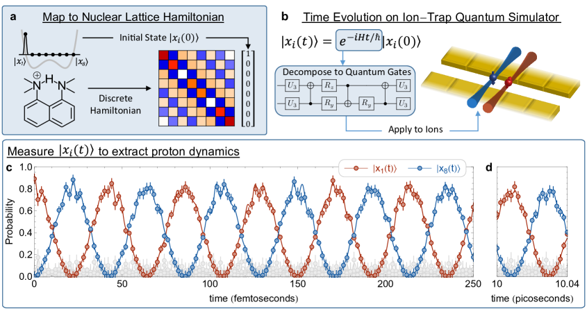
Figure 1: Coherent dynamics of a shared-proton wavepacket. (a) The quantum dynamics of a short-strong hydrogen bonded system are mapped onto a discrete basis. Each basis state represents a shared-proton wavepacket occupying one of the equally-spaced lattice sites between the donor/acceptor frameworks. The discrete Hamiltonian is formed from writing the kinetic and potential energy operators for the shared-proton in this system. (b) Time evolution under the nuclear Hamiltonian is achieved by applying a unitary propagator to an initial wavepacket state. The unitary operator is decomposed into single- and two-qubit quantum gates which are applied to a trapped-ion quantum computer. (c) The quantum dynamics of the trapped-ion system emulate those of the shared proton wavepacket. When a wavepacket is initialized near the left side of the anharmonic potential well, its dynamics are found to oscillate coherently between the donor and acceptor groups. Solid lines show the exact numerical solution to the Schrödinger equation including decoherence effects. (d) Our trapped-ion experiment remains coherent for many hundreds of emulated shared-proton oscillations with no visible reduction in contrast.

III Wavepacket Dynamics on Ion-Trap Systems

To emulate the chemical dynamics of this hydrogen-bonded system, lasers are used to prepare and manipulate the internal electronic states of trapped atomic ions (Fig. 1b). Qubit levels are encoded in the ²S${}_{1/2}\ket{F=0,m_{F}=0}$ and $\ket{F=1,m_{F}=0}$ hyperfine ‘clock’ states of ¹⁷¹Yb⁺ ions, denoted $\ket{0}$ and $\ket{1}$, respectively Olmschenk et al. (2007). State preparation proceeds by optically pumping all qubits to $\ket{0}$, then performing local rotations to generate a state corresponding to an initial shared-proton wavepacket. To find the shared-proton wavepacket at a later time $t$, we time-evolve the initial state under the unitary propagator $U(t)=e^{-iHt/\hbar}$, where $H$ is the ion-trap Hamiltonian that encodes the effective nuclear dynamics. While $H$ is generically expressed in terms of Ising-type XX and YY interactions Saha et al. (2021a), here we exploit the small system size to optimally decompose the propagator $U(t)=e^{-iHt/\hbar}$ into a sequence of seven single-qubit rotations (with time-dependent angles) and three controlled-NOT (CNOT) gates Vatan and Williams (2004); Tucci (2005); Maslov (2017); Mølmer and Sørensen (1999).

We generate single- and two-qubit gates by applying spin-dependent optical dipole forces to ions confined in a surface-electrode trap (Sandia HOA-2.1 Maunz (2016)). Each ion is addressed by two laser beams near 355 nm: one tightly-focused individual-addressing beam and one global beam that targets all ions simultaneously. The beams are arranged such that their wavevector difference $\Delta\vec{k}$ lies along the transverse principal axes in plane with the trap surface. The two beams contain frequency components whose difference can be matched to the resonant transition of the ion qubit at $\nu_{0}=12.642819$ GHz to drive single-qubit gates, or detuned symmetrically from $\nu_{0}$ to drive Mølmer-Sørensen two-qubit interactions. Gate times for single-qubit $\pi/2$ flips are typically 10 $\mu$s with $99.5\%$ fidelity, while typical Mølmer-Sørensen gates require 200 $\mu$s for full entanglement and a typical $97\%$ fidelity.

After initializing the ion qubits and applying gates to simulate Hamiltonian evolution for time $t$, the qubit states are measured to determine the time-evolved shape of the shared-proton wavepacket. At each timestep, measurements of the trapped-ion qubit states determine the probability of finding the shared-proton on each of the $2^{N}$ lattice sites. Detection of the final ion states is accomplished by capturing their spin-dependent fluorescence into a fiber array, where each fiber is coupled to an individual photomultiplier-tube (PMT). Site-resolved detection allows for discrimination of each qubit’s logical $\ket{0}$ or $\ket{1}$ states with $99.0\%$ detection fidelity as well as the probability overlap with all possible basis states. Experiments are repeated 1000 times at each timestep to limit the statistical error contributions from quantum projection noise. The time-dependent proton dynamics are then determined by mapping the observed ion dynamics back to the discrete proton basis sm .

In Figure 1c, we highlight the probabilities of finding the shared-proton on the left-most ($\ket{x_{1}}$) and right-most ($\ket{x_{8}}$) lattice sites on the potential energy surface, when it is initialized in the $\ket{x_{1}}$ position. For this initial state, the shared-proton wavepacket is found to exhibit large-amplitude, coherent oscillations between the donor/acceptor groups as well as smaller-amplitude, higher-frequency oscillations; intermediate lattice sites contribute negligibly to the dynamics in this case (grey points in Fig. 1c). We emphasize that the solid lines in Fig. 1c are not fits to the data; rather, they are an exact numerical solution to the Schrödinger equation in the presence of known quantum gate infidelities.

In our experiments, the quantum circuit in Fig. 1b is implemented with a $\sim 90\%$ fidelity for any simulated evolution time $t$. This results in effective shared-proton oscillations that remain coherent for arbitrarily long times with no apparent decrease in contrast. Figure 1d shows a continuation of the dynamics from Fig. 1c, hundreds of oscillation periods after the wavepacket is initialized. Remarkably, since the gate errors are the same for each timestep, they do not affect the frequency information encoded in the time dynamics. For instance, we show below that the shared-proton vibrational frequencies may be determined to $>99.9\%$ accuracy despite the $\sim 90\%$ overall circuit fidelity.

Initializing our system in different quantum states, which corresponds to initializing the shared-proton wavepacket on different lattice sites, leads to a variety of different time-dependent oscillations. In Figure 2a, the effective shared-proton state is initialized to occupy the left-most lattice site at $t=0$. Just as in Fig. 1c-d, the time dynamics reveal wavepacket jumps between the $\ket{x_{1}}$ and $\ket{x_{8}}$ lattice sites at a rate of $\approx$24 THz (800 cm^-1). In contrast, when the shared-proton state is initialized on the second lattice site (Fig. 2b), a continuous oscillation between sites $\ket{x_{2}}$ through $\ket{x_{7}}$ is observed with nearly-zero probability of occupying the extrema ($\ket{x_{1}}$ and $\ket{x_{8}}$). When positive and negative wavepacket components are introduced in the left- and right- wells (respectively), as in Fig. 2c, strong oscillations are observed along with destructive interference effects near the center of the double well potential. Finally, when the initial proton wavepacket is prepared in an eigenstate of the nuclear Hamiltonian (Fig. 2d), no time-dependent dynamics are expected nor observed.

Figure 2: Experimentally-determined dynamics of a shared-proton in DMANH⁺. The observed time evolution depends on whether the shared-proton wavepacket is initialized (a) near the donor site; (b) near one of the potential energy surface minima; (c) split between the two minima with opposite phase; or (d) in an eigenstate of the double-well potential. Oscillations in both space and time are observed in all cases, except in (d), where the system remains in its eigenstate.

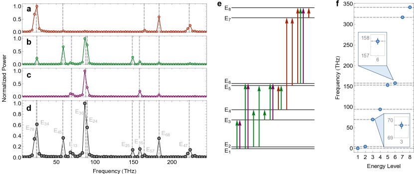
Figure 3: Experimentally-determined frequency and energy spectra of a shared-proton in DMANH⁺. (a)-(c) The time evolution data for the initial states in Fig. 2a-c are Fourier-transformed to reveal frequency spectra of the shared-proton oscillation. Each peak corresponds to a frequency splitting between eigenstates of the discrete nuclear Hamiltonian. (d) The data in a-c are summed to produce a final frequency spectrum. Dashed grey lines and labels show predicted frequencies from exact diagonalization of the nuclear Hamiltonian. (e) The extracted frequencies from a-d, color-coded by their parent spectrum, allow the relative energies of all eigenstates to be experimentally determined. (f) The quantum-computed energy eigenstates of the nuclear Hamiltonian (blue dots) are compared to the exact-diagonalization result (dashed grey lines). Typical error bars (1 s.d.) are shown in the insets.

IV Determination of Vibrational Spectra from Wavepacket Dynamics

Our emulation of the shared-proton wavepacket dynamics enables a high-accuracy determination of its vibrational frequencies. Consider the nuclear Hamiltonian $H$, which has eigenstates $\phi_{i}(x)$ and energy eigenvalues $E_{i}$. Any chosen initial state $\chi(x,0)$ may be written in terms of this eigenstate basis, with corresponding time evolution:

$$\chi(x,t)=\sum_{i}c_{i}(0)e^{-iE_{i}t/\hbar}\phi_{i}(x)$$ (8)

Hence, the probability of finding the shared proton at position $x$ at time $t$ is given by

$$|\chi(x,t)|^{2}=\sum_{i,j}c_{j}^{*}(0)c_{i}(0)e^{i(E_{j}-E_{i})t/\hbar}\phi_{j}^{*}(x)\phi_{i}(x)$$ (9)

The time evolution of any initial state therefore is comprised of oscillations at all possible frequency differences between all pairs of energy eigenstates. For each frequency component, the strength is governed by the product of overlap amplitudes $c_{j}^{*}(0)c_{i}(0)$, that is, the coefficients comprising the initial wavepacket.

To extract the oscillation frequencies of the shared-proton wavepacket in our hydrogen-bonded system, we perform a Fourier transform of the measured time-evolution data presented in Figure 2. Mathematically, this operation is equivalent to taking

$$\begin{split}\int e^{i\omega t}&|\chi(x,t)|^{2}dt=\\ &\sum_{i,j}\left[\int e^{i\omega t}e^{i(E_{j}-E_{i})t/\hbar}dt\right]c_{j}^{*}c_{i}\phi_{j}^{*}(x)\phi_{i}(x)\\ =&\sum_{i,j}\delta(\omega-(E_{j}-E_{i})/\hbar)c_{j}^{*}c_{i}\phi_{j}^{*}(x)\phi_{i}(x)\\ \end{split}$$ (10)

which produces peaks in the Fourier spectrum corresponding to frequency differences between energy eigenstates, $(E_{j}-E_{i})/\hbar$. This expression is also related to the Fourier transform of the density matrix auto-correlation function, ${\text{Tr}}[\rho(0)\rho(t)]$ sm .

Fourier-transforms of the shared-proton time dynamics (Fig. 2a-c) are shown in Fig. 3a-c, along with a cumulative spectrum in Fig. 3d. The extracted peaks provide a direct measurement of the energy eigenstate differences $E_{ij}\equiv(E_{j}-E_{i})$, which show excellent agreement with the frequencies predicted from exact diagonalization of the nuclear Hamiltonian (grey dashed lines in Fig. 3a-d). Note that since the initial wavepacket state in Figure 2d was prepared in an eigenstate and contains minimal time dynamics, its Fourier transform contains no meaningful frequency information.

Using the measured energy differences $E_{ij}$ in Fig. 3a-d, we experimentally reconstruct the full energy eigenspectrum of our nuclear Hamiltonian. Since the shared-proton basis has been discretized onto 8 lattice sites, our Hamiltonian contains 8 energy eigenvalues which are calculable and drawn to scale in Fig. 3e. The set of measurements $\{E_{ij}\}$ from Fig. 3a-d provides more information than necessary to determine the relative spacings of all energy levels. This overcompleteness arises from our multiple different wavepacket initializations, and it allows for multiple independent measurements of specific energy splittings and reduced error in our final results.

The vibrational energies obtained directly from the ions’ time dynamics are compared in Fig. 3f to the exact diagonalization results (dashed grey lines). Exceptional agreement is found in all cases. Typical measurement uncertainties are at the level of $0.1\%$, which corresponds to 3.3 cm^-1 wavenumbers and is well within the range of spectroscopic accuracy for such molecular vibration problems.

V Extension to Multiple Nuclear Degrees of Freedom

The implementation of multi-dimensional molecular dynamics studies on quantum hardware is complicated by multiple factors. Molecules contain many correlated nuclear degrees of freedom, and each of these correlated nuclear degrees of freedom needs to be represented in some discretized basis. For ${\cal N}$ discretizations (or basis vectors) per nuclear degree of freedom and $N$ nuclear degrees of freedom, the complexity of information grows approximately as ${\cal N}^{N}$. As a result, quantum nuclear dynamics is thought to be an exponentially hard problem. In general, the Hamiltonian for such a system may be written as

$${\cal{H}}(\mathbf{\bar{x}},\mathbf{\bar{x}}^{\prime}) ={\cal K}(x_{1},x_{1}^{\prime})\otimes{\cal I}(x_{2},x_{2}^{\prime})\otimes\cdots\otimes{\cal I}(x_{N},x_{N}^{\prime})$$

$$+\sum_{i=2}^{N-1}{\cal I}(x_{1},x_{1}^{\prime})\otimes\cdots\otimes{\cal I}(x_{i-1},x_{i-1}^{\prime})\otimes$$

$$\phantom{+}{\cal K}(x_{i},x_{i}^{\prime})\otimes{\cal I}(x_{i+1},x_{i+1}^{\prime})\otimes\cdots\otimes{\cal I}(x_{N},x_{N}^{\prime})$$

$$+{\cal I}(x_{1},x_{1}^{\prime})\otimes\cdots\otimes{\cal I}(x_{N-1},x_{N-1}^{\prime})\otimes{\cal K}(x_{N},x_{N}^{\prime})$$

$$+{\cal V}(\mathbf{\bar{x}},\mathbf{\bar{x}}^{\prime})$$ (11)

where $\mathbf{\bar{x}}\equiv\quantity{x_{1},x_{2},\ldots,x_{N}}$. While the kinetic energy part of the Hamiltonian, $\left\{{\cal K}(x_{i},x_{i}^{\prime})\right\}$, is decoupled across all degrees of freedom and for each dimension is represented using Eq. (1), the potential energy surface correlates these dimensions and drives the computational complexity of the problem. Additionally, for quantum nuclear dynamics the term ${\cal V}(\mathbf{\bar{x}},\mathbf{\bar{x}}^{\prime})$ is determined by the properties of electrons; when accurate electron correlation methods are employed, the computational cost for each electronic structure calculation may grow in a steeply algebraic manner. Furthermore, the number of terms needed to determine ${\cal V}(\mathbf{\bar{x}},\mathbf{\bar{x}}^{\prime})$ may scale in the worst case as ${\cal N}^{N}$ thus rendering the quantum molecular dynamics problem, in conjunction with determination of the electronic potential energy surface, to be computationally intractable for large systems. This severely restricts the study of many problems at the forefront of biological, materials and atmospheric systems.

For the process of quantum propagation, where either a quantum circuit is to be generated based on the time-evolution operator constructed from Eq. (11), or a controllable Ising-type quantum system is created that may be used to simulate the system depicted by Eq. (11), the very act of processing Eq. (11) requires, at the worst case, exponential resources. This can already be seen for the one-dimensional dynamics in DMANH⁺: any oscillations in the N–N length will affect the nature of the double well potential that confines the shared hydrogen nucleus, requiring multiple iterative calculations to predict the spectroscopic behavior of the system.

Figure 4: Tensor network diagram of the MPS representation of the wave function $\chi(\mathbf{\bar{x}};t)$. (See Eq. (12).) In the discrete position basis, the $N$-dimensional wave function is pictured as an $N$-order tensor, which is factorized as a product of order-2 and order-3 tensors $\phi^{[k]}$.

Here we present a theoretical formalism for multi-dimensional quantum nuclear dynamics, the critical role played by the current experimental results, and the potential quantum advantage enabled by this framework. We begin by writing a general multi-dimensional quantum nuclear wavefunction as a tensor network. Specifically, in our case, we illustrate this by writing the wavefunction as a matrix product state (MPS) Östlund and Rommer (1995); Fannes et al. (1992, 1994); Affleck et al. (1987, 1988); Vidal (2003); Schollwöck (2011):

$$\chi(\mathbf{\bar{x}};t)=\sum_{\bar{\bm{\alpha}}}^{\bar{\bm{\eta}}}\tensor{*}{\phi}{{}^{[1]}{}^{x_{1}}_{\alpha_{1}}}\quantity[\prod_{j=2}^{N\text{-}1}\tensor{*}{\phi}{{}^{[j]}{}^{x_{j}}_{\alpha_{j\text{-}1}}{}_{\alpha_{j}}}]\tensor{*}{\phi}{{}^{[N]}{}^{x_{N}}_{\alpha_{N\text{-}1}}}.$$ (12)

In other words, on the l.h.s. of Eq. 12, the $N$-dimensional wavefunction $\chi(\mathbf{\bar{x}};t)$ is thought of as an order-$N$ tensor which is factorized into a product of order-2 and order-3 tensors $\phi^{[j]}$, each corresponding to one-dimensional functions of the coordinate $x_{j}$. The sum runs through the so-called entanglement variables $\bar{\bm{\alpha}}\equiv\quantity{\alpha_{1},\alpha_{2},\ldots,\alpha_{N-1}}$ with respective limits $\bar{\bm{\eta}}\equiv\quantity{\eta_{1},\eta_{2},\ldots,\eta_{N-1}}$, commonly named entanglement dimension, bond dimension, or Schmidt rank. Equation (12) is graphically illustrated as a tensor network diagram in Figure 4. Using tensor networks, the time evolution operator for the Hamiltonian in Eq. (11) may also be written Schollwöck (2011); Verstraete et al. (2004); Pirvu et al. (2010) as a tensor network operator:

$${\cal{U}}(\mathbf{\bar{x}},\mathbf{\bar{x}}^{\prime};t)=\sum_{\bar{\bm{\beta}}}\tensor{*}{{\cal{U}}}{{}^{[1]}{}^{t;x_{1},x_{1}^{\prime}}_{\beta_{1}}}\quantity[\prod_{j=2}^{N\text{-}1}\tensor{*}{{\cal{U}}}{{}^{[j]}{}^{t;x_{j},x_{j}^{\prime}}_{\beta_{j\text{-}1}}{}_{\beta_{j}}}]\tensor{*}{{\cal{U}}}{{}^{[N]}{}^{t;x_{N},x_{N}^{\prime}}_{\beta_{N\text{-}1}}},$$ (13)

where the degree of entanglement captured within the time-evolution, designated by the parameter $\bar{\bm{\beta}}$ is evidently different from that in Eq. (12) and pertains to the physics captured within the Hamiltonian (and in fact ${\cal V}$ in Eq. (11)) used to create such a time-evolution operator. Thus, we may equivalently write

$${\cal{V}}(\mathbf{\bar{x}},\mathbf{\bar{x}}^{\prime})=\delta_{\mathbf{\bar{x}},\mathbf{\bar{x}}^{\prime}}\sum_{\bar{\bm{\beta}}}\tensor{*}{{\cal{V}}}{{}^{[1]}{}^{x_{1},x_{1}^{\prime}}_{\beta_{1}}}\quantity[\prod_{j=2}^{N\text{-}1}\tensor{*}{{\cal{V}}}{{}^{[j]}{}^{x_{j},x_{j}^{\prime}}_{\beta_{j\text{-}1}}{}_{\beta_{j}}}]\tensor{*}{{\cal{V}}}{{}^{[N]}{}^{x_{N},x_{N}^{\prime}}_{\beta_{N\text{-}1}}},$$ (14)

where it is assumed that the potential is diagonal in the coordinate representation $\ket{\bar{x}}$ used here. Equation (13) yields the critical feature that each dimension can be independently propagated, on different quantum systems, and this aspect is pictorially represented using the purple and green edges in Figure 5. In other words, Figure 5 depicts the full multi-dimensional time-evolution process as,

$$\chi(\mathbf{\bar{x}};t)= \int d\mathbf{\bar{x}}^{\prime}\;{\cal{U}}(\mathbf{\bar{x}},\mathbf{\bar{x}}^{\prime};t)\;\chi(\mathbf{\bar{x}}^{\prime};t=0)$$

$$= \sum_{\bar{\bm{\alpha}}}\sum_{\bar{\bm{\beta}}}\left[\int dx_{1}^{\prime}\tensor{*}{{\cal{U}}}{{}^{[1]}{}^{t;x_{1},x_{1}^{\prime}}_{\beta_{1}}}\tensor{*}{\phi}{{}^{[1]}{}^{x_{1}^{\prime}}_{\alpha_{1}}}\right]$$

$$\phantom{\sum_{\bar{\bm{\alpha}}}\sum_{\bar{\bm{\beta}}}}\quantity[\prod_{j=2}^{N\text{-}1}\int dx_{j}^{\prime}\tensor{*}{{\cal{U}}}{{}^{[j]}{}^{t;x_{j},x_{j}^{\prime}}_{\beta_{j\text{-}1}}{}_{\beta_{j}}}\tensor{*}{\phi}{{}^{[j]}{}^{x_{j}^{\prime}}_{\alpha_{j\text{-}1}}{}_{\alpha_{j}}}]$$

$$\phantom{\sum_{\bar{\bm{\alpha}}}\sum_{\bar{\bm{\beta}}}}\left[\int dx_{N}^{\prime}\tensor{*}{{\cal{U}}}{{}^{[N]}{}^{t;x_{N},x_{N}^{\prime}}_{\beta_{N\text{-}1}}}\tensor{*}{\phi}{{}^{[N]}{}^{x_{N}^{\prime}}_{\alpha_{N\text{-}1}}}\right]$$

$$= \sum_{\bar{\bm{\alpha}},\bar{\bm{\beta}}}\tensor{*}{\phi}{{}^{[1]}{}^{t;x_{1}}_{\beta_{1}\alpha_{1}}}\quantity[\prod_{j=2}^{N\text{-}1}\tensor{*}{\phi}{{}^{[j]}{}^{t;x_{j}}_{\beta_{j\text{-}1}}{}_{\beta_{j}}{}_{\alpha_{j\text{-}1}}{}_{\alpha_{j}}}]\tensor{*}{\phi}{{}^{[N]}{}^{t;x_{N}}_{\beta_{N\text{-}1}}{}_{\alpha_{N\text{-}1}}}.$$ (15)

Figure 5: Action of the time evolution operator $\mathcal{U}(\mathbf{\bar{x}},\mathbf{\bar{x}^{\prime}};t)$ onto the MPS wave function $\chi(\mathbf{\bar{x}};t=0)$ shown in Eq. (15).

where the time evolution for each component, for example, depicted by the purple and green edges in Figure 5:

$$\tensor{*}{\phi}{{}^{[j]}{}^{t;x_{j}}_{\beta_{j\text{-}1}}{}_{\beta_{j}}{}_{\alpha_{j\text{-}1}}{}_{\alpha_{j}}}\equiv\int dx_{j}^{\prime}\,\tensor{*}{{\cal{U}}}{{}^{[j]}{}^{t;x_{j},x_{j}^{\prime}}_{\beta_{j\text{-}1}}{}_{\beta_{j}}}\tensor{*}{\phi}{{}^{[j]}{}^{x_{j}^{\prime}}_{\alpha_{j\text{-}1}}{}_{\alpha_{j}}}$$ (16)

may be carried out on separate quantum simulators. Equation (15) is completely represented in Figure 5. The top row here is the MPS state in Eq. (12), as evidenced through comparison with Figure 4. The second row (green) represents the propagator in Eq. (14) with entanglement dimensions $\bar{\bm{\beta}}$; the connected green and purple lines indicate the integration over the primed variables in Eqs. (15) and (16). As noted, each such integration (or time-evolution) may be mapped on to a separate quantum system or quantum processor. Finally the bottom (blue) row of Figure 4 shows the right side of Eq. (15) where the entanglement variables are now double indexed as $\bar{\bm{\alpha}},\bar{\bm{\beta}}$.

Given the structure and sparsity of the system Hamiltonian, it is critical to assess the number of parameters in the unitary evolution depicted by Eqs. (13) and (14) since these will eventually determine the nature of the quantum circuit, the associated depth, and complexity. At the outset, let us emphasize that the number of parameters within the direct unitary evolution of Eq. (11) could be as many as ${\cal O}\left({\cal N}^{N}\right)$, as already noted above. This implies that, when using $n$ qubits per nuclear dimension, the number of parameters in Eq. (11) is $2^{nN}$ in the worst case.

However, when Eqs. (13) and (14) are used for quantum propagation, one only needs of the order of $\left({\cal N}*N\right)$, or $2^{n}N$ parameters inside the same set of $n*N$ qubit quantum system. This is because, for most chemical systems the number of product vectors in Eq. (14) is expected to be small number as compared to the total number of nuclear basis functions, ${\cal N}^{N}$. This result appears from the “area law of entanglement entropy” Orús (2014), where it is thought to be the case that the extent of entanglement in most physical systems, as depicted by the number of product functions in Eq. (14), scales as the area, rather than the volume of the Hilbert space. In other words, the number of non-zero terms in Eq. (14) is of order $\left({\cal N}*N\right)$ times the number of terms in the summation in Eq. (14). This last part is expected to be small compared to both ${\cal N}$ and $N$, for large enough values of both parameters, based on the area law of entanglement entropy. This is a major advantage for the current formalism, and future experimental implementations will actively probe the limits of this apparent theoretical quantum advantage that promises an exponential circuit depth reduction of the order of $2^{nN}/(2^{n}N)$.

Thus, the tensor network formalism allows the overall unitary propagator to be factorized into separate pieces shown as the green blocks in Figure 5; the action of each of which may be constructed in parallel as is seen from the above equations. This critical feature when combined with the one-dimensional propagation algorithm presented here and in Ref. Saha et al., 2021a, yields a general approach to treat the classically intractable multi-dimensional quantum nuclear dynamics problem on a family of quantum systems.

VI Conclusions

This paper has presented a rigorous theoretical framework and experimental demonstration for treating general chemical dynamics problems using quantum hardware. We have shown how molecular systems with anharmonic potential energy landscapes – such as the ubiquitous hydrogen bond – may be mapped to a system of controllable interacting quantum bits. We have performed a proof-of-principle demonstration of our mapping, finding excellent agreement between the observed hydrogen-bond dynamics and extracted spectra compared with those calculated on classical hardware. Finally, we discussed an outlook towards extending our approach to more complex chemical systems with multiple correlated nuclear degrees of freedom.

We remark that our experimental technique for extracting all energy eigenvalues of a many-body Hamiltonian has yielded higher accuracies (by nearly two orders-of-magnitude) than previous efforts using trapped-ion quantum systems Senko et al. (2014); Jurcevic et al. (2015). We note that this high accuracy is driven by the resilience of frequency information in our time-series data, despite accumulated quantum gate errors at the $\sim 10\%$ level. Our observations establish that current-generation, noisy quantum hardware can already serve as a precise computational resource for studying the spectral features of many-body Hamiltonians.

We have, for the first time, demonstrated that generalized nuclear dynamics can be modeled exactly using a qubit-based quantum processor. This is a marked departure from existing literature, where vibrations within the harmonic approximation are mapped to Bosonic systems. Building on the high-accuracy quantum simulations presented here, we will broaden our implementation to include multiple correlated nuclear degrees of freedom within the nuclear Hamiltonian to capture more realistic wavepacket trajectories across the potential energy surface and also allow for Boltzmann averaging over thermally-fluctuating donor-acceptor distances. Ultimately, we expect to compare and validate our quantum-computed results with experiments performing gas-phase spectroscopy, for which the Hamiltonian description of an isolated nuclear wavepacket is most appropriate.

VII Acknowledgements

The work of P.R., D.S., M.A.L-R., A.D., J.M.S., A.S., and S.S.I are supported by the U.S. National Science Foundation under award OMA-1936353. The QSCOUT open-access testbed is funded by the U.S. Department of Energy, Office of Science, Office of Advanced Scientific Computing Research Quantum Testbed Program. Sandia National Laboratories is a multimission laboratory managed and operated by National Technology & Engineering Solutions of Sandia, LLC, a wholly owned subsidiary of Honeywell International Inc., for the U.S. Department of Energy’s National Nuclear Security Administration under contract DE-NA0003525. This paper describes objective technical results and analysis. Any subjective views or opinions that might be expressed in the paper do not necessarily represent the views of the U.S. Department of Energy or the United States Government.

Supplementary Material for
“Quantum Computation of Hydrogen Bond Dynamics and Vibrational Spectra”
 

Supplementary Material for
“Quantum Computation of Hydrogen Bond Dynamics and Vibrational Spectra”

DMANH⁺ Molecule – The specific intra-molecular proton transfer problem considered here is that in the protonated 1,8-bis(dimethylamino)naphthalene (DMANH⁺) system. The DMAN molecule has an extremely large proton affinity of $242$ kcal/mol Lias et al. (1984), with DMANH⁺ $pK_{a}$ value in the range $12.1-12.3$ Perrin (1972). The NHN⁺ hydrogen bond in DMANH⁺ has been frequently studied as a model for short, low-barrier hydrogen bonds that have a role in certain enzyme-catalyzed reactions Perrin and Nielson (1997); Cleland and Kreevoy (1994). In solution, the shared proton delocalization in DMANH⁺ is controlled by a low-barrier symmetric double-well potential, with barrier height being influenced by solvent and temperature Perrin (2010); Pietrzak et al. (2010). In this publication, the shared proton reduced dimensional potential for the most significant donor-acceptor distance, that is N-N distance equal to 2.53 Å, is used to perform quantum dynamics studies on an ion-lattice quantum computer. We treat the shared proton stretch dimension within the Born-Oppenheimer limit. The nuclear Hamiltonian is determined by the ground electronic state potential energy surface.

Quantum Computation using the QSCOUT ion-trap device – The experiment described here was performed on the room temperature Quantum Scientific Computing Open User Testbed (QSCOUT) system Clark et al. (2021). In this work, we used two ¹⁷¹Yb⁺ ions trapped $70~{}\mu$m off the surface of an HOA-2.1 trap Maunz (2016) with radial secular frequencies , $\nicefrac{{\omega}}{{2\pi}}$, of 2.0 MHz and 2.4 MHz. The axial frequency is set to match our individual addressing and imaging fiber spacing of about $4.5~{}\mu$m. As previously mentioned, the ions are manipulated between the ²S${}_{1/2}\ket{F=0,m_{F}=0}$ and $\ket{F=1,m_{F}=0}$ hyperfine states, denoted $\ket{0}$ and $\ket{1}$, respectively Olmschenk et al. (2007). We use Doppler cooling and resolved sideband cooling to cool the ions to near the ground state then prepare them in the $\ket{0}$ state using optical pumping.

The coherent operations are performed using two counterpropagating 355 nm Raman beams from a single laser. These drive a two-photon transition Wineland et al. (1998); Leibfried et al. (2003) via a virtual state, 33 THz detuned from the ²P_1/2 level. The global beam has an elliptical $1/e^{2}$ beam waist of $10.9~{}\mu$m vertically and $182.8~{}\mu$m horizontally, such that scattering off the surface is minimized but the ions are illuminated with near uniform intensity. The individual addressing beams are created using a 32-channel acousto-optic modulator (AOM) with integrated optics L3 Harris (2020) for creating 32 parallel and individually controllable beams. We use custom optics to create an elliptical profile at the ion from each of these beams with a vertical waist of $8~{}\mu$m, also to minimize scatter off the surface, and a horizontal beam waist of $0.8~{}\mu$m to achieve a $4.5~{}\mu$m ion spacing.

The Jaqal code that defines the gate sequences and rotation angles is fed directly into the experimental machine. This work used a combination of single qubit gates and two qubit CNOT gates. The single qubit rotations, $R(\theta,\phi)$, where $\theta$ is the rotation angle and $\phi$ is the phase defined in the Jaqal code, are generated using only the individual addressing beam in co-propagating configuration by applying both Raman tones. The $R_{z}$ gate is performed in software using a phase advance. The single qubit gate times are approximately $15~{}\mu$s and single qubit gate fidelities are about 99.5(3)%.

The CNOT gate is a Mølmer-Sørensen (MS) interaction between a series of single qubit rotations. We perform the MS gate by applying two frequency tones on the individual addressing beam corresponding to each ion and a single frequency tone on the global beam. The combination of the frequencies results in a pulse capable of driving the MS interaction. MS gate times are approximately $200~{}\mu$s and fidelities are 97(1)%. We create a CNOT gate using an MS gate with a series of single qubit wrapper gates which give a combined CNOT gate fidelity of 96.5(1.5)%.

We use a high numerical aperture imaging system to reduce the detection time and increase readout fidelity Noek et al. (2013). The collected light is coupled into a multimode fiber array, such that each ion location is aligned to a different fiber Clark et al. (2021). Each fiber is connected to a dedicated photomultiplier tube for counting the photons, thus allowing for simultaneous and distinguishable detection between the two ions. An elliptical $370~{}$nm laser beam that is resonant to the ²S${}_{1/2}\ket{F=1,m_{F}=0}\rightarrow^{2}$P${}_{1/2}\ket{F=0,m_{F}=0}$ transition illuminates both ions with comparable intensity. We apply the resonant light for $350~{}\mu$s, ions in state $\ket{1}$ are detected as bright with 99(0.3)% fidelity.

Mapping from Ion Trap to Molecule – After allowing for time evolution in each of the sub-blocks and detecting the ion qubit states, the measurement outcomes from the ion-trap system must be re-mapped back to the proton grid basis. For specificity in this section, we will focus on the mapping to the first proton lattice site $\ket{x_{1}}$; the re-mapping to all other lattice sites follows an identical procedure.

From the map definition in Eq. 5 of the main text, the probability amplitude $c_{1}$ for the shared-proton wavepacket on lattice site $\ket{x_{1}}$ is given by

$$c_{1}=\frac{1}{\sqrt{2}}(c_{\tilde{1}}+c_{\tilde{8}})$$ (17)

where the $c_{\tilde{n}}$ indicate probability amplitudes in the ion-trap basis (see Eqs. 5-6 in the main text). The overall lattice site probability $P(\ket{x_{1}})$ is then

$$P(\ket{x_{1}}) =|c_{1}|^{2}=\frac{1}{2}(|c_{\tilde{1}}|^{2}+|c_{\tilde{8}}|^{2}+2\text{Re}[c_{\tilde{1}}^{*}c_{\tilde{8}}])$$ (18)

$$=\frac{1}{2}(P(\ket{\tilde{1}})+P(\ket{\tilde{8}})+2\text{Re}[c_{\tilde{1}}^{*}c_{\tilde{8}}])$$ (19)

where $P(\ket{\tilde{1}})$ and $P(\ket{\tilde{8}})$ are the probabilities of measuring the first state in the upper sub-block, and the last state in the lower sub-block, respectively.

To map the cross-term, we write the complex probability amplitude $c_{\tilde{n}}=A_{\tilde{n}}e^{i\phi_{\tilde{n}}}=\sqrt{P(\ket{\tilde{n}})}e^{i\phi_{\tilde{n}}}$, such that

$$\text{Re}[c_{\tilde{1}}^{*}c_{\tilde{8}}]=\sqrt{P(\ket{\tilde{1}})P(\ket{\tilde{8}})}\cos(\phi_{\tilde{8}}-\phi_{\tilde{1}})$$ (20)

Finally, using that the phase accrued at time $t$ can be written to first order as $\phi_{\tilde{n}}=\tilde{\mathcal{H}}^{Mol}_{nn}t/\hbar$, the full shared-proton probability (Eq. 18) may be constructed using only ion-trap measurement probabilities and the original molecular Hamiltonian.

Vibrational Spectra from time-correlation functions – We examine our quantum circuit based dynamics algorithm by simulating the reduced dimensional shared proton vibrational dynamics in the 1,8-bis(dimethylamino) naphthalene (DMANH⁺) molecular system on an ion-trap quantum computing system. We compare our results with results from classical simulation of the quantum dynamics. As a result, for the first time, we present, in this paper, vibrational properties determined from quantum computing experiments. The approach used to achieve this is as follows.

The time-dependent density matrix in an eigenstate representation is given by,

$$\rho(t) = \ket{\chi(t)}\bra{\chi(t)}=e^{-\imath{\cal H}t/\hbar}\ket{\chi(0)}\bra{\chi(0)}e^{\imath{\cal H}t/{\hbar}}$$ (21)

$$= \sum_{i,j}c_{i}(0)c_{j}^{*}(0)e^{-\imath{\cal H}t/{\hbar}}\ket{\phi_{i}}\bra{\phi_{j}}e^{\imath{\cal H}t/{\hbar}}$$

$$= \sum_{i,j}c_{i}(0)c_{j}^{*}(0)e^{\imath(E_{i}-E_{j})t/{\hbar}}\ket{\phi_{i}}\bra{\phi_{j}},$$

and is used to construct the Fourier transform of the density-density time auto-correlation function, ${\text{Tr}}[\rho(0)\rho(t)]$ as

$$\int_{-\infty}^{+\infty}dte^{{\imath\omega t}}\;{\text{Tr}}[\rho(0)\rho(t)] = \int_{-\infty}^{+\infty}dte^{{\imath\omega t}}\;{\text{Tr}}\left[\ket{\chi(0)}\bra{\chi(0)}\sum_{i,j}c_{i}(0)c_{j}^{*}(0)e^{\imath(E_{i}-E_{j})t/{\hbar}}\ket{\phi_{i}}\bra{\phi_{j}}\right]$$ (22)

$$= \sum_{i,j}|c_{i}(0)|^{2}|c_{j}(0)|^{2}\;\delta\left(\omega-(E_{i}-E_{j})/\hbar\right)$$

which yields the difference in eigenenergies, weighted by contributions from the initial state, much like a standard experimental result. Equation 10 in the main text has a similar form as Eq. 22 and also depends on the difference in eigenenergies, but differs in intensities. To gauge the relation between the intensities in Eqs. (10) and (22), one may rewrite Eq. (22) using the convolution theorem Press et al. (1992) as

$$\int dxdx^{\prime}\int_{-\infty}^{+\infty}dtdt^{\prime}e^{{\imath\omega(t-t^{\prime})}}\;\rho(x;x^{\prime};t)\rho(x,x^{\prime};t^{\prime})=$$

$$\phantom{\int dxdx^{\prime}}\int dxdx^{\prime}{\left\{\left|\int_{-\infty}^{+\infty}dte^{{\imath\omega t}}\;\rho(x;x^{\prime};t)\right|\right\}}^{2}$$ (23)

Equation 10 in the main text is simply the diagonal ($x=x^{\prime}$) portion of the term inside curly brackets $\left\{\cdots\right\}$ on the rights side of Eq. (23). For example, the right side of Eq. (23) may be written as

$$\int dx{\left|\int_{-\infty}^{+\infty}dte^{{\imath\omega t}}\;\rho(x;x;t)\right|}^{2}+$$

$$\int_{x\neq x^{\prime}}dxdx^{\prime}{\left|\int_{-\infty}^{+\infty}dte^{{\imath\omega t}}\;\rho(x;x^{\prime};t)\right|}^{2}$$ (24)

and using Eq. (21), further reduced to,

$$\int dx{\left\{\left|\int_{-\infty}^{+\infty}dte^{{\imath\omega t}}\;\sum_{i,j}c_{i}(0)c_{j}^{*}(0)e^{\imath(E_{i}-E_{j})t/{\hbar}}{\phi_{i}(x)}{\phi_{j}(x)}\right|\right\}}^{2}+$$

$$\int_{x\neq x^{\prime}}dxdx^{\prime}\left|\int_{-\infty}^{+\infty}dte^{{\imath\omega t}}\sum_{i,j}c_{i}(0)c_{j}^{*}(0)e^{\imath(E_{i}-E_{j})t/{\hbar}}{\phi_{i}(x)}{\phi_{j}(x^{\prime})}\right|^{2}$$ (25)

Note that the term inside curly brackets $\left\{\cdots\right\}$ on the first line of Eq. (25) is identical to the left side of Eq. 10 in the main text. Thus by measuring Eq. 10, we have a direct gauge on the standard time-correlation function described here, and thus we provide a new approach to determine spectroscopic features in complex systems using quantum computing platforms.

Determination of Ising Couplings and Local Fields for Molecular Hamiltonians – As is clear from the above discussion, Eq. 16 in the main text will need to be propagated on a “tailored” quantum system, and all such quantum systems are to be harnessed together as represented within Eq. 15 of the main text. In this paper we have experimentally verified that the computation in Eq. 16 can be performed on an ion-trap, albeit on a small number of qubits. Here we provide the critical steps needed to perform the one-dimensional operation in Eq. 16 on a large number of qubits.

First the computational basis states represented within an ion trap are separated into odd, $\left\{{\bf S^{+}}^{2n-1}\ket{\downarrow\downarrow\cdots}\right\}$, and even, $\left\{{\bf S^{+}}^{2n}\ket{\downarrow\downarrow\cdots}\right\}$, spans of the total spin raising operators. Following this, the ion-lattice Hamiltonian,

$${\cal H}_{IT} = \sum_{\gamma}\sum_{i=1}^{N-1}\sum_{j>i}^{N}J_{ij}^{\gamma}\sigma_{i}^{\gamma}\sigma_{j}^{\gamma}+\sum_{\gamma}\sum_{i=1}^{N}B_{i}^{\gamma}\sigma_{i}^{\gamma}$$ (26)

where $\gamma\in{(x,y,z)}$, and $N$ is the number of qubits (or ion-sites). The quantities $\left\{\sigma_{i}^{\gamma}\right\}$ are the Pauli spin operators acting on the $i^{th}$ lattice site along the $\gamma$-direction of the Bloch sphere. Equation (26) yields a block structure where the states within odd or even permuted block, $\bra{\downarrow\downarrow\cdots}{\bf S^{+^{2n}}}{\cal H}_{IT}{\bf S^{+^{2n}}}\ket{\downarrow\downarrow\cdots}$ and $\bra{\downarrow\downarrow\cdots}{\bf S^{+^{2n-1}}}{\cal H}_{IT}{\bf S^{+^{2n-1}}}\ket{\downarrow\downarrow\cdots}$, are coupled through the $J^{x}$ and $J^{y}$ parameters, whereas the states across these blocks, $\bra{\downarrow\downarrow\cdots}{\bf S^{+^{2n}}}{\cal H}_{IT}{\bf S^{+^{2n-1}}}\ket{\downarrow\downarrow\cdots}$ and complex conjugate, are coupled through $B^{x}$ and $B^{y}$. That is, the matrix form of Eq. (26) in the permuted basis stated above takes the block form for $N$-qubits as

$$\mathbf{{H}_{N}} =\begin{bmatrix}\mathbf{H_{N}^{D1}}&\mathbf{B_{N}}\\ \mathbf{B_{N}^{\dagger}}&\mathbf{H_{N}^{D2}}\\ \end{bmatrix}$$ (27)

or, recursively as,

$$\mathbf{{H}_{N}} =\left[\begin{array}[]{@{}c|c@{}}\begin{matrix}\begin{subarray}{c}\mathbf{{H}_{N-1}^{D1}}+B_{N}^{z}\mathbf{I_{2^{N-2}}}\\ +\mathbf{J_{z,N}^{1}}\end{subarray}&\mathbf{J_{xy,N}^{1}}\\ \mathbf{J_{xy,N}^{1}}^{\top}&\begin{subarray}{c}\mathbf{{H}_{N-1}^{D2}}-B_{N}^{z}\mathbf{I_{2^{N-2}}}\\ +\mathbf{J_{z,N}^{1}}\end{subarray}\end{matrix}&\begin{matrix}\mathbf{B_{N-1}}&\left(B_{N}^{x}-\imath B_{N}^{y}\right)\mathbf{I_{2^{N-2}}}\\ \left(B_{N}^{x}+\imath B_{N}^{y}\right)\mathbf{I_{2^{N-2}}}&\mathbf{B_{N-1}}\end{matrix}\\ \hline\cr\begin{matrix}\mathbf{B_{N-1}^{\dagger}}&\left(B_{N}^{x}-\imath B_{N}^{y}\right)\mathbf{I_{2^{N-2}}}\\ \left(B_{N}^{x}+\imath B_{N}^{y}\right)\mathbf{I_{2^{N-2}}}&\mathbf{B_{N-1}^{\dagger}}\end{matrix}&\begin{matrix}\begin{subarray}{c}\mathbf{{H}_{N-1}^{D2}}+B_{N}^{z}\mathbf{I_{2^{N-2}}}\\ +\mathbf{J_{z,N}^{2}}\end{subarray}&\mathbf{J_{N}^{2}}\\ \mathbf{J_{xy,N}^{2}}^{\top}&\begin{subarray}{c}\mathbf{{H}_{N-1}^{D1}}+B_{N}^{z}\mathbf{I_{2^{N-2}}}\\ +\mathbf{J_{z,N}^{2}}\end{subarray}\end{matrix}\end{array}\right]$$ (30)

where $\mathbf{I_{2^{N}}}$ denotes an identity matrix of size $2^{N}$. The quantities $\mathbf{J_{xy,N}^{1}}$ and $\mathbf{J_{xy,N}^{2}}$ are matrices that appear in the recursive definition of the diagonal blocks, labeled with superscripts $\bf{D_{1}}$ and $\bf{D_{2}}$ respectively, and contain intersite coupling of the $N^{th}$ spin site with the remaining $N-1$ sites. To arrive at the matrix elements belonging to $\bra{\tilde{\lambda}}\mathbf{J_{xy,N}^{1}}\ket{\tilde{\lambda}^{\prime}}$ and $\bra{\tilde{\lambda}}\mathbf{J_{xy,N}^{2}}\ket{\tilde{\lambda}^{\prime}}$ in the equation above, a bitwise XOR operation is constructed between the corresponding computational bases, $\ket{\tilde{\lambda}}$ and $\ket{\tilde{\lambda}^{\prime}}$. The XOR operation provides the identity of the spin sites where the computational basis vectors $\ket{\tilde{\lambda}}$ and $\ket{\tilde{\lambda}^{\prime}}$ differ, that is when the spin states are flipped between $\ket{\tilde{\lambda}}$ and $\ket{\tilde{\lambda}^{\prime}}$. When the bases differ at two spin lattice site locations, $i$ and $j$, the corresponding matrix element of $\mathbf{J_{xy,N}^{1}}$ or $\mathbf{J_{xy,N}^{2}}$ is given by $J_{ij}^{x}\pm J_{ij}^{y}$. The phase preceding the $J_{ij}^{y}$ values results from an XNOR operation on the $i,j$ lattice sites discovered through the XOR operation above.

The terms, ${\mathbf{J_{z,N}^{1}}}$ and ${\mathbf{J_{z,N}^{2}}}$, in Eq. (30) are also defined in a similar fashion. Both ${\mathbf{J_{z,N}^{1}}}$ and ${\mathbf{J_{z,N}^{2}}}$ matrices are diagonal in form. Thus, the diagonal elements of $\mathbf{H_{N}^{D1}}$ and $\mathbf{H_{N}^{D2}}$ are incremented by a linear combination of all possible intersite couplings of the $N^{th}$ spin site with the remaining $N-1$ sites given by, $\sum\limits_{i=1}^{N-1}(-1)^{\tilde{\lambda}_{i}\oplus\tilde{\lambda}_{N}}J_{iN}^{z}$.

For symmetric potentials, as noted in the paper, setting all the transverse local qubit magnetic fields, $B_{i}^{x}$ and $B_{i}^{y}$ values to zero in Eq. (26), block-diagonalizes Eq. (30), and may be recursively written as,

$$\mathbf{H_{N}}=\begin{bmatrix}\begin{subarray}{c}\mathbf{H_{N-1}^{D1}}+B_{N}^{z}\mathbf{I_{2^{N-2}}}\\ +\mathbf{J_{z,N}^{1}}\end{subarray}&\mathbf{J_{xy,N}^{1}}&\mathbf{0}&\mathbf{0}\\ \mathbf{J_{xy,N}^{1}}^{\top}&\begin{subarray}{c}\mathbf{H_{N-1}^{D2}}-B_{N}^{z}\mathbf{I_{2^{N-2}}}\\ +\mathbf{J_{z,N}^{1}}\end{subarray}&\mathbf{0}&\mathbf{0}\\ \mathbf{0}&\mathbf{0}&\begin{subarray}{c}\mathbf{H_{N-1}^{D2}}+B_{N}^{z}\mathbf{I_{2^{N-2}}}\\ +\mathbf{J_{z,N}^{2}}\end{subarray}&\mathbf{J_{xy,N}^{2}}\\ \mathbf{0}&\mathbf{0}&\mathbf{J_{xy,N}^{2}}^{\top}&\begin{subarray}{c}\mathbf{H_{N-1}^{D1}}-B_{N}^{z}\mathbf{I_{2^{N-2}}}\\ +\mathbf{J_{z,N}^{2}}\end{subarray}\\ \end{bmatrix}$$ (31)

For $N$ qubits, the number of ion-trap handles in Eq. (26) that control various sectors of the Hamiltonian matrix scale as

$$\left\{N(N+1)/2\right\}+\left\{N(N-1)\right\}\rightarrow{\cal O}\left(N^{2}\right),$$ (32)

Here (a) the first quantity, $\left\{N(N+1)/2\right\}$, refers to the parameters, $\left\{B_{i}^{z};J_{ij}^{z}\right\}$, that control the diagonal elements of the matrix, and (b) the second quantity on the left, $\left\{N(N-1)\right\}$, refers to the parameters, $\left\{J_{ij}^{x}\pm J_{ij}^{y}\right\}$, that control the coupling between the basis vectors inside each block. This characterization not only elucidates the degrees of freedom of the Ising model Hamiltonian in Eq. (26), but also provides the sectored availability of these control parameters.

Numerical Hamiltonians for DMANH⁺ – For the DMANH⁺ system used in this work, discretized to 8 grid points, the numerical Hamiltonian reads (in units of milliHartrees):

$${H=\begin{pmatrix}37.72&-7.478&0.5691&0.2715&-0.2739&0.1491&-0.0584&0.0168\\ -7.478&7.050&-7.478&0.5691&0.2715&-0.2739&0.1491&-0.0584\\ 0.5691&-7.478&0.00197&-7.478&0.5691&0.2715&-0.2739&0.1491\\ 0.2715&0.5691&-7.478&0.0168&-7.478&0.5691&0.2715&-0.2739\\ -0.2739&0.2715&0.5691&-7.478&0.0190&-7.478&0.5691&0.2715\\ 0.1491&-0.2739&0.2715&0.5691&-7.478&0&-7.478&0.5691\\ -0.0584&0.1491&-0.2739&0.2715&0.5691&-7.478&7.015&-7.478\\ 0.0168&-0.0584&0.1491&-0.2739&0.2715&0.5691&-7.478&37.60\\ \end{pmatrix}}$$

Following the mapping to block-diagonal form using Eqs. 3 and 4 of the main text, the transformed Hamiltonian reads (in units of milliHartrees):

$${\tilde{H}=\begin{pmatrix}37.68&-7.537&0.7182&-0.0024&0&0&0&0\\ -7.5367&7.182&-7.752&0.8407&0&0&0&0\\ 0.7182&-7.752&0.2725&-6.909&0&0&0&0\\ -0.0024&0.8407&-6.909&-7.460&0&0&0&0\\ 0&0&0&0&7.4960&-8.0473&0.2976&0.5454\\ 0&0&0&0&-8.0473&-0.2705&-7.204&0.4200\\ 0&0&0&0&0.2976&-7.204&6.884&-7.420\\ 0&0&0&0&0.5454&0.4200&-7.420&37.64\\ \end{pmatrix}}$$

References

- Hynes et al. (2007) James T. Hynes, Judith P. Klinman, Hans-Heinrich Limbach, and Richard L. Schowen, eds., Hydrogen-Transfer Reactions (Wiley-VCH, Weinheim, Germany, 2007).
- Breslow (1991) R. Breslow, “Hydrophobic effects on simple organic-reactions in water,” Acc. Chem. Res. 24, 159–164 (1991).
- Jung and Marcus (2007) Y. Jung and R. A. Marcus, “On the theory of organic catalysis on water,” J. Amer. Chem. Soc. 129, 5492–5502 (2007).
- Yano and Yachandra (2014) Junko Yano and Vittal Yachandra, “Mn4ca cluster in photosynthesis: where and how water is oxidized to dioxygen,” Chemical reviews 114, 4175–4205 (2014).
- Lubitz et al. (2019) Wolfgang Lubitz, Maria Chrysina, and Nicholas Cox, “Water oxidation in photosystem ii,” Photosynthesis Research 142, 105–125 (2019).
- Frey et al. (1994) P. A. Frey, S. A. Whitt, and J. B. Tobin, “A low-barrier hydrogen-bond in the catalytic triad of serine proteases,” Science 264, 1927 (1994).
- Agmon (1995) N. Agmon, “The grotthuss mechanism,” Chem. Phys. Lett. 244, 456 (1995).
- Shin et al. (2004) J.-W. Shin, N. I. Hammer, E. G. Diken, M. A. Johnson, R. S. Walters, T. D. Jaeger, M. A. Duncan, R. A. Christie, and K. D. Jordan, “Infrared signature of structures associated with the h+(h2o)n (n = 6 to 27) clusters,” Science 304, 1137 (2004).
- Knox and Voth (2010) C. K. Knox and G. A. Voth, “Probing selected morphological models of hydrated nation using large-scale molecular dynamics simulations,” J. Phys. Chem. B 114, 3205 (2010).
- Alstrum-Acevedo et al. (2005) J. H. Alstrum-Acevedo, M. K. Brennaman, and T. J. Meyer, “Chemical Approaches to Artificial Photosynthesis. 2,” Inorg. Chem. 44, 6802 (2005).
- You et al. (2015) B. You, N. Jiang, M. Sheng, S. Gul, J. Yano, and Y. Sun, “High-Performance Overall Water Splitting Electrocatalysts Derived from Cobalt-Based Metal-Organic Frameworks,” Chem. Mater. 27, 7636–7642 (2015).
- Harris et al. (2018) D. F. Harris, D. A. Lukoyanov, S. Shaw, P. Compton, M. Tokmina-Lukaszewska, B. Bothner, N. Kelleher, D. R. Dean, B. M. Hoffman, and L. C. Seefeldt, “The Mechanism of N2 Reduction Catalyzed by Fe-Nitrogenase Involves Reductive Elimination of H2,” Biochemistry 57, 701–710 (2018).
- Vendrell et al. (2007) Oriol Vendrell, Fabien Gatti, and Hans-Dieter Meyer, “Dynamics and infrared spectroscopy of the protonated water dimer,” Ang. Chem. Intl. Ed. 46, 6918 (2007).
- Sumner and Iyengar (2007) I. Sumner and S. S. Iyengar, “Quantum wavepacket ab initio molecular dynamics: An approach for computing dynamically averaged vibrational spectra including critical nuclear quantum effects,” J. Phys. Chem. A 111, 10313 (2007).
- Roscioli et al. (2007) J. R. Roscioli, L. R. McCunn, and M. A. Johnson, “Quantum Structure of the Intermolecular Proton Bond,” Science 316, 249 (2007).
- Li et al. (2010) X. Li, J. Oomens, J. R. Eyler, D. T. Moore, and S. S. Iyengar, “Isotope dependent, temperature regulated, energy repartitioning in a low-barrier, short-strong hydrogen bonded cluster,” J. Chem. Phys. 132, 244301 (2010).
- Kamarchik and Mazziotti (2009) Eugene Kamarchik and David A Mazziotti, “Coupled nuclear and electronic ground-state motion from variational reduced-density-matrix theory with applications to molecules with floppy or resonant hydrogens,” Physical Review A 79, 012502 (2009).
- Pople et al. (1979) J. A. Pople, K. Raghavachari, H. B. Schlegel, and J. S. Binkley, “Derivative studies in hartree-fock and møller-plesset theories,” Int. J. Quantum Chem., Quant. Chem. Symp. S13, 225–41 (1979).
- Pople et al. (1981) J. A. Pople, H. B. Schlegel, K. Raghavachari, D. J. DeFrees, J. S. Binkley, M. J. Frisch, R. A. Whiteside, R. F. Hout, and W. J. Hehre, “Molecular orbital studies of vibrational frequencies,” Int. J. Quantum Chem., Quant. Chem. Symp. S15, 269–278 (1981).
- Headrick et al. (2005) J. M. Headrick, E. G. Diken, R. S. Walters, N. I. Hammer, R. A. Christie, J. Cui, E. M. Myshakin, M. A. Duncan, M. A. Johnson, and KD Jordan, “Spectral signatures of hydrated proton vibrations in water clusters,” Science 308, 1765 (2005).
- Abrams and Lloyd (1997) Daniel S Abrams and Seth Lloyd, “Simulation of many-body fermi systems on a universal quantum computer,” Physical Review Letters 79, 2586 (1997).
- Aspuru-Guzik et al. (2005) Alán Aspuru-Guzik, Anthony D Dutoi, Peter J Love, and Martin Head-Gordon, “Simulated quantum computation of molecular energies,” Science 309, 1704–1707 (2005).
- Wang et al. (2008) Hefeng Wang, Sabre Kais, Alán Aspuru-Guzik, and Mark R Hoffmann, “Quantum algorithm for obtaining the energy spectrum of molecular systems,” Physical Chemistry Chemical Physics 10, 5388–5393 (2008).
- Whitfield et al. (2011) James D Whitfield, Jacob Biamonte, and Alán Aspuru-Guzik, “Simulation of electronic structure hamiltonians using quantum computers,” Molecular Physics 109, 735–750 (2011).
- Wecker et al. (2015) Dave Wecker, Matthew B Hastings, and Matthias Troyer, “Progress towards practical quantum variational algorithms,” Physical Review A 92, 042303 (2015).
- McClean et al. (2016) Jarrod R McClean, Jonathan Romero, Ryan Babbush, and Alán Aspuru-Guzik, “The theory of variational hybrid quantum-classical algorithms,” New Journal of Physics 18, 023023 (2016).
- O’Malley et al. (2016) P. J. J. O’Malley, R. Babbush, I. D. Kivlichan, J. Romero, J. R. McClean, R. Barends, J. Kelly, P. Roushan, A. Tranter, N. Ding, B. Campbell, Y. Chen, Z. Chen, B. Chiaro, A. Dunsworth, A. G. Fowler, E. Jeffrey, E. Lucero, A. Megrant, J. Y. Mutus, M. Neeley, C. Neill, C. Quintana, D. Sank, A. Vainsencher, J. Wenner, T. C. White, P. V. Coveney, P. J. Love, H. Neven, A. Aspuru-Guzik, and J. M. Martinis, “Scalable quantum simulation of molecular energies,” Phys. Rev. X 6, 031007 (2016).
- Parrish et al. (2019) Robert M Parrish, Edward G Hohenstein, Peter L McMahon, and Todd J Martínez, “Quantum computation of electronic transitions using a variational quantum eigensolver,” Physical Review Letters 122, 230401 (2019).
- Zhang and Iyengar (2022) Juncheng (Harry) Zhang and Srinivasan S. Iyengar, “Graph-: A graph-based quantum-classical algorithm for efficient electronic structure on hybrid quantum/classical hardware systems: Improved quantum circuit depth performance,” J. Chem. Theory Comput. 18, 2885 (2022).
- Smart and Mazziotti (2021) Scott E Smart and David A Mazziotti, “Quantum solver of contracted eigenvalue equations for scalable molecular simulations on quantum computing devices,” Physical Review Letters 126, 070504 (2021).
- Lanyon et al. (2010) Benjamin P Lanyon, James D Whitfield, Geoff G Gillett, Michael E Goggin, Marcelo P Almeida, Ivan Kassal, Jacob D Biamonte, Masoud Mohseni, Ben J Powell, Marco Barbieri, et al., “Towards quantum chemistry on a quantum computer,” Nature Chemistry 2, 106–111 (2010).
- Lu et al. (2011) Dawei Lu, Nanyang Xu, Ruixue Xu, Hongwei Chen, Jiangbin Gong, Xinhua Peng, and Jiangfeng Du, “Simulation of chemical isomerization reaction dynamics on a nmr quantum simulator,” Physical Review Letters 107, 020501 (2011).
- Peruzzo et al. (2014) Alberto Peruzzo, Jarrod McClean, Peter Shadbolt, Man-Hong Yung, Xiao-Qi Zhou, Peter J Love, Alán Aspuru-Guzik, and Jeremy L O’brien, “A variational eigenvalue solver on a photonic quantum processor,” Nat. Commun. 5, 4213 (2014).
- Kandala et al. (2017) Abhinav Kandala, Antonio Mezzacapo, Kristan Temme, Maika Takita, Markus Brink, Jerry M Chow, and Jay M Gambetta, “Hardware-efficient variational quantum eigensolver for small molecules and quantum magnets,” Nature 549, 242 (2017).
- Hempel et al. (2018) Cornelius Hempel, Christine Maier, Jonathan Romero, Jarrod McClean, Thomas Monz, Heng Shen, Petar Jurcevic, Ben P Lanyon, Peter Love, Ryan Babbush, et al., “Quantum chemistry calculations on a trapped-ion quantum simulator,” Physical Review X 8, 031022 (2018).
- Nam et al. (2020) Yunseong Nam, Jwo-Sy Chen, Neal C Pisenti, Kenneth Wright, Conor Delaney, Dmitri Maslov, Kenneth R Brown, Stewart Allen, Jason M Amini, Joel Apisdorf, Kristin M. Beck, , Aleksey Blinov, Vandiver Chaplin, Mika Chmielewski, Coleman Collins, Shantanu Debnath, Kai M. Hudek, Andrew M. Ducore, Matthew Keesan, Sarah M. Kreikemeier, Jonathan Mizrahi, Phil Solomon, Mike Williams, Jaime David Wong-Campos, David Moehring, Christopher Monroe, and Jungsang Kim, “Ground-state energy estimation of the water molecule on a trapped-ion quantum computer,” npj Quantum Inf. 6, 33 (2020).
- Arute et al. (2020) Frank Arute, Kunal Arya, Ryan Babbush, Dave Bacon, Joseph C Bardin, Rami Barends, Sergio Boixo, Michael Broughton, Bob B Buckley, et al., “Hartree-fock on a superconducting qubit quantum computer,” Science 369, 1084–1089 (2020).
- Sparrow et al. (2018) Chris Sparrow, Enrique Martín-López, Nicola Maraviglia, Alex Neville, Christopher Harrold, Jacques Carolan, Yogesh N Joglekar, Toshikazu Hashimoto, Nobuyuki Matsuda, Jeremy L O’Brien, et al., “Simulating the vibrational quantum dynamics of molecules using photonics,” Nature 557, 660–667 (2018).
- Wang et al. (2020) Christopher S. Wang, Jacob C. Curtis, Brian J. Lester, Yaxing Zhang, Yvonne Y. Gao, Jessica Freeze, Victor S. Batista, Patrick H. Vaccaro, Isaac L. Chuang, Luigi Frunzio, Liang Jiang, S. M. Girvin, and Robert J. Schoelkopf, “Efficient multiphoton sampling of molecular vibronic spectra on a superconducting bosonic processor,” Phys. Rev. X 10, 021060 (2020).
- Huh et al. (2015) Joonsuk Huh, Gian Giacomo Guerreschi, Borja Peropadre, Jarrod R McClean, and Alán Aspuru-Guzik, “Boson sampling for molecular vibronic spectra,” Nature Photonics 9, 615–620 (2015).
- Wang et al. (2022) Christopher S Wang, Nicholas E Frattini, Benjamin J Chapman, Shruti Puri, Steven M Girvin, Michel H Devoret, and Robert J Schoelkopf, “Observation of wave-packet branching through an engineered conical intersection,” arXiv preprint arXiv:2202.02364 (2022).
- Saha et al. (2021a) Debadrita Saha, Srinivasan S Iyengar, Philip Richerme, Jeremy M Smith, and Amr Sabry, “Mapping quantum chemical dynamics problems to spin-lattice simulators,” Journal of Chemical Theory and Computation 17, 6713–6732 (2021a).
- Cleland and Kreevoy (1994) W. W. Cleland and M. M. Kreevoy, “Low-barrier hydrogen-bonds and enzymatic catalysis,” Science 264, 1887 (1994).
- Clark et al. (2021) Susan M Clark, Daniel Lobser, Melissa C Revelle, Christopher G Yale, David Bossert, Ashlyn D Burch, Matthew N Chow, Craig W Hogle, Megan Ivory, Jessica Pehr, et al., “Engineering the quantum scientific computing open user testbed,” IEEE Transactions on Quantum Engineering 2, 1–32 (2021).
- Feynman and Hibbs (1965) R. P. Feynman and A. R. Hibbs, Quantum Mechanics and Path Integrals (McGraw-Hill Book Company, New York, 1965).
- Feit and Fleck (1982) M. D. Feit and J. A. Fleck, “Solution of the schrödinger equation by a spectral method ii: Vibrational energy levels of triatomic molecules,” J. Chem. Phys. 78, 301 (1982).
- Meyer et al. (1990) H.-D. Meyer, U. Manthe, and L. S. Cederbaum, “The multi-configurational time-dependent hartree approach,” Chem. Phys. Lett. 165, 73 (1990).
- Feynman et al. (1998) Richard Phillips Feynman, JG Hey, and Robin W Allen, Feynman Lectures on Computation (Addison-Wesley Longman Publishing Co., Inc., 1998).
- Braams and Bowman (2009) Bastiaan J. Braams and Joel M. Bowman, “Permutationally invariant potential energy surfaces in high dimensionality,” Int. Revs. Phys. Chem. 28, 577 (2009).
- Peláez and Meyer (2013) Daniel Peláez and Hans-Dieter Meyer, “The multigrid potfit (mgpf) method: Grid representations of potentials for quantum dynamics of large systems,” J. Chem. Phys. 138, 014108 (2013).
- Greene and Batista (2017) Samuel M. Greene and Victor S. Batista, “Tensor-train split-operator fourier transform (tt-soft) method: Multidimensional nonadiabatic quantum dynamics,” J. Chem. Theory Comput. 13, 4034–4042 (2017).
- Orús (2014) Román Orús, “A practical introduction to tensor networks: Matrix product states and projected entangled pair states,” Annals of physics 349, 117–158 (2014).
- Hackbusch and Khoromskij (2007) Wolfgang Hackbusch and Boris N Khoromskij, “Tensor-product approximation to operators and functions in high dimensions,” Journal of Complexity 23, 697–714 (2007).
- Wang and Thoss (2003) Haobin Wang and Michael Thoss, “Multilayer formulation of the multiconfiguration time-dependent hartree theory,” J. Chem. Phys. 119, 1289–1299 (2003).
- DeGregorio and Iyengar (2019) N. DeGregorio and S. S. Iyengar, “Adaptive dimensional decoupling for compression of quantum nuclear wavefunctions and efficient potential energy surface representations through tensor network decomposition,” J. Chem. Theory Comput. 15, 2780 (2019).
- Kumar et al. (2022) Anup Kumar, Nicole DeGregorio, Timothy Ricard, and Srinivasan S. Iyengar, “Graph-theoretic molecular fragmentation for potential surfaces leads naturally to a tensor network form and allows accurate and efficient quantum nuclear dynamics,” J. Chem. Theory Comput. In Press (2022), https://doi.org/10.1021/acs.jctc.2c00484.
- Huang et al. (1996) Y. Huang, S. S. Iyengar, D. J. Kouri, and D. K. Hoffman, “Further analysis of solutions to the time-independent wavepacket equations of quantum dynamics ii: Scattering as a continuous function of energy using finite, discrete approximate hamiltonians,” J. Chem. Phys. 105, 927 (1996).
- Althorpe et al. (2002) S. C. Althorpe, F. Fernandez-Alonso, B. D. Bean, J. D. Ayers, A. E. Pomerantz, R. N. Zare, and E. Wrede, “Observation and interpretation of a time-delayed mechanism in the hydrogen exchange reaction,” Nature 416, 67 (2002).
- Leforestier et al. (1991) C. Leforestier, R. H. Bisseling, C. Cerjan, M. D. Feit, R. Freisner, A. Guldberg, A. Hammerich, D. Jolicard, W. Karrlein, H. D. Meyer, N. Lipkin, O. Roncero, and R. Kosloff, “A comparison of different propagation schemes for the time-dependent schrödinger equation,” J. Comput. Phys. 94, 59 (1991).
- Tal-Ezer and Kosloff (1984) H. Tal-Ezer and R. Kosloff, “An accurate and efficient scheme for propagating the time dependent schrödinger equation,” J. Chem. Phys. 81, 3967 (1984).
- Gray and Balint-Kurti (1998) S. K. Gray and G. G. Balint-Kurti, “Quantum dynamics with real wave packets, including application to three-dimensional (j=0) d+h hd+h reactive scattering,” J. Chem. Phys. 226, 950 (1998).
- Colbert and Miller (1992) D. T. Colbert and W. H. Miller, “A novel discrete variable representation for quantum-mechanical reactive scattering via the s-matrix kohn method,” J. Chem. Phys. 96, 1982 (1992).
- Kouri et al. (1995) Donald J. Kouri, Youhong Huang, and David K. Hoffman, “Iterated real-time path integral evaluation using a distributed approximating functional propagator and average-case complexity integration,” Phys. Rev. Lett. 75, 49 (1995).
- Hoffman et al. (1991) D. K. Hoffman, N. Nayar, O. A. Sharafeddin, and D. J. Kouri, “Analytic banded approximation for the discretized free propagator,” J. Phys. Chem. 95, 8299 (1991).
- Iyengar (2006) S. S. Iyengar, “Ab Initio dynamics with wave-packets and density matrices,” Theo. Chem. Accts. 116, 326 (2006).
- Saha et al. (2021b) Debadrita Saha, Srinivasan S. Iyengar, Philip Richerme, Jeremy M. Smith, and Amr Sabry, “Mapping quantum chemical dynamics problems to spin-lattice simulators,” J. Chem. Theory Comput. 17, 6713–6732 (2021b).
- (67) See Supplementary Material for further details .
- Monroe et al. (2021) C. Monroe, W. C. Campbell, L.-M. Duan, Z.-X. Gong, A. V. Gorshkov, P. W. Hess, R. Islam, K. Kim, N. M. Linke, G. Pagano, P. Richerme, C. Senko, and N. Y. Yao, “Programmable quantum simulations of spin systems with trapped ions,” Rev. Mod. Phys. 93, 025001 (2021).
- Labuhn et al. (2016) Henning Labuhn, Daniel Barredo, Sylvain Ravets, Sylvain De Léséleuc, Tommaso Macrì, Thierry Lahaye, and Antoine Browaeys, “Tunable two-dimensional arrays of single rydberg atoms for realizing quantum ising models,” Nature 534, 667–670 (2016).
- Yan et al. (2013) Bo Yan, Steven A Moses, Bryce Gadway, Jacob P Covey, Kaden RA Hazzard, Ana Maria Rey, Deborah S Jin, and Jun Ye, “Observation of dipolar spin-exchange interactions with lattice-confined polar molecules,” Nature 501, 521–525 (2013).
- Bloch et al. (2012) Immanuel Bloch, Jean Dalibard, and Sylvain Nascimbene, “Quantum simulations with ultracold quantum gases,” Nature Physics 8, 267–276 (2012).
- Barends et al. (2016) Rami Barends, Alireza Shabani, Lucas Lamata, Julian Kelly, Antonio Mezzacapo, U Las Heras, Ryan Babbush, Austin G Fowler, Brooks Campbell, Yu Chen, et al., “Digitized adiabatic quantum computing with a superconducting circuit,” Nature 534, 222–226 (2016).
- Lloyd (1996) Seth Lloyd, “Universal quantum simulators,” Science 273, 1073–1078 (1996).
- Vatan and Williams (2004) Farrokh Vatan and Colin Williams, “Optimal quantum circuits for general two-qubit gates,” Physical Review A 69, 032315 (2004).
- Tucci (2005) Robert R Tucci, “An introduction to cartan’s kak decomposition for qc programmers,” arXiv preprint quant-ph/0507171 (2005).
- Maslov (2017) Dmitri Maslov, “Basic circuit compilation techniques for an ion-trap quantum machine,” New Journal of Physics 19, 023035 (2017).
- Mølmer and Sørensen (1999) Klaus Mølmer and Anders Sørensen, “Multiparticle entanglement of hot trapped ions,” Phys. Rev. Lett. 82, 1835 (1999).
- Nielsen and Chuang (2011) Michael A. Nielsen and Isaac L. Chuang, Quantum Computation and Quantum Information: 10th Anniversary Edition (Cambridge University Press, New York, 2011).
- Olmschenk et al. (2007) S. Olmschenk, K. C. Younge, D. L. Moehring, D. N. Matsukevich, P. Maunz, and C. Monroe, “Manipulation and detection of a trapped yb[sup +] hyperfine qubit,” Phys. Rev. A 76, 052314 (2007).
- Maunz (2016) Peter Maunz, “High optical access trap 2.0,” Tech. Rep. SAND2016-0796R (2016).
- Östlund and Rommer (1995) S Östlund and S Rommer, “Thermodynamic limit of density matrix renormalization,” Phys. Rev. Lett. 75, 3537–3540 (1995).
- Fannes et al. (1992) M Fannes, B Nachtergaele, and R F Werner, “Finitely correlated states on quantum spin chains,” Commun. Math. Phys. 144, 443–490 (1992).
- Fannes et al. (1994) M Fannes, B Nachtergaele, and R F Werner, “Finitely correlated pure states,” J. Funct. Anal. 120, 511–534 (1994).
- Affleck et al. (1987) Ian Affleck, Tom Kennedy, Elliott H Lieb, and Hal Tasaki, “Rigorous results on valence-bond ground states in antiferromagnets,” Phys. Rev. Lett. 59, 799–802 (1987).
- Affleck et al. (1988) Ian Affleck, Tom Kennedy, Elliott H Lieb, and Hal Tasaki, “Valence bond ground states in isotropic quantum antiferromagnets,” Commun. Math. Phys. 115, 477–528 (1988).
- Vidal (2003) Guifré Vidal, “Efficient classical simulation of slightly entangled quantum computations,” Phys. Rev. Lett. 91, 147902 (2003).
- Schollwöck (2011) Ulrich Schollwöck, “The density-matrix renormalization group in the age of matrix product states,” Ann. Phys. 326, 96–192 (2011).
- Verstraete et al. (2004) F Verstraete, J J García-Ripoll, and J I Cirac, “Matrix product density operators: simulation of finite-temperature and dissipative systems,” Phys. Rev. Lett. 93, 207204 (2004).
- Pirvu et al. (2010) B Pirvu, V Murg, J I Cirac, and F Verstraete, “Matrix product operator representations,” New J. Phys. 12, 025012 (2010).
- Senko et al. (2014) C Senko, J Smith, P Richerme, A Lee, WC Campbell, and C Monroe, “Coherent imaging spectroscopy of a quantum many-body spin system,” Science 345, 430–433 (2014).
- Jurcevic et al. (2015) P Jurcevic, P Hauke, C Maier, Cornelius Hempel, BP Lanyon, Rainer Blatt, and Christian F Roos, “Spectroscopy of interacting quasiparticles in trapped ions,” Physical Review Letters 115, 100501 (2015).
- Lias et al. (1984) Sharon G. Lias, Joel F. Liebman, and Rhoda D. Levin, “Evaluated gas phase basicities and proton affinities of molecules; heats of formation of protonated molecules,” J. Phys. Chem. Ref. Data 13, 695–808 (1984).
- Perrin (1972) Douglas Dalzell Perrin, Dissociation constants of organic bases in aqueous solution: supplement 1972, Vol. 1 (Franklin Book Company, London, 1972).
- Perrin and Nielson (1997) C. L. Perrin and J. B. Nielson, “’strong’ hydrogen bonds in chemistry and biology,” Ann. Revs. of Phys. Chem. 48, 511 (1997).
- Perrin (2010) C. L. Perrin, “Are Short, Low-Barrier Hydrogen Bonds Unusually Strong?” Acc. Chem. Res. 43, 1550–1557 (2010).
- Pietrzak et al. (2010) M. Pietrzak, J. P. Wehling, S. Kong, P. M. Tolstoy, I. G. Shenderovich, C. Lopez, R. M. Claramut, J. Elguero, G. S. Denisov, and H.-J. Limbach, “Symmetrization of Cationic Hydrogen Bridges of Protonated Sponges Induced by Solvent and Counteranion Interactions as Revealed by NMR Spectroscopy,” Chem. Eur. J. 16, 1679–1690 (2010).
- Wineland et al. (1998) David J Wineland, C Monroe, Wayne M Itano, Dietrich Leibfried, Brian E King, and Dawn M Meekhof, “Experimental issues in coherent quantum-state manipulation of trapped atomic ions,” Journal of research of the National Institute of Standards and Technology 103, 259 (1998).
- Leibfried et al. (2003) D. Leibfried, R. Blatt, C. Monroe, and D. Wineland, “Quantum dynamics of single trapped ions,” Rev. Mod. Phys. 75, 281–324 (2003).
- L3 Harris (2020) L3 Harris, “Acousto optic solutions,” https://www.l3harris.com/all-capabilities/acousto-optic-solutions (2020).
- Noek et al. (2013) Rachel Noek, Geert Vrijsen, Daniel Gaultney, Emily Mount, Taehyun Kim, Peter Maunz, and Jungsang Kim, “High speed, high fidelity detection of an atomic hyperfine qubit,” Opt. Lett. 38, 4735–4738 (2013).
- Press et al. (1992) W. H. Press, S. A. Teukolsky, W. T. Vetterling, and B. P. Flannery, Numerical Recipes in C (Cambridge University Press, New York, 1992).