Spreading of droplets under various gravitational accelerations

Abstract

We describe a setup to perform systematic studies on the spreading of droplets of complex fluids under microgravity conditions. Tweaking the gravitational acceleration under which droplets are deposited provides access to different regimes of the spreading dynamics, quantified through the Bond number. In particular, microgravity allows to form large droplets while remaining in the regime where surface tension effects and internal driving stresses are predominant over hydrostatic forces. The vip-drop² (visco-plastic droplets on the drop tower) experimental module provides a versatile platform to study a wide range of complex fluids through the deposition of axisymmetric droplets. The module offers the possibility to deposit droplets on a precursor layer, which can be composed of the same or of a different fluid. Besides, it allows to deposit four droplets simultaneously, while conducting shadowgraphy on all of them, and observing either the flow field (through particle image velocimetry), or the stress distribution inside the droplet in the case of stress birefringent fluids. Developed for a drop tower catapult system, it is designed to withstand a vertical acceleration of up to 30 times Earth’s gravitational acceleration in the downwards direction, and can operate remotely, under microgravity conditions. We provide a detailed description of the module, and exemplary data analysis for droplets spreading on-ground and in microgravity.

I Introduction

The deposition and spreading of complex fluids on a solid surface is at the basis of numerous industrial applications: additive manufacturing (AM) [1, 2, 3, 4], various coating methods [5, 6], inkjet printing [7, 8], and other technical processes involving heat transfer [9] or energy harvesting [10]. The spreading of thin films, filaments or droplets (from Newtonian to polymeric fluids) has extensively been studied to improve and optimize the current technologies [11, 12, 13, 14, 15]. Unsurprisingly, most previous studies have been performed under Earth’s gravitational acceleration; knowledge on spreading under low- and microgravity is limited, although it would be beneficial not only for the development of space technologies, but also as a tool for understanding phenomena that happen on-ground. This knowledge gap is even more pronounced for fluids with complex rheological properties, such as viscoelasticity and viscoplasticity. We present an experimental setup to address this knowledge gap.

The spreading of fluids is typically a function of surface tension, the interaction with the solid surface, inertia, body forces (including gravity), and the rheological properties of the material. In this context, the importance of gravity is typically measured by comparing the hydrostatic pressure $\rho g\mathcal{L}$ (where $\rho$ is the fluid’s density, $g$ the gravitational acceleration, and $\mathcal{L}$ a typical length scale of the droplet) and the capillary pressure $\sigma/\mathcal{L}$ (where $\sigma$ is the surface tension of the fluid). The relevant dimensionless number is the Bond number,

$$\mathcal{B}=\frac{\rho\,g\,\mathcal{L}^{2}}{\sigma}\,,$$ (1)

where both $\rho$ and $\sigma$ typically cannot be changed significantly without also modifying other material properties. A plethora of experimental work addresses the regime of large $\mathcal{B}$, which represents the gravity-dominated regime, applicable to large-scale phenomena on ground, such as landslides or lava flows [16, 17]. Our focus is however the limit of $\mathcal{B}\rightarrow 0$: the regime of interest for technological applications relying on the deposition of very small droplets ($\mathcal{L}\rightarrow 0$, typically relevant for sprays, coatings, or printing), but also for the spreading of finite size structures under low and microgravity ($g\rightarrow 0$).

Investigating the spreading of complex fluids under various gravitational accelerations is important for at least two reasons. First, such studies are crucial for developing space technologies that rely on the spreading of complex fluids. Examples include AM of thermo-plastics (e.g., for on-site printing tools in space stations), 2D and 3D printing soft materials (e.g., high precision electronics and bioprinting of food, organs or living tissues), and large-scale 3D printing of cement-like materials for possible habitat on the Moon or Mars [18, 19, 20, 21, 22]. Secondly, experiments under low gravity allow exploring limits that are difficult to study under the Earth’s gravity. For instance, on ground, the limit of negligible gravitational effects is mainly achievable by significantly reducing the characteristic size of the droplets (i.e. $\mathcal{L}\to 0$). This, however, poses experimental intricacy because of boundary effects, e.g. from the details of the deposition procedure and perturbations imposed by the deposition nozzle. Imaging techniques can also impose resolution limitations, and thus the determination of internal velocity and stress fields becomes challenging in small droplets. Hence, experiments on the spreading of complex fluids under low gravity also shed light on our general understanding of the physics of spreading of soft matter and complex fluids on Earth.

Gravity-related experimental platforms such as drop towers [23, 24], parabolic flights [25] or sounding rockets [26], among others, are great candidates to provide insight into the spreading of complex fluids under different gravitational accelerations. Here we describe a setup designed to allow for the investigation of the spreading of droplets (with controlled volume and deposition speed) in weightlessness ($g\rightarrow 0$). Studies of physical characteristics of droplets can be highly sensitive to gravitational acceleration perturbations ($g$-jitter), such as that due to parabolic flight environments; we take advantage of the high quality of microgravity offered by drop towers to minimize such perturbations. The experimental hardware was developed for the Center of Applied Space Technology and Microgravity (ZARM) drop tower [27, 23, 24] (Bremen, Germany) under the name vip-drop² (visco-plastic droplets on the drop tower).

Axisymmetric droplets provide an excellent demonstration system towards understanding and modeling the spread of complex fluids. On the one hand, they are closely related to applications where single droplets or filaments are deposited on a surface (e.g., printing). On the other hand, despite its geometrical simplicity, axisymmetric spreading remains a complex problem because it involves dynamic phenomena happening simultaneously on multiple length scales. The spreading of Newtonian droplets has been studied in various regimes [28], including under microgravity [29, 30, 31, 32, 33]: experimental work on the effect of gravity on droplets’ morphology and spreading mainly focused on Newtonian fluids spreading on a solid surface. Studies on droplets of non-Newtonian fluids under weightlessness have hitherto prioritized the evaporation dynamics of complex fluids droplets [34, 35, 36] and the solidification of metal droplets [37] towards droplet-based printing.

Our experimental setup can be used for materials with various rheological properties. A main focus of our work is to study viscoplastic fluids (also known as yield stress fluids) [38, 39]. Such materials behave like an elastic solid at low stresses, but above a critical stress (the yield stress), flow like a viscous fluid – a property that makes them highly desirable in many technical and technological applications. The spreading of viscoplastic fluids features a finite spreading time, as it ceases when stress everywhere inside the droplet is below the yield stress [15]. Another class of fluids that we study are shear-thinning viscoelastic fluids [40, 41, 42], characterized by a large structural relaxation time. Such material behaves as a fluid with an apparent yield stress on time scales that are short compared to their relaxation time.

The setup is inherently modular, in that it allows for a wide variety of fluids to be tested, with no predetermined limitation in yield stress or viscosity of the experimental fluid. The module allows to study up to four droplets in parallel, in order to optimize microgravity time. As shown by Brutin et al. [30] and Diana et al. [29], the gravitational acceleration during droplet deposition influences the droplet’s shape, during and after spreading. In contrast to previous work, deposition and spreading are conducted under the same gravitational acceleration, ensuring that spreading dynamics occurs under constant conditions. Besides, the module offers the possibility to simultaneously conduct three types of measurement on all or some of the droplets: simple shadowgraphy provides basic information on the temporal evolution of the spreading; particle image velocimetry (PIV) on fluids with embedded tracer particles provides simultaneous information on the internal flow fields; internal stresses can be visualized by a rheo-optical method for fluids that show flow-induced birefringence.

Another important characteristic of the experimental module is that the deposition can be done directly on a substrate of a chosen material, but can also be preceded by the deposition of a thin film of variable height, constituted of either the same or a different fluid. As surface-specific interactions complicate matters for the spreading of droplets, the problem can be simplified by studying droplets on a pre-wetted surface. The application of such a precursor layer can also produce a more appropriate representation of the system of interest (for example, in AM and paint spray applications, liquid droplets or filaments are deposited on an existing layer of the fluid).

In the following, we describe the design and implementation of the vip-drop² module, and first reference measurements that have been obtained during three drop-tower campaigns at ZARM in the course of the years 2021 and 2022. We first detail the available measurement techniques that are implemented in the module (Sec. II), then describe the specifications and implementation-specific details of the module (Sec. III). Initial experimental results are presented in Sec. IV, after which a summary and outlook are presented in Sec. V.

II Measurement Methods

Three measurement techniques are implemented in the vip-drop² module. We start with a brief summary of the principles of each of those techniques.

II.1 Shadowgraphy

A simple but essential parameter to describe the spreading of a droplet is its height profile $h(t)$ as a function of time. Shadowgraphy is a robust and easy experimental technique to gather this information: illuminating the droplet from one side with a homogeneous light source, and observing it with a camera from the opposite side, images are obtained where the radial extent of the droplet is visible. In principle, since inhomogeneities in optical media change the light refraction, shadowgraphy gives access to more detailed information, but in the present situation the binary information encoding the droplet cross-section is sufficient. A simple edge-detection algorithm can thus be employed to process the images in order to extract the time-dependent droplet profile, under assumption of axial symmetry around the depositing nozzle.

From the profile $h(t)$, we can in particular extract the droplet radius $R(t)$. In the case of yield-stress fluids whose spreading comes to a halt at a finite radius, the long-time behavior of $R(t)$ allows to determine the asymptotic radius $R_{f}$ for which theoretical predictions in the form of separate scaling laws for the regimes $\mathcal{B}=0$ and $\mathcal{B}\gg 1$ exist [15]. Another quantity of interest that can be extracted from the shadowgraphy images is the (apparent) contact angle of the droplet with the substrate.

Shadowgraphy is also possible from below the droplet, which gives access to the time-dependent shape of the droplet’s rim, and thus allows to explicitly check the assumption of axisymmetry.

II.2 Particle image velocimetry

Of specific interest beyond the information on the macroscopic shape of the droplet, is its internal flow field. Calculations based on the Navier-Stokes equations in the thin-film limit and supplemented with empirical material laws, suggest that the flow field of a yield-stress fluid has a rich phenomenology: owing to the fact that locally the imposed stress remains below the yield stress of the fluid, a stagnation zone appears in the center, and a plug-flow zone near the top surface of the droplet, separated by a localized flow boundary [15].

We employ particle image velocimetry (PIV)[43, 44, 45] to observe the flow field of the spreading droplets. PIV gives access to the Eulerian velocity field, i.e., the locally resolved instantaneous fluid velocity. For this, flourescently labelled tracer particles (typically with sizes in the range of $1\text{\,}\mathrm{\SIUnitSymbolMicro m}10\text{\,}\mathrm{\SIUnitSymbolMicro m}$) are embedded in the fluid, small enough to provide least possible disturbance to the flow field, and large enough to be visible, and such that they can be assumed to be advected by the fluid flow. A laser sheet illuminates one cross-section of the sample, so that the flourescent emission of the tracers in this cross-section can be detected by a camera. From the analysis of two consecutive frames captured by a high-speed camera, the local velocity of the flow at the position of the tracers can be determined.

PIV has been employed previously for drop-spreading experiments [46], albeit observing through an inverted microscope and a confocal scanning unit placed below the droplet. In the present setup, the laser sheet is oriented such that a cross-sectional plane orthogonal to the surface of deposition is observed with a camera placed on the side of the droplet. This gives information on the height-dependence of the velocity field; assuming that the flow inside the droplet is axisymmetric to a good approximation, the full information can then be reconstructed, if the laser sheet is placed to cut through the central axis of the droplet as closely as possible.

II.3 Rheo-optical Measurements

Flow in fluids in general causes internal stresses. In particular in non-Newtonian fluids, the transient evolution of these stresses as a function of time does not instantaneously follow the current flow field, but stresses build up and are released with a time delay that depends on the local structural relaxation mechanisms in the material. Spatially resolved measurements of internal stresses in the droplets thus reveal localized rearrangements in the structure of the fluid as it spreads.

A convenient method to observe internal stresses in optically transparent materials, at least qualitatively – in specific cases, also quantitatively – is based on the stress-optical law first formulated by Maxwell: it links the optical indices of refraction to the principal stresses inside the material. For solid materials, the observation of the resulting load-dependent birefringence patterns is a technique called photoelasticity. Since the classical work of Frocht [47], it has developed into a standard method for the assessment of internal stresses in transparent solids or transparent analog-models of mechanical parts [48].

In fluids, the transient stresses, by the same physical mechanism, give rise to a phenomenon called flow-induced birefringence. It is a powerful optical rheological method used to obtain information on the flow of complex fluids, especially in polymer melts which display a large rheo-optical effect [42, 49].

The principle of rheo-optics is the assumption that at each point within the material, the optical properties are expressed in terms of three principal refractive indices $n_{i}$ ($i=1,2,3$) for electromagnetic waves whose polarization is aligned with the principal stresses $\tau_{i}$,

$$n_{i}-n_{j}=C(\tau_{i}-\tau_{j})\,,$$ (2)

with a material-specific constant $C$ called the stress-optic or photoelastic constant. Hence, the material becomes optically birefringent in response to stress, such that transmitted polarized light is rotated by an angle that corresponds to the distribution of local stresses along the light-ray’s path through the material. Observing the transmitted light under crossed polarizers thus results in typical birefringence patterns that can be analyzed. In practice, the use of circular (instead of linear) polarizers helps to eliminate further spurious transmission from refraction [50] and eliminates dark lines known as isoclinics that arise purely from the geometry of the linear-polarizer setup. Taking images both from the side and from below the droplet, two different tomographic projections of the internal stresses can be obtained.

III Specifications

III.1 Microgravity platform

The vip-drop² module is designed for the ZARM drop tower (see Fig. 1) situated in Bremen, Germany [27, 23, 24]. This drop tower offers the possibility to perform experiments in weightlessness by letting the experiment fall for approx. $4.6\text{\,}\mathrm{s}$ in an evacuated tube, hence avoiding aerodynamic drag to achieve true free-falling conditions. The available time for such “flight” can be essentially doubled by first catapulting the experiment module to the top of the tower. Under these conditions, the experiment module is effectively in microgravity for approx. $9.3\text{\,}\mathrm{s}$, with a residual acceleration smaller than $\approx 10^{-4}g$ (where $g\approx$9.81\text{\,}\mathrm{m}\text{\,}{\mathrm{s}}^{-1}\text{\,}{\mathrm{}}^{2}$$ is Earth’s gravitational acceleration).

The high quality of microgravity that is obtained in the ZARM drop tower allows to conduct experiments that are very sensitive to gravity-jitters. This is important in droplet-spreading experiments in order to avoid possible effects of vibrations and gravity jitters on the spreading [51].

III.2 VIP-DROP² module

The experimental module, shown in Figure 1, is divided into three platforms arranged vertically and mounted on stringer elements forming the base structure of the drop-tower capsule. The intermediate platform (platform 2) houses the main experiment. Underneath, platform 1 contains the recording modules and bottom imaging systems (to observe the droplets from below); electronic components are mounted on platform 3, situated on top of the module. The module is made to attach to the capsule-base from ZARM, which contains the capsule control cystem (CCS) and additional elements, such as sensor systems and battery. Covered by an outer shell, this assembly forms the final capsule launched in the drop tower.

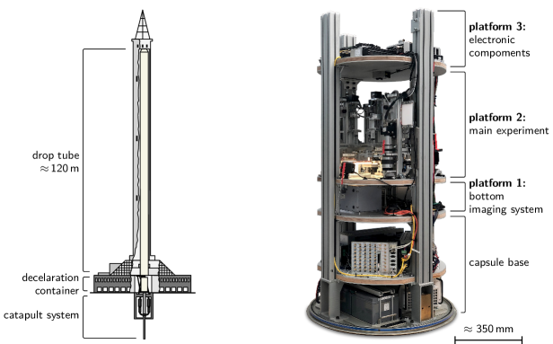
Figure 1: Schematic of the ZARM drop tower (left), and full VIP-DROP² module (right), composed of three experiment platforms and the capsule base. The capsule base houses the control system for drop-tower operations and the battery. Platform 1 contains the high-speed camera recording systems and the camera heads for observations of the droplets from below. Platform 2 contains the main experiment: the droplet deposition areas mounted on a rotary stage, syringe systems for pre-wetting and deposition, and backlighting LED panels. Side-view cameras and a laser unit for PIV are mounted vertically on the stringers. Electronic components on platform 3 include control computers and the laser driver.

The simultaneous deposition of four droplets is made possible by dividing the main experiment platform into four equal sections. Each section allows for the independent preparation and examination of one droplet. Each droplet is deposited on a glass substrate (quartz glass plates from proQuarz GmbH) that can be pre-wetted just before the droplet deposition. Each section is equipped with separate custom-made pump systems for both the deposition and the pre-wetting, so that four different combinations of droplet and (optionally different) pre-wetting material can be examined simultaneously during one flight. A single deposition system (to deposit the droplet) and the associated pre-wetting system are shown in Figure 2.

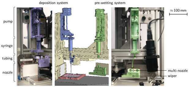
Figure 2: Structure of one section of the main experiment platform: CAD model (center panel), and close-ups of the deposition and pre-wetting system (respectively left and right); the glass substrate in experiment position is also visible.

All pumping systems are controlled individually, which allows to deposit different quantities of liquid at different rate per position. The motor control also implements a configurable amount of retraction of the syringe pistons, in order to stop the deposition of yield-stress fluids as instantaneously as possible: without retraction, the cessation of the flow out of the deposition nozzle produces some leakage that depends on the rheological properties of the fluid. The syringes currently used are $20\text{\,}\mathrm{mL}$ syringes made of polypropylene (PP) from Braun Omnifix; connections are made with polyurethane (PU) tubing of diameter $4\text{\,}\mathrm{mm}$ from SMC Corporation. A purging feature can be implemented (for example, right before launch) to provide clean conditions at the start of the deposition: in the prolonged waiting time prior to experiment start, small quantities of fluid can dry at the tip of the nozzle, or air bubbles can appear in the system. A small recipient is placed on the side on the substrate holder (i.e. attached to the rotary stage; not shown in Fig. 2) in order to retrieve the purged material.

The theoretical resolution of the fluid dispensing is one micro-step of the motor driving the pump, which represents a volume on the order of $10^{-7}$ $\mathrm{L}$. In practice, fluid dispensing precision depends on the viscosity of the fluid, its elasticity, and the total stiffness of the deposition system (notably the tubing and syringe). The dispensing precision is hence estimated from the standard deviation in droplets’ volume (measured for dispensing without retraction); we find a relative standard error of 4% of the deposited volume. The nozzle diameter determines the minimum droplet size of the droplet: droplets of characteristic length $\mathcal{L}\lesssim d_{o}$ would be dominated by surface interaction with the nozzle. For a nozzle outer diameter $d_{o}=$1.2\text{\,}\mathrm{mm}$$, this amounts to a minimum droplet volume of $V_{min}\approx V(\mathcal{L}=2d_{0})=0.058\pm 0.002$ $\mathrm{mL}$.

Each deposition system is equipped with a nozzle that can be precisely adjusted with a linear stage (Thorlabs DT12/M) to be at fixed distance from the substrate. In the current setup, we use commercially available nozzles with inner and outer diameters of respectively $0.8\text{\,}\mathrm{mm}$ and $1.2\text{\,}\mathrm{mm}$ (model “dispensing tip full metal single capillary” from Vieweg). The pre-wetting system is connected to a custom-made combination of a multi-nozzle element and a wiper, which allows the creation of a thin fluid layer covering the substrate (see Sec. III.5).

The general experimental procedure consists of: (1) the deposition of the precursor layer (which should happen in microgravity to ensure homogeneity and reproducible height of the layer), followed by (2) the droplet deposition. The temperature inside the capsule is monitored throughout the experiment by a type K thermocouple, placed on the experiment platform close to one of the deposition nozzles (see Fig. 3). The current setup is intended for fluids whose rheology is only weakly dependent on temperature around ambient conditions, so that no active temperature control is needed.

III.3 Image capture

Different and independent measurements can be conducted simultaneously on each of the four positions. Four cut-outs are made in the main experiment platform, allowing to observe the droplets from below. Therefore, two imaging perspectives are available per position, providing images from the side and from below the droplet, as visible in Figure 3. Corresponding custom-made LED panels ($4000\text{\,}\mathrm{K}$ neutral white LEDs) are placed behind and above the droplets for backlighting, necessary for shadowgraphy and rheo-optical measurements. The LED panel placed above the droplet is pierced to let the nozzle through. For PIV, backlight is not necessary. For recording stress-induced birefringence patterns, the light emitted by the LED panels is polarized by a circular polarizer (Edmund Optics CP42HE) placed in front of the LED panel. Circular polarizers are also placed on the cameras used for rheo-optical measurement.

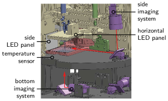
Figure 3: Schematic of the image recording in one experiment section: camera heads for side- and bottom-view images are placed vertically above, and below the glass substrate. Camera view is indicated by red arrows. LED panels to the side and above the deposition areas provide backlight.

High speed cameras are used on all sections. In the current implementation, two Photron FastCam MC-2 recording systems available at ZARM are used, providing four camera heads in total, each with a $512\text{\times}512\text{\,}\mathrm{px}$ CMOS chip recording at $500\text{\,}\mathrm{f}\mathrm{p}\mathrm{s}$. Shadowgraphy uses grayscale images, while rheo-optical measurements use 32-bit color mode. Two additional high speed cameras (Ximea MQ013MG-ON) are used, which have a resolution of $1264\text{\times}1016\text{\,}\mathrm{px}$ at up to $150\text{\,}\mathrm{f}\mathrm{p}\mathrm{s}$ in color mode, and $640\text{\times}512\text{\,}\mathrm{px}$ at up to $500\text{\,}\mathrm{f}\mathrm{p}\mathrm{s}$ in grayscale. Standard lenses are used to obtain a resolution of around $12\text{\,}\mathrm{px}\text{\,}{\mathrm{mm}}^{-1}$ respectively (for the Ximea cameras) $20\text{\,}\mathrm{px}\text{\,}{\mathrm{mm}}^{-1}$.

III.4 Particle image velocimetry

The laser used for PIV is mounted vertically on the main stringer structure, oriented downwards, as shown in Figure 4a. The laser used is a $532\text{\,}\mathrm{nm}$ continuous-wave (CW) diode-pumped solid-state (DPSS) laser (LaserGlow LRS-0532) with optical output power of $500\text{\,}\mathrm{mW}$. A laser sheet is formed from the laser beam using a cylindrical lens (Edmund $12.7\text{\times}12.7\text{\,}\mathrm{mm}$, $-25\text{\,}\mathrm{mm}$ FL, Uncoated Laser Grade PCV), and oriented across the droplet using a $45\mathrm{°}$ mirror (Thorlabs Broadband Dielectric Mirror, $400\text{\,}\mathrm{nm}750\text{\,}\mathrm{nm}$). An optical filter (Thorlabs $625\text{\,}\mathrm{nm}$ CWL, Hard Coated OD 4.0, $50\text{\,}\mathrm{nm}$ Bandpass Filter) is placed on the side-view camera objective to filter out the wavelengths captured besides those emitted by the fluorescent tracer particles, resulting in images similar to the one shown in Figure 4b.

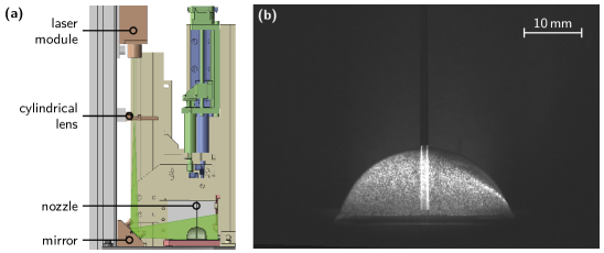
Figure 4: Laser setup and beam guidance. (a) Illustration of the setup, showing the vertically mounted laser unit, the light-sheet optics to the side of the deposition system, together with a deposited droplet on the substrate. (b) Exemplary camera recording from the side of the droplet. In this image, the laser is coming from the left side of the droplet, as pictured in (a).

For additional information on the experimental procedure, three diagnostic cameras (GoPro Hero10) are installed on the main experiment platform. Two are placed to visualize two opposite positions on the setup, while one records the entire experimental platform from above.

III.5 Pre-wetting mechanism

The droplet deposition can be done directly on the substrate or preceded by the deposition of a precursor layer, constituted of either the same or a different fluid. If the film is composed of the same fluid, the analysis can abstract from complicated surface-specific interactions. Under these conditions, a droplet of a Newtonian fluid would evolve from the initial shape toward a completely flat state [52, 28]. Droplets of yield-stress fluids, on the other hand, evolve with time towards a final shape of finite extent, where a balance between surface tension, the material’s yield stress and hydrostatic pressure (in the presence of gravity) is attained [15].

While the precursor layer simplifies the physics of the problem and the associated theory by abstracting from surface-chemistry effects, it poses an experimental challenge: a thin film of the yield-stress fluid needs to be created reproducibly directly before each experiment. In the case of experiments in weightlessness, this typically needs to be attained by an automated procedure just at the beginning of the microgravity phase, to avoid any evaporation effects that would take place over the prolonged preparation time of a microgravity experiment (up to hours), and also since the films cannot be expected to be stable with respect to the strong acceleration at launch.

An automated system allows to deposit a precursor layer on the substrates, prior to the droplet deposition, by depositing a small quantity of material (in form of an array of droplets) and spreading it into a homogeneous film. As mentioned previously, the syringe used for pre-wetting procedure is distinct from that used for the droplet deposition, allowing the precursor layer to be of a different fluid from that of the main droplet.

The pre-wetting mechanism, shown in Figure 5, consists of the assembly of a custom-made array of nozzles (labelled multi-nozzle and manufactured by 3D printing), a fixed steel blade chamfered at $45\mathrm{°}$ to create a defined edge (labelled wiper), and a glass substrate moving under the wiper as the rotary stage rotates. The multi-nozzle first deposits an array of droplets over its full length, which are then mechanically spread as the glass substrate moves under the wiper.

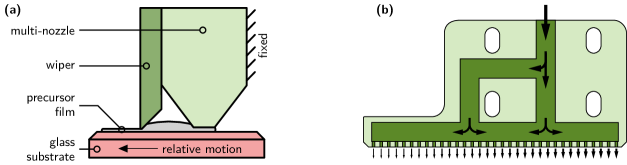
Figure 5: (a) Schematic side-view of the pre-wetting mechanism, consisting of the deposition of a precursor layer. The multi-nozzle is used to deposit fluid on the glass substrate, which is spread into a thin film by the wiper once the glass substrate is moved below it. (b) Multi-nozzle section cut. Arrows indicate the flow direction through the internal channels. The diameters of the outlets decrease towards the center of rotation to equalize the amount of material deposited.

All four glass substrates are fixed to a rotary stage (Zaber X-RSB120AD), which rotates around the center of the main experiment platform. With this, it is possible to execute the pre-wetting procedure on all four positions simultaneously, as the stage rotates by $\approx$80\text{\,}\mathrm{\SIUnitSymbolDegree}$$ clockwise, as depicted in Figure 6.

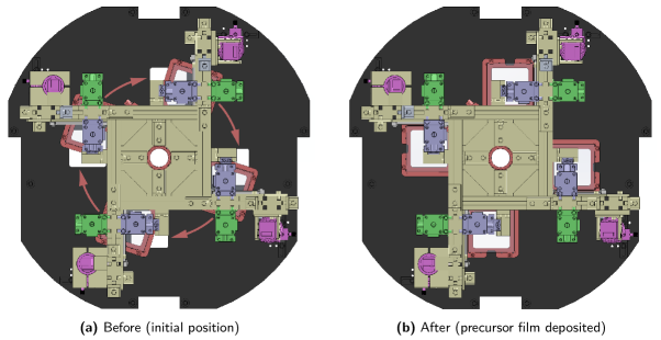
Figure 6: Rotary stage motion during the experiment: (a) Initial position, where the glass substrates are placed right before the wipers; a clockwise rotation of the stage (indicated by arrows) moves the glass substrates underneath the stationary wipers. (b) Final experiment position, where the substrates are centered under the deposition nozzles.

The full pre-wetting procedure takes approximately $1.4\text{\,}\mathrm{s}$ and is executed after the hypergravity phase of the capsule launch. A sequence of snapshots is shown in Figure 7: initially, the rotary stage is positioned such that the inner tip of the blade is in front of the edge of the substrate, ensuring that fluid is spread over the entire glass surface. Given that the arc length of the path described by the wiper blade on the glass substrate increases with increasing distance to the center of rotation, the area on the substrate that needs to be covered by each segment of the wiper also increases with radial position. To homogenize the amount of material spread on the substrate, the multi-nozzle is designed to deposit a radially varying amount of fluid (less on the inner radius, more on the outer radius of the rotary stage) by having increasingly large outlets towards the outer radius (see Fig. 5b).

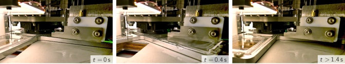
Figure 7: Motion of the rotary stage during the pre-wetting procedure. From left to right: initial pre-wetting position; during rotation; final position under the deposition nozzle. The images are taken from one of the diagnostic cameras installed on the setup.

The homogeneity of the fluid layer depends on multiple factors, including the rheology of the material deposited, the timing and speed of successive events (e.g., onset of deposition of pre-wetting fluid and rotation of the rotary stage), the angle between the wiper and the glass substrate, and the quantity of material deposited by the multi-nozzle. The parameters used for pre-wetting are the following: extrusion flow rate of $4.2\text{\,}\mathrm{mL}\text{\,}{\mathrm{s}}^{-1}$, rotary stage rotation speed of $101\text{\,}\mathrm{\SIUnitSymbolDegree}\text{\,}{\mathrm{s}}^{-1}$, wiper angle of $45\text{\,}\mathrm{\SIUnitSymbolDegree}$ and multi-nozzle internal channel geometry as shown in Fig. 5b.

To test the pre-wetting system, the height variations of an exemplary layer have been probed by optical coherence tomography (OCT) (Thorlabs Telesto Series SD-OCT Systems) for an aqueous solution of Carbopol of 0.55 wt.% (fluid c.6 in Tab. 1). The result is shown in Figure 8 over an area of $8\text{\times}8\text{\,}\mathrm{mm}$ localized in the center of the glass substrate: a resolution of approx. $\pm$ $50\text{\,}\mathrm{\SIUnitSymbolMicro m}$ is achieved for the precursor layer.

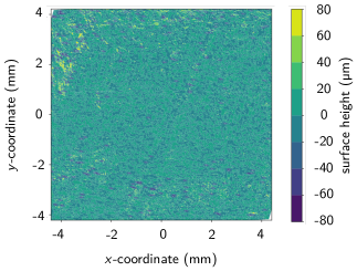
Figure 8: Optical coherence tomography (OCT)analysis of a precursor layer deposited through the automated pre-wetting mechanism. Height variations are measured over an area of $8\text{\times}8\text{\,}\mathrm{mm}$ localized in the center of the glass substrate.

The patterns visible in Fig. 8 most likely originate from partial drying occurring on the fluid layer between deposition and testing (approx. $10\text{\,}\mathrm{min}$); during experiment however, the droplet deposition starts instantaneously after pre-wetting.

III.6 Microgravity considerations

Objects of a certain mass in motion during microgravity prompt the need for an analysis of the residual acceleration and angular velocities of the capsule. Figure 9 presents the acceleration profile (Fig. 9a) and angular velocity (Fig. 9b) for one catapult experiment, where launch happens at $t_{0}=$0\text{\,}\mathrm{s}$$, and the capsule reaches the deceleration pit at $t\approx$9.3\text{\,}\mathrm{s}$$. A standard accelerometer was used to obtain the acceleration (resolution around $10^{-2}g$), hence the precise residual acceleration in microgravity cannot be obtained from this measurement.

Note that the overall volume of fluid that is deposited (on the order of $20\text{\,}\mathrm{mL}$) is small enough that no influence on the $\mu g$ quality is expected. However, the rotary stage motion causes a counter-rotation of the entire capsule due to conservation of angular momentum. This is visible in the angular velocity around the $z$-axis (Fig. 9b): the $z$-axis angular velocity shows a small plateau lasting until $t\approx$2\text{\,}\mathrm{s}$$, which corresponds to the end of the rotary stage motion. After that, the angular velocity remains at a stable small value (around $0.02\text{\,}\mathrm{rad}\text{\,}{\mathrm{s}}^{-1}$) typical for catapult launches [53]).

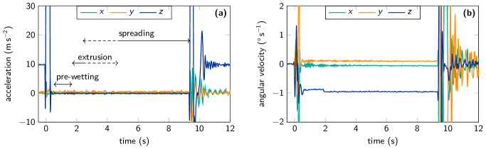
Figure 9: Accelerometer and gyroscope data, recorded by the internal measurement unit placed inside the capsule during catapult launch, where the launch happens at $\mathsf{t_{0}}=$0\text{\,}\mathrm{s}$$. (a) Acceleration of the capsule and (b) angular velocity in Cartesian coordinate directions. The steps of the experiment and their duration are given in (a); the duration of extrusion varies with droplet size and extrusion speed: extreme values are represented by the start and end of dashed line).

IV Results

The vip-drop² module was used on three campaigns at ZARM between November 2021 and June 2022, hence producing data both on-ground and in microgravity, using the drop tower’s catapult system. We report here preliminary data analysis to exemplify the capabilities of the module. A more in-depth discussion of physical effects will be provided elsewhere. Data obtained under microgravity conditions is labeled $\mu g$, and corresponding ground experiment is labeled $1g$.

Two material classes are used during experiments. Shadowgraphy and PIV are performed on aqueous solution of poly acrylic acid (PAA) (referred to in the following under its commercial name Carbopol). The stress-optical measurements are performed on micellar solutions of cetyltrimethylammoniumbromide (CTAB) and sodium salicylate (NaSal) at varying concentrations, keeping the CTAB/NaSal ratio fixed at $5/3$.

IV.1 Experimental fluids: Carbopol solutions

Carbopol aqueous solutions are widely studied as model viscoplastic fluids with well characterized bulk rheology (see among others Refs. [15, 38, 54, 55, 56]). The solutions are prepared from a master batch (PAA from Sigma Aldrich mixed in MilliQ water), diluted into six different concentrations, providing fluids with yield stresses $\tau_{0}\in[$6.5\text{\,}\mathrm{Pa}$,\,$55\text{\,}\mathrm{Pa}$]$. The mixing procedure is detailed in supplementary material (Sec. V.1).

The specific parameters of the six solutions are given in Table 1; the rheological properties of the fluids were obtained using an Anton Paar rheometer (MCR 502). Shear rheology (varying the shear rate within $[$0.01\text{\,}{\mathrm{s}}^{-1}$,\,$1000\text{\,}{\mathrm{s}}^{-1}$]$ were performed and the values of yield stress were obtained by fitting a Herschel-Bulkley fit through the flow curve data (Tab. 1).

The surface tension of yield stress fluids is challenging to determine experimentally [57, 58]. For Carbopol, we use the surface tension of water ($\sigma\approx$0.07\text{\,}\mathrm{N}\text{\,}{\mathrm{m}}^{-1}$$) [57, 15]

Table 1: Experimental parameters for the Carbopol aqueous solutions used in experiments.

Fluid	Composition	Yield stress
Fluid c.1	0.3 wt%	$6.5\text{\,}\mathrm{Pa}$
Fluid c.2	0.35 wt%	$9\text{\,}\mathrm{Pa}$
Fluid c.3	0.4 wt%	$14\text{\,}\mathrm{Pa}$
Fluid c.4	0.45 wt%	$21\text{\,}\mathrm{Pa}$
Fluid c.5	0.5 wt%	$35\text{\,}\mathrm{Pa}$
Fluid c.6	0.55 wt%	$55\text{\,}\mathrm{Pa}$

IV.2 Experimental fluids: micellar solutions

The stress-optical measurements are performed on micellar solutions of CTAB and NaSal at varying concentrations, keeping the CTAB/NaSal ratio fixed at $5/3$. These micellar solutions are exemplary shear-thinning viscoelastic fluids that exhibit a large photoelastic constant $C$. The stress-optical coefficient $C$ depends only on the local structure of the polymer [59] and has indeed been found to be essentially independent on the CTAB/NaSal concentration, $C\approx-3.1\cdot 10^{-7}$ ${\mathrm{Pa}}^{-1}$ [60]. We neglect small nonlinearities that are in principle present at high flow rates [61].

Using CTAB/NaSal solutions of the same mixing ratio, Gladden and Belmonte demonstrated rheo-optical measurements of the stresses around a moving object in a study of cutting and tearing of gel [62] and of shear waves in the fluid [42]; an equimolar mixture of cetylpyridinium chloride (CPCl) and NaSal was used by Handzy and Belmonte [63] to visualize the stresses around rising bubbles in a viscoelastic fluid.

Changing the concentration of both CTAB and NaSal, we adjust the viscoelasticity of the solutions [64]. The fixed mixing ratio ensures that the fluid remains in the homogeneously flowing regime of wormlike micelles [65]. The parameters of the stress-birefringent fluids used in experiments are summarized in Table 2.

Table 2: Parameters of the micellar solutions used as stress birefringent materials in experiments. Values for viscosity, structural relaxation time and apparent yield stress are estimated from literature: ^a Gladden and Belmonte [62]; ^b Gladden, Skelton, and Mobley [42]; ^c Hartmann and Cressely [64].

Fluid	Composition (CTAB/NaSal)	Viscosity	Relaxation time	Apparent yield stress
Fluid sb.1	200/120 $\mathrm{m\textsc{m}}$	$167\text{\,}\mathrm{Pa}\text{\,}\mathrm{s}$ a	$1\text{\,}\mathrm{s}$ b	$150\text{\,}\mathrm{Pa}$ b
Fluid sb.2	160/96 $\mathrm{m\textsc{m}}$	–$\text{\,}$	–	–
Fluid sb.3	120/72 $\mathrm{m\textsc{m}}$	–$\text{\,}$	–	–
Fluid sb.4	100/60 $\mathrm{m\textsc{m}}$	$1200\text{\,}\mathrm{Pa}\text{\,}\mathrm{s}$ c	$30\text{\,}\mathrm{s}$ c	$40\text{\,}\mathrm{Pa}$ c
Fluid sb.5	80/48 $\mathrm{m\textsc{m}}$	–	–	–

IV.3 Experimental parameters

Droplets of various sizes are deposited, characterized by the length scale $\mathcal{L}$, which corresponds to the radius of a perfect sphere of the same volume as the droplet deposited – in other words, for a droplet of volume $V$, $\mathcal{L}={(3V/4\pi)}^{1/3}$. The rheology of the experimental fluids is characterized by the plastocapillary number

$$\mathcal{J}=\frac{\tau_{0}\,\mathcal{L}}{\sigma},$$ (3)

which compares the yield stress $\tau_{0}$ of the fluid to its capillary pressure. The extrusion speed at which droplets are deposited can also be varied; the parameters that we have tested are summarized in Table 3. It is noteworthy that a short phase of retraction after the deposition can be implemented to ensure full arrest of the extrusion.

Table 3: Extrusion flow rates used in the vip-drop² module during experimental campaigns.

Extrusion flow rates
$Q_{0}=5.97\cdot 10^{-1}$ $\mathrm{mL}\text{\,}{\mathrm{s}}^{-1}$
$Q_{1}=2.39$ $\mathrm{mL}\text{\,}{\mathrm{s}}^{-1}$
$Q_{2}=4.77$ $\mathrm{mL}\text{\,}{\mathrm{s}}^{-1}$

Finally, the Bond number defined in Eq. 1 is used to characterize the regime in which each experiment is conducted. For experiments conducted under microgravity, $B$ is calculated using $g_{\mu g}=$9.81\text{\cdot}{10}^{-4}\text{\,}\mathrm{m}\text{\,}{\mathrm{s}}^{-1}\text{\,}{\mathrm{}}^{2}$$, which corresponds to the average gravitational acceleration during catapult experiments. The volume $V$ of each droplet (hence its true characteristic length) is calculated from the final shape of the droplet by image analysis, assuming axisymmetry.

IV.4 Shadowgraphy

Exemplary shadowgraphy images of Carpobol solution droplets are shown in Figure 10. The images are taken at various times after the start of the fluid deposition; note that extrusion is not complete at the time when the first image is taken. The images labeled $1g$ and $\mu g$ are respectively from on-ground and microgravity repetitions of the experiment under the same parameters. Visual inspection of the images already demonstrates the effect of hydrostatic pressure in the $1g$ experiment, flattening the droplet while under microgravity conditions it retains its initial dome-like shape.

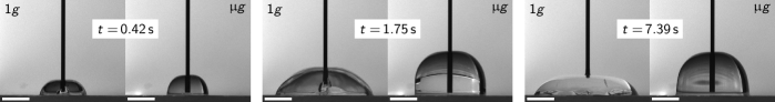
Figure 10: Exemplary shadowgraphy images for the carbopol dispersion c.5 (see Table 1), on ground ($1g$) and under microgravity conditions ($\mu g$). The droplet has a final volume $V=$ $2.7\text{\,}\mathrm{mL}$. The scale bar on each picture represents $8\text{\,}\mathrm{mm}$.

The simplest quantity to extract from the shadowgraphy experiment is the radius of a droplet as a function of time, $R(t)$, easily accessible by image analysis. Figure 11 shows exemplary evolutions of $R(t)$, where $t=$0\text{\,}\mathrm{s}$$ is the time at which extrusion effectively starts. The droplets’ volume is estimated using the Sessile Drop Analysis Python algorithm by van Gorcum [67, 66]. Eight experiments are represented: in Fig. 11a, droplets of fluid c.2 ($\tau_{0}=$9\text{\,}\mathrm{Pa}$$) are analyzed; in Fig. 11b, data corresponding to fluid c.5 ($\tau_{0}=$35\text{\,}\mathrm{Pa}$$) is shown. The four curves in each graph correspond to two droplet sizes (characteristic lengths $\mathcal{L}$ of approx. $4.5\text{\,}\mathrm{mm}$ and $10\text{\,}\mathrm{mm}$; orange respectively green symbols in Fig. 11a, and red respectively blue symbols in Fig. 11b), under Earth gravity and microgravity (full and empty marks, respectively). Besides the graphs, Fig. 11 shows images of the analyzed droplets, at a time well inside the stationary regime of $R(t)$.

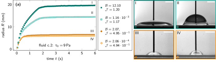
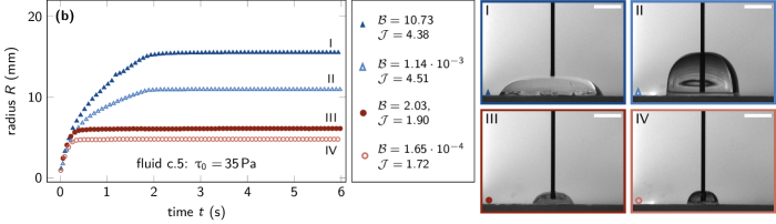
Figure 11: Radius $R(t)$ of the droplets as a function of time $t$, comparing the same fluids on-ground (labelled $1g$, filled marks) and under microgravity conditions ($\mu g$, empty marks). (a) For fluid c.2, aqueous solution of 0.5 wt% Carbopol, and (b) for fluid c.5, aqueous solution of 0.35 wt% Carbopol, for two droplets of characteristic lengths $\mathcal{L}\approx 9.43\pm 0.28$ $\mathrm{mm}$ and $\mathcal{L}\approx 3.92\pm 0.25$ $\mathrm{mm}$, respectively for (a) green squares and orange diamonds, and for (b) blue triangles and red circles. Pictures are taken at the last instant before the end of the experiment. In all pictures, the scale bar represents $8\text{\,}\mathrm{mm}$.

The data demonstrate the influence of gravity on the droplet spreading clearly, where in both cases, the fluid spreads faster in the presence of gravitationally-induced hydrostatic pressure.

Because for a yield stress fluid, the spreading stops at a finite droplet radius, there results a finite apparent macroscopic contact angle between the surface-wetting layer and the droplet, even if both are of the same fluid (and furnish zero microscopic contact angle). The apparent contact angle $\theta$ between the droplet and the precursor layer depends on the material properties, and it is also modified by the gravitational environment. We have extracted $\theta$ by image analysis [67, 66] from the shadowgraphy images presented in Fig. 11a and 11b as I to IV: from local linear fits to the droplet profile, the value corresponding to the maximum slope is taken as the apparent contact angle. These values are reported in Figure 12.

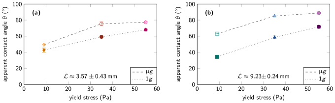
Figure 12: Apparent contact angle $\theta$ between the droplets and the precursor layer, for droplets of characteristic length (a) $\mathcal{L}\approx 3.51\pm 0.43$ $\mathrm{mm}$ and (b) $\mathcal{L}\approx 11.16\pm 2.13$ $\mathrm{mm}$. Lines are a help to the eye, distinguishing $\mu g$ (dashed line, open symbols) and $1g$ (dotted line, filled symbols) data sets. Error bars are the standard deviation on measured $\theta$.

The increase of apparent contact angle $\theta$ with droplets’ radius and yield stress is in accordance with previous work [56]; our results allow to consider additionally the gravitational acceleration as a variable parameter. Again, the effect of gravity is evident: hydrostatic pressure causes a decrease in the contact angle, which is more pronounced for droplets of large characteristic length (Fig. 12b).

IV.5 Particle image velocimetry (PIV)

For PIV, some of the carbopol solutions were seeded with fluorescent-labeled tracer particles. The tracers are $10\text{\,}\mathrm{\SIUnitSymbolMicro m}$ diameter polystyrene (PS) particles from MicroParticles GmbH (product PS-FluoRed-10.0). Polymerized with organic fluorescent dyes, they absorb light at a wavelength around the laser excitation of $532\text{\,}\mathrm{nm}$, and emit fluorescence light at a wave length of $607\text{\,}\mathrm{nm}$.

Exemplary velocity-field reconstructions for a point $t=$2\text{\,}\mathrm{s}$$ at the end of the extrusion phase are shown in Figure 13. The droplet side view was recorded at $50\text{\,}\mathrm{fps}$, and PIV was performed using two consecutive frames using the software OpenPIV (version 0.23.8) [68]. Images were masked with a threshold map to darken the area outside the droplet. The snapshots in Figure 13 feature the moment at the end of the extrusion phase when the droplets spreading is strongly slowed down, and the pump is about to stop; hence, a localized flow near the nozzle appears.

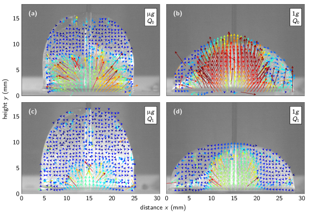
Figure 13: Exemplary PIV reconstructions of the velocity fields inside carbopol droplets (material c.6, characteristic length $\mathcal{L}\approx$10\text{\,}\mathrm{mm}$$), $t=$2\text{\,}\mathrm{s}$$ after start of the droplet deposition. The top panels (a) and (b) correspond to an extrusion speed $Q_{1}=$2.39\text{\,}\mathrm{mL}\text{\,}{\mathrm{s}}^{-1}$$ in $\mu g$ and $1g$ conditions, respectively; bottom panels (c) and (d) to $Q_{2}=$4.77\text{\,}\mathrm{mL}\text{\,}{\mathrm{s}}^{-1}$$. The arrows indicating the in-plane velocity field are colored according to increasing magnitude (blue to red in the range $v=$0\text{\,}\mathrm{mm}\text{\,}{\mathrm{s}}^{-1}$$ to $v=$3\text{\,}\mathrm{mm}\text{\,}{\mathrm{s}}^{-1}$$). Droplet images are to scale within the plots’ axes.

The velocity fields under $1g$ show the appearance of a region with a significantly smaller velocity on the outer surface of the droplets, separated from the inner moving part of the fluid by a sharply defined yield surface. For the flatter droplet extruded at a higher speed (Fig. 13 bottom), the location of this yield surface is closer to the center of the droplet.

A striking difference is seen in comparison to the droplets deposited in microgravity (Fig. 13 left): here, the zero-velocity regime covers the entire top of the droplet. The absence of hydrostatic pressure allows the unyielded fluid to remain on top of the droplet, without being pushed to the sides as it is the case in $1g$.

Note that for flat droplets with a large bottom area, performing PIV from the side has the drawback that due to a “lens effect” caused by total inner reflection, dark regions appear in some of the PIV images. This is partially mitigated by placing the laser sheet slightly less centered for large droplets (to avoid crossing the nozzle). It limits the application of PIV to fluids of sufficiently high yield stress, where the resulting droplet shapes are more less flat.

Also visible in Fig. 13 is a “shadow” effect to the left of the deposition needle in the top part of the droplets. This shadow is caused by the needle, and limits the information that can be obtained from the left half of the droplet. However, as seen in Fig. 13(b), even in the shadow region a reconstruction of the velocity field is still possible within reasonable limitations.

IV.6 Rheo-optical measurement

A detailed analysis of the rheo-optical data obtained from our setup is beyond the scope of the present contribution. We only show here a set of exemplary images to allow for a qualitative assessment.

In Figure 14, droplets of the micellar fluid sb. 1 (CTAB/NaSal 200/120 $\mathrm{m\textsc{m}}$) are shown at three representative instants in the experiment: first, shortly after the effective start of extrusion; then right before the end of extrusion; finally, in the last instant preceding impact for the microgravity case, and at the exact same time for the ground one. The fluid is deposited at an extrusion flow rate of $7.5\cdot 10^{-3}$ $\mathrm{m}\text{\,}{\mathrm{s}}^{-1}$. In all pictures presented, the droplets are deposited directly on the glass substrate, without precursor layer.

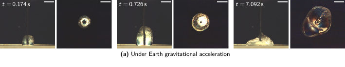
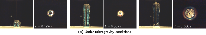
Figure 14: Droplets of micellar fluid exhibiting stress birefringence patterns, (a) on-ground and (b) under microgravity conditions, for the fluid sb. 1 (CTAB/NaSal 200/120 $\mathrm{m\textsc{m}}$). On both levels of gravitational acceleration, material extrusion was done at $7.5\text{\cdot}{10}^{-3}\text{\,}\mathrm{m}\text{\,}{\mathrm{s}}^{-1}$. Time $t$ is given as time since $t_{0}=$0\text{\,}\mathrm{s}$$ the effective start of extrusion. The scale bar on each image represents $8\text{\,}\mathrm{mm}$.

From the exemplary images presented, one can see that there is a dramatic effect of the deposition rate for the micellar fluid, both on the shape of the droplet and on the magnitude of the internal stresses. In particular, for the faster deposition rate, we observe the formation of a high “pillar” of the viscoelastic fluid under microgravity conditions, that remains stable over the time scale of the experiment. The same material, with the same extrusion speed, but on-ground, forms much flatter droplets, demonstrating the role of microgravity conditions to stabilize the extrusion of tall structures of a soft material.

A rough estimate of the stresses from the blue-ish color clearly visible in fig. 14, making use of suitable interference color charts [69], confirms that the internal stresses are comparable to the yield stress of the material, around $10\text{\,}\mathrm{Pa}50\text{\,}\mathrm{Pa}$.

V Conclusion

We have described our implementation of the vip-drop² drop-tower module to study the spreading of complex fluids under microgravity. The motivation to perform such studies is given by the fact that droplet spreading in the presence of gravity, i.e., at finite Bond number, is notably different from the spreading in the surface-tension dominated regime at $\mathcal{B}\rightarrow 0$. The latter regime is of interest for many technological applications, among which AM. Performing experiments under microgravity conditions, large droplets can be used to carry out optical analyses of droplet shapes, internal velocity and stress fields, while maintaining small Bond numbers. The microgravity experiment essentially achieves to decouple the limit an ultimately of $\mathcal{B}\rightarrow 0$ from the material and deposition parameters of the yield-stress fluids.

A more detailed analysis of the results provided by our drop-tower module will address the comparison with scaling laws predicted by the thin-film solutions of the Navier-Stokes equations for viscoplastic fluids. It is expected, that the case $\mathcal{B}=0$ is governed by different scaling exponents, and achieving this limit with large droplets will allow to verify the scaling law without being hampered by experimental artifacts arising from small droplets.

The PIV measurements can be used to determine the gravity-dependence of the yield surface inside the droplet, separating the region of plastic flow in the region with large stresses from the “plug” flow in the region where the stresses remain below the yield stress. Future extensions of the setup could include particle tracking velocimetry (PTV), a Lagrangian method where the tracer particles are individually tracked. Suitable methods have been developed for droplets, including astigmatic PTV [70], which allows the tracking in 3D with a single camera, utilizing its astigmatic imaging defects to reconstruct out-of-focal plane positions. OCT has also allowed to study the flow fields of evaporating droplets at various inclination angles (and hence various effective gravity levels) [71], and could be added in a future implementation of the experiment.

We aim to establish the analysis of stress-induced birefringence in droplets of yield-stress fluids (or shear-thinning viscoelastic fluids with a large apparent yield stress) as a qualitative, and ultimately a quantitative tool to predict internal stresses in yield-stress materials. To this end, the birefringent images obtained in our experiment will be compared to computer simulation combined with ray tracing, potentially using machine learning to address the inverse problem of reconstructing the internal stress field from the experimental images.

For the present analysis, we have largely ignored the dynamics of the droplet in the moment of impact at the end of the drop-tower flight. These moments under strong hypergravity conditions could potentially be exploited further to provide data on the effect of external acceleration on the fluid’s spread, such as in centrifugal casting or density-based separation methods.

Further developments could include an adaptation of the experimental module for different microgravity platforms in order to provide longer time in weightlessness, for example to study the deposition of filaments of viscoplastic materials that are relevant for AM and bioprinting. Possible platforms include sounding rockets, which providing several minutes of experiment time in weightlessness.

Supplementary material

V.1 Mixing protocol for Carbopol solutions

For Carbopol suspensions, premixed aqueous solution of 1 wt% of poly acrylic acid (PAA)polymer (Sigma Aldrich) was first prepared: poly acrylic acid (PAA)powders were mixed with Milli-Q water using a four-blade marine impeller (1000-1500 rpm) at room temperature. The mixture was pH-neutralized with triethanolamin (Sigma Aldrich). The premixed batch was then diluted to the final concentrations listed in table 1. Bubbles were removed from the sample by centrifuging the fluids at $2200\text{\,}\mathrm{rpm}$ for $20\text{\,}\mathrm{min}$.

V.2 Mixing protocol for micellar solutions

The aqueous wormlike micellar solutions are obtained from cetyltrimethylammoniumbromide (CTAB)in powder ($\geq 99\%$ pure $\mathrm{C_{19}H_{42}BrN}$, Carl Roth) and sodium salicylate (NaSal)($99\%$ pure $\mathrm{C_{7}H_{5}NaO_{3}}$, ThermoFisher Scientific). Each powder is individually dissolved in distilled water at $70\text{\,}\mathrm{\SIUnitSymbolCelsius}$ and strongly stirred until full dissolution of the powder is the water (with a minimum of $30\text{\,}\mathrm{min}$). Then both fluids are mixed; the mixture is covered and strongly stirred for for $1\text{\,}\mathrm{h}$ at $70\text{\,}\mathrm{\SIUnitSymbolCelsius}$, before being let to cool down for at least one day before use. Bubbles are suppressed by centrifuging the fluids at $7000\text{\,}\mathrm{rpm}$ for $10\text{\,}\mathrm{min}$.

V.3 Videos

Videos are provided as supplementary material to illustrate the droplet deposition under Earth gravity and microgravity conditions. For all videos, the calibration bar corresponds to a length of $8\text{\,}\mathrm{mm}$ and the video is slowed down by a factor of two. The videos provided correspond to the following experiments:

• Fluid c.1 (lowest yield stress), droplet of characteristic length $\mathcal{L}=9.92\pm 0.04$ $\mathrm{mm}$, extrusion flow rate $Q_{1}=$2.39\text{\,}\mathrm{mL}\text{\,}{\mathrm{s}}^{-1}$$; on-ground (left) and in microgravity (right).

• Fluid c.6 (highest yield stress), droplet of characteristic length $\mathcal{L}=10.30\pm 0.11$ $\mathrm{mm}$, extrusion flow rate $Q_{1}=$2.39\text{\,}\mathrm{mL}\text{\,}{\mathrm{s}}^{-1}$$; on-ground (left) and in microgravity (right).

• Fluid sb. 1 (CTAB/NaSal 200/120 $\mathrm{m\textsc{m}}$), droplet of characteristic length $\mathcal{L}=6.95\pm 0.01$ $\mathrm{mm}$, extrusion flow rate $Q_{1}=$2.39\text{\,}\mathrm{mL}\text{\,}{\mathrm{s}}^{-1}$$; on-ground (top, both panels) and in microgravity (bottom, both panels). For both gravitational accelerations, the two panels placed side by side are the side (left) and bottom (right) views of the same droplet.

Author declarations

The authors have no conflicts to disclose.

Data availability

All data is available from the corresponding author upon reasonable request.

References

References

- Placone and Engler [2018] J. K. Placone and A. J. Engler, “Recent advances in extrusion-based 3D printing for biomedical applications,” Advanced healthcare materials 7, 1701161 (2018).
- Kyle et al. [2017] S. Kyle, Z. M. Jessop, A. Al-Sabah, and I. S. Whitaker, “Printability of candidate biomaterials for extrusion based 3D printing: state of the art,” Advanced healthcare materials 6, 1700264 (2017).
- Jiang et al. [2020] Z. Jiang, B. Diggle, M. L. Tan, J. Viktorova, C. W. Bennett, and L. A. Connal, “Extrusion 3D printing of polymeric materials with advanced properties,” Advanced Science 7, 2001379 (2020).
- Buswell et al. [2018] R. A. Buswell, W. L. De Silva, S. Z. Jones, and J. Dirrenberger, “3D printing using concrete extrusion: A roadmap for research,” Cement and Concrete Research 112, 37–49 (2018).
- Weinstein and Ruschak [2004] S. J. Weinstein and K. J. Ruschak, “Coating flows,” Annu. Rev. Fluid Mech. 36, 29–53 (2004).
- Ruschak [1985] K. J. Ruschak, “Coating flows,” Annual Review of Fluid Mechanics 17, 65–89 (1985).
- Derby [2010] B. Derby, “Inkjet printing of functional and structural materials: fluid property requirements, feature stability, and resolution,” Annual Review of Materials Research 40, 395–414 (2010).
- Lohse [2022] D. Lohse, “Fundamental fluid dynamics challenges in inkjet printing,” Annual Review of Fluid Mechanics 54, 349–382 (2022).
- Yonemoto and Kunugi [2017] Y. Yonemoto and T. Kunugi, “Analytical consideration of liquid droplet impingement on solid surfaces,” Scientific Reports 7, 2362 (2017).
- Ueda, Enomoto, and Kanetsuki [1979] T. Ueda, T. Enomoto, and M. Kanetsuki, “Heat transfer characteristics and dynamic behavior of saturated droplets impinging on a heated vertical surface,” Bulletin of JSME 22, 724–732 (1979).
- Lu, Wang, and Duan [2016] G. Lu, X.-D. Wang, and Y.-Y. Duan, “A critical review of dynamic wetting by complex fluids: from newtonian fluids to non-newtonian fluids and nanofluids,” Advances in colloid and interface science 236, 43–62 (2016).
- Rafaı and Bonn [2005] S. Rafaı and D. Bonn, “Spreading of non-newtonian fluids and surfactant solutions on solid surfaces,” Physica A: Statistical Mechanics and its Applications 358, 58–67 (2005).
- Bonn et al. [2009] D. Bonn, J. Eggers, J. Indekeu, J. Meunier, and E. Rolley, “Wetting and spreading,” Reviews of modern physics 81, 739 (2009).
- Bergeron et al. [2000] V. Bergeron, D. Bonn, J. Y. Martin, and L. Vovelle, “Controlling droplet deposition with polymer additives,” Nature 405, 772–775 (2000).
- Jalaal, Stoeber, and Balmforth [2020] M. Jalaal, B. Stoeber, and N. J. Balmforth, “Spreading of viscoplastic droplets,” J. Fluid Mech. 914, A21 (2020).
- Griffiths [2000] R. W. Griffiths, “The dynamics of lava flows,” Annu. Rev. Fluid Mech. 32, 477–518 (2000).
- Bassis and Ultee [2019] J. N. Bassis and L. Ultee, “A thin film viscoplastic theory for calving glaciers: Toward a bound on the calving rate of glaciers,” J. Geophys. Res.: Earth Surface 124, 2036–2055 (2019).
- Wong and Pfahnl [2014] J. Y. Wong and A. C. Pfahnl, “3D printing of surgical instruments for long-duration space missions,” Aviation, space, and environmental medicine 85, 758–763 (2014).
- Joshi and Sheikh [2015] S. C. Joshi and A. A. Sheikh, “3D printing in aerospace and its long-term sustainability,” Virtual and Physical Prototyping 10, 175–185 (2015).
- Dunn et al. [2010] J. J. Dunn, D. N. Hutchison, A. M. Kemmer, A. Z. Ellsworth, M. Snyder, W. B. White, and B. R. Blair, “3D printing in space: enabling new markets and accelerating the growth of orbital infrastructure,” Proc. Space Manufacturing 14, 29–31 (2010).
- Leach [2014] N. Leach, “3D printing in space,” Architectural Design 84, 108–113 (2014).
- Makaya et al. [2022] A. Makaya, L. Pambaguian, T. Ghidini, T. Rohr, U. Lafont, and A. Meurisse, “Towards out of earth manufacturing: overview of the ESA materials and processes activities on manufacturing in space,” CEAS Space Journal (2022), 10.1007/s12567-022-00428-1.
- Dittus [1991] H. Dittus, “Drop tower ‘Bremen’: a weightlessness laboratory on Earth,” Endeavour, New Series 15, 72–78 (1991).
- von Kampen, Kaczmarczik, and Rath [2006] P. von Kampen, U. Kaczmarczik, and H. J. Rath, “The new drop tower catapult system,” Acta Astronautica 59, 278–283 (2006).
- Pletser [2016] V. Pletser, “European aircraft parabolic flights for microgravity research, applications and exploration: A review,” REACH 1, 11–19 (2016).
- Segal et al. [2018] C. Segal, M. Pallone, M. Pontani, P. Teofilatto, and A. Minotti, “Design methodology and performance evaluation of new generation sounding rockets,” International Journal of Aerospace Engineering 2018, 1678709 (2018).
- Dittus and Schomisch [1990] H. Dittus and A. Schomisch, “Vacuum systems for microgravity experiments,” Vacuum 41, 2135–2137 (1990).
- Bergemann, Juel, and Heil [2018] N. Bergemann, A. Juel, and M. Heil, “Viscous drops on a layer of the same fluid: from sinking, wedging and spreading to their long-time evolution,” Journal of Fluid Mechanics 843, 1–28 (2018).
- Diana et al. [2012] A. Diana, M. Castillo, D. Brutin, and T. Steinberg, “Sessile drop wettability in normal and reduced gravity,” Microgravity Science and Technology 24, 195–202 (2012).
- Brutin et al. [2009] D. Brutin, Z. Zhu, O. Rahli, J. Xie, Q. Liu, and L. Tadrist, “Sessile drop in microgravity: Creation, contact angle and interface,” Microgravity Science and Technology 21, 67–76 (2009).
- Abel, Ross, and Andrzejewski [2004] G. Abel, G. G. Ross, and L. Andrzejewski, “Wetting of a liquid surface by another immiscible liquid in microgravity,” Advances in Space Research 33, 1431–1438 (2004).
- Ababneh, Amirfazli, and Elliott [2006] A. Ababneh, A. Amirfazli, and J. A. W. Elliott, “Effect of gravity on the macroscopic advancing contact angle of sessile drops,” The Canadian Journal of Chemical Engineering 84, 39–43 (2006).
- Kabov and Zaitsev [2013] O. A. Kabov and D. V. Zaitsev, “The effect of wetting hysteresis on drop spreading under gravity,” Doklady Physics 58, 292–295 (2013).
- Carle, Sobac, and Brutin [2013] F. Carle, B. Sobac, and D. Brutin, “Experimental evidence of the atmospheric convective transport contribution to sessile droplet evaporation,” Applied Physics Letters 102, 061603 (2013).
- Kumar et al. [2020] S. Kumar, M. Medale, P. D. Marco, and D. Brutin, “Sessile volatile drop evaporation under microgravity,” npj Microgravity 6, 37 (2020).
- Li, Lan, and Wang [2020] W. Li, D. Lan, and Y. Wang, “Exploration of direct-ink-write 3d printing in space: Droplet dynamics and patterns formation in microgravity,” Microgravity Science and Technology 32, 935–940 (2020).
- Huang et al. [2021] J. Huang, L. Qi, J. Luo, and X. Hou, “Insights into the impact and solidification of metal droplets in ground-based investigation of droplet deposition 3d printing under microgravity,” Applied Thermal Engineering 183, 116176 (2021).
- Bonn et al. [2017] D. Bonn, M. M. Denn, L. Berthier, T. Divoux, and S. Manneville, “Yield stress materials in soft condensed matter,” Reviews of Modern Physics 89, 035005 (2017).
- Balmforth, Frigaard, and Ovarlez [2014] N. J. Balmforth, I. A. Frigaard, and G. Ovarlez, “Yielding to stress: recent developments in viscoplastic fluid mechanics,” Annual Review of Fluid Mechanics 46, 121–146 (2014).
- Amador et al. [2016] C. Amador, B. L. Otilio, R. R. Kinnick, and M. W. Urban, “Ultrasonic method to characterize shear wave propagation in micellar fluids,” The Journal of the Acoustical Society of America 140, 1719–1726 (2016).
- Chen et al. [2022] Q. Chen, F. Restagno, D. Langevin, and A. Salonen, “The rise of bubbles in shear thinning viscoelastic fluids,” Journal of Colloid and Interface Science 616, 360–368 (2022).
- Gladden, Skelton, and Mobley [2010] J. R. Gladden, C. E. Skelton, and J. Mobley, “Shear waves in viscoelastic wormlike micellar fluids,” J. Acoust. Soc. Am. 128, EL268–EL273 (2010).
- Adrian [1991] R. J. Adrian, “Particle-imaging techniques for experimental fluid mechanics,” Annu. Rev. Fluid Mech. 23, 261–304 (1991).
- Westerweel, Elsinga, and Adrian [2013] J. Westerweel, G. E. Elsinga, and R. J. Adrian, “Particle image velocimetry for complex and turbulent flows,” Annu. Rev. Fluid Mech. 45, 409–436 (2013).
- Raffel et al. [2007] M. Raffel, C. E. Willert, F. Scarano, C. J. Kähler, S. T. Wereley, and J. Kompenhans, Particle Image Velocimetry, third edition ed. (Springer, Berlin, 2007).
- Jalaal, Balmforth, and Stoeber [2015] M. Jalaal, N. J. Balmforth, and B. Stoeber, “Slip of spreading viscoplastic droplets,” Langmuir 31, 12071–12075 (2015).
- Leven [1969] M. M. Leven, ed., Photoelasticity: The Selected Scientific Papers of M. M. Frocht (Pergamon Press, Oxford, 1969).
- Ramesh [2000] K. Ramesh, Digital Photoelasticity (Springer-Verlag, Berlin, 2000).
- Soulages et al. [2008] J. Soulages, T. Schweizer, D. C. Venerus, J. Hostettler, F. Mettler, M. Kröger, and H. C. Öttinger, “Lubricated optical rheometer for the study of two-dimensional complex flows of polymer melts,” J. Non-Newt. Fluid Mech. 150, 43–55 (2008).
- Abed Zadeh et al. [2019] A. Abed Zadeh, J. Barés, T. A. Brzinski, K. E. Daniels, J. Dijksman, N. Docquier, H. O. Everitt, J. E. Kollmer, O. Lantsoght, D. Wang, M. Workamp, Y. Zhao, and H. Zheng, “Enlightening force chains: a review of photoelasticimetry in granular matter,” Granular Matter 21, 83 (2019).
- Garg et al. [2021] A. Garg, N. Bergemann, B. Smith, M. Heil, and A. Juel, “Fluidisation of yield stress fluids under vibration,” J. Non-Newt. Fluid Mech. 294, 104595 (2021).
- Jalaal, Seyfert, and Snoeijer [2019] M. Jalaal, C. Seyfert, and J. Snoeijer, “Capillary ripples in thin viscous films,” J. Fluid Mech. 880, 430–440 (2019).
- Selig, Dittus, and Lämmerzahl [2010] H. Selig, H. Dittus, and C. Lämmerzahl, “Drop tower microgravity improvement towards the nano-g level for the MICROSCOPE payload tests,” Micrograv. Sci. Technol. 22, 539–549 (2010).
- Frigaard [2019] I. Frigaard, “Simple yield stress fluids,” Current Opinion in Colloid & Interface Science 43, 80–93 (2019).
- Jalaal, Kemper, and Lohse [2019] M. Jalaal, D. Kemper, and D. Lohse, “Viscoplastic water entry,” Journal of Fluid Mechanics 864, 596–613 (2019).
- Martouzet et al. [2021] G. Martouzet, L. Jørgensen, Y. Pelet, A.-L. Biance, and C. Barentin, “Dynamic arrest during the spreading of a yield stress fluid drop,” Phys. Rev. Fluids 6, 044006 (2021).
- Jørgensen et al. [2015] L. Jørgensen, M. Le Merrer, H. Delanoë-Ayari, and C. Barentin, “Yield stress and elasticity influence on surface tension measurements,” Soft Matter 11, 5111–5121 (2015).
- Boujlel and Coussot [2013] J. Boujlel and P. Coussot, “Measuring the surface tension of yield stress fluids,” Soft Matter 9, 5898–5908 (2013).
- Doi and Edwards [1986] M. Doi and S. F. Edwards, The Theory of Polymer Dynamics (Oxford University Press, Oxford, UK, 1986).
- Shikata, Dahman, and Pearson [1994] T. Shikata, S. J. Dahman, and D. S. Pearson, “Rheo-optical behavior of wormlike micelles,” Langmuir 10, 3470–3476 (1994).
- Pathak and Hudson [2006] J. A. Pathak and S. D. Hudson, “Rheo-optics of equilibrium polymer solutions: Wormlike micelles in elongational flow in a microfluidic cross-slot,” Macromolecules 39, 8782–8792 (2006).
- Gladden and Belmonte [2007] J. R. Gladden and A. Belmonte, “Motion of a viscoelastic micellar fluid around a cylinder: Flow and fracture,” Phys. Rev. Lett. 98, 224501 (2007).
- Handzy and Belmonte [2004] N. Z. Handzy and A. Belmonte, “Oscillatory rise of bubbles in wormlike micellar fluids with different microstructures,” Phys. Rev. Lett. 92, 124501 (2004).
- Hartmann and Cressely [1997] V. Hartmann and R. Cressely, “Influence of sodium salicylate on the rheological behaviour of an aqueous ctab solution,” Colloids & Surfaces A 121, 151–162 (1997).
- Recktenwald et al. [2019] S. M. Recktenwald, S. J. Haward, A. Q. Shen, and N. Willenbacher, “Heterogeneous flow inside threads of low viscosity fluids leads to anomalous long filament lifetimes,” Sci. Rep. 9, 7110 (2019).
- van Gorcum [2022] M. van Gorcum, “Sessile drop analysis,” https://github.com/mvgorcum/Sessile.drop.analysis (2022).
- van Gorcum et al. [2020] M. van Gorcum, S. Karpitschka, B. Andreotti, and J. H. Snoeijer, “Spreading on viscoelastic solids: are contact angles selected by Neumann’s law?” Soft Matter 16, 1306–1322 (2020).
- Liberzon et al. [2021] A. Liberzon, T. Käufer, A. Bauer, P. Vennemann, and E. Zimmer, “OpenPIV/openpiv-python,” (2021).
- Sørensen [2013] B. E. Sørensen, “A revised michel-lévy interference colour chart based on first-principles calculations,” Eur. J. Mineral. 25, 5–10 (2013), 1041(E).
- Rossi and Marin [2020] M. Rossi and A. Marin, “Single-camera 3D PTV methods for evaporation-driven liquid flows in sessile droplets,” in Droplet Interactions and Spray Processes, edited by G. Lamanna, S. Tonini, G. E. Cossali, and B. Weigand (Springer, Cham, Switzerland, 2020) pp. 225–236.
- Edwards et al. [2018] A. M. J. Edwards, P. S. Atkinson, C. S. Cheung, H. Liang, D. J. Fairhurst, and F. F. Ouali, “Density-driven flows in evaporating binary liquid droplets,” Phys. Rev. Lett. 121, 184501 (2018).