Walsh diffusions as time changed multi-parameter processes

Abstract.

Inspired by allocation strategies in multi-armed bandit model, we propose a pathwise construction of Walsh diffusions. For any infinitesimal generator on a star shaped graph, there exists a unique time change associated with a multi-parameter process such that the time change of this multi-parameter process is the desired diffusion. The time change has an interpretation of time allocation of the process on each edge, and it can be derived explicitly from a family of equations.

1. Introduction

A Walsh diffusion is a singular process on a star shaped graph which behaves like a one-dimensional diffusion on the interior of each edge. Once it hits the vertex, it is kicked away from the vertex in a reflecting manner with a random direction according to some fixed distribution. Indicated by its name, such diffusions were first constructed explicitly by Walsh in [25] as an example of one dimensional diffusions with discontinuous local times. Since then, there has been a continuing interest in both theory and applications of such processes. Several constructions of Walsh diffusions have been proposed in the literature, including those based on Feller’s semigroup theory [2], resolvents [21] and excursion theory [22]; see also [18] and the references therein. An analogue of Itô’s formula has been established in [14], and the ergodic behavior of Walsh diffusions has been studied in [11]. Stochastic control and optimization problems on this star-shaped model have been analyzed by [3, 10, 11, 14].

In this paper, we propose a new construction of Walsh diffusions as a time change of multi-parameter processes; see Theorem 2.1. An $N$-parameter process can be viewed a collection of random variables indexed by $\mathbb{R}^{N}_{+}$. The theory of multi-parameter processes offers an elegant extension to the existing one-parameter theory, and finds diverse applications in various fields, including functional analysis, analytic number theory, sequential stochastic optimization, and data science, and we refer readers to [6, 9, 16] for a nice introduction.

For any infinitesimal generator on a star shaped graph, we assign each edge a reflecting diffusion process and thus obtain a multi-parameter process. Inspirated by the allocation strategies in multi-armed bandit problem [15, 19], we design a random time change, which can be interpreted as time allocation of the process on each edge and is determined uniquely by a family of explicit equations involving local times. Using properties of multi-parameter processes, we demonstrate that the time changed multi-parameter process is a diffusion characterized by the desired infinitesimal generator. Additionally, our construction enables us to readily obtain the long-term average occupation time of each edge, as shown in Corollary 3.2.

We note that our work is closely related to the study by [1], which also employs a time change to construct a weak solution of a stochastic differential equation, specifically variably skewed Brownian motion. However there are significant differences between our approaches. In contrast to their method, which generates the time change by constantly comparing the values of the time-changed processes, we derive the time change explicitly through local times. This enables us to obtain general reuslts on Walsh diffusions in contrast to their focus on variably skewed Brownian motion. Furthermore, we use a different argument in the proof of our main theorem, which is mainly based on time homogeneity of the time change; see Proposition 3.2 (iii) and the strong Markov property of multi-parameter process.

In the next section, we introduce some notions of multi-parameter process and our main result. In Section 3, we present an explicit construction of Walsh diffusion and prove our main result. Generalizing our approach to diffusions on a metric graph is also discussed.

2. Preliminary and main result

Let $\Gamma$ be a star shaped metric graph with one internal vertex $v$ and edges $e_{1},\dotso,e_{N}$. For each $i=1,\dotso,N$, a coordinate $C_{i}$ is chosen on $e_{i}$ such that $e_{i}$ is homeomorphic to an interval $I_{i}$ of real line and $C_{i}(v)=0$. $I_{i}$ can be either $[0,\infty)$ or $[0,l_{i}]$ where $l_{i}>0$ representing the length of edge $e_{i}$. A function $f:\Gamma\to\mathbb{R}$ is said to be continuous if $f$ is continuous restricted on each $e_{i}$, $i=1,\dotso,N$. Denote by $C_{0}(\Gamma)$ the space of continuous functions on $\Gamma$ that vanish at infinity. We say a function $f\in C_{0}(\Gamma)$ belongs to $C_{0}^{\infty}(\Gamma)$ if $f|_{e_{i}^{o}}$ is smooth, and all derivatives can be naturally extended to $e_{i}$ for all $i=1,\dotso,N$.

Suppose $f$ is a function defined on a neighborhood of $v$. We define

$$D_{i}f(v):=\lim\limits_{x\in e_{i}^{o},x\to v}\frac{f(x)-f(v)}{|C_{i}(x)-C_{i}(v)|},$$

if the limit exists.

Let $\{b_{i},\sigma_{i}\}_{i=1,\dotso,N}$ be bounded and Lipschitz functions on $C_{i}$, and $\{\sigma^{2}_{i}\}_{i=1,\dotso,N}$ are uniformly strictly positive. Define operators $\mathcal{L}_{i}$ via

$$\mathcal{L}_{i}f(x)=\frac{1}{2}\sigma_{i}^{2}(y_{i})\frac{d^{2}f}{d{y_{i}}^{2}}(y_{i})+b_{i}(y_{i})\frac{df}{dy_{i}}(y_{i}),\quad x\in e_{i},\,\,C_{i}(x)=y_{i},\,\,i=1,\dotso,N.$$

Let $\{\alpha_{i}:\,i=1,\cdots,N\}$ be fixed positive constants such that $\sum_{i=1}^{N}\alpha_{i}=1$. Define an operator $A$ with domain $\mathcal{D}(A)\subset C_{0}^{\infty}(\Gamma)$ as the following.

$$Af(x):=\mathcal{L}_{i}f(x),x\in e_{i},\forall f\in C_{\star}:=\left\{f\in C_{0}^{\infty}(\Gamma):\mathcal{L}_{i}f(v)=\mathcal{L}_{j}f(v),\,i=1,\dotso,N\right\};$$

$$\mathcal{D}(A):=\left\{f\in C_{\star}(\Gamma):\,Af\in C_{0}(\Gamma),\,\sum_{j=1}^{N}\alpha_{j}D_{j}f(v)=0\right\}.$$ (2.1)

It was proved in [2, 8] using Hille-Yosida theorem that there exists a continuous Feller process $X(\cdot)$ on $\Gamma$ with infinitesimal generator $(A,\mathcal{D}(A))$, i.e.,

$$\lim\limits_{t\to 0}\frac{P_{t}f(x)-f(x)}{t}=Af(x),\quad\text{for $x\in\Gamma$ and $f\in\mathcal{D}(A)$},$$

where $P_{t}f(x):=\mathbb{E}[f(X(t))\,|\,X_{0}=x]$ is the semigroup generated by $X(\cdot)$. In words, on the interior of each edge, $e_{i}^{o}$, the process $X(\cdot)$ behaves like a diffusion with drift $b_{i}$ and volatility $\sigma_{i}$. And once hitting the vertex $v$, the process will be assigned independently a direction $e_{j}$ with probability $\alpha_{j}>0$; see e.g. [2, 14].

The purpose of this paper is to provide a pathwise construction of Walsh diffusions. We shall show that a Walsh diffusion can be represented as a time change of multi-parameter process. To this end, let us first introduce some notations and terminology. All filtrations of stochastic processes are assumed to be right continuous and complete in this paper.

Throughout, the $i$-th coordinate of any point $\bf s\in\mathbb{R}^{N}_{+}$ is written as $s_{i}$. The order structure of $\mathbb{R}^{N}_{+}$ is explained as the following. For any $\bm{t},\bm{s}\in\mathbb{R}^{N}_{+}$, we write $\bm{s}\leq\bm{t}\,(\bm{s}<\bm{t})$ or equivalently $\bm{t}\geq\bm{s}\,(\bm{t}>\bm{s})$ if for all $i=1,\dotso,N$, $s_{i}\leq t_{i}\,(s_{i}<t_{i})$.

A collection of sub $\sigma$-fields of sample space $\Omega$, $\mathcal{F}=(\mathcal{F}_{\bm{t}},\bm{t}\in\mathbb{R}^{N}_{+})$, is an $N$-parameter filtration if $\bm{s}\leq\bm{t}$ implies that $\mathcal{F}_{\bm{s}}\subset\mathcal{F}_{\bm{t}}$. An $N$-parameter stochastic process $Z=(Z_{\bm{t}},\bm{t}\in\mathbb{R}^{N}_{+})$ is adapted to the filtration $\mathcal{F}$ if for all $\bm{t}\in\mathbb{R}^{N}_{+}$, $Z_{\bm{t}}$ is $\mathcal{F}_{\bm{t}}$ measurable.

Definition 2.1.

A random variable $\bm{\tau}=(\tau_{1},\cdots,\tau_{N})\in\mathbb{R}^{N}_{+}$ is a stopping point w.r.t. the filtration $(\mathcal{F}_{\bm{s}})$, if the following holds for any $\bm{s}\in\mathbb{R}^{N}_{+}$

$$\bigcap_{i=1}^{N}\{\tau_{i}\leq s_{i}\}\in\mathcal{F}_{\bm{s}}.$$

And for any stopping point $\bm{\tau}$, we associate it with a $\sigma$-algebra

$$\mathcal{F}_{\bm{\tau}}:=\left\{A\in\mathcal{F}:\,A\cap\{\bm{\tau}\leq\bm{s}\}\in\mathcal{F}_{\bm{s}}\text{ for any $\bm{s}\in\mathbb{R}_{+}^{N}$}\right\}.$$

The concept of stopping point is a generalization of stoping time in the context of multi-parameter processes. Similarly, we can define random time change as a family of stopping points that satisfies certain conditions.

Definition 2.2.

A $\mathbb{R}^{N}_{+}$-valued process $\bm{T}(\cdot)=(T_{1}(\cdot),\cdots,T_{N}(\cdot))$ is a called a multiparamter random time change w.r.t. the filtration $(\mathcal{F}_{\bm{s}})$ if the following two properties hold:

1. $\bm{T}$ has continuous non-decreasing sample paths on $\mathbb{R}_{+}^{N}$, i.e., $t\mapsto T_{i}(t)$ is non-decreasing and continuous for each $i=1,\dotso,N$ almost surely;

2. $\bm{T}(t)$ is a stopping point w.r.t. the filtration $(\mathcal{F}_{\bm{s}})$ for each $t\geq 0$.

We are ready to state our main theorem, which says that a Walsh diffusion can be represented as a time change of multi-parameter process. Furthermore, the time change is the unique solution to a family of equations. For rigorous analysis, we equip the star shaped graph $\Gamma$ with tree metric $d$

$$d(x,x^{\prime})=\begin{cases}|C_{i}(x)-C_{i}(v)|+|C_{j}(x^{\prime})-C_{j}(v)|,\,\quad&i\not=j,\,x\in e_{i},\,x^{\prime}\in e_{j},\\ |C_{i}(x)-C_{i}(x^{\prime})|,&x,x^{\prime}\in e_{i}.\end{cases}$$

Then we identify each point $x\in\Gamma$ as a vector $\bm{y}=(y_{1},\dotso,y_{N})$ in $\mathbb{R}^{N}$, where for each $i=1,\dotso,N$, $y_{i}=C_{i}(x)$ if $x\in e_{i}$ and $y_{i}=0$ if $x\not\in e_{i}$. It is clear that the above map

$$x\mapsto\bm{y}=(y_{1},\dotso,y_{N})$$ (2.2)

is a continuous injection from $\Gamma$ to $\mathbb{R}^{N}$.

Theorem 2.1.

For any star shaped graph $\Gamma$ and any infinitesimal generator $(A,\mathcal{D}(A))$, there exists an $N$-parameter process $\bm{Y}(\bm{s}):=(Y_{1}(s_{1}),\dotso,Y_{N}(s_{N}))$ on filtered probability space $(\Omega,\mathcal{F},(\mathcal{F}_{\bm{s}}),\mathbb{P})$ and a unique random time change $\bm{T}(\cdot)$ w.r.t. the filtration $(\mathcal{F}_{\bm{s}})$ such that

$$X(\cdot):=(Y_{1}(T_{1}(\cdot)),\dotso,Y_{N}(T_{N}(\cdot))$$

is a diffusion on $\Gamma$ with infinitesimal generator $(A,\mathcal{D}(A))$ w.r.t. the filtration $(\mathcal{F}_{\bm{T}(t)})$, where $\{Y_{i}\}_{i=1,\dotso,N}$ are independent real-valued reflecting diffusions on edge $e_{i}$ with drift $b_{i}$ and volatility $\sigma_{i}$ respectively and the filtration $(\mathcal{F}_{\bm{s}})$ is generated by $\bm{Y}(\bm{s})$.

Furthermore, denote by $L^{i}(\cdot)$ the local time of semi-martingale $Y_{i}$ at the vertex $v$. Then almost surely for each $t\geq 0$, $(T_{i}(t)=s_{i})_{i=1}^{N}$ is the unique solution of equations

$$\sum_{i=1}^{N}s_{i}=t,\,\,\,\text{and}\,\,\,\frac{L^{i}(s_{i})}{\alpha_{i}}=\frac{L^{j}(s_{j})}{\alpha_{j}}\,\,\text{for all}\,\,1\leq i,j\leq N.$$ (2.3)

Here the local time of semi-martingales is defined as in [20, Chapter VI]. Notice that for each $i=1,\dotso,N$, there exists a reflecting diffusion process $Y_{i}(\cdot)$ on filtered probability space $(\Omega^{i},\mathcal{F}^{i},(\mathcal{F}^{i}_{t}),\mathbb{P}^{i})$ such that $Y_{i}(\cdot)$ has infinitesimal generator $\mathcal{L}_{i}$ and reflecting end point(s) on interval $I_{i}$. The $N$-parameter process $(\bm{Y}(\bm{s}),\bm{s}\in\mathbb{R}_{+}^{N})$ is given by $\bm{Y}(\bm{s})=(Y_{1}(s_{1}),\dotso,Y_{N}(s_{N}))$ and is on the filtered probability space $(\Omega,\mathcal{F},(\mathcal{F}_{\bm{s}}),\mathbb{P})$, where

$$\Omega :=\Omega^{1}\times\dotso\times\Omega^{N};\quad\quad\quad\quad\quad\quad\mathcal{F}:=\mathcal{F}^{1}\otimes\dotso\otimes\mathcal{F}^{N};$$

$$\mathcal{F}_{\bm{s}} :=\mathcal{F}^{1}_{s_{1}}\vee\dotso\vee\mathcal{F}^{N}_{s_{N}},\,\,\forall\bm{s}\in\mathbb{R}_{+}^{N};\quad\,\mathbb{P}:=\mathbb{P}^{1}\otimes\dotso\otimes\mathbb{P}^{N}.$$

Remark 2.1.

It was proved in [23] that the Walsh Brownian motion doesn’t generate a Brownian filtration. In our theorem, although each $(F^{i}_{t})$, $i=1,\dotso,N$, could be chosen as Brownian filtrations, the process $X$ is adapted to $(\mathcal{F}_{\bm{T}(t)})$, which is a time change of multi-parameter filtration, instead of being adapted to the Brownian filtration $(\vee F^{i}_{t})$.

3. Proof of Main Result

We first construct a random time change $\bm{T}$ w.r.t. the above filtration $(\mathcal{F}_{\bm{s}})$. Define the left-continuous inverse of $L^{i}(\cdot)/\alpha_{i}$ as

$$h_{i}(l):=\inf\left\{t\geq 0:\frac{1}{\alpha_{i}}L^{i}(t)\geq l\right\},\,\,l\in\mathbb{R}_{+},$$

for $i=1,\dotso,N$ and denote the sum as

$$h(l):=\sum_{i=1}^{N}h_{i}(l),$$

It is clear that all $h_{i},i=1,\dotso,N$ and $h$ strictly increase from 0 to $\infty$. We say $\{h_{i}\}_{i=1}^{N}$ have no simultaneous jumps on path $\omega\in\Omega$ if

$$\Delta h_{i}(l)(\omega)\,\Delta h_{j}(l)(\omega)=0,\,\,\,\forall\,l\in\mathbb{R}_{+},\,i\neq j,$$

where $\Delta h_{i}(l)(\omega):=h_{i}(l+)(\omega)-h_{i}(l)(\omega),\,\forall\,i=1,\dotso,N,\,\omega\in\Omega$. Indeed functions $\{h_{i}\}_{i=1}^{N}$ have no simultaneous jumps almost surely as the following lemma shows.

Lemma 3.1.

Take $\Omega_{0}:=\{\omega\in\Omega:\{h_{i}\}_{i=1}^{N}\text{ have no simultaneous jumps on path }\omega\}$. Then $\mathbb{P}[\Omega_{0}]=1$.

Proof.

Let us give a simple proof based on excursion theory. One can define excursion process of general continuous time homogeneous strong Markov process $Z(\cdot)$ with complete right continuous filtration. Let $\tau_{\gamma}:=\inf\{t\geq 0:\,Z(t)=\gamma\}$ be the hitting time of a fixed point $\gamma$. Assume $\gamma$ is regular, i.e., $\mathbb{P}^{\gamma}(\tau_{\gamma}=0)=1$, and recurrent, i.e., $\mathbb{P}^{x}(\tau_{\gamma}<+\infty)=1$. Then one can define local time of $Z(\cdot)$ at $\gamma$, and construct a corresponding excursion process from $\gamma$; see [4, Chapter III.2].

For each process $Y_{i}$, $0$ is a regular point. Let us take excursion spaces

$$\mathcal{E}^{\delta}_{i}:=\left\{c:[0,\tau]\to I_{i}:\,c\text{ is continuous,}\,\tau=\inf\{t>0:\,c(t)=0\},\,\text{and }\sup_{t\leq\tau}c(t)>\delta\right\}.$$

Then $\mathcal{N}^{i}$, the corresponding excursion process of $Y_{i}$ from point $0$, is a Poisson point process taking values in $\mathcal{E}^{0}_{i}$; see e.g. [4, 20]. The independence of $(\mathcal{N}^{i})_{i=1}^{N}$ follows from the independence of $(Y_{i})_{i=1}^{N}$. And hence $N^{i,\delta}_{t}:=\sum_{s\leq t}\mathbbm{1}_{\{\mathcal{N}^{i}_{s}\in\mathcal{E}^{\delta}_{i}\}}$, the number of excursions of size at least $\delta$, are independent Poisson processes for each $\delta>0$. According to [20, Chapter XII, Proposition 1.5], independent Poisson processes have no simultaneous jumps, which implies that $\{\mathcal{N}^{i}\}_{i=1}^{N}$ have no simultaneous excursions of size larger than $\delta$. Letting $\delta\to 0$, we conclude our result. ∎

Remark 3.1.

$h_{i}$ has a jump at $l$, i.e., $h_{i}(l)<h_{i}(l+)$, is equivalent to that the local time $L^{i}(\cdot)$ is flat at level $\alpha_{i}l$, i.e., $\text{Leb}(\{t:\,L^{i}(t)=\alpha_{i}l\})>0$. Hence the absence of simultaneous jumps in processes $\{h_{i}\}_{i=1}^{N}$ is equivalent to the absence of simultaneous plateaus in processes $\{L^{i}(\cdot)/\alpha_{i}\}_{i=1}^{N}$. It is known that the local time $L^{i}(\cdot)$ for process $Y_{i}$ only exhibits a plateau when the process is on an excursion away from $v$. Therefore, heuristically, this lemma implies that at most one process among $\{Y_{i}\}_{i=1}^{N}$ is on an excursion at local time $\{\alpha_{i}l\}_{i=1}^{N}$.

With the above lemma, we are ready to construct a random time change $\bm{T}(\cdot)=(T_{1}(\cdot),\cdots,T_{N}(\cdot))$ as the following.

1. $T_{i}(t)=h_{i}(h^{-1}(t))$, for all $t$ in the range of $h$, i.e., there exists a $l\in\mathbb{R}_{+}$ such that $h(l)=t$. In this case we have $h^{-1}(t)=l$, and $T_{i}(h(l))=h_{i}(l)$.

2. For $t$ outside the range of $h$, there exists a unique $l\in\mathbb{R}_{+}$ such that $h(l)<h(l+)$ and $t\in(h(l),h(l+)]$. Consider the index set $\mathcal{I}(l)=\{i=1,\cdots,N:h_{i}(l)<h_{i}(l+)\}$. Given Lemma 3.1, there is exactly one element in $\mathcal{I}(l)$ almost surely. Denote the unique index in $\mathcal{I}(l)$ as $i_{l}$, and define

   $$T_{i}(t)=\begin{cases}h_{i}(l),&i\neq i_{l};\\ h_{i}(l)+t-h(l),&i=i_{l}.\end{cases}$$

Remark 3.2.

Note that $\bm{T}$ is well-defined on $\Omega_{0}$. Heuristically, $T_{i}(t)$ is the time spent on edge $i$ up to time $t$, and $dT_{i}(t)>0$ means that our process $\bm{Y}(\bm{T})$ is running on edge $i$. Therefore, at each time $t$, we want only one $T_{i}$ to increase at rate $1$, and all other $T_{j}$ to be fixed.

Before showing properties of $\bm{T}$, let us introduce the notation of time shift operators of $\bm{Y}$. For simplicity, we denote the path space by $\Omega=\mathcal{C}([0,\infty),\mathbb{R})^{N}$, and each element therein by $\bm{\omega}=(\omega_{1},\dotso,\omega_{N})$.

Given any random variable $\bm{\tau}=(\tau_{1},\dotso,\tau_{N})=:\Omega\to\mathbb{R}_{+}^{N}$, we define $\bm{\theta}_{\bm{\tau}}:\Omega\to\Omega$ via

$$\bm{\theta}_{\bm{\tau}}(\omega)(t_{1},\dotso,t_{N})=(\omega_{1}(t_{1}+\tau_{1}(\omega)),\dotso,\omega_{N}(t_{N}+\tau_{N}(\omega))),$$

and its corresponding shift operator $\bm{\theta}_{\bm{\tau}}$ via

$$\bm{\theta}_{\bm{\tau}}\xi(\omega):=\xi(\bm{\theta}_{\bm{\tau}}(\omega))\text{ for any random variable $\xi:\Omega\to\mathbb{R}$}.$$

Proposition 3.1.

The above $\bm{T}$ has the following properties.

1. $\bm{T}$ is a multi-parameter random time change.

2. For almost every $\omega\in\Omega$, $T_{i}(s)(\omega)=s_{i}$ iff $\sum_{i=1}^{N}s_{i}=s$ and $\frac{L^{i}(s_{i})}{\alpha_{i}}$ is independent of $i$.

3. $\bm{T}$ is time homogeneous. That is for any $t,s\geq 0$, we have that

   $$\bm{T}(s+t)=\bm{T}(s)+\bm{\theta}_{\bm{T}(s)}\bm{T}(t)\quad a.s.$$

Proof.

(i): This claim was proved in [19, Theorem 3], and we present the argument here just to make our paper self-contained. It is straightforward from its construction that $\bm{T}$ has sample paths increasing from $0$ continuously w.r.t. the partial order in $\mathbb{R}^{N}_{+}$. It suffices to show that

$$\{T_{1}(t)\leq s_{1},\cdots,T_{N}(t)\leq s_{N}\}\in\mathcal{F}^{1}_{s_{1}}\vee\cdots\vee\mathcal{F}^{N}_{s_{N}},\quad\forall\,\bm{s}=(s_{1},\dotso,s_{N})\in\mathbb{R}_{+}^{N}.$$

For a fixed $\epsilon>0$ and each $i=1,\dotso,N$, define

$$c^{(i)}_{k}=\inf\left\{t\geq 0:L^{i}(t)\geq\epsilon k\alpha_{i}\right\}-\inf\left\{t\geq 0:L^{i}(t)\geq\epsilon(k-1)\alpha_{i}\right\},\,\,\forall k\geq 1,$$

and a sequence of intervals $\left\{U_{k}^{(i)}:\,k\in\mathbb{N},\,i=1,\dotso,N\right\}$ via

$$U_{k}^{(i)}:=\left[\sum_{n=1}^{k-1}\sum_{j=1}^{N}c^{(j)}_{n}+\sum_{j=1}^{i-1}c^{(j)}_{k},\,\,\sum_{n=1}^{k-1}\sum_{j=1}^{N}c^{(j)}_{n}+\sum_{j=1}^{i}c^{(j)}_{k}\right).$$

Consider a multi-parameter process $\bm{T}^{\epsilon}=(T^{\epsilon}_{1},\cdots,T^{\epsilon}_{N})$ defined by

$$T^{\epsilon}_{i}(t)=\sum_{k=1}^{\infty}\int_{0}^{t}\mathbbm{1}_{\{u\in U_{k}^{(i)}\}}\,du.$$

Intuitively, we let $T_{1}$ run with rate $1$ until $\frac{L^{1}(t)}{\alpha_{1}}$ reaches level $\epsilon$. Proceed sequentially with each $T_{i}$ until $\frac{L^{i}(t)}{\alpha_{i}}$ reaches level $\epsilon$ for $i=2,\cdots,N$. When $\frac{L^{N}(t)}{\alpha_{N}}$ is at level $\epsilon$, let $T_{1}$ run again until $\frac{L^{1}(t)}{\alpha_{1}}$ reaches level $2\epsilon$. Proceed sequentially with each $i=2,\cdots,N$ until $\frac{L^{N}(t)}{\alpha_{N}}$ is at level $2\epsilon$, and so on. In the above notation, $\sum_{j=1}^{k}c^{(i)}_{j}=h_{i}(k\epsilon)$ and $\sum_{i=1}^{N}\sum_{j=1}^{k}c^{(i)}_{j}=\sum_{i=1}^{N}h_{i}(k\epsilon)=h(k\epsilon)$. Thus we have $\frac{L^{i}(T^{\epsilon}_{i}(t))}{\alpha_{i}}=k\epsilon$ when $t=\sum_{i=1}^{N}\sum_{j=1}^{k}c^{(i)}_{j}$ for all $i$. In other words, $T^{\epsilon}_{i}(t)=T_{i}(t)=h_{i}(k\epsilon)$ when $t=h(k\epsilon)$.

With $\epsilon=2^{-n}$, $\bm{T}^{\epsilon}(t)$ converges to $\bm{T}(t)$ as $n\to\infty$. Clearly $\{T^{\epsilon}_{i}(t)\leq s_{i}\}\in\mathcal{F}^{i}_{s_{i}}$ for all $i$ and thus $\bm{T}^{\epsilon}$ is a stopping point. Its limit $\bm{T}$ must be a stopping point as well.

(ii): “$\Longrightarrow$”: It follows from the construction of $\{T_{i}\}_{i=1}^{N}$. According to the definition of $h_{i}$ and $h$,

$$\sum_{i=1}^{N}T_{i}(t)=\begin{cases}\sum_{i=1}^{N}h_{i}(h^{-1}(t))=h(h^{-1}(t))=t&\exists l,\,t=h(l)=h(l+)\\ t-h(h)+\sum_{i=1}^{N}h_{i}(i)=t-h(l)+h(l)=t&\exists l,\,t\in(h(l),h(l+)]\end{cases}$$

and $\frac{1}{\alpha_{i}}L^{i}(T_{i}(t))=l$ for all $i$ in both cases.

“$\Longleftarrow$”: Suppose there is another a family of solutions $\{s_{i}^{\prime}\}_{i=1}^{N}$. Let us take

$$c=\frac{L^{1}(s_{1})}{\alpha_{1}}=\dotso=\frac{L^{N}(s_{N})}{\alpha_{N}},$$

and

$$c^{\prime}=\frac{L^{1}(s^{\prime}_{1})}{\alpha_{1}}=\dotso=\frac{L^{N}(s^{\prime}_{N})}{\alpha_{N}}.$$

Since $\sum_{i=1}^{N}s_{i}=\sum_{i=1}^{N}s_{i}^{\prime}$, without loss of generality we assume that $s_{1}>s^{\prime}_{1},\,s_{2}<s^{\prime}_{2}$. Therefore by the monotonicity of local times, we have

$$c=\frac{L^{1}(s_{1})}{\alpha_{1}}\geq\frac{L^{1}(s_{1}^{\prime})}{\alpha_{1}}=c^{\prime}=\frac{L^{2}(s^{\prime}_{2})}{\alpha_{2}}\geq\frac{L^{2}(s_{2})}{\alpha_{2}}=c,$$

and hence $c=c^{\prime}$. Then $h_{1}$ and $h_{2}$ have jumps simultaneously at $l=c$, which contradicts Lemma 3.1.

(iii): According to the definition of $\bm{\theta}$,

$$\bm{\theta}_{\bm{T}(s)}\bm{T}(t)(\omega)=\bm{T}(t)(\bm{\theta}_{\bm{T}(s)(\omega)}(\omega)),$$

and hence $\sum_{i=1}^{N}\bm{\theta}_{\bm{T}(s)}T_{i}(t)(\omega)=\sum_{i=1}^{N}T_{i}(t)(\bm{\theta}_{\bm{T}(s)(\omega)}(\omega))=t$. Therefore by the “$\Longleftarrow$” part of (ii), it suffices to show that

$$\frac{L^{i}({T_{i}(s)+\bm{\theta}_{\bm{T}(s)}T_{i}(t)})(\omega)}{\alpha_{i}}$$

is independent of $i$ for almost every $\omega\in\Omega$.

Recall a property of local time

$$L^{i}(t)(\omega_{i}) =\lim_{\epsilon\to 0}\frac{1}{2\epsilon}\int_{0}^{t}\mathbbm{1}_{\{|Y_{i}(u)(\omega_{i})|<\epsilon\}}d[Y_{i}]_{u}(\omega_{i}),$$

where $[Y_{i}]_{u}$ stands for the quadratic variation of $Y_{i}$ at time $u$. Hence we obtain that

$$L^{i}\left(T_{i}(s)+\bm{\theta}_{\bm{T}(s)}T_{i}(t)\right)(\omega)$$

$$=\lim_{\epsilon\to 0}\frac{1}{2\epsilon}\int_{0}^{T_{i}(s)(\omega)+\bm{\theta}_{\bm{T}(s)}T_{i}(t)(\omega)}\mathbbm{1}_{\{|Y_{i}(u)(\omega)|<\epsilon\}}\,d[Y_{i}]_{u}(\omega)$$

$$=\lim_{\epsilon\to 0}\frac{1}{2\epsilon}\int_{0}^{T_{i}(s)(\omega)}\mathbbm{1}_{\{|Y_{i}(u)(\omega)|<\epsilon\}}\,d[Y_{i}]_{u}(\omega)$$

$$\quad+\lim_{\epsilon\to 0}\frac{1}{2\epsilon}\int_{0}^{T_{i}(t)(\bm{\theta}_{\bm{T}(s)}(\omega))}\mathbbm{1}_{\{|Y_{i}(u)(\bm{\theta}_{\bm{T}(s)}(\omega))|<\epsilon\}}\,d[Y_{i}]_{u}(\bm{\theta}_{\bm{T}(s)}(\omega))$$

$$=L^{i}\left(T_{i}(s)(\omega)\right)(\omega)+L^{i}\left(T_{i}(t)(\bm{\theta}_{\bm{T}(s)}(\omega))\right)(\bm{\theta}_{\bm{T}(s)}(\omega)).$$ (3.1)

By the “$\Longrightarrow$” part of (ii), for almost every $\omega\in\Omega$, $\frac{L^{i}(T_{i}(s))(\omega)}{\alpha_{i}}$ is independent of $i$. According to our construction, $\bm{T}(t)$ is well-defined on $\Omega_{0}$. We shall prove that $\bm{\theta}_{\bm{T}(s)}(\omega)\in\Omega_{0}$ for any $\omega\in\Omega_{0}$, which also implies that $\frac{L^{i}\left(T_{i}(t)(\bm{\theta}_{\bm{T}(s)}(\omega))\right)(\bm{\theta}_{\bm{T}(s)}(\omega))}{\alpha_{i}}$ is independent of $i$ and thus completes our proof.

It suffices to prove that $\{h_{i}(l)(\bm{\theta}_{\bm{T}(s)}(\omega))\}_{i=1}^{N}$ have no simultaneous jumps for all $\omega\in\Omega_{0}$. Equivalently we show that their inverse functions $\{L^{i}(t)(\bm{\theta}_{\bm{T}(s)}(\omega))/\alpha_{i}\}_{i=1}^{N}$ can not be simultaneous flat almost surely, i.e.,

$$0=\mathbb{P}\Bigg{\{}\omega:\, \exists l\in\mathbb{R}_{+},\,i\neq j\,\text{ s.t. }$$

$$\text{Leb}(t:L^{i}(t)(\bm{\theta}_{\bm{T}(s)}(\omega))=\alpha_{i}l)\cdot\text{Leb}(t:L^{j}(t)(\bm{\theta}_{\bm{T}(s)}(\omega))=\alpha_{j}l)>0\Bigg{\}}.$$

Similar to the derivation of (3), we have that

$$\ L^{i}\left(T_{i}(s)(\omega)+t\right)(\omega)=L^{i}\left(T_{i}(s)(\omega)\right)(\omega)+L^{i}(t)(\bm{\theta}_{\bm{T}(s)}(\omega)).$$

Notice that $\frac{L^{i}\left(T_{i}(s)(\omega)\right)(\omega)}{\alpha_{i}}$ is independent of $i$ for $\omega\in\Omega_{0}$. Thus $\{L^{i}(t)(\bm{\theta}_{\bm{T}(s)}(\omega))/\alpha_{i}\}_{i=1}^{N}$ can not be simultaneous flat if and only if $\{L^{i}\left(T_{i}(s)(\omega)+t\right)(\omega)/\alpha_{i}\}_{i=1}^{N}$ can not be simultaneous flat, which holds for all $\omega\in\Omega_{0}$. ∎

Remark 3.3.

The time homogeneity of $\bm{T}$ is crucial to preserve time homogeneity of a strong Markov N-parameter process after time change. More specifically, suppose $Z(\cdot)$ is a time homogeneous strong Markov process, and $S(\cdot)$ is a random time change. To ensure that the time changed process $Z(S(\cdot))$ remains time homogeneous, it is sufficient for $S$ to satisfy the following condition (see e.g. [24])

$$S(u+v)=S(u)+\theta_{S(u)}S(v),\quad a.s.$$

Using the random time change $\bm{T}=(T_{1},\cdots,T_{N})$ constructed above, we define our diffusion process on $\Gamma$ as the time change of the multi-parameter process, i.e.,

$$X(t)=\left(Y_{1}(T_{1}(t)),\cdots,Y_{N}(T_{N}(t))\right).$$ (3.2)

Remark 3.4.

According to our definition, at any time $t\geq 0$, at most one $Y_{i}(T_{i}(t))$ is on excursion from $v$, which means at any time $t\geq 0$, there is at most one $Y_{i}(T_{i}(t))>0$, and $Y_{j}(T_{j}(t))=0$ for $j\neq i$.

The following lemma provides two equivalent criteria for strong Markov property of multi-parameter process. Its proof is elementary; see [13, Theorem 11.10] for a reference.

Definition 3.1.

$\bm{Y}(\bm{t})=(Y_{1}(t_{1}),\cdots,Y_{N}(t_{N}))$ is a multi-parameter process on a filtered probability space $(\Omega,\mathcal{F},(\mathcal{F}_{\bm{s}}),\mathbb{P})$ with values in $(\mathbb{R}^{N},\mathcal{B}(\mathbb{R}^{N}))$. Let $\bm{\tau}=(\tau_{1},\cdots,\tau_{N})$ be an almost surely finite stopping point with respect to the filtration $(\mathcal{F}_{\bm{s}})$. We say that the strong Markov property holds at $\bm{\tau}$ for process $\bm{Y}$ if and only if one of the following conditions holds.

1. $\bm{Y}(\bm{\tau})$ is a.s. $\mathcal{F}_{\bm{\tau}}$-measurable and

   $$\{\bm{Y}(\bm{t})-\bm{Y}(\bm{0})\}_{\bm{t}\in\mathbb{R}^{N}_{+}}\overset{\mathcal{D}}{=}\{\bm{Y}(\bm{\tau}+\bm{t})-\bm{Y}(\bm{\tau})\}_{\bm{t}\in\mathbb{R}^{N}_{+}}{\perp\!\!\!\perp}\mathcal{F}_{\bm{\tau}}.$$

2. For arbitrary $k$ vectors $\bm{t}_{1},\cdots,\bm{t}_{k}\in\mathbb{R}^{N}_{+}$ and arbitrary $k$ measurable sets $A_{1},\dotso,A_{k}\in\mathcal{B}(\mathbb{R}^{N})$,

   $$\mathbb{P}\left[\bm{Y}(\bm{\tau}+\bm{t}_{i})-\bm{Y}(\bm{\tau})\in A_{i},\forall i\,|\,\mathcal{F}_{\bm{\tau}}\right]=\mathbb{P}_{\bm{Y}(\bm{\tau})}\left[\bm{Y}(\bm{\tau}+\bm{t}_{i})\in A_{i},\forall i\right]\,\,\text{a.s.}$$

The following lemma provides a sufficient condition for the strong Markov property of multi-parameter processes.

Lemma 3.2.

If $Y_{i},\,i=1,\cdots,N$ are independent strong Markov processes, then strong Markov property holds at any stopping point $\bm{\tau}<\infty$ a.s. for the multi-paramter process $\bm{Y}=(Y_{1},\cdots,Y_{N})$.

Proof.

First we assume that there exists a countable sequence $\{\bm{s}_{k}\}_{k\in\mathbb{N}}$ in $\mathbb{R}^{N}_{+}$ such that $\mathbb{P}\{\bm{\tau}\in\{\bm{s}_{k}\}_{k\in\mathbb{N}}\}=1$. Then for any set $B\in\mathcal{F}_{\bm{\tau}}$ and any $k$, we have that $B\cap\{\bm{\tau}=\bm{s}_{k}\}\in\mathcal{F}_{\bm{s}_{k}}$, which is independent of $\sigma\{\bm{Y}(\bm{s}_{k}+\bm{t})-\bm{Y}(\bm{s}_{k}),\bm{t}\in\mathbb{R}^{N}_{+}\}$ since $\{Y_{i}\}_{i=1}^{N}$ are independent strong Markov processes. Therefore for arbitrary $n$ vectors $\bm{t}_{1},\cdots,\bm{t}_{n}\in\mathbb{R}^{N}_{+}$ with $n\in\mathbb{N}$ and arbitrary $n$ measurable sets $A_{i}\in\mathcal{B}(\mathbb{R}^{N}),\,i=1,\cdots,n$,

$$\mathbb{P}\left[B\bigcap_{i=1}^{n}\{\bm{Y}(\bm{\tau}+\bm{t}_{i})-\bm{Y}(\bm{\tau})\in A_{i}\}\right]$$

$$=\sum_{k=1}^{\infty}\mathbb{P}\left[B\cap\{\bm{\tau}=\bm{s}_{k}\}\bigcap_{i=1}^{n}\{\bm{Y}(\bm{s}_{k}+\bm{t}_{i})-\bm{Y}(\bm{s}_{k})\in A_{i}\}\right]$$

$$=\sum_{k=1}^{\infty}\mathbb{P}\left[\bigcap_{i=1}^{n}\{\bm{Y}(\bm{s}_{k}+\bm{t}_{i})-\bm{Y}(\bm{s}_{k})\in A_{i}\}\right]\mathbb{P}\left[B\cap\{\bm{\tau}=\bm{s}_{k}\}\right]$$

$$=\mathbb{P}\left[\bm{Y}(\bm{t}_{i})-\bm{Y}(\bm{0})\in A_{i},i=1,\cdots,n\right]\sum_{k=1}^{\infty}\mathbb{P}\left[B\cap\{\bm{\tau}=\bm{s}_{k}\}\right]$$

$$=\mathbb{P}\left[\bm{Y}(\bm{t}_{i})-\bm{Y}(\bm{0})\in A_{i},i=1,\cdots,n\right]\mathbb{P}\left[B\right].$$

With $B=\Omega$, we obtain that $\{\bm{Y}(\bm{t})-\bm{Y}(\bm{0})\}_{\bm{t}\in\mathbb{R}^{N}_{+}}\overset{\mathcal{D}}{=}\{\bm{Y}(\bm{\tau}+\bm{t})-\bm{Y}(\bm{\tau})\}_{\bm{t}\in\mathbb{R}^{N}_{+}}$. Then taking arbitrary $B\in\mathcal{F}_{\bm{\tau}}$, we have that

$$\mathbb{P}\left[B\bigcap_{i=1}^{n}\{\bm{Y}(\bm{\tau}+\bm{t}_{i})-\bm{Y}(\bm{\tau})\in A_{i}\}\right]=\mathbb{P}\left[\bigcap_{i=1}^{n}\{\bm{Y}(\bm{\tau}+\bm{t}_{i})-\bm{Y}(\bm{\tau})\in A_{i}\}\right]\mathbb{P}\left[B\right],$$

which implies that the strong Markov property holds for $\bm{Y}$ at $\bm{\tau}$.

Passing to the general case we approximate an arbitrary stopping point $\bm{\tau}$ by elementary stopping points,

$$\bm{\tau}^{(n)}=\sum_{\bm{t}_{k}\in\mathbb{N}^{N}}2^{-n}\bm{t}_{k}\bm{1}_{(2^{-n}\bm{t}_{k-1},2^{-n}\bm{t}_{k}]}(\bm{\tau}),$$

where $\{\bm{t}_{k},k=1,2,3,\dotso\}$ is an enumeration of points in $\mathbb{N}^{N}$ with order $\bm{t}_{k}\leq\bm{t}_{k+1},\forall k\in\mathbb{N}$. ∎

Let us prove that the process $X(\cdot)$ constructed above is a Markov process on the filtered probability space $\left(\Omega,\mathcal{F},(\mathcal{F}_{\bm{T}(t)}),\mathbb{P}\right)$.

Proposition 3.2.

The process $X$ defined in (3.2) is Markovian with filtration $(\mathcal{F}_{\bm{T}(t)})$.

Proof.

Recall that $\mathcal{F}_{\bm{T}(t)}=\left\{A\in\mathcal{F}_{\infty}:\,A\cap\{T(t)\leq\bm{s}\}\in\mathcal{F}_{\bm{s}}\right\}$. First we show that $\mathcal{F}_{\bm{T}(s)}\subset\mathcal{F}_{\bm{T}(t)}$ for any $0\leq s\leq t$. For any $A\in\mathcal{F}_{\bm{T}(s)}$, we have that

$$A\cap\{\bm{T}(t)\leq\bm{u}\}=A\cap\{\bm{T}(s)\leq\bm{u}\}\cap\{\bm{T}(t)\leq\bm{u}\}\in\mathcal{F}_{\bm{u}},$$

and hence $\mathcal{F}_{\bm{T}(s)}\subset\mathcal{F}_{\bm{T}(t)}$.

Since $\bm{t}\mapsto\bm{Y}(\bm{t})$ is continuous, it can be easily verified that $X(s)=\bm{Y}(\bm{T}(s))$ is $\mathcal{F}_{\bm{T}(s)}$-measurable. Using the fact that $t\mapsto\bm{T}(t)$ is continuous increasing, and $(\mathcal{F}^{i}_{t})$ is right-continuous for each $i=1,\dotso,N$, one can check that the time changed filtration $(\mathcal{F}_{\bm{T}(t)})$ is also right-continuous.

Suppose $f\in C_{0}(\Gamma)$, and $x\in\Gamma$ has the representation $\bm{y}$ in $\mathbb{R}^{N}$; see (2.2). By Tietze extension theorem, $f$ can be viewed as a bounded continuous function on $\mathbb{R}^{N}$. Using strong Markov property of $\bm{Y}$, the definition of shift operator $\bm{\theta}$ and its homogeneity as in Proposition 3.1 (iii), we obtain that

$$\mathbb{E}_{x}[f(X(t+h))\,|\,\mathcal{F}_{\bm{T}(t)}] =\mathbb{E}_{\bm{y}}[f(\bm{Y}(\bm{T}(t+h)))\,|\,\mathcal{F}_{\bm{T}(t)}]$$

$$=\mathbb{E}_{\bm{y}}[f(\bm{Y}(\bm{T}(t)+\bm{\theta}_{\bm{T}(t)}\bm{T}(h)))\,|\,\mathcal{F}_{\bm{T}(t)}]$$

$$=\mathbb{E}_{\bm{y}}[f(\bm{\theta}_{\bm{T}(t)}\bm{Y}(\bm{T}(h)))\,|\,\mathcal{F}_{\bm{T}(t)}]$$

$$=\mathbb{E}_{\bm{y}}[f(\bm{Y}(\bm{T}(t)+\bm{T}(h))-\bm{Y}(\bm{T}(t)))\,|\,\mathcal{F}_{\bm{T}(t)}]$$

$$=\mathbb{E}_{\bm{Y}(\bm{T}(t))}[f(\bm{Y}(\bm{T}(h)))]$$

$$=\mathbb{E}_{X(t)}[f(X(h))],$$ (3.3)

which verifies that $X(\cdot)$ is Markovian. ∎

Define the semigroup $(P_{t})$ of the Markov process $X$ as the following.

$$P_{t}f(x):=\mathbb{E}_{x}[f(X_{t})],\quad\forall f\in C_{0}(\Gamma),\,x\in\Gamma.$$

Next we show that $X$ constructed above is a diffusion process on graph $\Gamma$ which is characterized by the infinitesimal generator ${A}$ and the corresponding domain $\mathcal{D}(A)$ as in (2).

Proposition 3.3.

For any $x\in e_{i}$, $i=1,\dotso,N$, it holds that for all $f\in\mathcal{D}(A)$

$$\lim\limits_{t\to 0}\frac{P_{t}f(x)-f(x)}{t}=\mathcal{L}_{i}f(x).$$

Proof.

It suffices to prove the result for $x=v$. Let us define $|X(t)|:=d(X(t),v)$, where $d$ is the tree metric on graph $\Gamma$. Define a sequence of downcrossing times iteratively for any fixed $\delta>0$

$$\tau_{0}^{\delta}=0,$$

$$\theta_{1}^{\delta}=\inf\{t>\tau_{0}^{\delta}:\,|X(t)|=\delta\},$$

$$\tau_{1}^{\delta}=\inf\{t>\theta_{1}^{\delta}:\,|X(t)|=0\},$$

$$\,\,\vdots$$

$$\theta_{n}^{\delta}=\inf\{t>\tau_{n-1}^{\delta}:\,|X(t)|=\delta\},$$

$$\tau_{n}^{\delta}=\inf\{t>\theta_{n}^{\delta}:\,|X(t)|=0\}.$$

Then we split $P_{t}f(v)-f(v)$ as a telescopic sum

$$\mathbb{E}_{v}[f(X_{t})-f(v)]= \sum_{n\geq 0}\mathbb{E}_{v}[f(X_{t\wedge\theta^{\delta}_{n+1}})-f(X_{t\wedge\tau^{\delta}_{n}})]$$

$$+\sum_{n\geq 1}\mathbb{E}_{v}[f(X_{t\wedge\tau^{\delta}_{n}})-f(X_{t\wedge\theta^{\delta}_{n}})]=(I)^{\delta}+(II)^{\delta}.$$

Heuristically, $(I)^{\delta}$ is an approximation of dynamics of $f(X(t))$ around $v$, which can be estimated using local times. The term $(II)^{\delta}$ is the dynamic of $f(X(t))$ when $X(t)$ is away from $v$, and we can compute it using Itô’s formula.

Note that one can characterize local times by downcrossings, and hence

$$\lim\limits_{\delta\to 0}(I)^{\delta} =\lim\limits_{\delta\to 0}\sum_{i=1}^{N}D_{i}f(v)\left(\delta\sum_{n\geq 0}\mathbbm{1}_{\{\tau_{n}^{\delta}<t,X(\tau_{n}^{\delta})\in e_{i}\}}\right)=\sum_{i=1}^{N}D_{i}f(v)\,L^{i}(T_{i}(t)).$$

According to our construction of $\{T_{i}\}_{i=1}^{N}$, and the definition of $\mathcal{D}(A)$, we obtain that

$$\sum_{i=1}^{N}D_{i}f(v)L^{i}(T_{i}(t))=\sum_{i=1}^{N}\alpha_{i}D_{i}f(v)\frac{L^{i}(T_{i}(t))}{\alpha_{i}}=0,$$

and hence that $\lim\limits_{\delta\to 0}(I)^{\delta}=0$.

Let us now estimate $(II)^{\delta}$. Denote by $i(t)$ the index of edge which $X(t)$ belongs to, i.e., $i(t)=j$ iff $X(t)\in e_{j}$. As $\lim\limits_{\delta\to 0}\sum_{n\geq 0}(\theta^{\delta}_{n+1}-\tau^{\delta}_{n})=0$, it can be easily verified that

$$\lim\limits_{\delta\to 0}(II)^{\delta}=\mathbb{E}_{v}\left[\int_{0}^{t}\mathcal{L}_{i(s)}f(X(s))\,ds\right].$$

Now it is clear that

$$\lim\limits_{t\to 0}\frac{P_{t}f(v)-f(v)}{t}=\lim\limits_{t\to 0}\frac{\mathbb{E}_{v}\left[\int_{0}^{t}\mathcal{L}_{i(s)}f(X(s))\,ds\right]}{t}=\mathcal{L}_{i}f(v),\ \ \text{ for all $i=1,\dotso,N$,}$$

where the last the equality is due to our definition of $\mathcal{D}(A)$ in (2). ∎

It was shown in [8] that $(A,\mathcal{D}(A))$ is indeed an infinitesimal generator of a Feller semigroup. By the uniqueness part of Hille-Yosida theorem; see e.g. Lemma [13, Lemma 17.5], this Feller semigroup must coincide with $(P_{t})$ generated by $X(\cdot)$. Hence, we have the following corollary.

Corollary 3.1.

The semigroup $(P_{t})$ generated by $X(\cdot)$ is a Feller semigroup. Furthermore since $t\mapsto\mathcal{F}_{\bm{T}(t)}$ is right-continuous, it implies that $X(\cdot)$ is a strong Markov process with filtration $(\mathcal{F}_{\bm{T}(t)})$.

Let us give some interpretations of positive constants $\alpha_{i}$ and the time change $T(t)$. It is intuitive to view $\alpha_{i}$ as the probability of choosing edge $e_{i}$ when the process is at vertex $v$. We state this observation in Remark 3.5, the proof of which can be found in [7, Corollary 2.4].

Remark 3.5.

For each $i=1,\dotso,N$, we have that $\lim\limits_{\delta\to 0}\mathbb{P}_{v}[X(\theta^{\delta})\in e_{i}]=\alpha_{i}$, where $\theta^{\delta}:=\inf\{t>0:\,|X(t)|=\delta\}$.

It is straightforward that for each $i$, $T_{i}(t)$ is the occupation time of $X$ on edge $e_{i}$, i.e.,

$$T_{i}(t)=\int_{0}^{t}\mathbf{1}_{\{X(s)\in e_{i}\}}(s)\,ds.$$

In Corollary 3.2, we investigate the long-term average occupation time for a special case when all edges of $\Gamma$ have finite lengths. This result aligns with [12, Remark 3.1], which we are able to obtain using a simpler approach thanks to our construction of time change $\mathbf{T}$.

Corollary 3.2.

Suppose each edge $e_{i}$ is homeomorphic to $[0,l_{i}]$ for some positive real number $l_{i}$, then for each $i\in\{1,2,\cdots,N\}$, we have that ,

$$\lim_{t\to\infty}\frac{T_{i}(t)}{t}=\frac{\alpha_{i}m_{i}([0,l_{i}])}{\sum_{j=1}^{N}\alpha_{j}m_{j}([0,l_{i}])}\ \ a.s.,$$

where $m_{i}$ is the speed measure of process $Y_{i}$ on the interval $[0,l_{i}]$, i.e.,

$$m_{i}([0,l_{i}])=\int_{0}^{l_{i}}\frac{2}{\sigma_{i}^{2}(x)}\exp\left({\int_{0}^{x}\frac{2b_{i}(y)}{\sigma_{i}^{2}(y)}dy}\right)dx.$$

Proof.

By the construction of $T_{i}$, we have

$$h_{i}(l)\leq T_{i}(t)\leq h_{i}(l)+h(l+)-h(l),\,\forall l\geq 0,t\in[h(l),h(l+)].$$

Thus

$$\frac{h_{i}(l)}{h(l)}\frac{h(l)}{h(l+)}\leq\frac{T_{i}(t)}{t}\leq\frac{h_{i}(l)+h(l+)-h(l)}{h(l)},\,\forall l\geq 0,t\in[h(l),h(l+)].$$

Notice that $h$ and all $h_{j}$ are strictly increasing functions of $l$, thus

$$\lim_{l\to\infty}\frac{h_{i}(l)}{h(l)}\frac{h(l)}{h(l+)}\leq\lim_{t\to\infty}\frac{T_{i}(t)}{t}\leq\lim_{l\to\infty}\frac{h_{i}(l)+h(l+)-h(l)}{h(l)}.$$

The left-continuous inverse of $L^{i}(\cdot)/\alpha_{i}$, $h_{i}(l)$ can be rewritten as $h_{i}(l)=\rho_{i}(\alpha_{i}l)$ where $\rho_{i}$ is the left-continuous inverse of $L^{i}(\cdot)$. Thus $h_{i}(l)$ has independent stationary increment and $\mathbb{E}[h_{i}(l)]=\mathbb{E}[\rho_{i}(\alpha_{i}l)]=\alpha_{i}lm_{i}([0,l_{i}])$, see [5, Chapter II, Section 2.14]. By the strong law of large numbers we have that

$$\lim_{l\to\infty}\frac{h_{i}(l)}{l}=\lim_{l\to\infty}\frac{h_{i}(l+)}{l}=\mathbb{E}[h_{i}(1)]=\alpha_{i}m_{i}([0,l_{i}])\ \ a.s.$$

Using $h(\cdot)=\sum_{j=1}^{N}h_{j}(\cdot)$, we obtain that

$$\lim_{t\to\infty}\frac{T_{i}(t)}{t}=\frac{\alpha_{i}m_{i}([0,l_{i}])}{\sum_{j=1}^{N}\alpha_{j}m_{j}([0,l_{i}])}\ \ a.s.$$

∎

Let us also mention that our construction can be generalized to diffusions on metric graphs, which are singular processes behaving as Walsh diffusions in neighborhood of each vertex; see [8] for the precise definition. Existence of such diffusions has been studies using Feller’s semigroup theory. An analog of Itô’s formula, and a large derivation principle have also been established in [7]. In [17], Brownian motions on a metric graph are defined rigorously and constructed pathwise. By merging two graphs as described in [17, Section 4], we can glue Walsh diffusions constructed in our paper and obtain any desired diffusion on a general metric graph.

On the other hand, our construction can be generalized directly to diffusions on a metric graph under the assumption that there is no loop in the graph. The key idea is to induct on the number of internal vertices of graph. To elaborate the idea, let us consider a graph with two internal vertices $v$ and $v$ as in Figure 1. We can view $\Gamma_{v}$, the star shaped subgraph with vertex $v$, as an edge of the vertex $u$, and carry out the same construction for Walsh diffusions.

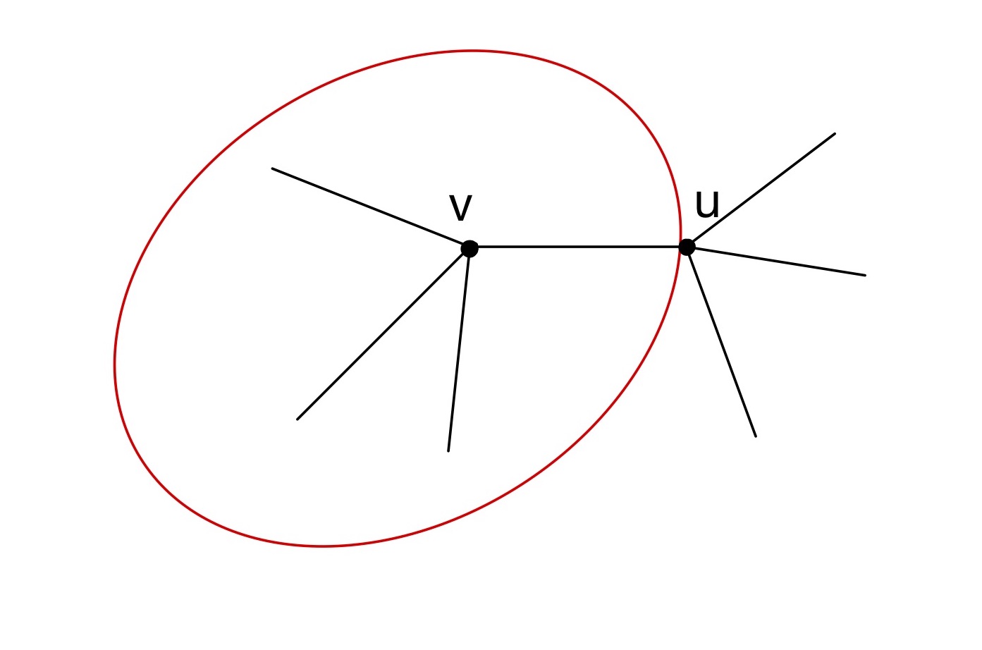
Figure 1. A graph with two internal vertices

References

[1]M. Barlow, K. Burdzy, H. Kaspi, and A. Mandelbaum, Variably Skewed
Brownian Motion, Electronic Communications in Probability, 5 (2000), pp. 57
– 66.
[2]M. Barlow, J. Pitman, and M. Yor, On Walsh’s Brownian motions,
in Séminaire de Probabilités, XXIII, vol. 1372 of Lecture Notes
in Math., Springer, Berlin, 1989, pp. 275–293.
[3]E. Bayraktar and X. Zhang, Embedding of walsh brownian motion,
Stochastic processes and their applications, 134 (2021), pp. 1–28.
[4]R. M. Blumenthal, Excursions of Markov processes, Probability and
its Applications, Birkhäuser Boston, Inc., Boston, MA, 1992.
[5]A. N. Borodin and P. Salminen, Handbook of Brownian motion: facts
and formulae, Springer, 2002.
[6]R. Cairoli and R. C. Dalang, Sequential stochastic optimization,
Wiley Series in Probability and Statistics, Wiley, 1st ed. ed., 2011.
[7]M. Freidlin and S.-J. Sheu, Diffusion processes on graphs:
stochastic differential equations, large deviation principle, Probab. Theory
Related Fields, 116 (2000), pp. 181–220.
[8]M. I. Freidlin and A. D. Wentzell, Diffusion processes on graphs and
the averaging principle, Ann. Probab., 21 (1993), pp. 2215–2245.
[9]E. Hernández-Lemus, Random fields in physics, biology and data
science, Frontiers in Physics, 9 (2021).
[10]T. Ichiba, I. Karatzas, V. Prokaj, and M. Yan, Stochastic integral
equations for Walsh semimartingales, Ann. Inst. Henri Poincaré Probab.
Stat., 54 (2018), pp. 726–756.
[11]T. Ichiba and A. Sarantsev, Stationary distributions and
convergence for Walsh diffusions, Bernoulli, 25 (2019), pp. 2439 – 2478.
[12]T. Ichiba and A. Sarantsev, Stationary distributions and convergence
for Walsh diffusions, Bernoulli, 25 (2019), pp. 2439–2478.
[13]O. Kallenberg, Foundations of modern probability, vol. 99 of
Probability Theory and Stochastic Modelling, Springer, 2021.
Third edition.
[14]I. Karatzas and M. Yan, Semimartingales on rays, walsh diffusions,
and related problems of control and stopping, Stochastic Processes and their
Applications, 129 (2019), pp. 1921 – 1963.
[15]H. Kaspi and A. Mandelbaum, Multi-armed bandits in discrete and
continuous time, The Annals of Applied Probability, 8 (1998), pp. 1270 –
1290.
[16]D. Khoshnevisan, Multiparameter Processes: An Introduction to Random
Fields, Springer Monographs in Mathematics, Springer New York, 2006.
[17]V. Kostrykin, J. Potthoff, and R. Schrader, Brownian motions on
metric graphs, Journal of Mathematical Physics, 53 (2012), p. 095206.
[18]A. Lejay, On the constructions of the skew Brownian motion,
Probability Surveys, 3 (2006), pp. 413 – 466.
[19]A. Mandelbaum, Continuous multi-armed bandits and multiparameter
processes, Ann. Probab., 15 (1987), pp. 1527–1556.
[20]D. Revuz and M. Yor, Continuous martingales and Brownian motion,
vol. 293 of Grundlehren der mathematischen Wissenschaften [Fundamental
Principles of Mathematical Sciences], Springer-Verlag, Berlin, third ed.,
1999.
[21]L. C. G. Rogers, Itô excursion theory via resolvents, Z.
Wahrsch. Verw. Gebiete, 63 (1983), pp. 237–255.
[22]T. S. Salisbury, Construction of right processes from excursions,
Probab. Theory Related Fields, 73 (1986), pp. 351–367.
[23]B. Tsirelson, Triple points: from non-Brownian filtrations to
harmonic measures, Geom. Funct. Anal., 7 (1997), pp. 1096–1142.
[24]V. A. Volkonskii, Random substitution of time in strong markov
processes, Theory of probability and its applications, 3 (1958),
pp. 310–326.
[25]J. B. Walsh, A diffusion with a discontinuous local time, in Temps
locaux, no. 52-53 in Astérisque, Société mathématique de France,
1978, pp. 37–45.