Vacuum stability and scalar masses in the superweak extension of the standard model

Abstract

We study the allowed parameter space of the scalar sector in the superweak extension of the standard model (SM). The allowed region is defined by the conditions of (i) stability of the vacuum and (ii) perturbativity up to the Planck scale, (iii) the pole mass of the Higgs boson falls into its experimentally measured range. We employ renormalization group equations and quantum corrections at two-loop accuracy. We study the dependence on the Yukawa couplings of the sterile neutrinos at selected values. We also check the exclusion limit set by the precise measurement of the mass of the $W$ boson. Our method for constraining the parameter space using two-loop predictions can also be applied to simpler models such as the singlet scalar extension of the SM in a straightforward way.

I Introduction

Currently particle physics is in a similar situation as physics was about 120 years ago. Its standard model (SM) can explain successfully most of the low and high energy phenomena and provide predictions that are in agreement with measurements at high precision. Nevertheless, there are also a handful of outstanding observations that cannot be predicted by the standard model and point towards beyond the standard model (BSM) physics. These unexplained facts are (i) the non-vanishing neutrino masses and mixing matrix elements [1, 2], (ii) the metastable vacuum of the standard model [3, 4], (iii) the need for lepto- and/or baryogenesis to explain baryon asymmetry, i.e. our obvious existence, (iv) the existence of dark matter in the Universe [5, 6, 7, 8, 9], and also (v) the existence of dark energy in the Universe [5]. In addition there is general consensus about the occurrence of cosmic inflation in the early Universe, which also calls for an explanation. There are other observations in particle physics that have almost reached the status of discoveries. Most prominently the prediction of the standard model for the anomalous magnetic moment $a_{\mu}$ of the muon [10] is smaller than the result of the measurement [11, 12] by 4.2 standard deviations. In this case however, the status of the theory is controversial because the evaluation of the hadronic contribution to $a_{\mu}$ requires non-perturbative approach, and the result depends on the method [10, 13]. The resolution of this discrepancy calls for an independent evaluation of this hadronic vacuum polarization contribution before discovery can be claimed.

Some of the observations (i–v) should find understanding in particle physics models, while others may have cosmological origins. Nevertheless, the intimate relation between particle physics and the early Universe, originating from the universal expansion of space-time, gives a strong support for searching answers within particle physics by extending the SM. Such extensions can be put into three categories: (a) ultraviolet complete models from theoretical motivations, such as supersymmetric models; (b) effective field theories like the standard model effective field theory (SMEFT); (c) simplified models that focus on a subset of open questions. This third category includes the dark photon models (gauge extension, see e.g. Refs. [14, 15]), the singlet scalar extensions (see e.g. Refs. [16, 17, 18]) and the introduction of neutrino mass matrices with some variant of the see-saw mechanism, such as in Ref. [19].

The UV complete supersymmetric extensions of the SM are very attractive for solving theoretical issues, but they are becoming less favored by the results of the LHC experiments [20, 21]. Effective field theories proved to be very useful in the past. However, the SMEFT contains 2499 dimension six operators [22], which makes it rather difficult to study experimentally. The simplified models on the other end contain only few new parameters, hence are very attractive from the experimental point of view. However, being simplified models, those cannot give answers to all observations pointing towards BSM physics simultaneously.

In this paper we study a simple UV complete BSM extension along the principles of the SM itself: a renormalizable gauge theory that adds one layer of interactions below the hierarchic layers of the strong, electromagnetic and weak forces, which is called superweak (SW) force [23], mediated by a new U(1) gauge boson $Z^{\prime}$, see Fig. 1. In order to explain the origin of neutrino masses, the field content is enhanced by three generations of right-handed neutrinos. The new gauge symmetry is broken spontaneously by the vacuum expectation value of a new complex scalar singlet. According to exploratory studies, the superweak extension of the standard model (SWSM) has the potential to explain the origin of (i) neutrino masses and mixing matrix elements [24], (ii) dark matter [25], (iii) cosmic inflation [26], (iv) stabilization of the electroweak vacuum [26] and possibly (v) leptogenesis (under investigation).

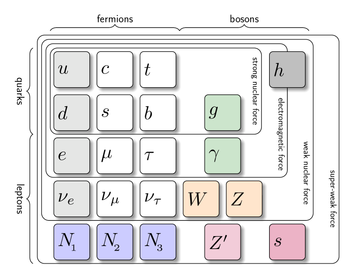
Figure 1: The standard model particle sheet with the superweak extension. The forces act on all particles within the respective box

While these findings are promising, more refined analyses are needed in order to explore the viability of the model. The main motivation of our work is not to prove that the SWSM is the correct description of the fundamental interactions, but rather to check if questions (i–v) listed above can be answered within a single model with as few new parameters as possible. In this paper we revisit the study of the parameter space of the scalar sector of the SWSM as allowed by the requirement of the stability of the vacuum. We improve significantly on our previous analysis [26] in two respects. Firstly, we use renormalization group equations (RGEs) containing the beta functions at two-loop order. More importantly, we take into account both the radiative corrections up to two-loop accuracy and the measured physical values and uncertainties of the parameters of the scalar sector as constraints. A similar study has been performed earlier in the simplified model of single real scalar extension of the SM in Ref. [18]. The important difference between the present work and that analysis is that we include the effect of the right-handed neutrinos in the running of the couplings, which constrains the parameter space further. The inclusion of the two-loop effects is also for the first time in the present work.

II Superweak model

The SWSM is a gauged U(1) extension of the standard model with an additional complex scalar field $\chi$ and three families of sterile neutrinos $\nu_{\mathrm{R},i}$. The model was defined in Ref. [23] and further details on the new sectors were presented in Refs. [26, 24]. Here we recall some details relevant to the present analysis.

The anomaly free charge assignment is shown in Table 1. In particular, the $\chi$ field does not couple directly to any fields of the SM.

Table 1: Group representations and charges of the fermions and scalars in the SWSM

field	SU(3)c	SU(2)L	U(1)Y	U(1)z
$Q_{\mathrm{L}}$	3	2	$\frac{1}{6}$	$\frac{1}{6}$
$u_{\mathrm{R}}$	3	1	$\frac{2}{3}$	$\frac{7}{6}$
$d_{\mathrm{R}}$	3	1	$-\frac{1}{3}$	$-\frac{5}{6}$
$L_{\mathrm{L}}$	1	2	$-\frac{1}{2}$	$-\frac{1}{2}$
$\ell_{\mathrm{R}}$	1	1	$-1$	$-\frac{3}{2}$
$N_{\mathrm{R}}$	1	1	$0$	$\frac{1}{2}$
$\phi$	1	2	$\frac{1}{2}$	1
$\chi$	1	1	$0$	$-1$

After spontaneous symmetry breaking (SSB), we parametrize the SM scalar doublet $\phi$ and the new scalar field as

$$\phi=\frac{1}{\sqrt{2}}\begin{pmatrix}-\mathrm{i}\sqrt{2}\sigma^{+}\\ v+H+\mathrm{i}\sigma_{\phi}\end{pmatrix},\quad\text{and}\quad\chi=\frac{1}{\sqrt{2}}\bigl{(}w+S+\mathrm{i}\sigma_{\chi}\bigr{)}$$ (1)

where $v$ and $w$ are the two vacuum expectation values (VEVs), $H$ and $S$ are two real, scalar fields and $\sigma^{+}$, $\sigma_{\phi/\chi}$ are charged and neutral Goldstone bosons. In terms of these fields the scalar potential in the SWSM is given by

$$V(\phi,\chi)=V_{0}-\mu_{\phi}^{2}|\phi|^{2}-\mu_{\chi}^{2}|\chi|^{2}+\lambda_{\phi}|\phi|^{4}+\lambda_{\chi}|\chi|^{4}+\lambda|\phi|^{2}|\chi|^{2}\,.$$ (2)

The constant $V_{0}$ is irrelevant in our considerations, so we set it to zero in the rest of the paper. Substituting the parametrization (1) into (2), we obtain the tree-level (effective) potential

$$V(H,S)=-\frac{1}{2}\Big{(}\mu_{\phi}^{2}H^{2}+\mu_{\chi}^{2}S^{2}\Big{)}+\frac{1}{4}\Big{(}\lambda_{\phi}H^{4}+\lambda_{\chi}S^{4}+\lambda~{}H^{2}S^{2}\Big{)}$$ (3)

of the real scalar fields. The VEVs are determined by the tadpole equations:

$$\begin{split}\frac{\partial V}{\partial H}\biggl{|}_{H=v,S=w}=0&=v\biggl{(}-\mu_{\phi}^{2}+\frac{1}{2}\lambda w^{2}+\lambda_{\phi}v^{2}\biggr{)},\\ \frac{\partial V}{\partial S}\biggl{|}_{H=v,S=w}=0&=w\biggl{(}-\mu_{\chi}^{2}+\frac{1}{2}\lambda v^{2}+\lambda_{\chi}w^{2}\biggr{)}\,.\end{split}$$ (4)

The mass matrix of the scalar fields is given by the Hessian:

$$\textbf{M}_{\mathrm{s}}^{2}=\begin{pmatrix}\frac{\partial^{2}V}{\partial H^{2}}&\frac{\partial^{2}V}{\partial H\,\partial S}\\ \frac{\partial^{2}V}{\partial S\,\partial H}&\frac{\partial^{2}V}{\partial S^{2}}\end{pmatrix}_{H=v,S=w}=\begin{pmatrix}2\lambda_{\phi}v^{2}&\lambda vw\\ \lambda vw&2\lambda_{\chi}w^{2}\end{pmatrix}\,,$$ (5)

which can be diagonalized by a rotation matrix

$$\mathbf{Z}_{\mathrm{s}}=\begin{pmatrix}\cos\theta_{\mathrm{s}}&\sin\theta_{\mathrm{s}}\\ -\sin\theta_{\mathrm{s}}&\cos\theta_{\mathrm{s}}\end{pmatrix},$$ (6)

so that $\mathbf{Z}_{\mathrm{s}}^{T}\textbf{M}_{\mathrm{s}}^{2}\mathbf{Z}_{\mathrm{s}}=\text{diag}({M}_{h}^{2},{M}_{s}^{2})$. The parameters ${M}_{h}$ and ${M}_{s}$ are the masses of the propagating states $h$ and $s$ . The positivity condition for the masses implies the condition

$$(4\lambda_{\chi}\lambda_{\phi}-\lambda^{2})v^{2}w^{2}>0$$ (7)

among the scalar couplings and VEVs. Explicitly, the angle of rotation and the scalar masses ${M}_{h}$ and ${M}_{s}$ can be expressed through the VEVs and couplings at tree level as

$$\tan(2\theta_{\mathrm{s}}) = \frac{\lambda vw}{\lambda_{\chi}w^{2}-\lambda_{\phi}v^{2}},$$ (8)

$${M}_{h}^{2} = \lambda_{\phi}v^{2}+\lambda_{\chi}w^{2}-\frac{\lambda_{\chi}w^{2}-\lambda_{\phi}v^{2}}{\cos(2\theta_{\mathrm{s}})}\,\,,$$ (9)

$${M}_{s}^{2} = \lambda_{\phi}v^{2}+\lambda_{\chi}w^{2}+\frac{\lambda_{\chi}w^{2}-\lambda_{\phi}v^{2}}{\cos(2\theta_{\mathrm{s}})}\,.$$ (10)

In the absence of mixing ($\lambda=0$, $\theta_{\mathrm{s}}=0$) we have ${M}_{h}=\sqrt{2\lambda_{\phi}v^{2}}$, ${M}_{s}=\sqrt{2\lambda_{\chi}w^{2}}$. As the scalar fields are coupled to the $W^{\pm}$ bosons with the interaction vertices

$$\Gamma_{hWW}^{\mu\nu}=\frac{\mathrm{i}}{2}\biggl{(}g_{\mathrm{L}}^{2}v\cos\theta_{\mathrm{s}}\biggr{)}g^{\mu\nu}\,,\quad\text{and}\quad\Gamma_{sWW}^{\mu\nu}=\frac{\mathrm{i}}{2}\biggl{(}g_{\mathrm{L}}^{2}v\sin\theta_{\mathrm{s}}\biggr{)}g^{\mu\nu}\,,$$ (11)

only the BEH field is coupled to the $W$ bosons and to the other SM fields in the limit of vanishing mixing between the scalars. Hence, we naturally identify the VEV $v$ as that related to the Fermi coupling and also the parameter ${M}_{h}$ with the mass of the Higgs boson measured at the LHC [28] by introducing the notation

$$m_{h}=125.10\,\mathrm{GeV},\quad\Delta m_{h}=0.14\,\mathrm{GeV}\quad\text{and}\quad v=\Big{(}\sqrt{2}G_{\mathrm{F}}\Big{)}^{-1/2}=246.22\,\mathrm{GeV}\,,$$ (12)

and requiring ${M}_{h}\in[m_{h}-\Delta m_{h},m_{h}+\Delta m_{h}]$. In accordance with this assumption, we restrict $\theta_{\mathrm{s}}$ to fall in the range $(-\pi/4,\pi/4)$.

The VEV $w$ can be expressed through these known parameters and the scalar couplings using Eqs. (8) and (9),

$$w={M}_{h}\sqrt{\frac{{M}_{h}^{2}-2\lambda_{\phi}v^{2}}{2\lambda_{\chi}\bigl{(}{M}_{h}^{2}-2\lambda_{\phi}v^{2}\bigr{)}+\lambda^{2}v^{2}}}\,.$$ (13)

Thus, the formal conditions for the non-vanishing $w$, required at the electroweak scale are either

$${M}_{h}^{2}>2\lambda_{\phi}v^{2}\,,\quad\text{with}\quad 4\lambda_{\chi}\lambda_{\phi}>\lambda^{2}$$ (14)

(the second condition deriving from the positivity constraint in (7) for positive $v^{2}w^{2}$), or

$$4\lambda_{\chi}\biggl{(}\lambda_{\phi}-\frac{1}{2}\frac{{M}_{h}^{2}}{v^{2}}\biggr{)}>\lambda^{2}\,,\quad\text{if}\quad 2\lambda_{\phi}v^{2}>{M}_{h}^{2}>0\,.$$ (15)

As we have fixed $v$ and ${M}_{h}$ experimentally, the input value of $\lambda_{\phi}$ decides which of these two cases are to be considered.

Eqs. (3)–(5) are valid at tree level. The effect of the quantum corrections can be summarized by substituting the potential $V$ with the effective potential ${V}_{\rm eff}$, whose formal loop expansion is.

$${V}_{\rm eff}=\sum_{i=0}^{\infty}{V}_{\rm eff}^{(i)}$$ (16)

where ${V}_{\rm eff}^{(0)}=V$ and ${V}_{\rm eff}^{(i)}$ represents the $i$-loop correction.

III Vacuum stability in the SWSM at one-loop accuracy

The potential (3) is stable if it is bounded from below. Due to its continuity in the field variables, it is sufficient to study the positivity of (3) for large values of $h$ and $s$, which translates to the following conditions on the quartic scalar couplings:

$$\begin{split}\lambda_{\phi},\lambda_{\chi}&>0\,,\\ 4\lambda_{\phi}\lambda_{\chi}-\lambda^{2}&>0\quad\mbox{for}\quad\lambda<0\,.\end{split}$$ (17)

Taking into account the radiative corrections leads to (i) dependence on the renormalization scale $\mu$ for all renormalized couplings and (ii) the corrections ${V}_{\rm eff}^{(i)}$. While it is straightforward to require that the conditions (17) be satisfied for the running couplings at any sensible value of $\mu$, we cannot write the stability conditions for the one-loop effective potential in a closed form such as in Eq. (17) valid at tree level. Instead, we take an alternative path by requiring the existence of a non-vanishing $w({M}_{\rm t})$ indirectly, extracting it from the known pole mass of the Higgs boson, rather than computing it explicitly form the effective potential (16) with radiative corrections taken into account. Our procedure can be described in terms of analytic expressions at the one-loop accuracy as follows.

We investigate the vacuum stability in the range $\mu\in({M}_{\rm t},{M}_{\rm Pl})$, i.e. from the pole mass ${M}_{\rm t}$ of the t quark up to the Planck mass ${M}_{\rm Pl}$ where quantum gravitational effects become important. The scale dependence of a given coupling $g$ is described by the autonomous system coupled differential equations of the form

$$\frac{\partial g}{\partial t}=\beta_{g}\,,$$ (18)

called RGEs, where $\partial/\partial t=\mu\,\partial/\partial\mu$. We assume that the model remains perturbatively valid for the complete range by requiring

$$|g(\mu)|<4\pi\,,\quad\mu\in({M}_{\rm t},{M}_{\rm Pl})$$ (19)

for any coupling $g$ in the theory, which we check in the stability analysis. Consequently, we can employ perturbation theory to compute the $\beta_{g}$ functions. We integrate the complete set of RGEs of the SWSM, while requiring the stability and perturbativity conditions (17) and (19). We also assume the existence of $w$ at the scale $\mu={M}_{\rm t}$, which implies the existence of a second massive neutral gauge boson and a second massive scalar particle as predictions of the model. To check this condition, we compute the loop corrected scalar mixing angle and scalar pole masses:

$$\tan\bigl{(}2\theta_{\mathrm{s}}(p^{2})\bigr{)}=\frac{\lambda(\mu)v(\mu)w(\mu)+\Pi_{HS}(p^{2})}{\lambda_{\chi}(\mu)w(\mu)^{2}-\lambda_{\phi}(\mu)v(\mu)^{2}+\Pi_{-}(p^{2})},$$ (20)

$${M}_{h}^{2}=\lambda_{\phi}(\mu)v(\mu)^{2}+\lambda_{\chi}(\mu)w(\mu)^{2}+\Pi_{+}({M}_{h}^{2})-\frac{\lambda_{\chi}(\mu)w(\mu)^{2}-\lambda_{\phi}(\mu)v(\mu)^{2}+\Pi_{-}({M}_{h}^{2})}{\cos\bigl{(}2\theta_{\mathrm{s}}({M}_{h}^{2})\bigr{)}}\,,$$ (21)

$${M}_{s}^{2}=\lambda_{\phi}(\mu)v(\mu)^{2}+\lambda_{\chi}(\mu)w(\mu)^{2}+\Pi_{+}({M}_{s}^{2})+\frac{\lambda_{\chi}(\mu)w(\mu)^{2}-\lambda_{\phi}(\mu)v(\mu)^{2}+\Pi_{-}({M}_{s}^{2})}{\cos\bigl{(}2\theta_{\mathrm{s}}({M}_{s}^{2})\bigr{)}}\,,$$ (22)

using the shorthand notation

$$\Pi_{\pm}(p^{2})=\frac{1}{2}\biggl{(}\tilde{\Pi}_{SS}(p^{2})\pm\tilde{\Pi}_{HH}(p^{2})\biggr{)}\,,$$ (23)

where $\tilde{\Pi}_{\varphi\varphi}(p^{2})=\Pi_{\varphi\varphi}(p^{2})-T_{\varphi}/\langle\varphi\rangle$, with $\Pi_{\varphi_{I}\varphi_{J}}(p^{2})$ being the sum of all one particle irreducible (1PI) two-point functions with external legs $\varphi_{I}$ and $\varphi_{J}$, while $T_{\varphi}$ is the sum of all 1PI one-point functions with external leg $\varphi$ ($\varphi$, $\varphi_{I}=H$ or $S$). In other words, Eqs. (20)–(22) are valid at any order in perturbation theory. We collect these one- and two-point functions computed at one-loop accuracy in App. A. As shown explicitly, each coupling and VEV in Eqs. (20)–(22) depends on the renormalization scale $\mu$, but the pole masses ${M}_{h}^{2}$ and ${M}_{s}^{2}$ do not up to the effect of neglected higher order corrections. An important check of our calculations is the independence of the scalar pole masses ${M}_{h}$ and ${M}_{s}$ of the renormalization scale $\mu$

$$\mu\frac{\partial{M}_{h}}{\partial\mu}=\mu\frac{\partial{M}_{s}}{\partial\mu}=0.$$ (24)

As mentioned, we identify the pole mass ${M}_{h}$, computed in perturbation theory in (21) as the observed Higgs boson mass $m_{h}\pm\Delta m_{h}$, which constrains the possible values of $w({M}_{\rm t})$ severely for a given set of input couplings at $\mu={M}_{\rm t}$. The lower panels in Fig. 2 show the dependence of $|\Delta M_{h}|$, with $\Delta M_{h}=M_{h}-m_{h}$, on $w({M}_{\rm t})$. We see that it falls below the experimental uncertainty $\Delta m_{h}$, represented by the dashed lines, in a fairly narrow range of $w({M}_{\rm t})$. To find the range of values of the allowed $w^{(i)}({M}_{\rm t})$, with superscript referring to the accuracy in the perturbative order, we solve the two equations

$${M}_{h}(w^{(1)})\biggr{|}_{\mu={M}_{\rm t}}=m_{h}\pm\Delta m_{h}$$ (25)

for $w^{(1)}({M}_{\rm t})$ numerically. We consider the two solutions physical if those are positive, shown by the vertical lines. Then we use the accepted values $w^{(1)}({M}_{\rm t})$, falling into the ranges between the vertical line, to compute the possible values of ${M}_{s}$ using Eq. (22). This procedure is shown by the plots on the top of Fig. 2 for a specific set of input couplings.

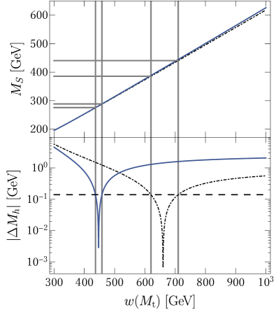
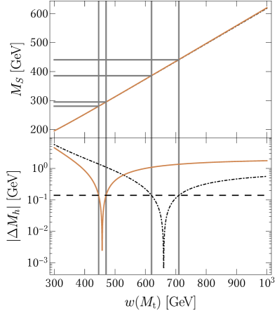
Figure 2: Dependence of the absolute difference ${M}_{h}$ minus the observed Higgs boson mass on $w({M}_{\rm t})$ (bottom) and the dependence of ${M}_{s}$ on $w({M}_{\rm t})$ (top) with input values $\lambda_{\phi}({M}_{\rm t})=0.15$, $\lambda_{\chi}({M}_{\rm t})=0.2$ and $\lambda({M}_{\rm t})=0.1$. Left: $y_{x}({M}_{\rm t})=0$, right: $y_{x}({M}_{\rm t})=0.8$. The dashed horizontal line corresponds to the uncertainty $\Delta m_{h}$. The black dash-dotted curves are computed at tree level (Eqs. (9) and (10)), while the solid colored ones at one loop (Eqs. (21) and (22)).

The complete set of running couplings can be grouped into three sets. The (i) SM couplings $g_{Y},~{}g_{\mathrm{L}},~{}g_{\mathrm{s}},~{}y_{\mathrm{t}}$, the (ii) SW gauge coupling $g_{z}$ and (iii) the scalar quartic couplings $\lambda_{\phi},\lambda_{\chi},\lambda$ together with the sterile neutrino Yukawa coupling $y_{x}$. We assume one light sterile neutrino – a candidate for dark matter [25] – and two heavy ones with equal masses for simplicity, $y_{x}=y_{x,5}=y_{x,6}$. We neglect the effect of the SW gauge coupling from our analysis because its maximally allowed value is very small, $g_{z}\lesssim 10^{-4}$, if the model is to explain the origin of dark matter [25] and also should obey the direct observational limit of the NA61 experiment [29]. Explicitly, in group (iii) we have the following autonomous system of RGEs at one loop:

$$\begin{split}\frac{\partial\lambda_{\phi}}{\partial t}&=\beta_{\lambda_{\phi},\text{SM}}^{(1)}+\frac{\lambda^{2}}{(4\pi)^{2}}\,,\quad\frac{\partial\lambda_{\chi}}{\partial t}=\frac{1}{(4\pi)^{2}}\biggl{(}20\lambda_{\chi}^{2}+2\lambda^{2}-2y_{x}^{4}+4\lambda_{\chi}y_{x}^{2}\biggr{)},\\ \frac{\partial\lambda}{\partial t}&=\frac{\lambda}{(4\pi)^{2}}\biggl{(}-\frac{3}{2}g_{Y}^{2}-\frac{9}{2}g_{\mathrm{L}}^{2}+12\lambda_{\phi}+8\lambda_{\chi}+4\lambda+6y_{t}^{2}+2y_{x}^{2}\biggr{)},\end{split}$$ (26)

for the scalar couplings, with $\beta_{\lambda_{\phi},\text{SM}}^{(1)}$ being the one-loop beta function of the SM quartic scalar coupling, and

$$\frac{\partial y_{x}}{\partial t}=\frac{2y_{x}^{3}}{(4\pi)^{2}}\,,\qquad\frac{\partial w}{\partial t}=-\frac{w}{(4\pi)^{2}}\frac{y_{x}^{2}}{2}$$ (27)

for the Yukawa coupling and new VEV. The one-loop beta functions show, that a sufficiently large Higgs portal coupling $\lambda$ is able to drive $\lambda_{\phi}$ and $\lambda_{\chi}$ to positive values, while the sterile neutrino Yukawa couplings drive $\lambda_{\chi}$ towards negative values. The last equation, the RGE for $w$ does not affect the vacuum stability analysis. We present it as it is used in checking the conditions in Eq. (24).

There are three SM precision parameters measured precisely, $G_{\mathrm{F}},~{}{M}_{Z}$ and $\alpha_{\text{em}}^{\overline{\text{MS}}}({M}_{Z})$, which can be turned into input values for the couplings in group (i) together with the less precisely known ${M}_{\rm t}$ and $\alpha_{\mathrm{s}}^{\overline{\text{MS}}}({M}_{Z})$. The self energies $\Pi_{WW}(p^{2})$ and $\Pi_{ZZ}(p^{2})$ also receive contributions $\Pi^{\text{SW}}_{VV}(p^{2})$ due to the SW extension, given in Eq. (40), which shift the input values of the VEV $v$ and the electroweak gauge couplings. Hence, we use the following inputs in group (i)

$$\begin{split}g_{Y}({M}_{\rm t})&=0.3586+\delta g_{Y}({M}_{\rm t}),\\ g_{\mathrm{L}}({M}_{\rm t})&=0.6477+\delta g_{\mathrm{L}}({M}_{\rm t}),\\ v({M}_{\rm t})&=247.55~{}\mathrm{GeV}+\delta v({M}_{\rm t}),\end{split}$$ (28)

with $g_{\mathrm{s}}({M}_{\rm t})=1.167$ and $y_{\mathrm{t}}({M}_{\rm t})=0.940$. The SW corrections $\delta g_{Y},\delta g_{\mathrm{L}}$ and $\delta v$ are defined in App. B. The SM value of the gauge and scale dependent VEV $v$ in the Feynman gauge is $v_{\text{SM}}({M}_{\rm t})=247.55~{}\mathrm{GeV}$. The SW corrections to the electroweak input parameters $\delta g_{Y}$, $\delta g_{\mathrm{L}}$ and $\delta v$ are small and do not modify noticably our final results even at two loops. We take the value of $y_{\mathrm{t}}({M}_{\rm t})$ from the fit formula (25) of Ref. [4] as the largest possible value. This choice is the most conservative one concerning the vacuum stability because the main culprit causing the metastable SM vacuum is the large value of the t quark Yukawa coupling $y_{t}({M}_{\rm t})$. The last set (iii) of the input couplings are unconstrained and we scan their values at $\mu={M}_{\rm t}$ in order to obtain the parameter space in $\{\lambda_{\phi},\lambda_{\chi},\lambda,y_{x}\}_{\mu={M}_{\rm t}}$ where the stability (17), perturbativity (19) conditions in the range $\mu\in({M}_{\rm t},{M}_{\rm Pl})$, together with existence of the $w$ vacuum at $\mu={M}_{\rm t}$ are fulfilled.

We have scanned the volume $V_{\lambda}(y_{x})=\{\lambda_{\phi},\lambda_{\chi},\lambda\}_{\mu={M}_{\rm t}}$ spanned by the input couplings at fixed values of $y_{x}({M}_{\rm t})$ to find the parameter space allowed by our conditions. There are two quantitatively different regions. In the first one (a) ${M}_{s}<{M}_{h}$, i.e. the new scalar is lighter than the Higgs boson, whereas in the second one (b) ${M}_{s}>{M}_{h}$. We shall present the result of such scans in the next section where we the computations will be performed at two-loop accuracy. Having found the allowed region of the input parameters, we can compute the scalar mixing angle and mass of the new scalar using Eqs. (20) and (22), to obtain the allowed parameter space in the ${M}_{s}-|\sin(\theta_{\mathrm{s}}({M}_{\rm t}))|$ plane, shown in Fig. 3 at selected values of the neutrino Yukawa coupling. In case (a), the parameter space is empty for $y_{x}({M}_{\rm t})=0$, but it grows non-linearly with increasing $y_{x}({M}_{\rm t})$. For instance, the parameter space for $y_{x}({M}_{\rm t})=0.4$ is not empty, but still invisible at the resolution of Fig. 3, as in that case one has ${M}_{s}<300\,\mathrm{MeV}$ and $|\sin(\theta_{\mathrm{s}})|<0.04$. For $y_{x}({M}_{\rm t})\gtrsim 1$ the stability condition $\lambda_{\chi}>0$ is not satisfied at any scale below ${M}_{\rm Pl}$. It turns out that in case (b) the value of the VEV $w^{(1)}({M}_{\rm t})$ and hence that of ${M}_{s}$ can be larger than shown in the plot when the scalar mixing coupling tends to zero. As that also means vanishing mixing coupling $\lambda$, it represents the phenomenologically rather irrelevant case of very weakly coupled dark sector.

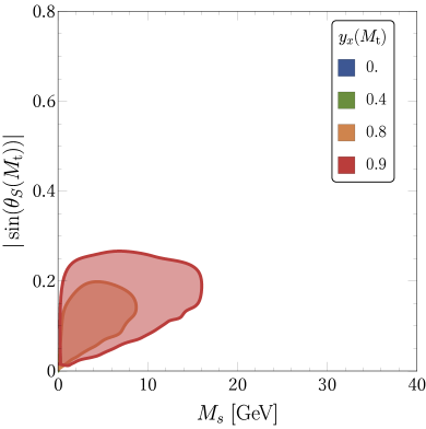
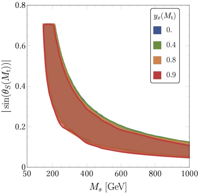
Figure 3: Allowed parameter space $V_{\lambda}(y_{x})$ in the ${M}_{s}-|\sin(\Theta_{S})|$ plane at representative values of $y_{x}$ at one loop accuracy. The different colored areas correspond to different values of $y_{x}({M}_{\rm t})$ as shown in the legends. Left: ${M}_{s}<{M}_{h}$, right: ${M}_{s}>{M}_{h}$.

IV Vacuum stability in the SWSM at two-loop accuracy

In order to check the robustness of the perturbative analysis of the parameter space where the vacuum is stable, we have repeated the procedure described in the previous section at two-loop accuracy. Given a set of input couplings $\{\lambda_{\phi}({M}_{\rm t}),\lambda_{\chi}({M}_{\rm t}),\lambda({M}_{\rm t}),y_{x}({M}_{\rm t})\}$, we first computed $w^{(1)}({M}_{\rm t})$ at $\mu={M}_{\rm t}$, using our analytic formulae as described in the previous section. We solved the two-loop $\beta$-functions to check the conditions of stability and perturbativity only if we found $w^{(1)}({M}_{\rm t})>0$. If all the stability and perturbativity conditions were fulfilled for the input values $\{\lambda_{\phi}({M}_{\rm t}),\lambda_{\chi}({M}_{\rm t}),\lambda({M}_{\rm t}),y_{x}({M}_{\rm t})\}$, we used SPheno [30, 31] to compute the scalar pole masses at two-loops, ${M}_{h}^{(2)}$ and ${M}_{s}^{(2)}$, using $w$ as a free input parameter. Starting from the initial value $w=w^{(1)}({M}_{\rm t})$, we searched for the $w$ at which

$${M}_{h}^{(2)}(w)=m_{h}\,,$$ (29)

which we call $w=w^{(2)}$. This procedure of starting with using only such points in the parameter space where the condition $w^{(1)}({M}_{\rm t})>0$ is satisfied saves significant CPU time as the numerical solution of the two-loop $\beta$-functions and especially the computations in SPheno are very time consuming .

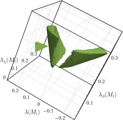
Figure 4: Three dimensional parameter space at $y_{x}({M}_{\rm t})=0.4$.

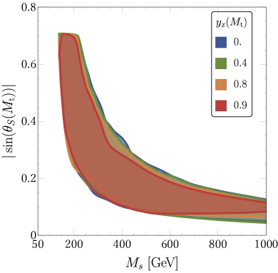
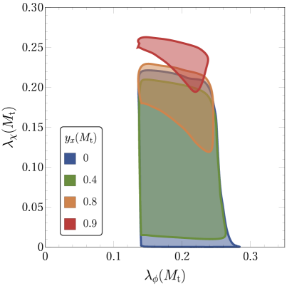
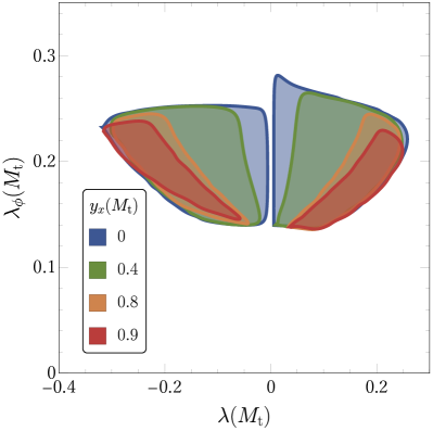
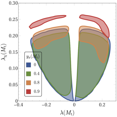
Figure 5: Planar projections of the allowed parameter space, where ${M}_{s}>{M}_{h}$ and the conditions (17), (19), $w^{(2)}({M}_{\rm t})>0$ are fulfilled at two-loop accuracy. Top left: allowed regions in the ${M}_{s}-|\sin\theta_{\mathrm{s}}|$ plane, other plots show the two-dimensional projections of the three-dimensional allowed regions in $V_{\lambda}(y_{x})$. The different colored regions correspond to different values of $y_{x}$ as shown in the legends.

The parameter space is shown by a perspective view at $y_{x}({M}_{\rm t})=0.4$ in Fig. 4, and its projections to the two-dimensional sub-spaces at selected values of $y_{x}({M}_{\rm t})$ in Figs. 5 and 6. We have also computed the regions $V_{\lambda}(y_{x})$ using the tree-level relation (13) instead of the one-loop one in Eq. (21) as done typically in the case of scalar singlet extensions (see e.g. [33]). We found that the allowed region on the ${M}_{s}-|\sin(\theta_{\mathrm{s}})|$ plane for case (a) ${M}_{s}<{M}_{h}$ is sensitive to such a change in an interesting way: for vanishing Yukawa coupling the allowed region found using Eq. (13) disappears at one loop (see the discussion of Fig. 3 in the previous section), but reappears at two loops, which had not been found in pervious analyses. If $y_{x}({M}_{\rm t})$ is increased from zero, we find non-empty parameter space at any of the first three orders in perturbation theory. The minimum value of ${M}_{s}$ in region (a) depends on $y_{x}({M}_{\rm t})$, but it is always larger than about 1 GeV in the two-loop analysis.

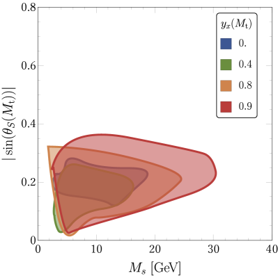
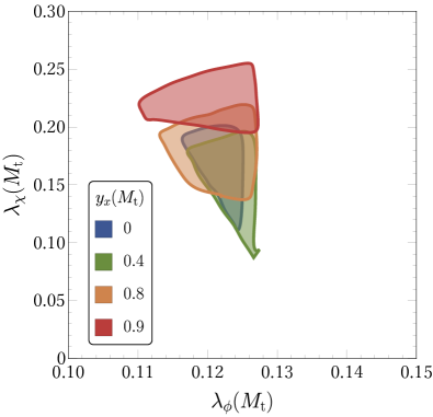
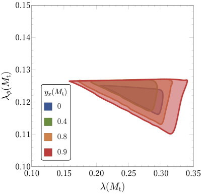
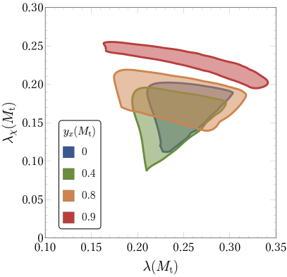
Figure 6: Same as Fig. 5 for ${M}_{s}>{M}_{h}$.

One can make two important remarks about the parameter space in case (b) ${M}_{s}>{M}_{h}$ presented in Fig. 6. On the one hand, the parameter space shrinks as $y_{x}({M}_{\rm t})$ increases and it disappears completely for $y_{x}({M}_{\rm t})\gtrsim 1$. On the other hand, we have $|\lambda({M}_{\rm t})|>0$, because for $\lambda({M}_{\rm t})=0$ the scalar mixing vanishes, and then $\lambda_{\phi}$ coincides with $\lambda_{\rm SM}$, which does not satisfy the vacuum stability conditions, while preserving the pole mass of the Higgs boson. Also, the volume $V_{\lambda}(y_{x})$ increases slightly with increasing order in perturbation theory.

We have checked Eq. (24) numerically for both cases (a) and (b) at randomly selected input values $\{\lambda_{\phi},\lambda_{\chi},\lambda,y_{x}\}_{\mu={M}_{\rm t}}$ in the range $\mu\in\bigl{(}0.5{M}_{\rm t},2{M}_{\rm t}\bigr{)}$ and compared the scale dependences of the tree level masses (9) and (10) to the scale dependences of the one-loop accurate pole masses (21) and (22). As shown in Fig. 7, we have found that the scale dependences of the tree level masses are reduced significantly at one-loop and even more at two-loop accuracy. The sizeable difference between the scalar pole masses ${M}_{s}$ at the first two orders of perturbation theory (and to much less extent between the next two orders) are not caused by radiative corrections. Rather than loop corrections to the masses, the jumps originate from the shifts in $w({M}_{\rm t})$ required to reproduce Higgs boson pole mass at different orders of perturbation theory, as can be seen in Fig. 2.

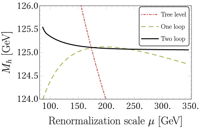
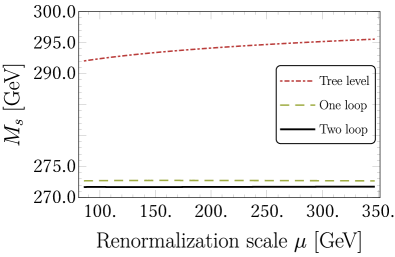
Figure 7: Dependencees of the scalar boson masses ${M}_{h}^{(i)}$ and ${M}_{s}$ on the renormalization scale $\mu$ in the range $(0.5{M}_{\rm t},2{M}_{\rm t})$ at different orders of the perturbation theory at $y_{x}({M}_{\rm t})=0.4$, $\lambda_{\phi}({M}_{\rm t})=0.241$, $\lambda_{\chi}({M}_{\rm t})=0.096$, $\lambda({M}_{\rm t})=0.217$.

The theoretical prediction for the $W$-boson mass uses precision electroweak observables (except ${M}_{W}$ itself) and it is sensitive to new physics [34]. Hence, it is often used as a benchmark compared to the experimentally observed value [28]

$$M_{W}^{\text{exp.}}=80.379\pm 0.012\,\mathrm{GeV}\,.$$ (30)

The current, most precise theoretical estimates are $M_{W}^{\text{theo.}}=80.359\pm 0.011\,\mathrm{GeV}$ [35], $80.362\pm 0.007\,\mathrm{GeV}$ [36] and $80.357\pm 0.009\pm 0.003\,\mathrm{GeV}$ [37]. We take 80.360 GeV as SM prediction and the combined uncertainty from the experimental and theoretical values to be $\Delta{M}_{W}\simeq 17\,\mathrm{MeV}$. We set twice this value as an upper limit to find the allowed range for the new physics contribution to $M_{W}^{\text{theo.}}$, which means that the SW contribution to the mass of the $W$ boson is excluded outside the range $(19\pm 34)$ MeV, i.e outside $[-15,53]$ MeV.

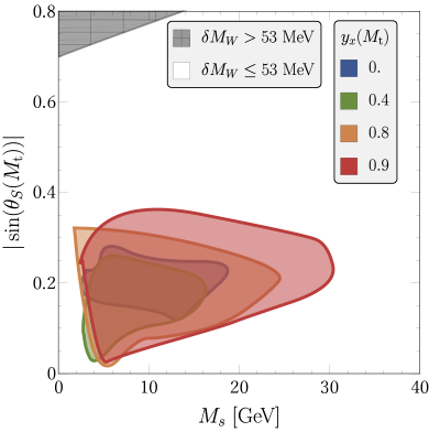
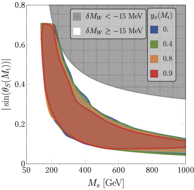
Figure 8: Allowed parameter space in the ${M}_{s}-|\sin(\Theta_{S})|$ plane at representative values of $y_{x}$ at two-loop accuracy. The region with a gray grid represents the portion of the parameter space where $\delta{M}_{W}$, i.e. the radiative corrections in the SWSM to the $W$-boson mass exceed the value given in the plot legend.

We computed the SW contributions $\delta{M}_{W}^{\rm SW}$ to $M_{W}^{\text{theo.}}$ at one loop accuracy. We found, that the contribution of the new gauge sector is heavily suppressed due to the required smallness of the new gauge coupling $g_{z}\lesssim 10^{-4}$. The sterile neutrinos may change the measured value of the Fermi coupling $G_{\mathrm{F}}$ affecting the mass of the $W$ boson already at tree level [38]. As a matter of fact right-handed neutrinos can provide significant contribution to the $W$ boson mass [39], although at the price of introducing some tension with universality bounds. Hence, a proper account of the effect of sterile neutrinos is certainly warranted, but it is beyond the scope of the present paper and we leave it for a planned global scan of the parameter space. The contribution of the new scalar sector to ${M}_{W}$ however, can be comparable to $\Delta{M}_{W}$ [40, 34]. We present the SW correction $\delta{M}_{W}$ in (46) of App. B, expressed with two free parameters, ${M}_{s}$ and $\sin^{2}\theta_{\mathrm{s}}$. For the case of light new scalar, ${M}_{s}<{M}_{h}$, the SW correction is positve, while for the heavy one it is negative. The excluded regions obtained by (a) $\delta{M}_{W}>53$ MeV and (b) $\delta{M}_{W}<-15$ MeV are presented in Fig. 8 overlayed the region where the new scalar particle is allowed by vacuum stability, perturbativity and precision measurement of the Higgs boson mass. We see that the $W$-mass measurement at present uncertainties does not provide significant reduction of the parameter space. However, if the improved measurement published recently by the CDF collaboration [41] will be confirmed, the stability of the vacuum in the high-mass region becomes incompatible with the CDF-II $W$ mass as in that case the SW correction to the SM value is negative. The low-mass region also becomes significantly constrained. In Fig. 9 we present the allowed parameter space together with contour lines representing the border of the excluded parameter space (below the line) assuming a $\delta{M}_{W}$ increase of the $W$ mass by selected benchmark values due to the new scalar in the self energy loop. Clearly, the large positive shift required to explain the CDF-II result is not compatible with the conditions of stability and perturbativity of the scalar sector of the model.

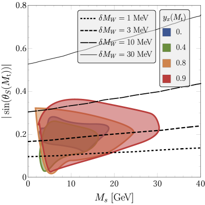
Figure 9: Allowed parameter space in the ${M}_{s}-|\sin(\Theta_{S})|$ plane at representative values of $y_{x}$ at two-loop accuracy for ${M}_{s}>{M}_{h}$. The contours at selective values of $\delta{M}_{W}$ represent the borderline in the parameter space below which the new scalar cannot be solely responsible to the increase of the $W$ boson mass by $\delta{M}_{W}$ with respect to the SM value.

V Conclusions and outlook

In this paper we have scanned the parameter space of the superweak extension of the standard model in order to find the allowed parameter space of the scalar sector where the following assumptions are fulfilled: (i) the vacuum be stable and (ii) the model parameters remain perturbative up to the Planck scale, (iii) the pole mass of the Higgs boson must fall into its experimentally measured range. The first two of these constraints were taken into account in our preliminary work [26]. In this paper we superseed that former study by taking into account the two-loop corrections both in the renormalization group equations of the running couplings as well as the measured value of the mass of the Higgs boson. We have taken into account the largest neutrino Yukawa coupling $y_{x}$. In the limit of vanishing $y_{x}$ and neglecting the superweak gauge coupling, the model essentially reduces to the case of singlet scalar extension of the standard model.

In the two-loop analysis we found a non-empty region in the ${M}_{s}-\sin\theta_{\mathrm{s}}$ parameter space for ${M}_{s}<{M}_{h}$, increasing with $y_{x}$ up to $y_{x}({M}_{\rm t})\simeq 1$ where the condition of stability is not fulfilled any longer. Such a region have been missed in the case of $y_{x}=0$ in earlier analyises of the singlet scalar extension performed only at one-loop accuracy (see e.g. [18]).

Of course, there is a lot of experimental results that also constrain the parameter space. The new physics contributions to electroweak precision observables as well as direct searches for the decay of a scalar particle into standard model ones provide strong constraints. Of those, we have studied only the effect of the experimental result on the mass of the $W$ boson in this paper. We saw that while ${M}_{W}$ can indeed limit the parameter space, the current world average without the new CDF-II result cannot provide further constraint on the parameter space. If we also include the CDF II result in the average – in spite of being incompatible with the previous average –, then the parameter space allowed by our assumptions become incompatible with the $W$-mass constraint. Clearly, it is of utmost importance to take into account all the available experimental constraints, not only from collider experiments, also from neutrino experiments. Such a complete study of the parameter space is beyond the scope of the present paper and we leave it to an upcoming study where we plan to use the analytic expressions of the present work.

Appendix A Loop corrections to the scalar masses in the SWSM

On one hand, the quantum effects correct the tadpole equations (4), such that

$$\begin{split}0&=v\biggl{(}-\mu_{\phi}^{2}+\frac{1}{2}\lambda w^{2}+\lambda_{\phi}v^{2}\biggr{)}+T_{H},\\ 0&=w\biggl{(}-\mu_{\chi}^{2}+\frac{1}{2}\lambda v^{2}+\lambda_{\chi}w^{2}\biggr{)}+T_{S}\,,\end{split}$$ (31)

where $T_{\varphi}$ is the sum of all 1PI one-point functions with external leg $\varphi=H$ or $S$. On the other hand, the scalar self-energies $\Pi_{\varphi_{I}\varphi_{J}}$ – i.e. the sum of all 1PI Feynmann graphs with external legs $\varphi_{I}$ and $\varphi_{J}$ – correct directly the propagator matrix of the scalar fields $H$ and $S$. The inverse-propagator matrix after applying the tadpole equations (31) to eliminate the mass parameters $\mu_{\phi}$ and $\mu_{\chi}$ is given as

$$\begin{pmatrix}p^{2}&0\\ 0&p^{2}\end{pmatrix}-\begin{pmatrix}2\lambda_{\phi}v^{2}+\tilde{\Pi}_{HH}(p^{2})&\lambda vw+\Pi_{SH}(p^{2})\\ \lambda vw+\Pi_{HS}(p^{2})&2\lambda_{\chi}w^{2}+\tilde{\Pi}_{SS}(p^{2})\end{pmatrix},$$ (32)

where $\tilde{\Pi}_{\varphi\varphi}(p^{2})=\Pi_{\varphi\varphi}(p^{2})-T_{\varphi}/\langle\varphi\rangle$ with $\langle\varphi\rangle=v$, $w$. In order to obtain the mixing angle $\theta_{\mathrm{s}}$ (20) and the scalar pole masses (21) and (22), one has to diagonalize the real part of (32), leading to Eqs. (20), (21) and (22).

We have implemented a SARAH model file for the SWSM [24], and used it to compute the one-loop scalar self-energies and tadpoles in Feynman gauge ($\xi=1$). In the following, we list explicitly the one-loop corrections to the scalar inverse-propagator matrix (32), after some simplifications of the SARAH output.

The Higgs self energy is

$$\begin{split}\tilde{\Pi}_{HH}(p^{2})=&\kappa\biggl{\{}3y_{t}^{2}\bigl{(}4m_{t}^{2}-p^{2}\bigr{)}B_{0}\bigl{(}p^{2},m_{t}^{2},m_{t}^{2}\bigr{)}-\frac{1}{2}\lambda^{2}v^{2}B_{0}\bigl{(}p^{2},0,0\bigr{)}\\ &+\frac{\lambda w\sin(2\theta_{\mathrm{s}})}{2v}\biggl{(}A_{0}(m_{s}^{2})-A_{0}(m_{h}^{2})\biggr{)}\\ &-\frac{1}{2}\bigl{(}6\lambda_{\phi}v\cos^{2}\theta_{\mathrm{s}}-\lambda w\sin(2\theta_{\mathrm{s}})+\lambda v\sin^{2}\theta_{\mathrm{s}}\bigr{)}^{2}B_{0}\bigl{(}p^{2},m_{h}^{2},m_{h}^{2}\bigr{)}\\ &-\frac{1}{2}\bigl{(}\lambda v\cos^{2}\theta_{\mathrm{s}}+\lambda w\sin(2\theta_{\mathrm{s}})+6\lambda_{\phi}v\sin^{2}\theta_{\mathrm{s}}\bigr{)}^{2}B_{0}\bigl{(}p^{2},m_{s}^{2},m_{s}^{2}\bigr{)}\\ &-\frac{1}{2}\bigl{(}\lambda w\cos(2\theta_{\mathrm{s}})+(3\lambda_{\phi}-\lambda/2)v\sin(2\theta_{\mathrm{s}})\bigr{)}^{2}B_{0}\bigl{(}p^{2},m_{s}^{2},m_{h}^{2}\bigr{)}\\ &+\frac{1}{v^{2}}\biggl{(}\bigl{(}4p^{2}m_{W}^{2}-12m_{W}^{4}-4\lambda_{\phi}^{2}v^{4}\bigr{)}B_{0}\bigl{(}p^{2},m_{W}^{2},m_{W}^{2}\bigr{)}+8m_{W}^{2}\biggr{)}\\ &+\frac{1}{2v^{2}}\biggl{(}\bigl{(}4p^{2}m_{Z}^{2}-12m_{Z}^{4}-4\lambda_{\phi}^{2}v^{4}\bigr{)}B_{0}\bigl{(}p^{2},m_{Z}^{2},m_{Z}^{2}\bigr{)}+8m_{Z}^{2}\biggr{)}\biggr{\}}\end{split}$$ (33)

where $\kappa=(4\pi)^{-2}$ and $m_{p}(\mu)$ is the running mass of particle $p$ as computed using tree level relations. If the elements of the Dirac neutrino mass matrix $\mathbf{M}_{D}$ are much smaller than those of the Majorana neutrino mass matrix $\mathbf{M}_{N}$, i.e. $\bigl{(}\mathbf{M}_{D}\bigr{)}_{ij}\ll\bigl{(}\mathbf{M}_{N}\bigr{)}_{kk}$ for any $i,j,k\in(1,2,3)$, then the loop correction to the scalar mass from the active neutrinos is negligible and the sterile neutrinos contribute to $\tilde{\Pi}_{SS}$ only, namely

$$\begin{split}\tilde{\Pi}_{SS}(p^{2})=\kappa&\biggl{\{}\frac{1}{2}\sum_{i=1}^{3}y_{x,i}^{2}\bigl{(}4m_{N,i}^{2}-p^{2}\bigr{)}B_{0}\bigl{(}p^{2},m_{N,i}^{2},m_{N,i}^{2}\bigr{)}\\ &+\frac{\lambda v\sin(2\theta_{\mathrm{s}})}{2w}\biggl{(}A_{0}(m_{s}^{2})-A_{0}(m_{h}^{2})\biggr{)}\\ &-\frac{1}{2}\bigl{(}\lambda w\cos^{2}\theta_{\mathrm{s}}-\lambda v\sin(2\theta_{\mathrm{s}})+6\lambda_{\chi}w\sin^{2}\theta_{\mathrm{s}}\bigr{)}^{2}B_{0}\bigl{(}p^{2},m_{h}^{2},m_{h}^{2}\bigr{)}\\ &-\frac{1}{2}\bigl{(}6\lambda_{\chi}w\cos^{2}\theta_{\mathrm{s}}+\lambda v\sin(2\theta_{\mathrm{s}})+\lambda w\sin^{2}\theta_{\mathrm{s}}\bigr{)}^{2}B_{0}\bigl{(}p^{2},m_{s}^{2},m_{s}^{2}\bigr{)}\\ &\quad-\frac{1}{2}\bigl{(}\lambda v\cos(2\theta_{\mathrm{s}})-(3\lambda_{\chi}-\lambda/2)w\sin(2\theta_{\mathrm{s}})\bigr{)}^{2}B_{0}\bigl{(}p^{2},m_{s}^{2},m_{h}^{2}\bigr{)}\\ &-w^{2}\biggl{(}\lambda^{2}B_{0}\bigl{(}p^{2},m_{W}^{2},m_{W}^{2}\bigr{)}+\frac{1}{2}\lambda^{2}B_{0}\bigl{(}p^{2},m_{Z}^{2},m_{Z}^{2}\bigr{)}-2\lambda_{\chi}^{2}B_{0}\bigl{(}p^{2},0,0\bigr{)}\biggr{)}\biggr{\}}\end{split}$$ (34)

and

$$\begin{split}\Pi_{HS}&(p^{2})=\Pi_{SH}(p^{2})=\\ &=\kappa\biggl{\{}\frac{1}{2}\lambda\sin(2\theta_{\mathrm{s}})\biggl{(}A_{0}(m_{h}^{2})-A_{0}(m_{s}^{2})\biggr{)}\\ &+\frac{1}{2}\bigl{(}6\lambda_{\phi}v\cos^{2}\theta_{\mathrm{s}}-\lambda w\sin(2\theta_{\mathrm{s}})+\lambda v\sin^{2}\theta_{\mathrm{s}}\bigr{)}\\ &\qquad\times\bigl{(}\lambda w\cos^{2}\theta_{\mathrm{s}}-\lambda v\sin(2\theta_{\mathrm{s}})+6\lambda_{\chi}w\sin^{2}\theta_{\mathrm{s}}\bigr{)}B_{0}\bigl{(}p^{2},m_{h}^{2},m_{h}^{2}\bigr{)}\\ &-\frac{1}{2}\bigl{(}6\lambda_{\chi}w\cos^{2}\theta_{\mathrm{s}}+\lambda v\sin(2\theta_{\mathrm{s}})+\lambda w\sin^{2}\theta_{\mathrm{s}}\bigr{)}\\ &\qquad\times\bigl{(}\lambda v\cos^{2}\theta_{\mathrm{s}}+\lambda w\sin(2\theta_{\mathrm{s}})+6\lambda_{\phi}w\sin^{2}\theta_{\mathrm{s}}\bigr{)}B_{0}\bigl{(}p^{2},m_{s}^{2},m_{s}^{2}\bigr{)}\biggr{]}\\ &-\frac{1}{4}\bigl{(}2\lambda v\cos(2\theta_{\mathrm{s}})-(6\lambda_{\chi}-\lambda)w\sin(2\theta_{\mathrm{s}})\bigr{)}\\ &\qquad\times\bigl{(}2\lambda w\cos(2\theta_{\mathrm{s}})+(6\lambda_{\phi}-\lambda)v\sin(2\theta_{\mathrm{s}})\bigr{)}B_{0}\bigl{(}p^{2},m_{s}^{2},m_{h}^{2}\bigr{)}\\ &-\lambda vw\biggl{(}2\lambda_{\phi}B_{0}\bigl{(}p^{2},M_{W}^{2},M_{W}^{2}\bigr{)}+\lambda_{\phi}B_{0}\bigl{(}p^{2},M_{Z}^{2},M_{Z}^{2}\bigr{)}+\lambda_{\chi}B_{0}\bigl{(}p^{2},M_{Z^{\prime}}^{2},M_{Z^{\prime}}^{2}\bigr{)}\biggr{)}\biggr{\}}\,.\end{split}$$ (35)

We have neglected terms proportional to $g_{z}$ and the mass $M_{Z}^{\prime}$ of the $Z^{\prime}$ boson as $M_{Z^{\prime}}\ll v,\,w$. Each coupling and masses in the one-loop contributions (33), (34) and (35) is the running parameter depending on the renormalization scale $\mu$, and the vacuum expectation values $v$ and $w$ are the gauge and scale dependent running VEVs. We suppressed the scale dependence for easier reading. The masses $m_{x}$ correspond to the tree-level formulae, but with running couplings

$$m_{t}=\frac{1}{\sqrt{2}}y_{t}v\,,\quad m_{W}=\frac{1}{2}g_{\mathrm{L}}v\,,\quad m_{Z}=\frac{1}{2}\sqrt{g_{Y}^{2}+g_{\mathrm{L}}^{2}}~{}v\,,\quad\text{and}\quad m_{N,i}=\frac{y_{x,i}}{\sqrt{2}}w\,.$$ (36)

and $\theta_{\mathrm{s}}$, $m_{h}$, $m_{s}$ and correspond to Eqs. (8), (9) and (10). The loop functions $A_{0}$ and $B_{0}$ are given as

$$A_{0}(m^{2}) = m^{2}\biggl{(}1-\ln\biggl{(}\frac{m^{2}}{\mu^{2}}\biggr{)}\biggr{)},$$ (37)

$$B_{0}(s,m_{1}^{2},m_{2}^{2}) = -\int_{0}^{1}\!\mathrm{d}u\ln\biggl{(}\frac{u\,m_{1}^{2}+(1-u)m_{2}^{2}-u(1-u)s}{\mu^{2}}\biggr{)}.$$ (38)

In the special case of vanishing masses, the latter reduces to

$$B_{0}(s,0,0)=2-\ln\biggl{(}-\frac{s}{\mu^{2}}\biggr{)}=2-\ln\biggl{|}\frac{s}{\mu^{2}}\biggr{|}+\mathrm{i}\pi\Theta(s)$$ (39)

where $\Theta$ is the Heaviside step function. In this work, we are not concerned with the decay width $\Gamma_{h/s}$ of the scalar bosons. The imaginary parts of the one-loop self energies and tadpoles contribute to the decay widths, and we neglect those completely.

Appendix B One-loop corrections to the gauge bosons and electroweak input parameters in the SWSM

The SWSM introduces new corrections to the $W$ and $Z$ gauge boson self-energies. The radiative corrections from the new gauge sector are neglected due to coupling suppression $g_{z}\lesssim 10^{-4}$, whereas the sterile neutrinos may not only contribute radiatively through the PMNS matrix but also contribute at tree level by affecting the Fermi coupling $G_{\text{F}}$ through the low energy muon decay. We neglect the neutrino contributions (to be investigated in an upcoming paper) and focus here on the pure scalar radiative corrections. In the $\overline{\text{MS}}$ scheme the scalar SW contribution to the gauge boson self-energies is

$$\Pi^{\text{SW}}_{VV}(p^{2})=\frac{\sin^{2}\theta_{\mathrm{s}}}{16\pi^{2}}\frac{m_{V}^{2}}{v^{2}}\biggl{(}F(p^{2},m_{V}^{2},m_{s}^{2})-F(p^{2},m_{V}^{2},m_{h}^{2})\biggr{)},\quad V=W,\>Z$$ (40)

where the loop function $F$ is defined as

$$\begin{split}F(s,m_{1}^{2},m_{2}^{2})&=\frac{2}{3}\biggl{(}m_{1}^{2}+m_{2}^{2}-\frac{s}{3}\biggr{)}\\ &+\biggl{(}\frac{s+m_{1}^{2}-m_{2}^{2}}{3s}\biggr{)}\Big{(}A_{0}(m_{1}^{2})-A_{0}(m_{2}^{2})\Big{)}-\frac{1}{3}A_{0}(m_{2}^{2})\\ &-\frac{1}{3}\biggl{(}\frac{(m_{1}^{2}-m_{2}^{2})^{2}}{s}-2(m_{2}^{2}-5m_{1}^{2})+s\biggr{)}B_{0}(s,m_{1}^{2},m_{2}^{2}).\end{split}$$ (41)

We have checked in the $R_{\xi}$ gauge, that the scalar contribution $\Pi^{\text{SW}}_{VV}(p^{2})$ is explicitly independent of the gauge parameter $\xi$, hence gauge invariant. Furthermore, $\Pi^{\text{SW}}_{VV}(M_{V}^{2})$ is independent of the the renormalization scale at one loop accuracy.

The shift in the electroweak input parameters due to the SW corrections is then

$$\frac{\delta g_{\mathrm{L}}}{g_{\mathrm{L}}} = \frac{1}{4m_{W}^{2}-2m_{Z}^{2}}\biggl{(}\Pi^{\text{SW}}_{WW}(0)-\frac{m_{W}^{2}}{m_{Z}^{2}}\Pi^{\text{SW}}_{ZZ}({M}_{Z}^{2})\biggr{)},$$ (42)

$$\frac{\delta g_{Y}}{g_{Y}} = \frac{m_{Z}^{2}-m_{W}^{2}}{4m_{W}^{2}-2m_{Z}^{2}}\biggl{(}-\frac{\Pi^{\text{SW}}_{WW}(0)}{m_{W}^{2}}+\frac{\Pi^{\text{SW}}_{ZZ}({M}_{Z}^{2})}{m_{Z}^{2}}\biggr{)},$$ (43)

$$\frac{\delta v}{v} = -\frac{\Pi^{\text{SW}}_{WW}(0)}{2m_{W}^{2}},$$ (44)

which agrees with Eq. (22) of [18]. The $W$ boson pole mass is then given as

$${M}_{W}^{2}=\frac{1}{4}(g_{\mathrm{L}}+\delta g_{\mathrm{L}})^{2}(v+\delta v)^{2}+\Pi^{\text{SM}}_{WW}({M}_{W}^{2})+\Pi^{\text{SW}}_{WW}({M}_{W}^{2}).$$ (45)

It is convenient to express ${M}_{W}$ as the sum of the SM ${M}_{W}^{\text{theo.}}$ and the new physics contribution $\delta M_{W}$ as

$${M}_{W}={M}_{W}^{\text{theo.}}+\delta M_{W},\quad\text{with}\quad\delta M_{W}={M}_{W}\frac{\delta v}{v}+\frac{1}{2}\delta g_{\mathrm{L}}v+\frac{\Pi^{\text{SW}}_{WW}({M}_{W})}{2{M}_{W}}.$$ (46)

References

- Fukuda et al. [1998] Y. Fukuda et al. (Super-Kamiokande), Evidence for oscillation of atmospheric neutrinos, Phys. Rev. Lett. 81, 1562 (1998), arXiv:hep-ex/9807003 [hep-ex] .
- Ahmad et al. [2001] Q. R. Ahmad et al. (SNO Collaboration), Measurement of the rate of interactions produced by solar neutrinos at the sudbury neutrino observatory, Phys. Rev. Lett. 87, 071301 (2001).
- Bezrukov et al. [2012] F. Bezrukov, M. Y. Kalmykov, B. A. Kniehl, and M. Shaposhnikov, Higgs Boson Mass and New Physics, JHEP 10, 140, arXiv:1205.2893 [hep-ph] .
- Degrassi et al. [2012] G. Degrassi, S. Di Vita, J. Elias-Miro, J. R. Espinosa, G. F. Giudice, G. Isidori, and A. Strumia, Higgs mass and vacuum stability in the Standard Model at NNLO, JHEP 08, 098, arXiv:1205.6497 [hep-ph] .
- Hinshaw et al. [2013] G. Hinshaw et al. (WMAP), Nine-Year Wilkinson Microwave Anisotropy Probe (WMAP) Observations: Cosmological Parameter Results, Astrophys. J. Suppl. 208, 19 (2013), arXiv:1212.5226 [astro-ph.CO] .
- Aghanim et al. [2020] N. Aghanim et al. (Planck), Planck 2018 results. VI. Cosmological parameters, Astron. Astrophys. 641, A6 (2020), arXiv:1807.06209 [astro-ph.CO] .
- Eisenstein et al. [2005] D. J. Eisenstein et al. (SDSS), Detection of the Baryon Acoustic Peak in the Large-Scale Correlation Function of SDSS Luminous Red Galaxies, Astrophys. J. 633, 560 (2005), arXiv:astro-ph/0501171 .
- Sofue and Rubin [2001] Y. Sofue and V. Rubin, Rotation curves of spiral galaxies, Ann. Rev. Astron. Astrophys. 39, 137 (2001), arXiv:astro-ph/0010594 .
- Bartelmann and Schneider [2001] M. Bartelmann and P. Schneider, Weak gravitational lensing, Phys. Rept. 340, 291 (2001), arXiv:astro-ph/9912508 .
- Aoyama et al. [2020] T. Aoyama et al., The anomalous magnetic moment of the muon in the Standard Model, Phys. Rept. 887, 1 (2020), arXiv:2006.04822 [hep-ph] .
- Bennett et al. [2006] G. W. Bennett et al. (Muon g-2), Final Report of the Muon E821 Anomalous Magnetic Moment Measurement at BNL, Phys. Rev. D 73, 072003 (2006), arXiv:hep-ex/0602035 .
- Abi et al. [2021] B. Abi et al. (Muon g-2), Measurement of the Positive Muon Anomalous Magnetic Moment to 0.46 ppm, Phys. Rev. Lett. 126, 141801 (2021), arXiv:2104.03281 [hep-ex] .
- Borsanyi et al. [2021] S. Borsanyi et al., Leading hadronic contribution to the muon magnetic moment from lattice QCD, Nature 593, 51 (2021), arXiv:2002.12347 [hep-lat] .
- Holdom [1986] B. Holdom, Two U(1)’s and charge shifts, Phys. Lett. B 166, 196 (1986).
- Pospelov et al. [2008] M. Pospelov, A. Ritz, and M. B. Voloshin, Secluded WIMP Dark Matter, Phys. Lett. B 662, 53 (2008), arXiv:0711.4866 [hep-ph] .
- Schabinger and Wells [2005] R. M. Schabinger and J. D. Wells, A Minimal spontaneously broken hidden sector and its impact on Higgs boson physics at the large hadron collider, Phys. Rev. D 72, 093007 (2005), arXiv:0509209 [hep-ph] .
- Patt and Wilczek [2006] B. Patt and F. Wilczek, Higgs-field portal into hidden sectors (2006), arXiv:0605188 [hep-ph] .
- Falkowski et al. [2015] A. Falkowski, C. Gross, and O. Lebedev, A second Higgs from the Higgs portal, JHEP 05, 057, arXiv:1502.01361 [hep-ph] .
- Lindner et al. [2014] M. Lindner, D. Schmidt, and A. Watanabe, Dark matter and U symmetry for the right-handed neutrinos, Phys. Rev. D 89, 013007 (2014), arXiv:1310.6582 [hep-ph] .
- [20] https://atlas.web.cern.ch/Atlas/GROUPS/PHYSICS/PUBNOTES/ATL-PHYS-PUB-2021-019/.
- [21] http://cms-results.web.cern.ch/cms-results/public-results/publications/SUS/SUS.html.
- Grzadkowski et al. [2010] B. Grzadkowski, M. Iskrzynski, M. Misiak, and J. Rosiek, Dimension-Six Terms in the Standard Model Lagrangian, JHEP 10, 085, arXiv:1008.4884 [hep-ph] .
- Trócsányi [2020] Z. Trócsányi, Super-weak force and neutrino masses, Symmetry 12, 107 (2020), arXiv:1812.11189 [hep-ph] .
- Iwamoto et al. [2021] S. Iwamoto, T. J. Kärkkäinen, Z. Péli, and Z. Trócsányi, One-loop corrections to light neutrino masses in gauged U(1) extensions of the standard model, Phys. Rev. D 104, 055042 (2021), arXiv:2104.14571 [hep-ph] .
- Iwamoto et al. [2022] S. Iwamoto, K. Seller, and Z. Trócsányi, Sterile neutrino dark matter in a U(1) extension of the standard model, JCAP 01 (01), 035, arXiv:2104.11248 [hep-ph] .
- Péli et al. [2020] Z. Péli, I. Nándori, and Z. Trócsányi, Particle physics model of curvaton inflation in a stable universe, Phys. Rev. D 101, 063533 (2020), arXiv:1911.07082 [hep-ph] .
- Note [1] We shall denote the pole mass of a particle as .
- Zyla et al. [2020] P. A. Zyla et al. (Particle Data Group), Review of Particle Physics, PTEP 2020, 083C01 (2020).
- Banerjee et al. [2019] D. Banerjee et al. (NA64), Dark matter search in missing energy events with NA64, Phys. Rev. Lett. 123, 121801 (2019), arXiv:1906.00176 [hep-ex] .
- Porod [2003] W. Porod, SPheno, a program for calculating supersymmetric spectra, SUSY particle decays and SUSY particle production at e+ e- colliders, Comput. Phys. Commun. 153, 275 (2003), arXiv:hep-ph/0301101 .
- Porod and Staub [2012] W. Porod and F. Staub, SPheno 3.1: Extensions including flavour, CP-phases and models beyond the MSSM, Comput. Phys. Commun. 183, 2458 (2012), arXiv:1104.1573 [hep-ph] .
- Note [2] There is a price to pay for this speed-up, namely we discard small portions of the parameter space, where is not positive but is so.
- Elias-Miró et al. [2012] J. Elias-Miró, J. R. Espinosa, G. F. Giudice, H. M. Lee, and A. Strumia, Stabilization of the electroweak vacuum by a scalar threshold effect, JHEP 2012 (31), 18, 1203.0237 .
- Robens and Stefaniak [2015] T. Robens and T. Stefaniak, Status of the Higgs Singlet Extension of the Standard Model after LHC Run 1, Eur. Phys. J. C 75, 104 (2015), arXiv:1501.02234 [hep-ph] .
- Baak et al. [2012] M. Baak, M. Goebel, J. Haller, A. Hoecker, D. Kennedy, R. Kogler, K. Moenig, M. Schott, and J. Stelzer, The Electroweak Fit of the Standard Model after the Discovery of a New Boson at the LHC, Eur. Phys. J. C 72, 2205 (2012), arXiv:1209.2716 [hep-ph] .
- Ciuchini et al. [2013] M. Ciuchini, E. Franco, S. Mishima, and L. Silvestrini, Electroweak Precision Observables, New Physics and the Nature of a 126 GeV Higgs Boson, JHEP 08, 106, arXiv:1306.4644 [hep-ph] .
- Degrassi et al. [2014] G. Degrassi, P. Gambino, and P. P. Giardino, The interdependence in the standard model: a new scrutiny (2014), arXiv:1411.7040 [hep-ph] .
- Fernandez-Martinez et al. [2016] E. Fernandez-Martinez, J. Hernandez-Garcia, and J. Lopez-Pavon, Global constraints on heavy neutrino mixing, JHEP 08, 033, arXiv:1605.08774 [hep-ph] .
- Blennow et al. [2022] M. Blennow, P. Coloma, E. Fernández-Martínez, and M. González-López, Right-handed neutrinos and the CDF II anomaly, (2022), arXiv:2204.04559 [hep-ph] .
- López-Val and Robens [2014] D. López-Val and T. Robens, r and the W-boson mass in the singlet extension of the standard model, Phys. Rev. D 90, 114018 (2014), arXiv:1406.1043 [hep-ph] .
- Aaltonen et al. [2022] T. Aaltonen et al. (CDF), High-precision measurement of the boson mass with the CDF II detector, Science 376, 170 (2022).