ALMA Astrometry of the Objects within 0.5 pc of Sagittarius A^∗

Abstract

Atacama Large Millimeter/Submillimeter Array (ALMA) is promising to be a powerful tool for precision astrometry of the area around Sagittarius A^∗ (Sgr A^∗) because it has the high angular resolution, high sensitivity, and wide field of view. We have observed the area including the Nuclear Star Cluster at 230 GHz with ALMA in October 2017. The angular resolution is $\sim 0\farcs 03$. We determined the relative positions to Sgr A^∗ of 65 compact objects in the area with the accuracy of $\sim 0\farcs 001$. We also analyzed the similar ALMA archival data obtained in June 2019 and determined the 64 relative positions in these objects. We derived the proper motions relative to Sgr A^∗ by comparing these positions. The derived proper motions are roughly described with both clockwise and counterclockwise rotations around Sgr A^∗. The rotation velocities are reproduced by Kepler orbits bounded around Sgr A^∗. Moreover, the proper motions include co-moving clusters for example IRS13E and IRS13N. The positions and proper motions are almost consistent with those by previous infrared observations. Therefore the observational demonstrations would prove that ALMA is a powerful tool for precision astrometry of the region.

1 Introduction

The Galactic center (GC) region is the central region of our Milky Way galaxy and located at the distance of $d\sim 8$ kpc from us (e.g. [Boehle et al. (2016)], [Gravity Collaboration (2018)]). This region harbors the GC super massive black hole (GCBH) with $M_{\mathrm{GCBH}}\sim 4\times 10^{6}M_{\odot}$ (e.g. [Ghez et al. (2008)], [Boehle et al. (2016)], [Gravity Collaboration (2018)]). The object corresponding to the GCBH is observed as Sagittarius A^∗ (Sgr A^∗) in radio, infrared, and X-ray wavelengths. In the GC region, we can find peculiar phenomena by present telescopes, which should be found in the central regions of external spiral galaxies by the future huge telescopes. Accordingly, the GC region is considered to be a laboratory to study the central regions of spiral galaxies. Especially, the proximity makes it possible to depict the structures smaller than $1000~{}$au using Atacama Large Millimeter/sub-millimeter Array (ALMA). Therefore the high-angular resolution radio observations of the GC region are important as it serves as a template for studies of central regions of other spiral galaxies.

About $100$ OB and Wolf-Rayet (WR) stars have been found within $r<0.5$ pc of Sgr A^∗ by high-angular resolution infrared (IR) observations in these three decades (e.g. [Genzel et al. (1996)], [Figer et al. (1999)], [Figer et al. (2002)]). These stars are called the Nuclear star cluster (NSC) as a group. The distribution and kinematics of the stars in the NSC would provide important informations for understanding the formation mechanism of the stars, moreover for exploring the existence of the GCBH (e.g. [Ghez et al. (2008)], [Genzel et al. (2010)], [Boehle et al. (2016)], [Gravity Collaboration (2018)]). Such studies have been performed only by sensitive infrared telescopes (IRTs) (e.g. [Ott et al. (2003)], [Maillard et al. (2004)], [Paumard et al. (2006)], [Schödel, Merritt,& Eckart (2009)], [Mužic et al. (2008)], [Fritz et al. (2010)], [Eckart et al. (2013)]). Meanwhile ALMA is promising to be also a suitable tool for precision astrometry because of the following properties. ALMA has a very sharpe synthesized beam with very high sensitivity, for example, $\sim 0\farcs 030$ with $1\sigma\lesssim 50\mu$Jy at 230 GHz ([Tsuboi et al. (2019b)]). This means that ALMA can observe WR stars themselves not surrounding ionized gas envelops (Cf. [Zhao et al. (2009)]). The position of the stars can be measured directly by referencing the position of Sgr A^∗ by ALMA because ALMA can always detect Sgr A^∗. This is in contrast to the IRTs, which have been detecting Sgr A^∗ only when its flaring phase although the latest near infrared instrument, GRAVITY on VLTI can detect Sgr A^∗ on a regular basis (e.g. [Boehle et al. (2016)], [Gravity Collaboration (2018)]). Moreover, ALMA has a wide field of view (FOV) (e.g. $\sim 26\arcsec$ at 230 GHz, $\sim 60\arcsec$ at 90 GHz), which correspond to the areas within the radiuses of $r\sim 0.5$ pc and $r\gtrsim 1$ pc of Sgr A^∗. Therefore, the observational demonstrations would prove that ALMA is excellent for precision astrometry of the GC region.

Throughout this paper, we adopt $d=8.0$ kpc as the distance to the Galactic center: $1\arcsec$ corresponds to 0.039 pc or 8000 au at the distance. And we use the International Celestial Reference System (ICRS) as the coordinate system.

2 Observation and Data Reduction

2.1 Observation in Oct. 2017

We have observed Sgr A^∗ itself and the surrounding area in the ALMA Cy.5 program (2017.1.00503.S. PI M.Tsuboi). The FOV is centered at $\alpha_{\rm ICRS}$ = $17^{\rm h}45^{\rm m}40^{\rm s}.04$ and $\delta_{\rm ICRS}$= $-29^{\circ}00^{\prime}28\farcs 2$, which is a nominal center position of Sgr A^∗. The center frequencies of the spectral windows are $f_{c}=217.5,219.5,234.0,$ and $231.9$ GHz, respectively. The frequency coverage and frequency resolution of the spectral window are 2.0 GHz and 15.625 MHz, respectively. The spectral windows except for $f_{c}=231.9$ GHz are used for the continuum observation. The diameter of the FOV at 226 GHz is $D_{\rm FOV}\sim 26\arcsec$ in FWHM, which corresponds to the physical diameter of $d\sim 1.0$ pc at the distance to the Galactic center. The observations were performed in ten days within the duration from 5 Oct. 2017 to 20 Oct. 2017. The observation epochs were in the period of the longest baseline antenna configuration of ALMA. J1744-3116 was used as a phase calibrator in the 226 GHz observation. The flux density scale was determined using J1924-2914.

We have used the standard observation procedure of ALMA, which had been prepared by the Joint ALMA Observatory (JAO). After the calibrations by observing the standard sources (J1924-2914, J1752-2956, and J1744-3116), we observed the target, Sgr A^∗, and phase calibrator, J1744-3116, alternately. The integration times of Sgr A^∗ and J1744-3116 in one scan were 55 s and 19 s, respectively. The duration of one scan was about 90 s. The total elapsed time of one day observation was about 5000 s.

The flux density of Sgr A^∗ were significantly changed between the first seven days (from 5 Oct. 2017 to 14 Oct. 2017) and the last three days (from 17 Oct. 2017 to 20 Oct. 2017). Accordingly, we used the first seven days of the data. The observation epoch is $t_{\mathrm{obs}}=2017.773$ year. However, some intensity change of Sgr A^∗ is still found even in the first seven days (see [Iwata et al. (2020)]). Because such intensity change is contrary to the basic assumption of synthesis imaging that sources seen in the FOV are not variable, it makes specific artifacts in the resultant map (e.g. [Cotton (1999)], [Rau (2012)]). One of them is a series of concentric circles centered on Sgr A^∗ (see Figure 17-6 in [Cotton (1999)]). When the observed source is on the artificial concentric circle, the position and intensity may shift from the original values besides the degradation of SN. Because we identify that the image quality degradation by intensity variation of the major source in the FOV is significant for synthesized imaging and astrometry, we would report this issue in the other paper.

We performed the data analysis by Common Astronomy Software Applications (CASA 5.6) (McMullin et al., 2007). We used the “self-calibration” method to obtain a high dynamic range in the continuum map. The imaging to obtain the maps was done using gaincal, applycal, and tclean tasks sequentially. The first imaging uses only tclean task. In the second step, gaincal makes the correction table, “gaintable”, using the model from the first imaging and applycal applies it to the visibility data. Then the second map is imaged by tclean task using the corrected visibility data. In the next step, the second map is used to make the “gaintable”. In the first 2 self-calibration iterations, only the phase correction was applied using the solution interval of ‘solint=inf’ in gaincal, which means that the solution interval is the length of a scan. In the successive iterations, we used the solution interval of ‘solint=int’, which means that the solution interval is the length of data sampling. Several iterations were need to get the good solution because Sgr A^∗ and surrounding structures are very complicated. Finally, we applied both the phase and amplitude calibrations. After 7 iterations, side lobe features were disappeared even around weak objects with peak intensity of $<1$ mJy beam^-1. Then we concluded that the imaging reached to the goal. The angular resolutions using natural weight and Briggs weight (robust parameter = 0.5) as u-v sampling are $\theta_{{\mathrm{m}aj}}\times\theta_{{\mathrm{m}in}}=0\farcs 037\times 0\farcs 025,PA=85^{\circ}$ and $\theta_{{\mathrm{m}aj}}\times\theta_{{\mathrm{m}in}}=0\farcs 029\times 0\farcs 020,PA=86^{\circ}$, respectively. These correspond to the physical extents at the Galactic center distance of $d_{{\mathrm{m}aj}}\times d_{{\mathrm{m}in}}=0.0015$ pc$\times 0.0010$ pc$,PA=85^{\circ}$ and $d_{{\mathrm{m}aj}}\times d_{{\mathrm{m}in}}=0.0012$ pc$\times 0.0008$ pc$,PA=86^{\circ}$, respectively. The maximum detectable angular scale of this observation is approximately 10 times larger than the angular resolution, or $\sim 0\farcs 4$. It is possible that the extended emission around Sgr A^∗ degrades the accuracy. Because strong extended emission, except for a few objects, is not detected brighter than the artifacts mentioned above in the image, the degradation is almost negligible. The sensitivities using natural weight and Briggs weight (robust parameter = 0.5) in the emission-free areas are $1\sigma=12~{}\mu$Jy beam^-1 or 0.36 K in $T_{\mathrm{B}}$ and $1\sigma=15~{}\mu$Jy beam^-1 or 0.45 K in $T_{\mathrm{B}}$, respectively. Although some image quality degradation mentioned above is still identified around Sgr A^∗ even after applying the “self-calibration” method, the dynamic range reaches to $\frac{\mathrm{Flux~{}density~{}of~{}SgrA^{\ast}}}{\mathrm{image~{}noise~{}level}}=\frac{\sim 3\mathrm{Jy}}{12~{}\mathrm{or}~{}15\mu\mathrm{Jy}}\gtrsim 200000$ using both of these weight schemes. The observation parameters are summarized in Table 1.

The spectral window of $f_{c}=231.9$ GHz is for the H30$\alpha$ recombination line ($\nu_{rest}$= 231.9009 GHz) observation. The study of gas motions using this data has been published partly in the previous paper (Tsuboi et al. (2019a)). Before imaging in the recombination line, the continuum emissions of Sgr A^∗ and the GCMS were subtracted from the combined data observed in the first seven days using CASA task, uvcontsub (fitorder=1). The imaging to obtain channel maps was done using CASA 5.6 with tclean task. The angular resolution is $\theta_{{\mathrm{m}aj}}\times\theta_{{\mathrm{m}in}}=0\farcs 035\times 0\farcs 023,PA=86^{\circ}$ using natural weight as u-v sampling, which is almost the same as that of the 226 GHz continuum maps. The sensitivities of the original velocity width channels, $\Delta V\simeq 20$ km s^-1, are $1\sigma=110~{}\mu$Jy beam^-1 or 3.1 K in $T_{\mathrm{B}}$ in the emission-free areas. The observation parameters of the H30$\alpha$ recombination line observation are also summarized in Table 1.

2.2 Archival Data from Jun. 2019

We have analyzed the archival data of Sgr A^∗ itself and the surrounding area, which had been obtained in the ALMA Cy.6 season (2018.1.001124.S. PI L. Murchikova), in order to measure the proper motions of the objects detected in the Cy.5 observation. The major observation parameters, namely the center position, diameter of the FOV, and frequency resolution of the spectral window, are the same as those of the Cy.5 observation. The spectral window of $f_{c}=229.5$ GHz is for the continuum observation. This observation was performed in five days within the duration from 12 Jun. 2019 to 21 Jun. 2019. The significant flaring activity of Sgr A^∗ had been observed in the duration (Murchikova & Witzel (2020)). As mentioned in the previous subsection, such short-time scale variation of Sgr A^∗ induces some image quality degradation in the resultant map. Accordingly, we used only the last two days data to minimize the effect. The observation epoch is $t_{\mathrm{obs}}=2019.471$ year. The integration times of Sgr A* and J1744-3116 in one scan were 36 s and 12 s, respectively. The duration of one scan was about 75 s. The total elapsed time of one observation was about 4500 s. The imaging was done using CASA 6.0 with tclean task. We used the “self-calibration” method to obtain a high dynamic range in the continuum map. After 8 iterations which is the same as that of the Cy.5 observation, the resultant map is obtained. The angular resolution using natural weight as u-v sampling is $\theta_{{\mathrm{m}aj}}\times\theta_{{\mathrm{m}in}}=0\farcs 027\times 0\farcs 024,PA=72^{\circ}$. The sensitivity in the emission-free area is $1\sigma=39~{}\mu$Jy beam^-1 or 1.4 K in $T_{\mathrm{B}}$. Compared to the October 2017 data, the dynamic range is degraded to $\sim 90000$ due to degradation of image quality caused by the flare activity in Sgr A^∗. The observation parameters of this observation are also summarized in Table 1.

Table 1: Observation Parameters

Parameter	343 GHz observation	226 GHz observation	230 GHz observation
Program	2015.1.01080.S.	2017.1.00503.S.	2018.1.001124.S.5
Epoch (year)	2016.693	2017.773	2019.471
Reduction software	CASA 5.5	CASA 5.6	CASA 6.0
Center frequency of SPW [GHz]	337.5, 339.5, 347.5, 349.5	217.5, 219.5, 231.9, 234.0	229.5
Frequency band width [GHz]	2.0	2.0	2.0
Frequency channel width [MHz]	15.625	15.625	15.625
FOV [$\arcsec$]	17	26	26
Angular resolution, $PA$
NW1	-	$0\farcs 037\times 0\farcs 025,85^{\circ}$	$0\farcs 027\times 0\farcs 024,72^{\circ}$
NW(H30$\alpha)^{1}$	-	$0\farcs 035\times 0\farcs 023,86^{\circ~{}4}$	-
BW2	$0\farcs 107\times 0\farcs 101,-80^{\circ}$	$0\farcs 029\times 0\farcs 020,86^{\circ}$	-
UW3	$0\farcs 102\times 0\farcs 096,80^{\circ}$	-	-
Continuum sensitivity
NW1	-	$12~{}\mu$Jy beam-1	$39~{}\mu$Jy beam-1
BW2	$100~{}\mu$Jy beam-1	$15~{}\mu$Jy beam-1	-
UW3	$80~{}\mu$Jy beam-1	-	-
Line sensitivity (bin)
NW(H30$\alpha)^{1}$	-	$110~{}\mu$Jy beam-1 (20 km s${}^{-1})$	-

¹ natural weight. ² Briggs weight (robust parameter = 0.5). ³ uniform weight. ⁴ typical value. ⁵ We use the archival data.

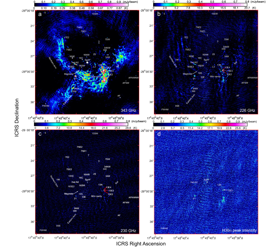
Figure 1: a Continuum map using Briggs weight at 343 GHz around Sgr A^∗ in the ALMA Cy.3 program (2015.1.01080.S.)(see Tsuboi et al. (2017b)). The angular resolution is $0\farcs 107\times 0\farcs 101,PA=-78^{\circ}$ in FWHM, which is shown as an oval at the lower left corner. This is a finding chart of the objects around Sgr A^∗. The position of of Sgr A^∗ was $\alpha_{\rm ICRS}$ = $17^{\rm h}45^{\rm m}40^{\rm s}.033903\pm 0^{\rm s}.0000034$,$\delta_{\rm ICRS}$= $-29^{\circ}00^{\prime}28\farcs 224140\pm 0\farcs 000506$ at $t_{\mathrm{obs}}=2016.693$ year using 2-D Gaussian fitting. The peak flux density of Sgr A^∗ at 343 GHz is derived to be $S_{\nu}{\mathrm{(343)}}=2182\pm 27$ mJy beam^-1. b Continuum map using natural weight at 226 GHz around Sgr A^∗ in the ALMA Cy.5 program (2017.1.00503.S.) (also see Tsuboi et al. (2019a)). The angular resolution is $0\farcs 037\times 0\farcs 025,PA=-86^{\circ}$ in FWHM, which is shown as an oval at the lower left corner. The position of Sgr A^∗ was $\alpha_{\rm ICRS}$ = $17^{\rm h}45^{\rm m}40^{\rm s}.40.03338820\pm 0^{\rm s}.00000025$, $\delta_{\rm ICRS}$= $-29^{\circ}00^{\prime}28\farcs 23047008\pm 0\farcs 00000147$ at $t_{\mathrm{obs}}=2017.773$ year (see text). The peak flux density of Sgr A^∗ at 226 GHz is derived to be $S_{\nu}{\mathrm{(226)}}=3069\pm 0.7$ mJy beam^-1. c Continuum map using natural weight at 230 GHz around Sgr A^∗ in the ALMA Cy.6 program (2017.1.00503.S.) The angular resolution is $\theta_{\mathrm{maj}}\times\theta_{\mathrm{min}}=0\farcs 027\times 0\farcs 024,PA=72^{\circ}$ in FWHM, which is shown as an oval at the lower left corner. The position of Sgr A^∗ was $\alpha_{\rm ICRS}$ = $17^{\rm h}45^{\rm m}40^{\rm s}.0329918\pm 0^{\rm s}.0000002$, $\delta_{\rm ICRS}$= $-29^{\circ}00^{\prime}28\farcs 242434\pm 0\farcs 000002$ at $t_{\mathrm{obs}}=2019.471$ year. The peak flux density of Sgr A^∗ at 230 GHz is derived to be $S_{\nu}{\mathrm{(226)}}=3569.8\pm 0.7$ mJy beam^-1 at $t_{\mathrm{obs}}=2019.471$. d Peak intensity map using natural weight around Sgr A^∗ in the H$30\alpha$ recombination line in the ALMA Cy.5 program (2017.1.00503.S.). The angular resolution is $0\farcs 035\times 0\farcs 023,PA=86^{\circ}$ in FWHM, which is shown as an oval at the lower left corner. The cross shows the position of Sgr A^∗.

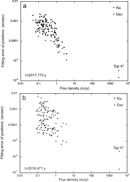
Figure 2: Relation between the flux density of the detected source and the 2-D Gaussian fitting positional error. a in the epoch of 2017.773 year. b in the epoch of 2019.471 year.

Figure 3: a Angular offsets between the star positions derived using Briggs and natural weights in the epochs of 2017.773 year. b Relation between the flux densities derived using Briggs and natural weights in the epoch of 2017.773 year.

3 Results

3.1 Continuum Maps and Positions of the Detected Objects

Figure 1a shows the continuum map using Briggs weight of the region within 0.4 pc of Sgr A^∗ at 343 GHz obtained in the ALMA Cy.3 program (2015.1.01080.S.)(Tsuboi et al. (2017b)). The observation epoch is $t_{\mathrm{Cy.3}}=2016.693$ y. The angular resolution is $0\farcs 107\times 0\farcs 101,PA=-78^{\circ}$ in FWHM. Although Sgr A^∗ is prominent in the figure, the GCMS which is composed of the Northern Arm(NA), Eastern Arm(EA) and Bar are also identified clearly. Therefore this figure is a finding chart of the objects around Sgr A^∗, which will be discussed.

Figures 1b shows the continuum map using natural weight at 226 GHz around Sgr A^∗ in the ALMA Cy.5 program (2017.1.00503.S.) (also see Tsuboi et al. (2019a)). The angular resolution is $0\farcs 037\times 0\farcs 025,PA=-86^{\circ}$ in FWHM. Sgr A^∗ is dominant in the figure, while the GCMS is identified vaguely. The position of Sgr A^∗ at 226 GHz was $\alpha_{\rm ICRS}$ = $17^{\rm h}45^{\rm m}40^{\rm s}.40.03338820\pm 0^{\rm s}.00000025$, $\delta_{\rm ICRS}$= $-29^{\circ}00^{\prime}28\farcs 23047008\pm 0\farcs 00000147$ at $t_{\mathrm{obs}}=2017.773$ year using 2-D Gaussian fitting for the continuum map using Briggs weight (CASA task, imfit). Although the positions of Sgr A^∗ using Briggs and natural weights are identical within the accuracy of $<1~{}\mu$as, we used the star positions with Briggs weight for the data of 2017.773 year in the following analysis because of the reason shown later. These positional errors include only fitting errors not calibration errors. In the case of Sgr A^∗, the signal-to-noise ratio ($SNR$) is equal to the dynamic range mentioned in S2.1, $SNR\gtrsim 2\times 10^{5}$. The very high $SNR$ is thought to make the very high nominal accuracy (Cf. Figure 2a). The peak flux density of Sgr A^∗ at 226 GHz is derived to be $S_{\nu}{\mathrm{(226)}}=3069\pm 0.7$ mJy beam^-1 at $t_{\mathrm{obs}}=2017.773$ year using 2-D Gaussian fitting. The absolute accuracy of the flux density should be as large as $10~{}\%$ based on the ALMA User Guide. The second prominent component in these figures is the IRS13E cluster which is centered around $\alpha_{\mathrm{ICRS}}\sim 17^{\mathrm{h}}45^{\mathrm{m}}39.^{\mathrm{s}}8,\delta_{\mathrm{ICRS}}\sim-29^{\circ}00^{\prime}29.\arcsec 8$. The IRS13E cluster has a very complicated structure extending to the south. The southern extension has been identified as the ionized gas flowing in the IRS13E cluster (Tsuboi et al. (2017b)). Other well-known IR objects around Sgr A^∗ including, the IRS16 cluster and IRS21 and so on are also clearly detected both in the continuum map (also see Figure 1a). They are labeled in the figures. The positions and flux densities of these objects are derived by 2-D Gaussian fitting to the continuum map and summarized in Table 2. The angular extent of these objects is also estimated by 2-D Gaussian deconvolution. When the estimated extent is smaller than the beam size, the object is determined to be point-like. The total number of the detected objects around Sgr A^∗ is 65. The detected objects are distributed in the angular distance from Sgr A^∗ from $\sim 1\arcsec$ to $\sim 13\arcsec$. The flux densities of the detected objects are distributed in the range from $\sim 0.05$ mJy to $\sim 4$ mJy. Additionally, the positions, flux densities, and angular extent of these objects at 343 GHz are derived by the same procedure. They are also summarized in Table 2.

Figures 1c shows the continuum map using natural weight at at 230 GHz around Sgr A^∗ in the ALMA Cy.6 program (2018.1.001124.S.). The angular resolution is $0\farcs 027\times 0\farcs 024,PA=72^{\circ}$ in FWHM. The position of Sgr A^∗ was $\alpha_{\rm ICRS}$ = $17^{\rm h}45^{\rm m}40^{\rm s}.03299175\pm 0^{\rm s}.00000017$, $\delta_{\rm ICRS}$= $-29^{\circ}00^{\prime}28\farcs 24243361\pm 0\farcs 00000180$ at $t_{\mathrm{obs}}=2019.471$ year using 2-D Gaussian fitting. The peak flux density of Sgr A^∗ at 230 GHz is derived to be $S_{\nu}\mathrm{(226)}=3569.8\pm 0.7$ mJy beam^-1 at $t_{\mathrm{obs}}=2019.471$ using 2-D Gaussian fitting. The positions and flux densities of the objects around Sgr A^∗ are also derived by 2D Gaussian fitting and summarized in Table 2. All the objects detected in the Cy.5 observation are detected except one object, No.64, which would be under the detection limit around the edge of the FOV.

As mentioned above, the positions of the detected objects are derived by 2-D Gaussian fitting to the continuum maps. We checked the relation between the flux density and the fitting positional error. Figures 2a and 2b show the relations observed at 2017.773 and 2019.471 years, respectively. The fitting positional error seems to decrease with increasing the flux density both in the epochs. This is thought to be caused by that the fitting is affected by signal-to-noise ratio of the object. In the epochs of 2017.773 year, the fitting positional error is similar both in right ascension and declination and up to a few mas (see Figure 2a). On the other hand, the error in the epochs of 2019.471 year is fairly different in the right ascension and declination (see Figure 2b). Although the error in right ascension is almost less than 1 mas, the error in declination often reaches to several mas. This situation may be caused especially by the artifact around Sgr A^∗ mentioned above in the observation data at 2019.471 year. If the positional error of 1 mas is in these observations, this causes the ambiguity of $\sim 30$ km s^-1 as proper motion.

Figure 3a shows the angular offsets between the positions relative to Sgr A^∗ derived using Briggs and natural weights in the epochs of 2017.773 year. The error bars in the figure indicate the fitting errors. Because the synthesized beam size (beam solid angle) using natural weight, is $60\%$ larger than that using Briggs weight, the former is easily affected by the extended emission around the object. Especially, if the extended emission is not uniform, the position derived by 2-D Gaussian fitting should be shifted from the original position. Although the angular offsets of almost stars are less than $<2$ mas, several stars have relatively large offset up to 5 mas. The stars with large offset have large fitting errors. Because these stars are, for the most part, located in the IRS13E and IRS13N clusters, the large offsets would be caused by complex extended emission around stars in the clusters (see Figure 9). Therefore, it is better to use the star positions with Briggs weight for the data of 2017.773 year. On the other hand, we used unavoidably the star positions with natural weight for the data of 2019.471 year because the stars with weak intensity are undetectable because of the insufficient $SNR$ if we use Briggs weight. However, because the beam with natural weight for the data of 2019.471 year, $0\farcs 027\times 0\farcs 024$, is comparable with the beam with Briggs weight for the data of 2017.773 year, $0\farcs 029\times 0\farcs 020$, this would not significantly affect the derivation of proper motions. In addition, Figure 3b shows the relation between the flux densities derived using Briggs and natural weights in the epochs of 2017.773 year. As mentioned above, if the beam solid angle is larger the measurement is more easily affected by the extended emission. There is a trend that the flux densities derived using natural weight are somewhat larger than those derived using Briggs weight. Especially, this trend is noticeable in the flux density less than 1 mJy. The trend may be caused by that larger beam solid angle samples larger extended emission. This is another reason for that we used Briggs weight whenever possible.

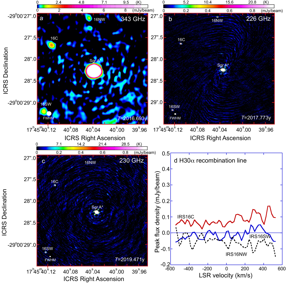
Figure 4: a Enlarged continuum map using uniform weight in the vicinity within 0.1 pc of Sgr A^∗ at 343 GHz. The angular resolution is $0\farcs 102\times 0\farcs 096,PA=80^{\circ}$ in FWHM, which is shown as an oval at the lower left corner. The position of Sgr A^∗ at 343 GHz is $\alpha_{\rm ICRS}$ = $17^{\rm h}45^{\rm m}40^{\rm s}.033903\pm 0^{\rm s}.000034$, $\delta_{\rm ICRS}$= $-29^{\circ}00^{\prime}28\farcs 224140\pm 0\farcs 000506$ at 2016.693 year. The peak flux density of Sgr A^∗ is $2182\pm 27$ mJy beam^-1 at 343 GHz. b Enlarged continuum map using Briggs weight in the same area at 226 GHz. The angular resolution is $0\farcs 029\times 0\farcs 020,PA=86^{\circ}$ in FWHM, which is shown as an oval at the lower left corner. The position of Sgr A^∗ at 226 GHz is $\alpha_{\rm ICRS}$ = $17^{\rm h}45^{\rm m}40^{\rm s}.03338820\pm 0^{\rm s}.00000025$, $\delta_{\rm ICRS}$= $-29^{\circ}00^{\prime}28\farcs 23047001\pm 0\farcs 0000015$ at 2017.773 year. The peak flux density of Sgr A^∗ is $S_{\nu}=3069\pm 0.7$ mJy beam^-1 at 226 GHz (also see Tsuboi et al. (2017a), 2019). c Enlarged continuum map using natural weight in the same area at 230 GHz . The angular resolution is $0\farcs 027\times 0\farcs 025,PA=72^{\circ}$ in FWHM, which is shown as an oval at the lower left corner. The position of Sgr A^∗ at 230 GHz is $\alpha_{\rm ICRS}$ = $17^{\rm h}45^{\rm m}40^{\rm s}.03299175\pm 0^{\rm s}.00000017$, $\delta_{\rm ICRS}$= $-29^{\circ}00^{\prime}28\farcs 2424336\pm 0\farcs 0.0000018$ at 2019.471 year. The peak flux density of Sgr A^∗ is $S_{\nu}=3570\pm 0.7$ mJy beam^-1 at 230 GHz (also see Tsuboi et al. (2017a), 2019). d Line profiles of IRS16NW, 16C and 16SW in H30$\alpha$ recombination line, which were obtained in the ALMA Cy.5 program.

3.2 Region within 0.1 pc of Sgr A^∗

Figures 4a, 4b, and 4c show the enlarged continuum maps in the vicinity within 0.1 pc of Sgr A^∗ at 343, 226 and 230 GHz, respectively. Three famous WR stars, IRS16NW, IRS16C, and IRS16SW, are detected clearly around Sgr A^∗ although Sgr A^∗ is dominant in these figures. In Figures 4b, and 4c, the extended component larger than the beam size is not detected around Sgr A^∗ at these frequencies, or Sgr A^∗ is detected as a point source. Accordingly, the physical extent of the emitting region of Sgr A^∗ is thought to be much less than that of the beam size, $25~{}\mathrm{mas}\sim 0\farcs 001$ pc. Similarly, the extended components larger than the beam size are not detected around IRS16NW, IRS16C, and IRS16SW.

There are some faint patches, $S_{\nu}\sim 0.2$ mJy beam^-1, in the immediate vicinity ($\lesssim 0\farcs 25\sim 0.01$ pc) of Sgr A^∗ in Figures 4b and 4c. These patches are probably residuals of the side lobes after applying the “self-calibration” method. If the patches are residuals of the side lobes, the dynamic range of the map is proved to reach to $\gtrsim 100000$ immediately around Sgr A^∗. Although famous S stars are located in this area, the patches are probably not these stars because the distribution resembles to that of the side lobe not that of the stars. It is considered that the S stars are too faint to be detected in these observations because they have the spectral type of B.

The peak flux densities of Sgr A^∗ are $S_{\nu}=2.182\pm 0.027$ Jy beam^-1 at 343 GHz at 2016.693 year, $S_{\nu}=3.069\pm 0.0007$ Jy beam^-1 at 226 GHz at 2017.773 year, and $S_{\nu}=3.570\pm 0.0007$ Jy beam^-1 at 230 GHz at 2019.471 year, respectively. The flux density of Sgr A^∗ is variable temporally in the millimeter and sub-millimeter wavelengths as well known (e.g. Miyazaki, Tsutsumi & Tsuboi (2004)). Therefore, the spectral index cannot be derived using these data.

3.3 H$30\alpha$ Recombination Line Map

Figures 1d shows the peak intensity map in the H$30\alpha$ recombination line obtained in the Cy.5 observation. The cross in the figure shows the position of Sgr A^⋆. The widely extended structures of the GCMS are almost disappeared in Figures 1c. However, IRS13E3 and the southern extension are still prominent. IRS21, HeI-N2, and IRS13N cluster are also identified although they are faint. The disappearance of the GCMS is considered to be caused by that the structure is mainly consist of extended components over the maximum detectable angular scale of the Cy.5 observation and they are resolved-out. Many IR stars around Sgr A^∗ including IRS16NW, IRS16C, IRS16SW, and so on are thought to be WR stars, which should have ionized gas outflows. The radial velocity derived from the H$30\alpha$ recombination line data is useful to obtain the 3-D kinematics. However, such ionized gas outflows were not detected in the H$30\alpha$ recombination line data of the Cy.5 observation. Figure 4d shows the line profiles of IRS16NW, IRS16C, and IRS16SW in the H$30\alpha$ recombination line as examples of the non-detection.

3.4 Flux densities of Member Stars of the Nuclear Star Cluster

We checked the reproducibility in the observed flux densities. Figure 5 shows the relation between the flux densities at 226 and 230 GHz, which have been observed at 2017.773 and 2019.471 year, respectively. The detected objects are mostly WR stars. The centimeter-wave observations of WR stars in the Galactic disk have been performed using VLA and ATCA (e.g. Cappa et al. (2004), Andrews et al. (2019)). Although the intensity variabilities of some WR stars have been reported (e.g. Cappa et al. (2004)), it is an open question whether WR stars are usually variable in the timescale of less than several years or not. We assumed here that WR stars are not variable significantly within the elapse time. Although the flux densities at 2019.471 year are nearly equal to or slightly smaller than those at 2017.773 year in the intensity region of $S_{\nu}\gtrsim 1.5$ mJy, the former are somewhat smaller than the latter in the weaker intensity region. Moreover, the data points are scattered randomly in the intensity region of $S_{\nu}\lesssim 0.4$ mJy. The dependence on the intensity would indicate that the difference is caused by the reproducibility rather than time variation of the objects. The degree of differences between observed flux densities would indicate the degree of reproducibility in the observed flux densities. In addition, the random behavior in the intensity region of $S_{\nu}\lesssim 0.4$ mJy may be also caused by the artifact mentioned previously in the observation data at 2019.471 year .

There is a remaining issue what is the spectrum in mm-submm wavelengths of detected objects. This issue affects the capability of astrometry with ALMA. If many objects have spectra dominated by dusts or the spectral index is steeper than $\alpha\gtrsim 2$ ($S_{\nu}\propto\nu^{\alpha}$), shorter wavelength observations should detect many fainter objects ($S_{\nu}(343)\gtrsim 2\times S_{\nu}(230)$). On the other hand, if many objects have spectra dominated by ionized gas or the spectral index is as flat as $\alpha\sim-0.1$, longer wavelength observations should be promising in order to detect many fainter objects ($FOV\sim 60\arcsec$ at 90 GHz). Although the spectrum indexes of WR stars in centimeter-wavelength are known to be widely scattered (Andrews et al. (2019)), those in mm-submm wavelengths are not yet studied comprehensively. The WR stars in the NSC may be good observation targets to solve the issue because they are located at the same distance from us. Figure 6 shows the comparison between flux densities of detected objects at 230 and 343 GHz. The flux densities at 230 GHz are the means of those at 226 and 230 GHz which are summarized in Table 1. The linear lines indicate the spectral indexes of $S_{\nu}\propto\nu^{-0.1}$, $S_{\nu}\propto\nu^{1}$ and $S_{\nu}\propto\nu^{2}$, respectively. Spectral indexes of the detected WR stars are scattered apparently in the wide range from $\alpha\sim-0.1$ to $\alpha\sim 2$. However, it is impossible to determine if this is due to that they have such scattered intrinsic spectral indexes or the flux densities are variable in the observation duration ($\sim 2.8$ years). Therefore it is inconclusive (from the data) whether shorter or longer wavelength observations are advantageous over one another.

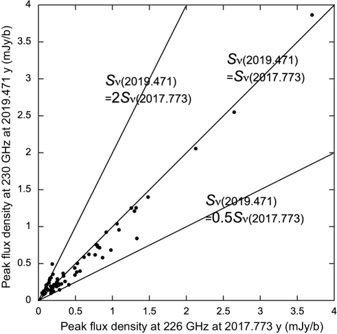
Figure 5: Relation between the flux densities at 226 and 230 GHz, which have been observed at 2017.773 and 2019.471 year, respectively. Linear lines indicate the relations of $S_{\nu}(2019.471)=2S_{\nu}(2017.773)$, $S_{\nu}(2019.471)=S_{\nu}(2017.773)$ and $S_{\nu}(2019.471)=0.5S_{\nu}(2017.773)$, respectively.

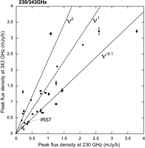
Figure 6: Comparison between flux densities of detected objects at 230 and 343 GHz. The flux densities at 230 GHz are the means of those at 226 and 230 GHz which are summarized in Table 2. Linear lines indicate the spectra with $S_{\nu}\propto\nu^{-0.1}$, $S_{\nu}\propto\nu^{1}$ and $S_{\nu}\propto\nu^{2}$, respectively.

Table 2: Positions, Flux Densities and Angular Extents of the Detected Objects around Sagittarius A^∗

No.	Name	$\alpha_{\mathrm{Cy.3}}-17^{\rm h}45^{\rm m~{}1}$	$\alpha_{\mathrm{Cy.5}}-17^{\rm h}45^{\rm m~{}2}$	$\alpha_{\mathrm{Cy.6}}-17^{\rm h}45^{\rm m~{}3}$	$-\delta_{\mathrm{Cy.3}}+29^{\circ}00^{\prime~{}1}$	$-\delta_{\mathrm{Cy.5}}+29^{\circ}00^{\prime~{}2}$	$-\delta_{\mathrm{Cy.6}}+29^{\circ}00^{\prime~{}3}$
		[s]	[s]	[s]	[$\arcsec$]	[$\arcsec$]	[$\arcsec$]
1	Sgr A∗	40.033903$\pm$0.000034	40.03338820$\pm$0.00000025	40.03299175$\pm$0.00000017	28.224140$\pm$0.000506	28.23047008$\pm$0.0000015	28.24243361$\pm$0.0000018
2	IRS16C	40.10919$\pm$0.00016	40.10779$\pm$0.00001	40.10623$\pm$0.00005	27.62910$\pm$0.00205	27.62384$\pm$0.00003	27.62363$\pm$0.00043
3	IRS16NW	40.04378$\pm$0.00028	40.04312$\pm$0.00001	40.04354$\pm$0.00005	27.00140$\pm$0.00434	27.00745$\pm$0.00007	27.01943$\pm$0.00056
4	IRS16SW	40.12218$\pm$0.00008	40.12243$\pm$0.00001	40.12275$\pm$0.00004	29.15942$\pm$0.00113	29.15940$\pm$0.00005	29.16482$\pm$0.00047
5	IRS29	39.91689$\pm$0.00030	39.91802$\pm$0.00003	39.91802$\pm$0.00007	26.86776$\pm$0.00362	26.90544$\pm$0.00104	26.92769$\pm$0.00062
6	IRS16CC	-	40.18365$\pm$0.00005	40.18278$\pm$0.00018	-	27.58607$\pm$0.00032	27.59042$\pm$0.00137
7	IRS16SE1	-	40.18123$\pm$0.00004	40.18208$\pm$0.00018	-	29.31932$\pm$0.00026	29.31145$\pm$0.00255
8	IRS16S	-	40.14119$\pm$0.00004	40.14220$\pm$0.00007	-	30.11295$\pm$0.00024	30.12517$\pm$0.0009
9	Magnetar	40.16418$\pm$0.00006	40.16359$\pm$0.00001	40.16335$\pm$0.00007	29.89075$\pm$0.00069	29.88759$\pm$0.00007	29.88852$\pm$0.00088
10	IRS13N$\alpha$U	-	39.83333$\pm$0.00009	39.83429$\pm$0.00020	-	29.54574$\pm$0.00115	29.54607$\pm$0.00303
11	IRS13N$\alpha$L	-	39.83231$\pm$0.00009	39.83123$\pm$0.00006	-	29.65141$\pm$0.00028	29.65500$\pm$0.00039
12	IRS13N$\delta$	-	39.81219$\pm$0.00013	39.81167$\pm$0.00040	-	28.99155$\pm$0.00087	28.99629$\pm$0.00304
13	IRS13N$\epsilon$	-	39.81175$\pm$0.00005	39.81186$\pm$0.00047	-	29.15795$\pm$0.00032	29.15393$\pm$0.00697
14	IRS16NE	40.25621$\pm$0.00005	40.25585$\pm$0.00001	40.25583$\pm$0.00001	27.33097$\pm$0.00058	27.34910$\pm$0.00001	27.37654$\pm$0.00010
15	IRS33SW	-	40.01189$\pm$0.00007	40.01039$\pm$0.00015	-	31.30012$\pm$0.00034	31.30508$\pm$0.00047
16	IRS16SE2	40.26062$\pm$0.00010	40.26065$\pm$0.00001	40.26061$\pm$0.00003	29.35163$\pm$0.00134	29.34682$\pm$0.00005	29.35070$\pm$0.00032
17	IRS33E	40.09114$\pm$0.00008	40.09116$\pm$0.00003	40.09169$\pm$0.00006	31.37651$\pm$0.00145	31.37890$\pm$0.00021	31.39145$\pm$0.00109
18	IRS13Ef	-	39.82013$\pm$0.00002	39.81910$\pm$0.00007	-	29.90060$\pm$0.00038	29.90373$\pm$0.00203
19	IRS13N$\gamma$	-	39.79274$\pm$0.00008	39.79232$\pm$0.00021	-	29.12088$\pm$0.00087	29.12138$\pm$0.00310
20	IRS13E6	-	39.79663$\pm$0.00017	39.79456$\pm$0.00007	-	29.70879$\pm$0.00092	29.72235$\pm$0.00189
21	IRS13E1	-	39.80485$\pm$0.00006	39.80268$\pm$0.00009	-	29.93819$\pm$0.00042	29.92984$\pm$0.00082
22	IRS13Ea	-	39.78680$\pm$0.00009	39.78515$\pm$0.00022	-	29.65390$\pm$0.00070	29.67294$\pm$0.00235
23	IRS13Eb	-	39.78750$\pm$0.00005	39.78676$\pm$0.00009	-	29.71359$\pm$0.00052	29.72144$\pm$0.00154
24	IRS13E3	39.78884$\pm$0.00003	39.78929$\pm$0.00007	39.78863$\pm$0.00007	29.76710$\pm$0.00047	29.75799$\pm$0.00029	29.76952$\pm$0.00049
25	IRS13E4	39.78455$\pm$0.00002	39.78294$\pm$0.00003	39.78163$\pm$0.00007	29.64059$\pm$0.00024	29.63148$\pm$0.00018	29.64326$\pm$0.00061
26	IRS13Ec	-	39.78738$\pm$0.00002	39.78656$\pm$0.00006	-	29.78667$\pm$0.00010	29.80080$\pm$0.00051
27	IRS21-LR	-	40.20498$\pm$0.00016	40.20405$\pm$0.00024	-	31.03001$\pm$0.00137	31.04889$\pm$0.00230
28	-	-	39.78932$\pm$0.00007	39.78926$\pm$0.00005	-	29.87323$\pm$0.00045	29.88445$\pm$0.00045
29	IRS13Ed	-	39.78608$\pm$0.00015	39.78545$\pm$0.00005	-	29.85531$\pm$0.00167	29.87340$\pm$0.00117
30	IRS13E2	39.78666$\pm$0.00001	39.78542$\pm$0.00001	39.78415$\pm$0.00001	29.93966$\pm$0.00009	29.95779$\pm$0.00009	29.96853$\pm$0.00007
31	IRS13E5	-	39.77233$\pm$0.00005	39.77133$\pm$0.00011	-	29.67291$\pm$0.00072	29.68135$\pm$0.00246
32	-	-	39.76755$\pm$0.00005	39.76611$\pm$0.00003	-	29.75879$\pm$0.00058	29.76175$\pm$0.00005
33	IRS13Ee	-	39.78124$\pm$0.00007	39.78060$\pm$0.00010	-	30.14124$\pm$0.00064	30.14738$\pm$0.00144
34	-	-	39.75869$\pm$0.00004	39.75748$\pm$0.00007	-	29.92265$\pm$0.00023	29.92835$\pm$0.00049

¹ The observation epoch is $t_{\mathrm{Cy.3}}=2016.693$ y, ² The observation epoch is $t_{\mathrm{Cy.5}}=2017.773$ y. ³ The observation epoch is $t_{\mathrm{Cy.6}}=2019.471$ y. ⁴ When the deconvolved image size is much smaller than the synthesized beam ($30$ mas at 230 GHz, $40$ mas at 226 GHz and $100$ mas at 343 GHz), we define that it is a point source, P. ⁵ The peak flux density is derived by 2D Gaussian fit.

Table 2: Continued.

No.	Name	$\alpha_{\mathrm{Cy.3}}-17^{\rm h}45^{\rm m~{}1}$	$\alpha_{\mathrm{Cy.5}}-17^{\rm h}45^{\rm m~{}2}$	$\alpha_{\mathrm{Cy.6}}-17^{\rm h}45^{\rm m~{}3}$	$-\delta_{\mathrm{Cy.3}}+29^{\circ}00^{\prime~{}1}$	$-\delta_{\mathrm{Cy.5}}+29^{\circ}00^{\prime~{}2}$	$-\delta_{\mathrm{Cy.6}}+29^{\circ}00^{\prime~{}3}$
		[s]	[s]	[s]	[$\arcsec$]	[$\arcsec$]	[$\arcsec$]
35	-	-	39.78882$\pm$0.00007	39.78793$\pm$0.00002	-	30.63723$\pm$0.00065	30.64490$\pm$0.00044
36	-	-	39.76084$\pm$0.00015	39.75933$\pm$0.00003	-	25.99978$\pm$0.00111	25.99888$\pm$0.00049
37	IRS34W	39.72258$\pm$0.00001	39.72198$\pm$0.00001	39.72130$\pm$0.00002	26.71637$\pm$0.00013	26.72453$\pm$0.00005	26.74586$\pm$0.00021
38	IRS3	39.85890$\pm$0.00022	39.85866$\pm$0.00007	39.85885$\pm$0.00003	24.42073$\pm$0.00296	24.41246$\pm$0.00027	24.42189$\pm$0.00023
39	IRS7SE2	-	40.26501$\pm$0.00006	40.26533$\pm$0.00013	-	24.76677$\pm$0.00041	24.77751$\pm$0.00187
40	IRS13W	39.69455$\pm 0.00001$	39.69530$\pm$0.00005	39.69425$\pm$0.00003	29.82434$\pm 0.00025$	29.85065$\pm$0.00031	29.86040$\pm$0.00035
41	IRS34NW	39.742516$\pm$0.00006	39.74234$\pm$0.00004	39.74091$\pm$0.00011	25.45558$\pm 0.00138$	25.43943$\pm$0.00032	25.45611$\pm$0.00090
42	-	39.718828$\pm$0.00001	39.72013$\pm$0.00014	39.71996$\pm$0.00008	31.04740$\pm 0.00025$	31.05306$\pm$0.00065	31.05975$\pm$0.00087
43	-	-	39.76859$\pm$0.00008	39.76793$\pm$0.00003	-	32.05287$\pm$0.00115	32.04728$\pm$0.00058
44	IRS6E	-	39.64166$\pm$0.00003	39.64096$\pm$0.00019	-	27.37381$\pm$0.00028	27.37978$\pm$0.00342
45	IRS7	40.03641$\pm$0.00003	40.03569$\pm$0.00004	40.03572$\pm$0.00009	22.73652$\pm$0.00098	22.76113$\pm$0.00020	22.78018$\pm$0.00132
46	IRS7NE1	40.09975$\pm$0.00005	40.09938$\pm$0.00002	40.09862$\pm$0.00003	22.38461$\pm$0.00058	22.38118$\pm$0.00011	22.38746$\pm$0.00030
47	IRS7SW	39.73254$\pm$0.00004	39.73235$\pm$0.00004	39.73176$\pm$0.00007	23.33843$\pm$0.00080	23.35198$\pm$0.00017	23.36886$\pm$0.00096
48	IRS9NW	40.25797$\pm 0.00001$	40.25736$\pm$0.00002	40.25786$\pm$0.00005	33.78795$\pm 0.00007$	33.79589$\pm$0.00012	33.80294$\pm$0.00053
49	IRS7W	39.85270$\pm$0.00005	39.85306$\pm$0.00010	39.85308$\pm$0.00024	22.24258$\pm$0.00050	22.23176$\pm$0.00118	22.24105$\pm$0.00239
50	IRS9W	40.26824$\pm$0.00024	40.26429$\pm$0.00014	40.26421$\pm$0.00013	33.95782$\pm$0.00219	33.93974$\pm$0.00183	33.94384$\pm$0.00144
51	IRS7E2	40.37711$\pm$0.00008	40.37628$\pm$0.00002	40.37660$\pm$0.00004	23.27175$\pm$0.00110	23.27927$\pm$0.00009	23.29230$\pm$0.00037
52	IRS7NE2	40.15053$\pm$0.00002	40.14897$\pm$0.00004	40.14792$\pm$0.00012	21.68862$\pm$0.00033	21.69063$\pm$0.00021	21.69902$\pm$0.00108
53	IRS6W	-	39.44574$\pm$0.00007	39.44569$\pm$0.00006	-	26.76967$\pm$0.00038	26.76884$\pm$0.00043
54	IRS6NW	-	39.445294$\pm$0.00007	39.44469$\pm$0.00003	-	26.51045$\pm$0.00032	26.52010$\pm$0.00041
55	AFNW	39.45235$\pm$0.00005	39.45158$\pm$0.00001	39.45100$\pm$0.00002	31.84201$\pm$0.00064	31.85837$\pm$0.00003	31.87609$\pm$0.00023
56	-	-	40.03150$\pm$0.00006	40.03133$\pm$0.00010	-	19.64663$\pm$0.00040	19.65594$\pm$0.00163
57	IRS10E	-	40.61884$\pm$0.00007	40.61920$\pm$0.00006	-	24.05270$\pm$0.00032	24.07079$\pm$0.00062
58	-	-	40.75190$\pm$0.00003	40.75113$\pm$0.00005	-	27.98623$\pm$0.00020	28.00458$\pm$0.00069
59	AF	39.53955$\pm$0.00002	39.53929$\pm$0.00001	39.53925$\pm$0.00001	35.11251$\pm$0.00032	35.11620$\pm$0.00002	35.12552$\pm$0.00011
60	AFNWNW	39.30302$\pm$0.00001	39.30261$\pm$0.00003	39.30239$\pm$0.00003	30.79032$\pm$0.00012	30.79656$\pm$0.00016	30.81048$\pm$0.00033
61	IRS9SE	-	40.46340$\pm$0.00002	40.46280$\pm$0.00006	-	36.43745$\pm$0.00021	36.45220$\pm$0.00056
62	-	-	39.37495$\pm$0.00009	39.37430$\pm$0.00005	-	33.49673$\pm$0.00056	33.50216$\pm$0.00044
63	IRS15SW	-	39.91264$\pm$0.00008	39.91200$\pm$0.00002	-	18.21589$\pm$0.00044	18.23050$\pm$0.00021
64	-	-	39.35564$\pm$0.00003	-	-	33.95517$\pm$0.00018	-
65	-	-	40.13729$\pm$0.00001	40.13680$\pm$0.00001	-	16.52472$\pm$0.00006	16.53267$\pm$0.00011
66	IRS5	-	40.69051$\pm$0.00012	40.69057$\pm$0.00024	-	18.43462$\pm$0.00075	18.45965$\pm$0.00375

¹ The observation epoch is $t_{\mathrm{Cy.3}}=2016.693$ y, ² The observation epoch is $t_{\mathrm{Cy.5}}=2017.773$ y. ³ The observation epoch is $t_{\mathrm{Cy.6}}=2019.471$ y. ⁴ When the deconvolved image size is much smaller than the synthesized beam ($30$ mas at 230 GHz, $40$ mas at 226 GHz and $100$ mas at 343 GHz), we define that it is a point source, P. ⁵ The peak flux density is derived by 2D Gaussian fit.

Table 2: Continued.

No.	SizeCy.3, $PA^{~{}1,4}$	SizeCy.5, $PA^{~{}2,4}$	SizeCy.6, $PA^{~{}3,4}$	$S_{\nu}(343)^{1,5}$	$S_{\nu}(226)^{2,5}$	$S_{\nu}(230)^{3,5}$
	[mas$\times$mas, deg.]	[mas$\times$mas, deg.]	[mas$\times$mas, deg.]	[mJy beam-1]	[mJy beam-1]	[mJy beam-1]
1	P	P	P	2182$\pm$27	3069$\pm$0.7	3570$\pm$0.7
2	P	P	P	1.358$\pm$0.053	1.483$\pm$0.006	1.400$\pm$0.065
3	P	P	P	0.724$\pm$0.049	0.828$\pm$0.008	0.710$\pm$0.040
4	P	P	P	0.938$\pm$0.022	1.298$\pm$0.010	1.209$\pm$0.056
5	P	P	P	0.307$\pm$0.022	0.335$\pm$0.009	0.366$\pm$0.022
6	-	P	P	-	0.196$\pm$0.009	0.178$\pm$0.028
7	-	P	P	-	0.182$\pm$0.004	0.215$\pm$0.022
8	-	P	P	-	0.175$\pm$0.005	0.157$\pm$0.016
9	P	P	P	3.141$\pm$0.044	1.331$\pm$0.013	0.840$\pm$0.064
10	-	$56\times 27,~{}161$	$50\times 10,~{}142$	-	0.132$\pm$0.011	0.142$\pm$0.019
11	-	P	P	-	0.070$\pm$0.004	0.081$\pm$0.005
12	-	$116\times 23,~{}121$	$58\times 26,~{}112$	-	0.117$\pm$0.007	0.153$\pm$0.028
13	-	P	$57\times 25,~{}39$	-	0.092$\pm$0.004	0.103$\pm$0.027
14	P	P	P	3.219$\pm$0.040	3.700$\pm$0.006	3.865$\pm$0.037
15	-	$50\times 22,95$	$70\times 14,93$	-	0.109$\pm$0.004	0.156$\pm$0.008
16	P	P	P	1.248$\pm$0.032	1.089$\pm$0.007	0.955$\pm$0.034
17	P	P	P	0.660$\pm$0.015	0.981$\pm$0.025	0.683$\pm$0.056
18	-	$48\times 33,~{}172$	$48\times 17,~{}6$	-	0.361$\pm$0.006	0.258$\pm$0.020
19	-	P	$46\times 14,~{}141$	-	0.106$\pm$0.006	0.207$\pm$0.031
20	-	$49\times 19,~{}106$	P	-	0.121$\pm$0.004	0.153$\pm$0.015
21	-	P	P	-	0.142$\pm$0.007	0.241$\pm$0.011
22	-	P	P	-	0.284$\pm$0.019	0.144$\pm$0.022
23	-	$49\times 34,~{}131$	$36\times 26,~{}5$	-	0.519$\pm$0.014	0.384$\pm$0.032
24	P	P	$41\times 19,~{}100$	5.053$\pm$0.036	0.780$\pm$0.029	0.756$\pm$0.046
25	$96\times 33,~{}133$	P	P	1.345$\pm$0.007	0.803$\pm$0.022	0.727$\pm$0.046
26	-	$68\times 29,~{}90$	$38\times 26,~{}80$	-	0.766$\pm$0.006	0.618$\pm$0.022
27	-	48$\times$26, 119	44$\times$31, 111	-	0.255$\pm$0.022	0.291$\pm$0.040
28	-	52$\times$25, 112	P	-	0.340$\pm$0.011	0.331$\pm$0.014
29	-	$41\times 32,~{}106$	$32\times 11,~{}173$	-	0.494$\pm$0.027	0.346$\pm$0.021
30	P	P	P	2.790$\pm$0.005	2.127$\pm$0.013	2.057$\pm$0.014
31	-	P	$37\times 15,~{}11$	-	0.156$\pm$0.007	0.301$\pm$0.036
32	-	$49\times 41,~{}44$	P	-	0.412$\pm$0.012	0.213$\pm$0.009
33	-	P	P	-	0.249$\pm$0.013	0.249$\pm$0.023
34	-	P	P	-	0.170$\pm$0.004	0.098$\pm$0.006

¹ The observation epoch is $t_{\mathrm{Cy.3}}=2016.693$ y, ² The observation epoch is $t_{\mathrm{Cy.5}}=2017.773$ y. ³ The observation epoch is $t_{\mathrm{Cy.6}}=2019.471$ y. ⁴ When the deconvolved image size is much smaller than the synthesized beam ($30$ mas at 230 GHz, $40$ mas at 226 GHz and $100$ mas at 343 GHz), we define that it is a point source, P. ⁵ The peak flux density is derived by 2D Gaussian fit.

Table 2: Continued.

No.	SizeCy.3, $PA^{~{}1,4}$	SizeCy.5, $PA^{~{}2,4}$	SizeCy.6, $PA^{~{}3,4}$	$S_{\nu}(343)^{1,5}$	$S_{\nu}(226)^{2,5}$	$S_{\nu}(230)^{3,5}$
	[mas$\times$mas, deg.]	[mas$\times$mas, deg.]	[mas$\times$mas, deg.]	[mJy beam-1]	[mJy beam-1]	[mJy beam-1]
35	-	P	P	-	0.187$\pm$0.007	0.494$\pm$0.012
36	-	P	P	-	0.049$\pm$0.004	0.103$\pm$0.005
37	P	P	P	2.112$\pm$0.005	1.320$\pm$0.009	1.253$\pm$0.027
38	$126\times 92,~{}168$	P	P	0.714$\pm$0.031	0.277$\pm$0.013	0.207$\pm$0.007
39	-	P	P	-	0.105$\pm$0.007	0.177$\pm$0.022
40	P	P	P	0.178$\pm 0.001$	0.164$\pm$0.008	0.194$\pm$0.007
41	P	P	P	$0.423\pm 0.007$	0.186$\pm$0.008	0.158$\pm$0.011
42	$161\times 117$, 168	P	$35\times 19$, 131	1.316$\pm 0.039$	0.149$\pm$0.010	0.276$\pm$0.015
43	-	P	$64\times 36$, 158	-	0.171$\pm$0.011	0.309$\pm$0.006
44	-	P	$41\times 10$, 30	-	0.205$\pm$0.005	0.123$\pm$0.020
45	P	P	P	0.339$\pm$0.004	0.312$\pm$0.010	0.225$\pm$0.025
46	$173\times 137,~{}137$	P	P	1.058$\pm$0.014	0.493$\pm$0.007	0.440$\pm$0.014
47	P	P	P	0.619$\pm$0.010	0.526$\pm$0.014	0.503$\pm$0.040
48	P	P	P	1.287$\pm 0.002$	0.915$\pm$0.015	0.926$\pm$0.048
49	P	P	P	0.143$\pm$0.003	0.245$\pm$0.019	0.236$\pm$0.023
50	$236\times 153,~{}69$	P	$31\times 17,~{}52$	0.632$\pm$0.018	0.209$\pm$0.027	0.214$\pm$0.021
51	P	P	P	0.697$\pm$0.017	0.682$\pm$0.010	0.625$\pm$0.025
52	P	P	P	0.222$\pm$0.002	0.235$\pm$0.006	0.202$\pm$0.025
53	-	P	P	-	0.169$\pm$0.009	0.131$\pm$0.006
54	-	P	P	-	0.070$\pm$0.005	0.127$\pm$0.004
55	P	P	P	1.591$\pm$0.065	1.256$\pm$0.005	1.252$\pm$0.029
56	-	P	P	-	0.082$\pm$0.005	0.1180.012
57	-	P	P	-	0.089$\pm$0.004	0.096$\pm$0.005
58	-	P	P	-	0.246$\pm$0.006	0.190$\pm$0.011
59	P	P	P	3.217$\pm$0.109	2.647$\pm$0.009	2.549$\pm$0.030
60	P	P	P	1.263$\pm$0.003	0.794$\pm$0.018	0.749$\pm$0.025
61	-	P	P	-	0.564$\pm$0.014	0.398$\pm$0.026
62	-	P	P	-	0.265$\pm$0.018	0.234$\pm$0.012
63	-	P	P	-	0.616$\pm$0.038	0.586$\pm$0.013
64	-	P	-	-	0.096$\pm$0.003	-
65	-	P	P	-	1.063$\pm$0.009	1.039$\pm$0.012
66	-	P	P	-	0.196$\pm$0.011	0.356$\pm$0.017

¹ The observation epoch is $t_{\mathrm{Cy.3}}=2016.693$ y, ² The observation epoch is $t_{\mathrm{Cy.5}}=2017.773$ y. ³ The observation epoch is $t_{\mathrm{Cy.6}}=2019.471$ y. ⁴ When the deconvolved image size is much smaller than the synthesized beam ($30$ mas at 230 GHz, $40$ mas at 226 GHz and $100$ mas at 343 GHz), we define that it is a point source, P. ⁵ The peak flux density is derived by 2D Gaussian fit.

Table 3: Proper Motion of the Detected Objects around Sagittarius A^∗

No.	Name	$\Delta Ra^{1}$	$\Delta Dec^{1}$	$V_{\mathrm{Ra}}^{~{}~{}~{}2}$	$V_{\mathrm{Ra,IR}}$	$V_{\mathrm{Dec}}^{~{}~{}~{}3}$	$V_{\mathrm{Dec,IR}}$	$V_{\bot}^{~{}~{}4}$	$PA^{~{}5}$
		(mas)	(mas)	(km s-1)	(km s-1)	(km s-1)	(km s-1)	(km s-1)	(deg.)
1	Sgr A∗	0	0	0	-	0	-	0	-
2	IRS16C	-15.32$\pm$0.60	12.17$\pm$0.43	-342$\pm$13	-342$\pm 50^{6}$	272$\pm$10	302$\pm 44^{6}$	437$\pm$16	51.5$\pm$1.5
3	IRS16NW	10.78$\pm$0.72	0.08$\pm$0.56	241$\pm$16	$195\pm 5^{7}$	2$\pm$13	$40\pm 2^{7}$	241$\pm$20	-89.6$\pm$3.0
4	IRS16SW	9.33$\pm$0.58	6.54$\pm$0.48	208$\pm$13	$246\pm 4^{7}$	146$\pm$11	$110\pm 3^{7}$	254$\pm$17	-55.0$\pm$2.6
5	IRS29	5.16$\pm$0.91	-10.29$\pm$0.65	115$\pm$20	$148\pm 4^{7}$	-230$\pm$14	$-202\pm 5^{7}$	257$\pm$25	-153.4$\pm$4.3
6	IRS16CC	-6.25$\pm$2.40	7.62$\pm$1.41	-140$\pm$54	-99$\pm 3^{7}$	170$\pm$31	249$\pm 1^{7}$	220$\pm$62	39.4$\pm$12.0
7	IRS16SE1	16.42$\pm$2.42	19.83$\pm$2.56	366$\pm$54	184$\pm 43^{6}$	443$\pm$57	124$\pm 44^{6}$	575$\pm$79	-39.6$\pm$5.5
8	IRS16S	18.41$\pm$1.10	-0.26$\pm$1.00	411$\pm$24	301$\pm 47^{6}$	-6$\pm$22	1$\pm 43^{6}$	411$\pm$33	-90.8$\pm$3.1
9	Magnetar	2.03$\pm$0.92	11.04$\pm$0.88	45$\pm$20	-	246$\pm$20	-	251$\pm$28	-10.4$\pm$4.7
10	IRS13N$\alpha$U	17.83$\pm$2.81	11.63$\pm$3.24	398$\pm$63	(44$\pm 8^{8})^{9}$	260$\pm$72	(147$\pm 13^{8})^{9}$	475$\pm$96	-56.9$\pm$8.4
11	IRS13N$\alpha$L	-8.93$\pm$1.42	8.37$\pm$0.48	-199$\pm$32	(44$\pm 8^{8})^{9}$	187$\pm$11	(147$\pm 13^{8})^{9}$	273$\pm$33	46.9$\pm$4.8
12	IRS13N$\delta$	-1.62$\pm$5.51	7.22$\pm$3.16	-36$\pm$123	-33$\pm 13^{8}$	161$\pm$71	248$\pm 9^{8}$	165$\pm$142	12.6$\pm$42.0
13	IRS13N$\epsilon$	6.59$\pm$6.21	15.98$\pm$6.98	147$\pm$139	-58$\pm 15^{8}$	357$\pm$156	306$\pm 13^{8}$	386$\pm$209	-22.4$\pm$21.0
14	IRS16NE	5.00$\pm$0.12	-15.48$\pm$0.10	112$\pm$3	104$\pm 49^{6}$	-346$\pm$2	-379$\pm 47^{6}$	363$\pm$3	-162.1$\pm$0.4
15	IRS33SW	-14.52$\pm$2.19	7.00$\pm$0.58	-324$\pm$49	-	156$\pm$13	-	360$\pm$51	64.2$\pm 3.9$
16	IRS16SE2	4.72$\pm$0.45	8.08$\pm$0.32	105$\pm$10	72$\pm 5^{7}$	180$\pm$7	180$\pm 2^{7}$	209$\pm$12	-30.3$\pm$2.6
17	IRS33E	12.23$\pm$0.92	-0.59$\pm$1.11	273$\pm$21	182$\pm 47^{6}$	-13$\pm$25	-9$\pm 42^{6}$	273$\pm$32	-92.8$\pm$5.2
18	IRS13Ef	3.43$\pm$0.94	8.83$\pm$2.06	77$\pm$21	-	197$\pm$46	-	211$\pm$51	-21.2$\pm$7.0
19	IRS13N$\gamma$	-0.27$\pm$3.01	11.46$\pm$3.22	-6$\pm$67	-114$\pm 14^{8}$	256$\pm$72	298$\pm 7^{8}$	256$\pm$98	1.3$\pm$15.0
20	IRS13E6	-22.01$\pm$2.46	-1.59$\pm$2.10	-491$\pm$55	-81$\pm 25^{7}$	-36$\pm$47	97$\pm 17^{7}$	492$\pm$72	94.1$\pm$5.5
21	IRS13E1	-23.32$\pm$1.42	20.31$\pm$0.92	-520$\pm$32	-195$\pm 8^{7}$	453$\pm$21	-102$\pm 5^{7}$	690$\pm$38	48.9$\pm$2.2
22	IRS13Ea	-16.50$\pm$3.07	-7.07$\pm$2.45	-368$\pm$69	-	-158$\pm$55	-	401$\pm$88	113.2$\pm$8.2
23	IRS13Eb	-4.56$\pm$1.37	4.11$\pm$1.62	-102$\pm$31	-	92$\pm$36	-	137$\pm$47	48.0$\pm$14.1
24	IRS13E3	-3.55$\pm$1.23	0.43$\pm$0.57	-79$\pm$27	-105$\pm 23^{7}$	10$\pm$13	-16$\pm 27^{7}$	80$\pm$30	83.0$\pm$9.3
25	IRS13E4	-11.85$\pm$0.96	0.19$\pm$0.64	-265$\pm$22	-254$\pm 7^{7}$	4$\pm$14	15$\pm 11^{7}$	265$\pm$26	89.1$\pm$3.1
26	IRS13Ec	-5.49$\pm$0.79	-2.16$\pm$0.51	-123$\pm$18	-	-48$\pm$11	-	132$\pm$21	111.5$\pm$5.4
27	IRS21-LR	-7.00$\pm$3.76	-6.92$\pm$2.68	-156$\pm$84	-	-154$\pm$60	-	220$\pm$103	134.7$\pm$19.0
28	-	4.36$\pm$1.08	0.743$\pm$0.63	97$\pm$24	-	17$\pm$14	-	99$\pm$28	-80.3$\pm$8.4
29	IRS13Ed	-2.95$\pm$1.39	-6.36$\pm$1.44	-66$\pm$31	-	-142$\pm$32	-	157$\pm$45	155.2$\pm$11.5
30	IRS13E2	-11.46$\pm$0.12	1.22$\pm$0.08	-256$\pm$3	-276$\pm 6^{7}$	27$\pm$2	56$\pm 8^{7}$	257$\pm$3	83.9$\pm$0.4
31	IRS13E5	-7.89$\pm$1.57	3.52$\pm$2.57	-176$\pm$35	-175$\pm 45^{8}$	79$\pm$57	140$\pm 72^{8}$	193$\pm$67	66.0$\pm$16.1
32	-	-13.68$\pm$0.79	8.99$\pm$0.80	-305$\pm$18	-	201$\pm$18	-	365$\pm$25	56.7$\pm$2.8
33	IRS13Ee	-3.22$\pm$1.57	5.82$\pm$1.57	-72$\pm$35	-	130$\pm$35	-	149$\pm$50	28.9$\pm$13.5
34	-	-10.61$\pm$1.08	6.27$\pm$0.54	-237$\pm$24	-	140$\pm$12	-	275$\pm$27	59.4$\pm$3.3

¹ $\Delta Ra$ and $\Delta Dec$ are the angular shifts between the relative positions at 2017.773 and 2019.471 year, which are the positions of Sgr A^∗ subtracted from the star positions. ² $V_{\mathrm{Ra}}=d\frac{\Delta Ra}{\Delta t}$, $d=8.0$ kpc. ³ $V_{\mathrm{Dec}}=d\frac{\Delta Dec}{\Delta t}$. ⁴ $V_{\bot}=\sqrt{V_{\mathrm{Dec}}^{2}+V_{\mathrm{Ra}}^{2}}$. ⁵ $PA=-\arctan{\frac{V_{\mathrm{Ra}}}{V_{\mathrm{Dec}}}}$. ⁶ cited from Paumard et al. (2006). ⁷ cited from Schödel, Merritt,& Eckart (2009). ⁸ cited from Mužic et al. (2008). ⁹ not resolved in IR.

Table 3: Continued.

No.	Name	$\Delta Ra^{1}$	$\Delta Dec^{1}$	$V_{\mathrm{Ra}}^{~{}~{}~{}2}$	$V_{\mathrm{Ra,IR}}$	$V_{\mathrm{Dec}}^{~{}~{}~{}3}$	$V_{\mathrm{Dec,IR}}$	$V_{\bot}^{~{}~{}4}$	$PA^{~{}5}$
		(mas)	(mas)	(km s-1)	(km s-1)	(km s-1)	(km s-1)	(km s-1)	(deg.)
35	-	-6.53$\pm$1.00	4.29$\pm$0.78	-146$\pm$226	-	96$\pm$17	-	174$\pm$28	56.7$\pm$6.2
36	-	-14.59$\pm$2.05	12.87$\pm$1.21	-326$\pm$46	-	287$\pm$27	-	434$\pm$53	48.6$\pm$4.8
37	IRS34W	-3.65$\pm$0.29	-9.36$\pm$0.22	-81$\pm$6	-79$\pm 28^{6}$	-209$\pm$5	-116$\pm 27^{6}$	224$\pm 8$	158.7$\pm$1.6
38	IRS3	7.60$\pm$1.02	2.53$\pm$0.35	170$\pm$23	180$\pm 6^{7}$	56$\pm$8	31$\pm 4^{7}$	179$\pm$24	-71.6$\pm$3.3
39	IRS7SE2	9.42$\pm$1.90	1.23$\pm$1.92	210$\pm$42	250$\pm 28^{6}$	27$\pm$43	32$\pm 26^{6}$	212$\pm$60	-82.6$\pm$11.5
40	IRS13W	-8.60$\pm$0.76	2.21$\pm$0.47	-192$\pm$17	-180$\pm 6^{7}$	49$\pm$10	64$\pm 7^{7}$	198$\pm$20	75.6$\pm$3.2
41	IRS34NW	-13.61$\pm$1.50	-4.71$\pm$0.95	-304$\pm$33	-225$\pm 28^{6}$	-105$\pm$21	-112$\pm 27^{6}$	322$\pm$40	109.1$\pm$4.1
42	-	3.02$\pm$2.04	5.27$\pm$1.08	67$\pm$46	-	118$\pm$24	-	136$\pm$52	-29.8$\pm$17.4
43	-	-3.38$\pm$1.13	17.56$\pm$1.28	-75$\pm$25	-	392$\pm$29	-	399$\pm$38	10.9$\pm$3.6
44	IRS6E	-4.01$\pm$2.50	6.00$\pm$3.43	-89$\pm$56	-	134$\pm$77	-	161$\pm$95	33.8$\pm$22.4
45	IRS7	2.76$\pm$1.34	-7.08$\pm$1.33	62$\pm$30	-2$\pm 9^{7}$	-158$\pm$30	-173$\pm 12^{7}$	170$\pm$42	-158.7$\pm$10.1
46	IRS7NE1	-4.73$\pm$0.40	5.69$\pm$0.31	-106$\pm$9	-104$\pm 4^{7}$	127$\pm$7	127$\pm 5^{7}$	165$\pm$11	39.8$\pm$2.9
47	IRS7SW	-2.63$\pm$0.97	-4.92$\pm$0.98	-59$\pm$22	-5$\pm 27^{6}$	-110$\pm$22	-108$\pm 26^{6}$	124$\pm$31	151.8$\pm$10.0
48	IRS9NW	11.81$\pm$0.74	4.91$\pm$0.54	264$\pm$17	-	110$\pm$12	-	286$\pm$206	-67.5$\pm$2.6
49	IRS7W	5.53$\pm$3.46	2.68$\pm$2.66	123$\pm$77	185$\pm 29^{6}$	60$\pm$59	36$\pm 28^{6}$	137$\pm$98	-64.2$\pm$26.4
50	IRS9W	4.15$\pm$2.56	7.86$\pm$2.33	93$\pm$57	167$\pm 29^{6}$	176$\pm$52	135$\pm 27^{6}$	198$\pm$77	-27.8$\pm$16.1
51	IRS7E2	9.36$\pm$0.53	-1.07$\pm$0.38	209$\pm$12	177$\pm 6^{7}$	-24$\pm$9	-36$\pm 5^{7}$	210$\pm$15	-96.5$\pm$2.4
52	IRS7NE2	-9.32$\pm$1.58	3.31$\pm$1.09	-208$\pm$35	-178$\pm 5^{7}$	74$\pm$24	114$\pm 5^{7}$	221$\pm$43	70.4$\pm$6.7
53	IRS6W	4.54$\pm$1.18	12.79$\pm$0.57	101$\pm$26	-	286$\pm$13	-	303$\pm$29	-19.6$\pm$4.8
54	IRS6NW	-2.72$\pm$0.99	2.31$\pm$0.52	-61$\pm$22	-	52$\pm$12	-	80$\pm$25	49.6$\pm$12.1
55	AFNW	-2.38$\pm$0.27	-5.75$\pm$0.23	-53$\pm$6	-58$\pm 6^{7}$	-128$\pm$5	-130$\pm 4^{7}$	139$\pm$8	157.5$\pm$2.5
56	-	2.94$\pm$1.50	2.65$\pm$1.67	66$\pm$33	-	59$\pm$37	-	88$\pm$50	-48.0$\pm$23.1
57	IRS10E	10.03$\pm$1.17	-6.13$\pm$0.70	224$\pm$26	-	-137$\pm$16	-	262$\pm$30	-121.4$\pm$4.2
58	-	-4.81$\pm$0.77	-6.39$\pm$0.71	-107$\pm$17	-	-143$\pm$16	-	179$\pm$23	143.0$\pm$5.4
59	AF	4.69$\pm$0.15	2.64$\pm$0.12	105$\pm$3	80$\pm 5^{7}$	59$\pm$3	44$\pm 4^{7}$	120$\pm$4	-60.6$\pm$1.3
60	AFNWNW	2.38$\pm$0.51	-1.96$\pm$0.36	53$\pm$11	54$\pm 4^{7}$	-44$\pm$8	-44$\pm 4^{7}$	69$\pm$14	-129.5$\pm$8.0
61	IRS9SE	-2.59$\pm$0.82	-2.79$\pm$0.59	-58$\pm$18	-32$\pm 4^{7}$	-62$\pm$13	-58$\pm 4^{7}$	85$\pm$23	137.1$\pm$10.9
62	-	-3.26$\pm$1.28	6.54$\pm$0.71	-73$\pm$29	-96$\pm 11^{7}$	146$\pm$16	99$\pm 9^{7}$	163$\pm$33	26.5$\pm$9.3
63	IRS15SW	-3.23$\pm$1.05	-2.65$\pm$0.49	-72$\pm$23	-	-59$\pm$11	-	93$\pm$26	129.3$\pm$10.5
64	-	-	-	-	-	-	-	-	-
65	-	-1.18$\pm$0.18	4.02$\pm$0.13	-26$\pm$4	3$\pm 7^{7}$	90$\pm$3	73$\pm 10^{7}$	93$\pm$5	16.4$\pm$2.5
66	IRS5	5.99$\pm$3.57	-13.07$\pm$3.82	134$\pm$80	-	-292$\pm$85	-	321$\pm$117	-155.4$\pm$14.4

¹ $\Delta Ra$ and $\Delta Dec$ are the angular shifts between the relative positions at 2017.773 and 2019.471 year, which are the positions of Sgr A^∗ subtracted from the star positions. ² $V_{\mathrm{Ra}}=d\frac{\Delta Ra}{\Delta t}$, $d=8.0$ kpc. ³ $V_{\mathrm{Dec}}=d\frac{\Delta Dec}{\Delta t}$. ⁴ $V_{\bot}=\sqrt{V_{\mathrm{Dec}}^{2}+V_{\mathrm{Ra}}^{2}}$. ⁵ $PA=-\arctan{\frac{V_{\mathrm{Ra}}}{V_{\mathrm{Dec}}}}$. ⁶ cited from Paumard et al. (2006). ⁷ cited from Schödel, Merritt,& Eckart (2009). ⁸ cited from Mužic et al. (2008). ⁹ not resolved in IR.

4 Proper Motions of Member Stars of the Nuclear Star Cluster

4.1 Proper Motion Referenced to Sgr A^∗ of the Detected Objects in the Nuclear Star Cluster

We derive the proper motions referenced to Sgr A^∗ of the detected objects in the NSC based on the star position data at 2017.773 and 2019.471 year shown in Table 2 using the following procedure. First, the position at 2017.773 year of Sgr A^∗, which is mentioned in the previous subsection, is subtracted from the star positions of the epoch in order to calculate the relative positions referenced to Sgr A^∗. The star positions at 2019.471 year are also processed by the same procedure to calculate another relative positions. The angular shifts between these derived relative positions, $\Delta Ra$ and $\Delta Dec$, are calculated. The angular shifts are summarized in Table 3. The errors include only statistical errors ($1\sigma$). The angular shifts should be caused by the motions referenced to Sgr A^∗ in projection. The elapsed time between these observation epochs is $\Delta t=1.698$ year. As mentioned in Introduction, the Galactic center distance is assumed to be $d=8.0$ kpc. In order to obtain the proper motion, the angular shifts are divided by the elapsed time, and times the Galactic center distance, which are given by $V_{\mathrm{Ra}}=d\frac{\Delta Ra}{\Delta t}$ and $V_{\mathrm{Dec}}=d\frac{\Delta Dec}{\Delta t}$. And the amplitude and position angle of the proper motion are also derived using the formulas, $V_{\bot}=\sqrt{V_{\mathrm{Dec}}^{2}+V_{\mathrm{Ra}}^{2}}$ and $PA=-\arctan{\frac{V_{\mathrm{Ra}}}{V_{\mathrm{Dec}}}}$. The proper motions referenced to Sgr A^∗ of the detected objects are also summarized in Table 3. The proper motion of No.64 object is not obtained because this object was not detected at 2019.471 year. The proper motions by IR observations are also shown for comparison in Table 3 (Paumard et al. (2006), Mužic et al. (2008), Schödel, Merritt,& Eckart (2009)). The derived proper motions are mostly consistent with those by IR observations except a few cases.

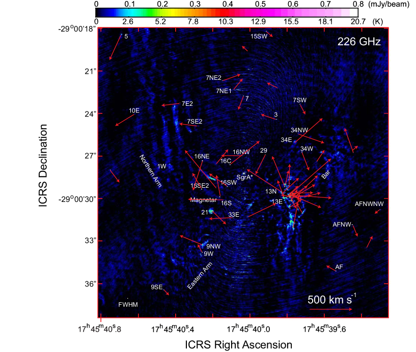
Figure 7: Proper motion referenced to Sgr A^∗ of the detected objects, which are shown as red arrows overlaid on the continuum map at 226 GHz. The angular resolution of the continuum map is $0\farcs 029\times 0\farcs 020,PA=86^{\circ}$ in FWHM, which is shown as an oval at the lower left corner.

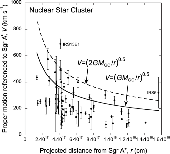
Figure 8: Relation between the proper motion and projected distance from Sgr A^∗. The solid and broken line curves show the upper limit velocities for a circular orbit around Sgr A^∗, $V=\sqrt{\frac{GM_{\mathrm{GC}}}{r_{\mathrm{peri}}}}$, and a Kepler orbit with high eccentricity, $V=\sqrt{\frac{2GM_{\mathrm{GC}}}{r_{\mathrm{peri}}}}$, respectively.

Figure 7 shows the proper motions of the detected object in the NSC as arrows overlaid on the continuum map at 226 GHz in order to explore large scale tendency of the proper motions. As mentioned above, the derived proper motions are referenced to the position of Sgr A^∗. The proper motions seem to be far from random in general. If anything, they are fairly uniform when they are in small groups, for example the IRS16, IRS13E, and IRS13N clusters. These proper motions are mostly consistent with those by IR observations (e.g. Paumard et al. (2006), Mužic et al. (2008), Schödel, Merritt,& Eckart (2009), Yelda et al. (2014)). The member stars in the IRS16 cluster seem to stream to northeast in the region southeast Sgr A^∗. Moreover, they seem to stream to northwest in the region northeast Sgr A^∗. Therefore, the member stars in the IRS16 cluster including IRS29 seem to rotate around Sgr A^∗ in clockwise. The mean rotation velocity of the cluster is estimated to be $\overline{V}=343\pm 149$ km s^-1. There may be counter clockwise motion around Sgr A^∗ in the area more distant from Sgr A^∗. Because the detected objects are sparse in the outer area, it is fairly difficult to discuss the tendency. The proper motions in IRS13E and IRS13N clusters will be discussed separately in the following subsection.

The amplitude of the proper motions is distributed in the range from $V_{\bot}=69$ km s^-1 to $V_{\bot}=690$ km s^-1. Figure 8 shows the relation between the proper motion and projected distance from Sgr A^∗. The solid and broken line curves in the figure show the upper limit of the rotation velocity for a circular orbit around Sgr A^∗, $V=\sqrt{\frac{GM_{\mathrm{GC}}}{r_{\mathrm{peri}}}}$, and the upper limit of the orbit velocity of a Kepler orbit with high eccentricity when the object is at the periastron, $V=\sqrt{\frac{2GM_{\mathrm{GC}}}{r_{\mathrm{peri}}}}$, respectively. The proper motions of almost all objects are less than the upper limit velocity for a Kepler orbit with high eccentricity. Moreover, the proper motions of many objects are less than the upper limit velocity for a circular orbit. This tendency is mostly consistent with those by IR observations (e.g. Paumard et al. (2006), Mužic et al. (2008), Schödel, Merritt,& Eckart (2009), Yelda et al. (2014)). These suggest that almost all objects are bounded by the GCBH and rotate around it. The proper motions of IRS13E1 and IRS5 are nominally larger than the upper limit velocity for a Kepler orbit with high eccentricity. The observed proper motions of IRS13E1, $V_{\mathrm{Ra}}=-520\pm 32$ km s^-1, $V_{\mathrm{Dec}}=453\pm 21$ km s^-1, is not consistent with that by IR observations (e.g. $V_{\mathrm{Ra}}=-143\pm 1$ km s^-1, $V_{\mathrm{Dec}}=-106\pm 1$ km s^-1 in Fritz et al. (2010), $V_{\mathrm{Ra}}=-195\pm 8$ km s^-1, $V_{\mathrm{Dec}}=-102\pm 5$ km s^-1 in Schödel, Merritt,& Eckart (2009)). It is not ruled out that the observed position of IRS13E1 suffers from an unavoidable artifact as mentioned previously (see Figure 9). In addition, the fitting error of IRS5 is fairly large because the object is near the edge of the FOV. Therefore these deviant proper motions would be the results of these systematic errors.

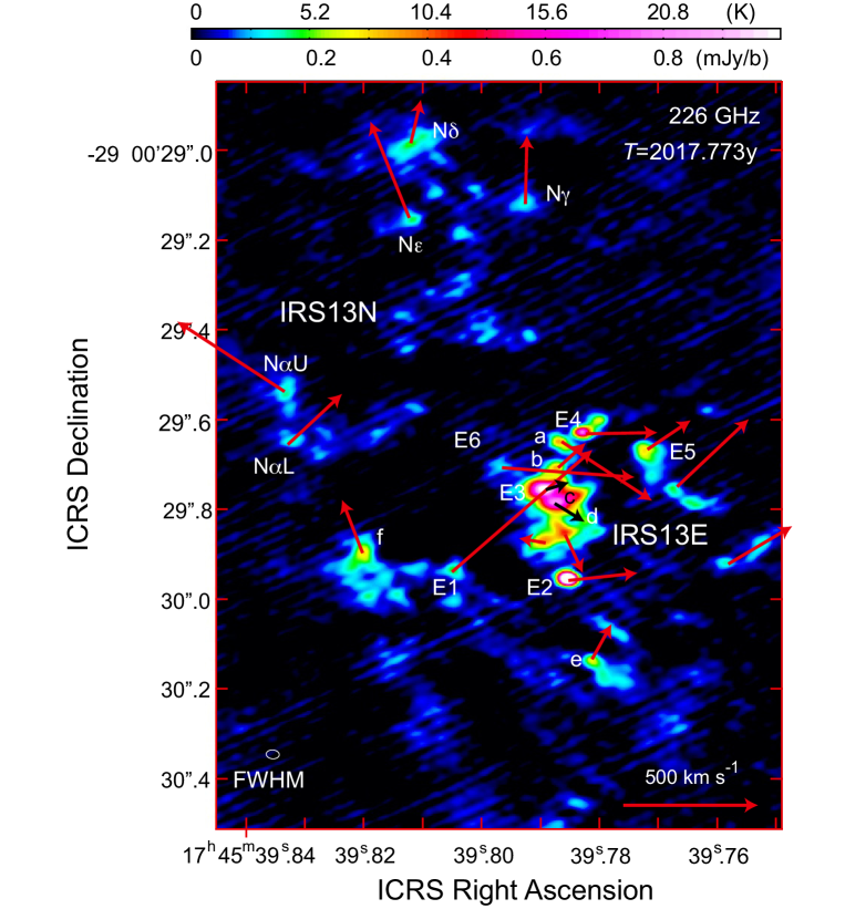
Figure 9: Proper motion of the IRS13E and IRS13N clusters, which are shown as red arrows overlaid on the enlarged continuum map at 226 GHz. The angular resolution of the continuum map is $0\farcs 029\times 0\farcs 020,PA=-86^{\circ}$ in FWHM, which is shown as an oval at the lower left corner. The mean proper motion of the IRS13E cluster except IRS13E3 and IRS13Ec are estimated to be $\overline{V_{\mathrm{Ra}}}=-218\pm 30$ km s^-1 and $\overline{V_{\mathrm{Dec}}}=73\pm 30$ km s^-1. On the other hand, the mean proper motions of the IRS13N cluster are estimated to be $\overline{V_{\mathrm{Ra}}}=60\pm 210$ km s^-1 and $\overline{V_{\mathrm{Dec}}}=274\pm 76$ km s^-1.

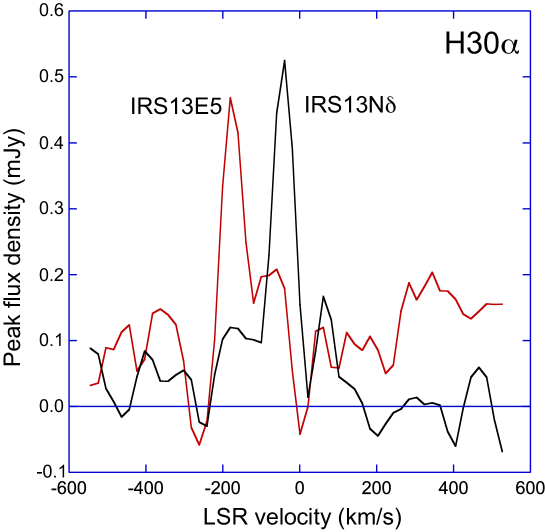
Figure 10: Line profiles toward IRS13E5 (in red) and IRS13N$\delta$ (in black) in the H30$\alpha$ recombination line. The sampling areas are ovals with the beam size, $0\farcs 037\times 0\farcs 025$, centered at IRS13E5 and IRS13N$\delta$ (see Table 1).

4.2 Proper Motion of the Member Stars of the IRS13E and IRS13N Clusters

Figure 9 is the enlarged map showing the proper motions of the member objects of the IRS13E and IRS13N clusters. These clusters seem to have peculiar proper motions (see Figure 7). Member objects of the IRS13E cluster stream monotonously to west with the velocity of $\gtrsim 200$ km s^-1. The peculiar proper motion, so called ”co-moving cluster”, has been shown by IR observations (e.g. Ott et al. (2003), Maillard et al. (2004), Schödel, Merritt,& Eckart (2009)). Although IRS13E2 and IRS13E4 are observed as WR stars certainly, IRS13E3 and IRS13Ec are thought to be gas blobs not real stars based on IR spectroscopy (e.g. Fritz et al. (2010)). The proper motions of IRS13E2 and IRS13E4 are derived to be $V_{\mathrm{Ra}}=-256\pm 3$ km s^-1, $V_{\mathrm{Dec}}=27\pm 2$ km s^-1 and $V_{\mathrm{Ra}}=-265\pm 23$ km s^-1, $V_{\mathrm{Dec}}=4\pm 14$ km s^-1, respectively. On the other hand, the values based on IR observations are $V_{\mathrm{Ra}}=-276\pm 6$ km s^-1, $V_{\mathrm{Dec}}=56\pm 8$ km s^-1 and $V_{\mathrm{Ra}}=-254\pm 7$ km s^-1, $V_{\mathrm{Dec}}=15\pm 11$ km s^-1, respectively (Schödel, Merritt,& Eckart (2009)). Our derived values are nearly equal to the IR values. The ensemble mean proper motion of the member objects except IRS13E3 and IRS13Ec are estimated to be $\overline{V_{\mathrm{Ra}}}=-218\pm 30$ km s^-1 and $\overline{V_{\mathrm{Dec}}}=73\pm 30$ km s^-1, respectively. These mean proper motions are mostly consistent with those by previous IR observations (e.g. Ott et al. (2003), Maillard et al. (2004), Schödel, Merritt,& Eckart (2009)). Although IRS13E1, IRS13E2, IRS13E4, and IRS13E6 are not detected in the H$30\alpha$ recombination line, IRS13E3, IRS13Ec and IRS13E5 are detected in the line (see Tsuboi et al. (2019b)). Figure 10 shows the line profile toward IRS13E5. Using Gaussian fit, the central velocity and FWHM velocity width of IRS13E5 are estimated to be $V_{\mathrm{C}}=-169.8\pm 4.9$ km s^-1 and $V_{\mathrm{FWHM}}=\sqrt{\Delta V_{\mathrm{obs}}^{2}-(2sampling)^{2}}=67\pm 12$ km s^-1, respectively. The FWHM velocity width is fairly wider than that of a hyper compact HII region even in the Galactic center region (e.g. Tsuboi et al. (2019b)).

The proper motions of IRS13E3 and IRS13Ec are fairly different from those of other member objects of the IRS13E cluster. The proper motions of IRS13E3 and IRS13Ec are derived to be $V_{\mathrm{Ra}}=-79\pm 27$ km s^-1, $V_{\mathrm{Dec}}=10\pm 13$ km s^-1 and $V_{\mathrm{Ra}}=-123\pm 18$ km s^-1, $V_{\mathrm{Dec}}=-48\pm 11$ km s^-1, respectively. The derived proper motions of IRS13E3 are nearly equal to those by IR observations (e.g. $V_{\mathrm{Ra}}=-105\pm 23$ km s^-1, $V_{\mathrm{Dec}}=-16\pm 27$ km s^-1 in Schödel, Merritt,& Eckart (2009), $V_{\mathrm{Ra}}=-82\pm 9$ km s^-1, $V_{\mathrm{Dec}}=8\pm 9$ km s^-1 in Fritz et al. (2010), $V_{\mathrm{Ra}}=-97\pm 18$ km s^-1, $V_{\mathrm{Dec}}=-14\pm 15$ km s^-1in Eckart et al. (2013)). However, the proper motion of IRS13Ec is not derived by IR observations because the IR counterpart of IRS13Ec is not clearly detected (e.g. see Figure 2 in Fritz et al. (2010)). Although IRS13E2 and IRS13E4 are located southeast and north of IRS13E3 in the IR map observed over 10 years ago (e.g. see Figure 2 in Fritz et al. (2010)), they are located southwest and northwest of IRS13E3 in 2017 map as shown in Figure 9. The similar positional change is also seen in the relation between IRS13E3 and IRS13E5. These are consistent with that the proper motion of IRS13E3 is fairly smaller than those of IRS13E2, IRS13E4 and IRS13E5. The dissimilarity of the proper motions of IRS13E3 and IRS13Ec from the rest of IRS13 cluster member objects suggests that they are not member objects of the cluster. Although the radial velocity analysis of the ionized gas in IRS13E3 has been published (Tsuboi et al. (2017b), Tsuboi et al. (2019a)), the joint analysis of the radial velocity and proper motion will be discussed in another upcoming paper.

The member objects of the IRS13N cluster have been identified in radio (e.g. Yusef-Zadeh et al. (2014)) and IR observations (e.g. Mužic et al. (2008), Eckart et al. (2013)). The objects of the IRS13N cluster also seem to stream monotonously to north with the velocity of $\gtrsim 200$ km s^-1 as shown in Figure 9 and Table 3. The co-moving property toward north of the IRS13N cluster had been found in IR observations (e.g. Mužic et al. (2008)). The ensemble mean proper motions of the member stars are estimated to be $\overline{V_{\mathrm{Ra}}}=60\pm 210$ km s^-1 and $\overline{V_{\mathrm{Dec}}}=274\pm 76$ km s^-1. IRS13N$\delta$ is also detected as a single peak line profile object in the H$30\alpha$ recombination line (see Figure 9). Other member objects shown in Table 3 is not detected in the H$30\alpha$ recombination line. Using Gaussian fit, the central velocity and FWHM velocity width of IRS13N$\delta$ are estimated to be $V_{\mathrm{C}}=-43.1\pm 2.3$ km s^-1 and $V_{\mathrm{FWHM}}=\sqrt{\Delta V_{\mathrm{obs}}^{2}-(2sampling)^{2}}=59\pm 16$ km s^-1, respectively. As in the case of IRS13E5, the FWHM velocity width of IRS13N$\delta$ is also wider than that of a hyper compact HII region (e.g. Tsuboi et al. (2019b)).

5 Conclusions

We have observed Sgr A^∗ and the surrounding area including the NSC at 230 GHz with ALMA in October 2017 and analyzed the data. We also analyzed the similar ALMA archive data obtained in June 2019. The angular resolution in the both resultant maps is $\sim 0\farcs 03$. We determined the positions relative to Sgr A^∗ of 65 compact objects on the resultant map of October 2017 using 2-D Gaussian fit. The positional accuracy is as high as $\sim 0\farcs 001$. We also determined the relative positions of 64 objects on the resultant map of June 2019. We derived the proper motions relative to Sgr A^∗ of the 64 objects by comparing these relative positions. The derived proper motions are roughly described with both clockwise and counterclockwise rotations around Sgr A^∗. The rotation velocities are reproduced by Kepler orbits bounded around Sgr A^∗. Moreover, the proper motions include co-moving clusters for example IRS13E and IRS13N. These positions and proper motions are almost consistent with those by previous infrared observations. Therefore the demonstrations prove that ALMA is a powerful tool for precision astrometry of this region. This work is supported in part by the Grant-in-Aid from the Ministry of Education, Sports, Science and Technology (MEXT) of Japan, No.19K03939. The National Radio Astronomy Observatory (NRAO) is a facility of the National Science Foundation operated under cooperative agreement by Associated Universities, Inc. USA. ALMA is a partnership of ESO (representing its member states), NSF (USA) and NINS (Japan), together with NRC (Canada), NSC and ASIAA (Taiwan), and KASI (Republic of Korea), in cooperation with the Republic of Chile. The Joint ALMA Observatory (JAO) is operated by ESO, AUI/NRAO and NAOJ. This paper makes use of the following ALMA data: ADS/JAO.ALMA#2015.1.01080.S, ALMA#2017.1.00503.S, and #2018.1.001124.S.

References

- Andrews et al. (2019) Andrews, H., Fenech, D., Prinja, R. K., Clark, J. S., & Hindson, L. 2019, A&A, 632, id. A38
- Gravity Collaboration (2018) Gravity Collaboration; Abuter, R. et al. 2018, A&A, 615, L15
- Boehle et al. (2016) Boehle, A. et al. 2016, ApJ, 830, id 17
- Cappa et al. (2004) Cappa, C., Goss, W. M., & van der Hucht, K. A. 2004, AJ, 127, 2885
- Condon (1997) Condon, J. J., 1997, PASP, 109, 166
- Cotton (1999) Cotton, W. D. 1999, Synthesis Imaging in Radio Astronomy II, eds. G. B. Taylor, C. L. Carilli, and R. A. Perley (San Francisco, CA, USA), ASP Conference Series, 180, 357
- Eckart et al. (2013) Eckart, A. et al. 2013, A&A, 551, A18
- Figer et al. (1999) Figer, D. F.; McLean, I. S., & Morris, M., 1999, ApJ, 514, 202
- Figer et al. (2002) Figer, D. F. Najarro, F., Gilmore, D., Morris, et al. 2002, ApJ, 581, 258
- Fritz et al. (2010) Fritz, T. K. et al. 2010, ApJ, 721, 395
- Genzel et al. (1996) Genzel, R., Thatte, N., Krabbe, A., Kroker, H., & Tacconi-Garman, L. E. 1996, ApJ, 472, 153
- Genzel et al. (2010) Genzel, R., Eisenhauer, F., & Gillessen, S. 2010, Rev. Mod. Phys, 82, 3121
- Ghez et al. (2008) Ghez, A. M., et al. 2008, ApJ, 689, 1044
- Iwata et al. (2020) Iwata, Y., Oka, T., Tsuboi, M., Miyoshi, M., & Takekawa, S., 2020, ApJ, 892, id. L30
- Maillard et al. (2004) Maillard, J. P.; Paumard, T.; Stolovy, S. R.; Rigaut, F. 2004, A&A, 423, 155
- McMullin et al. (2007) McMullin, J. P., Waters, B., Schiebel, D., Young, W., & Golap, K. 2007, Astronomical Data Analysis Software and Systems XVI, eds. R. A. Shaw, F. Hill, & D. J. Bell (San Francisco, CA, USA), ASP Conference Series, 376, 127
- Miyazaki, Tsutsumi & Tsuboi (2004) Miyazaki, A., Tsutsumi, T., & Tsuboi, M. 2004, ApJ, 423, 155
- Murchikova & Witzel (2020) Murchikova, L. & Witzel, G. 2021, arXiv:2107.11391
- Mužic et al. (2008) Mužic, K., Schödel, R., Eckart , A., Meyer, L., & Zensus, A. 2008, A&A, 482,173
- Ott et al. (2003) Ott, T., Genzel, R., Eckart, A., & Schödel, R. 2003, GC02 Workshop, Astron. Nachr., 324/S1, 543
- Paumard et al. (2006) Paumard, T., et al. 2006, ApJ, 643, 1011
- Rau (2012) Rau, U., 2012, Image Reconstruction from Incomplete Data VII. (San Diego, CA, USA), Proceedings of the SPIE, 8500, id. 85000N
- Schödel, Merritt,& Eckart (2009) Schödel, R., Merritt, D.& Eckart, A., 2009, A&A, 502, 91
- Tsuboi et al. (2017a) Tsuboi, M., Kitamura, Y., Uehara, K., Miyawaki, R., Tsutsumi, T., Miyazaki, A., & Miyoshi, M., 2017a, ApJ, 824, id. 94
- Tsuboi et al. (2017b) Tsuboi, M., Kitamura, Y., Tsutsumi, T., Uehara, K., Miyoshi, M., Miyawaki, R., & Miyazaki, A., 2017b, ApJ, 850, id L5
- Tsuboi et al. (2019a) Tsuboi, M., Kitamura, Y., Tsutsumi, T., Miyawaki, R., Miyoshi, M., & Miyazaki, A., 2019a, PASJ, 71, id 105
- Tsuboi et al. (2019b) Tsuboi, M., Kitamura, Y., Uehara, K., Miyazaki, A., Miyawaki, R., Tsutsumi, T., & Miyoshi, M., 2019, PASJ, 71, id 128
- Yusef-Zadeh et al. (2014) Yusef-Zadeh, F., Roberts, D. A., Bushouse, H., Wardle, M., Cotton, W., Royster, M., & van Moorsel, G., 2014, ApJ, 792, L1
- Yelda et al. (2014) Yelda, S., Ghez, A. M., Lu, J. R., et al. 2014, ApJ, 783, 131
- Zhao et al. (2009) Zhao, J.-H., Morris, M. R., Goss, W. M., & An, T., 2009, ApJ, 699,186