Control-oriented meta-learning

Abstract

Real-time adaptation is imperative to the control of robots operating in complex, dynamic environments. Adaptive control laws can endow even nonlinear systems with good trajectory tracking performance, provided that any uncertain dynamics terms are linearly parameterizable with known nonlinear features. However, it is often difficult to specify such features a priori, such as for aerodynamic disturbances on rotorcraft or interaction forces between a manipulator arm and various objects. In this paper, we turn to data-driven modeling with neural networks to learn, offline from past data, an adaptive controller with an internal parametric model of these nonlinear features. Our key insight is that we can better prepare the controller for deployment with control-oriented meta-learning of features in closed-loop simulation, rather than regression-oriented meta-learning of features to fit input-output data. Specifically, we meta-learn the adaptive controller with closed-loop tracking simulation as the base-learner and the average tracking error as the meta-objective. With both fully-actuated and underactuated nonlinear planar rotorcraft subject to wind, we demonstrate that our adaptive controller outperforms other controllers trained with regression-oriented meta-learning when deployed in closed-loop for trajectory tracking control.

1 Introduction

Figure 1: While roboticists can often derive a model for how control inputs affect the system state, it is much more difficult to model prevalent external forces (e.g., from aerodynamics, contact, and friction) that adversely affect tracking performance. In this work, we present a method to meta-learn an adaptive controller offline from previously collected data. Our meta-learning is control-oriented rather than regression-oriented; specifically, we: 1) collect input-output data on the true system, 2) train a parametric adaptive controller in closed-loop simulation to adapt well to each model of an ensemble constructed from past input-output data, and 3) test our adaptive controller on the real system. Our method contextualizes training within the downstream control objective, thereby engendering good tracking results at test time, which we demonstrate on fully-actuated and underactuated versions of a planar quadrotor system subject to wind.

Performant control in robotics is impeded by the complexity of the dynamical system consisting of the robot itself (i.e., its nonlinear equations of motion) and the interactions with its environment. Roboticists can often derive a physics-based robot model, and then choose from a suite of nonlinear control laws that each offer desirable control-theoretic properties (e.g., good tracking performance) in known, simple environments. Even in the face of model uncertainty, nonlinear control can still yield such properties with the help of real-time adaptation to online measurements, provided the uncertainty enters the system in a known, structured manner.

However, when a robot is deployed in complex scenarios, it is generally intractable to know even the structure of all possible configurations and interactions that the robot may experience. To address this, system identification and data-driven control seek to learn an accurate input-output model from past measurements. Recent years have also seen a dramatic proliferation of research in machine learning for control by leveraging powerful approximation architectures to predict and optimize the behaviour of dynamical systems. In general, such rich models require extensive data and computation to back-propagate gradients for many layers of parameters, and thus usually cannot be used in fast nonlinear control loops.

Moreover, machine learning of dynamical system models often prioritizes fitting input-output data, i.e., it is regression-oriented, with the rationale that designing a controller for a highly accurate model engenders better closed-loop performance on the real system. However, decades of work in system identification and adaptive control recognize that, since a model is often learned for the purpose of control, the learning process itself should be tailored to the downstream control objective. This concept of control-oriented learning is exemplified by fundamental results in adaptive control theory; guarantees on tracking convergence can be attained without convergence of the parameter estimates to those of the true system.

1.1 Contributions

In this work, we acknowledge this distinction between regression-oriented and control-oriented learning, and propose a control-oriented method to learn a parametric adaptive controller that performs well in closed-loop at test time. Critically, our method (outlined in Figure 1) focuses on offline learning from past trajectory data. We formalize training the adaptive controller as a semi-supervised, bi-level meta-learning problem, with the average integrated tracking error across chosen target trajectories as the meta-objective. We use a closed-loop simulation with our adaptive controller as a base-learner, which we then back-propagate gradients through. We discuss how our formulation can be applied to adaptive controllers for general dynamical systems, then specialize it to different classes of nonlinear systems. Through our experiments, we show that by injecting the downstream control objective into offline meta-learning of an adaptive controller, we improve closed-loop trajectory tracking performance at test time in the presence of widely varying disturbances. We provide code to reproduce our results at https://github.com/StanfordASL/Adaptive-Control-Oriented-Meta-Learning.

A preliminary version of this article was presented at Robotics: Science and Systems 2021 (Richards et al., 2021). In this revised and extended version, we additionally contribute: 1) exposition on how our meta-learning framework can be applied to control-affine and underactuated nonlinear systems, 2) analysis of the relationship between stability certificate functions and online adaptation laws for stable concurrent learning and control, 3) new experiments on an underactuated aerial vehicle system that reinforce our previous observations for fully-actuated systems, and 4) additional experiments with unknown time-varying disturbances.

2 Related Work

In this section, we review three key areas of work related to this paper: control-oriented system identification, adaptive control, and meta-learning.

2.1 Control-Oriented System Identification

Learning a system model for the express purpose of closed-loop control has been a hallmark of linear system identification since at least the early 1970s (Åström and Wittenmark, 1971). Due to the sheer amount of literature in this area, we direct readers to the book by Ljung (1999) and the survey by Gevers (2005). Some salient works are the demonstrations by Skelton (1989) on how large open-loop modelling errors do not necessarily cause poor closed-loop prediction, and the theory and practice from Hjalmarsson et al. (1996) and Forssell and Ljung (2000) for iterative online closed-loop experiments that encourage convergence to a model with optimal closed-loop behaviour. In this paper, we focus on offline meta-learning targeting a downstream closed-loop control objective, to train adaptive controllers for nonlinear systems.

In nonlinear system identification, there is an emerging body of literature on data-driven, constrained learning for dynamical systems that encourages learned models and controllers to perform well in closed-loop. Khansari-Zadeh and Billard (2011) and Medina and Billard (2017) train controllers to imitate known invertible dynamical systems while constraining the closed-loop system to be stable. Chang et al. (2019) and Sun et al. (2020) jointly learn a controller and a stability certificate for known dynamics to encourage good performance in the resulting closed-loop system. Singh et al. (2020) jointly learn a dynamics model and a stabilizability certificate that regularizes the model to perform well in closed-loop, even with a controller designed a posteriori. Overall, these works concern learning a fixed model-controller pair. Instead, with offline meta-learning, we train an adaptive controller that can update its internal representation of the dynamics online. We discuss future work explicitly incorporating stability constraints in Section 8.

2.2 Adaptive Control

Broadly speaking, adaptive control concerns parametric controllers paired with an adaptation law that dictates how the parameters are adjusted online in response to signals in a dynamical system (Slotine and Li, 1991; Narendra and Annaswamy, 2005; Landau et al., 2011; Ioannou and Sun, 2012). Since at least the 1950s, researchers in adaptive control have focused on parameter adaptation prioritizing control performance over parameter identification (Aseltine et al., 1958). Indeed, one of the oldest adaptation laws, the so-called MIT rule, is essentially gradient descent on the integrated squared tracking error (Mareels et al., 1987). Tracking convergence to a reference signal is the primary result in Lyapunov stability analyses of adaptive control designs (Narendra and Valavani, 1978; Narendra et al., 1980), with parameter convergence as a secondary result if the reference is persistently exciting (Anderson and Johnson, 1982; Boyd and Sastry, 1986). In the absence of persistent excitation, Boffi and Slotine (2021) show certain adaptive controllers also “implicitly regularize” (Azizan and Hassibi, 2019; Azizan et al., 2021) the learned parameters to have small Euclidean norm; moreover, different forms of implicit regularization (e.g., sparsity-promoting) can be achieved by certain modifications of the adaptation law. Overall, adaptive control prioritizes control performance while learning parameters on a “need-to-know” basis, which is a principle that can be extended to many learning-based control contexts (Wensing and Slotine, 2020).

Stable adaptive control of nonlinear systems often relies on linearly parameterizable dynamics with known nonlinear basis functions, i.e., features, and the ability to cancel these nonlinearities stably with the control input when the parameters are known exactly (Slotine and Li, 1987, 1989, 1991; Lopez and Slotine, 2020). When such features cannot be derived a priori, function approximators such as neural networks (Sanner and Slotine, 1992; Joshi and Chowdhary, 2019; Joshi et al., 2020), Gaussian processes (Grande et al., 2013; Gahlawat et al., 2020), and random Fourier features (Boffi et al., 2021) can be used and updated online in the adaptive control loop. However, fast closed-loop adaptive control with complex function approximators is hindered by the computational effort required to train them; this issue is exacerbated by the practical need for controller gain tuning. In our paper, we focus on offline meta-training of neural network features and controller gains from collected data, with controller structures that can operate in fast closed-loops.

2.3 Meta-Learning

Meta-learning is the tool we use to inject the downstream adaptive control application into offline learning from data. Informally, meta-learning or “learning to learn” improves knowledge of how to best optimize a given meta-objective across different tasks. In the literature, meta-learning has been formalized in various manners; we refer readers to Hospedales et al. (2021) for a survey of them. In general, the algorithm chosen to solve a specific task is the base-learner, while the algorithm used to optimize the meta-objective is the meta-learner. In our work, when trying to make a dynamical system track several target trajectories, each trajectory is associated with a “task”, the adaptive tracking controller is the base-learner, and the average tracking error across all of these trajectories is the meta-objective we want to minimize.

Many works try to meta-learn a dynamics model offline that can best fit new input-output data gathered during a particular task. That is, the base- and meta-learners are regression-oriented. Bertinetto et al. (2019) and Lee et al. (2019) back-propagate through closed-form ridge regression solutions for few-shot learning, with a maximum likelihood meta-objective. O’Connell et al. (2021) apply this same method to learn neural network features for nonlinear mechanical systems. Harrison et al. (2018b, a) more generally back-propagate through a Bayesian regression solution to train a Bayesian prior dynamics model with nonlinear features. Nagabandi et al. (2019) use a maximum likelihood meta-objective, and gradient descent on a multi-step likelihood objective as the base-learner. Belkhale et al. (2021) also use a maximum likelihood meta-objective, albeit with the base-learner as a maximization of the Evidence Lower BOund (ELBO) over parameterized, task-specific variational posteriors; at test time, they perform latent variable inference online in a slow control loop.

Finn et al. (2017); Rajeswaran et al. (2017), and Clavera et al. (2018) meta-train a policy with the expected accumulated reward as the meta-objective, and a policy gradient step as the base-learner. These works are similar to ours in that they infuse offline learning with a more control-oriented flavour. However, while policy gradient methods are amenable to purely data-driven models, they beget slow control-loops due to the sampling and gradients required for each update. Instead, we back-propagate gradients through offline closed-loop simulations to train adaptive controllers designed for fast online implementation. This yields a meta-trained adaptive controller that enjoys the performance of principled design inspired by the rich body of control-theoretical literature.

3 Problem Statement

In this paper, we are interested in controlling the continuous-time, nonlinear dynamical system

$$\dot{x}=f(x,u,w),$$ (1)

where $x(t)\in\mathbb{R}^{n}$ is the state, $u(t)\in\mathbb{R}^{m}$ is the control input, and $w(t)\in\mathbb{R}^{d}$ is some unknown disturbance, each at time $t\in\mathbb{R}_{\geq 0}$. Specifically, for a given target trajectory $x^{*}(t)\in\mathbb{R}^{n}$, we want to choose $u(t)$ such that $x(t)$ converges to $x^{*}(t)$; we then say $u(t)$ makes the system 1 track $x^{*}(t)$.

Since $w(t)$ is unknown and possibly time-varying, we want to design a feedback law $u=\pi(x,x^{*},\hat{a})$ with parameters $\hat{a}(t)$ that are updated online according to a chosen adaptation law $\dot{\hat{a}}=\rho(x,x^{*},\hat{a})$. We refer to $(\pi,\rho)$ together as an adaptive controller. For example, consider the control-affine system

$$\dot{x}=f(x)+B(x)(u+Y(x)a),$$ (2)

where $f$, $B$, and $Y$ are known, possibly nonlinear maps, and $a$ is a vector of unknown parameters. We can interpret ${w(t)=Y(x(t))a}$ as the disturbance in this system. A reasonable feedback law choice would be

$$u=\bar{\pi}(x,x^{*})-Y(x)\hat{a},$$ (3)

where $\bar{\pi}$ ensures ${\dot{x}=f(x)+B(x)\bar{\pi}(x,x^{*})}$ tracks $x^{*}(t)$, and the term $Y(x)\hat{a}$ is meant to cancel $Y(x)a$ in 2. For this reason, $Y(x)a$ is termed a matched uncertainty in the literature. If the adaptation law $\dot{\hat{a}}=\rho(x,x^{*},\hat{a})$ is designed such that $Y(x(t))\hat{a}(t)$ converges to $Y(x(t))a(t)$, then we can use 3 to make 2 track $x^{*}(t)$. Critically, this is not the same as requiring $\hat{a}(t)$ to converge to $a(t)$. Since $Y(x)a$ depends on $x(t)$ and hence indirectly on the target $x^{*}(t)$, the roles of feedback and adaptation are inextricably linked by the tracking control objective. Overall, learning in adaptive control is done on a “need-to-know” basis to cancel $Y(x)a$ in closed-loop, rather than to estimate $a$ in open-loop.

4 Bi-Level Meta-Learning

We now describe some preliminaries on meta-learning akin to Finn et al. (2017) and Rajeswaran et al. (2019), so that we can apply these ideas in the next section to the adaptive control problem 1 and in Section 7.3 to our baselines.

In machine learning, we typically seek some optimal parameters ${\xi^{*}\in\operatorname*{\mathrm{arg\,min}}_{\xi}\ell(\xi,\mathcal{D})}$, where $\ell$ is a scalar-valued loss function and $\mathcal{D}$ is some data set. In meta-learning, we instead have a collection of loss functions $\{\ell_{i}\}_{i=1}^{M}$, training data sets $\{\mathcal{D}^{\mathrm{train}}_{i}\}_{i=1}^{M}$, and evaluation data sets $\{\mathcal{D}^{\mathrm{eval}}_{i}\}_{i=1}^{M}$, where each $i$ corresponds to a task. Moreover, during each task $i$, we can apply an adaptation mechanism ${\operatorname{\mathrm{Adapt}}:(\theta,\mathcal{D}^{\mathrm{train}}_{i})\mapsto\xi_{i}}$ to map so-called meta-parameters $\theta$ and the task-specific training data $\mathcal{D}^{\mathrm{train}}_{i}$ to task-specific parameters $\xi_{i}$. The crux of meta-learning is to solve the bi-level problem

$$\begin{aligned} \theta^{*}\in\,&\operatorname*{\mathrm{arg\,min}}_{\theta}\frac{1}{M}\left(\sum_{i=1}^{M}\ell_{i}(\xi_{i},\mathcal{D}_{i}^{\mathrm{eval}})+\mu_{\mathrm{meta}}\lVert\theta\rVert_{2}^{2}\right)\\ &\ \mathrm{s.t.}\enspace\xi_{i}=\operatorname{\mathrm{Adapt}}(\theta,\mathcal{D}^{\mathrm{train}}_{i})\end{aligned},$$ (4)

with regularization coefficient $\mu_{\mathrm{meta}}\geq 0$, thereby producing meta-parameters $\theta^{*}$ that are on average well-suited to being adapted for each task. This motivates the moniker “learning to learn” for meta-learning. The optimization 4 is the meta-problem, while the average loss is the meta-loss. The adaptation mechanism $\mathrm{Adapt}$ is termed the base-learner, while the algorithm used to solve 4 is termed the meta-learner (Hospedales et al., 2021).

Generally, the meta-learner is chosen to be some gradient descent algorithm. Choosing a good base-learner is an open problem in meta-learning research. Finn et al. (2017) propose using a gradient descent step as the base-learner, such that $\xi_{i}=\theta-\alpha\operatorname{\nabla\!}_{\theta}\ell_{i}(\theta,\mathcal{D}_{i}^{\mathrm{train}})$ in 4 with some learning rate ${\alpha>0}$. This approach is general in that it can be applied to any differentiable task loss functions. Bertinetto et al. (2019) and Lee et al. (2019) instead study when the base-learner can be expressed as a convex program with a differentiable closed-form solution. In particular, they consider ridge regression with the hypothesis $\hat{y}=Ag(x;\theta)$, where $A$ is a matrix and $g(x;\theta)$ is some vector of nonlinear features parameterized by $\theta$. For the base-learner, they use

$$\xi_{i}=\operatorname*{\mathrm{arg\,min}}_{A}\sum_{(x,y)\in\mathcal{D}_{i}^{\mathrm{train}}}\lVert y-Ag(x;\theta)\rVert_{2}^{2}+\mu_{\mathrm{ridge}}\lVert A\rVert_{F}^{2},$$ (5)

with regularization coefficient $\mu_{\mathrm{ridge}}>0$ for the Frobenius norm $\lVert A\rVert_{F}^{2}$, which admits a differentiable, closed-form solution. Instead of adapting $\theta$ to each task $i$ with a single gradient step, this approach leverages the convexity of ridge regression tasks to minimize the task loss analytically.

5 Adaptive Control as a Base-Learner

We now present the key idea of our paper, which uses meta-learning concepts introduced in Section 4 to tackle the problem of learning to control 1. For the moment, we assume we can simulate the dynamics function $f$ in 1 offline and that we have $M$ samples $\{w_{j}(t)\}_{j=1}^{M}$ for $t\in[0,T]$ in 1; we will eliminate these assumptions in Section 5.2.

5.1 Meta-Learning from Feedback and Adaptation

In meta-learning vernacular, we treat a target trajectory $x^{*}_{i}(t)\in\mathbb{R}^{n}$ and disturbance signal $w_{j}(t)\in\mathbb{R}^{d}$ together over some time horizon $T>0$ as the training data ${\mathcal{D}_{ij}^{\mathrm{train}}=\{x^{*}_{i}(t),w_{j}(t)\}_{t\in[0,T]}}$ for task $(i,j)$. We wish to learn the static, possibly shared parameters $\theta$ of an adaptive controller

$$\begin{aligned} u&=\pi(x,x^{*},\hat{a};\theta)\\ \dot{\hat{a}}&=\rho(x,x^{*},\hat{a};\theta)\end{aligned}~{},$$ (6)

such that $(\pi,\rho)$ engenders good tracking of $x^{*}_{i}(t)$ for ${t\in[0,T]}$ subject to the disturbance $w_{j}(t)$. Our adaptation mechanism is the forward-simulation of our closed-loop system, i.e., in 4 we have $\xi_{ij}=\{x_{ij}(t),\hat{a}_{ij}(t),u_{ij}(t)\}_{t\in[0,T]}$, where

$$x_{ij}(t) =x_{ij}(0)+\int_{0}^{T}f(x_{ij}(t),u_{ij}(t),w_{j}(t))\,dt,$$ (7)

$$\hat{a}_{ij}(t) =\hat{a}_{ij}(0)+\int_{0}^{T}\rho(x_{ij}(t),x^{*}_{i}(t),\hat{a}_{ij}(t);\theta)\,dt,$$

$$u_{ij}(t) =\pi(x_{ij}(t),x^{*}_{i}(t),\hat{a}_{ij}(t);\theta),$$

which we can compute with any Ordinary Differential Equation (ODE) solver. For simplicity, we always set $x_{ij}(0)=x^{*}_{i}(0)$ and $a_{ij}(0)=0$. Our task loss is simply the average tracking error for the same target-disturbance pair, i.e., $\mathcal{D}_{ij}^{\mathrm{eval}}=\{x^{*}_{i}(t),w_{j}(t)\}_{t\in[0,T]}$ and

$$\ell_{ij}(\xi_{ij},\mathcal{D}_{ij}^{\mathrm{eval}})=\frac{1}{T}\int_{0}^{T}\left(\lVert x_{ij}(t)-x^{*}_{i}(t)\rVert_{2}^{2}+\mu_{\mathrm{ctrl}}\lVert u_{ij}(t)\rVert_{2}^{2}\right)\,dt,$$ (8)

where $\mu_{\mathrm{ctrl}}\geq 0$ regularizes the average control effort $\frac{1}{T}\int_{0}^{T}\lVert u_{ij}(t)\rVert_{2}^{2}\,dt$. This loss is inspired by the Linear Quadratic Regulator (LQR) from optimal control, and can be generalized to weighted norms. Suppose we construct $N$ target trajectories $\{x^{*}_{i}(t)\}_{i=1}^{N}$ and sample $M$ disturbance signals $\{w_{j}(t)\}_{j=1}^{M}$, thereby creating $NM$ tasks. Combining 7 and 8 for all $(i,j)$ in the form of 4 then yields the meta-problem

$$\begin{aligned} \min_{\theta}\ &\frac{1}{NMT}\left(\sum_{i=1}^{N}\sum_{j=1}^{M}\int_{0}^{T}c_{ij}(t)\,dt+\mu_{\mathrm{meta}}\lVert\theta\rVert_{2}^{2}\right)\\ &\mathrm{s.t.}\enspace\begin{aligned} c_{ij}&=\lVert x_{ij}-x^{*}_{i}\rVert_{2}^{2}+\mu_{\mathrm{ctrl}}\lVert u_{ij}\rVert_{2}^{2}\\ \dot{x}_{ij}&=f(x_{ij},u_{ij},w_{j}),\ x_{ij}(0)=x^{*}_{i}(0)\\ \dot{\hat{a}}_{ij}&=\rho(x_{ij},x^{*}_{i},\hat{a}_{ij};\theta),\ \hat{a}_{ij}(0)=0\\ u_{ij}&=\pi(x_{ij},x^{*}_{i},\hat{a}_{ij};\theta)\end{aligned}\end{aligned}.$$ (9)

Solving 9 would yield parameters $\theta$ for the adaptive controller $(\pi,\rho)$ such that it works well on average in closed-loop tracking of $\{x^{*}_{i}(t)\}_{i=1}^{N}$ for the dynamics $f$, subject to the disturbances $\{w_{j}(t)\}_{j=1}^{M}$. To learn the meta-parameters $\theta$, we can perform gradient descent on 9. This requires back-propagating through an ODE solver, which can be done either directly or via the adjoint state method after solving the ODE forward in time (Pontryagin et al., 1962; Chen et al., 2018; Andersson et al., 2019; Millard et al., 2020). In addition, the learning problem 9 is semi-supervised, in that $\{w_{j}(t)\}_{j=1}^{M}$ are labelled samples and $\{x^{*}_{i}(t)\}_{i=1}^{N}$ can be chosen freely. If there are some specific target trajectories we want to track at test time, we can use them in the meta-problem 9. This is an advantage of designing the offline learning problem in the context of the downstream control objective.

5.2 Model Ensembling as a Proxy for Feedback Offline

In practice, we cannot simulate the true dynamics $f$ or sample an actual disturbance trajectory $w(t)$ offline. Instead, we can more reasonably assume we have past data collected with some other, possibly poorly tuned controller. In particular, we assume access to trajectory data $\{\mathcal{T}_{j}\}_{j=1}^{M}$, such that

$$\mathcal{T}_{j}\coloneqq\big{\{}\big{(}t^{(k)}_{j},x^{(k)}_{j},u^{(k)}_{j},t^{(k+1)}_{j},x^{(k+1)}_{j}\big{)}\big{\}}_{k=0}^{N_{j}-1},$$ (10)

where $x^{(k)}_{j}\coloneqq x_{j}(t^{(k)}_{j})$ and $u^{(k)}_{j}\coloneqq u_{j}(t^{(k)}_{j})$ were the state and control input, respectively, at time $t^{(k)}_{j}$.

Inspired by Clavera et al. (2018), since we cannot simulate the true dynamics $f$ offline, we propose to first train a model ensemble from the trajectory data $\{\mathcal{T}_{j}\}_{j=1}^{M}$ to roughly capture the distribution of $f(\cdot,\cdot,w)$ over possible values of the disturbance $w$. Specifically, we fit a model $\hat{f}_{j}(x,u;\psi_{j})$ with parameters $\psi_{j}$ to each trajectory $\mathcal{T}_{j}$, and use this as a proxy for $f(x,u,w_{j})$ in 9. The meta-problem 9 is now

$$\min_{\theta} \frac{1}{NMT}\left(\sum_{i=1}^{N}\sum_{j=1}^{M}\int_{0}^{T}c_{ij}(t)\,dt+\mu_{\mathrm{meta}}\lVert\theta\rVert_{2}^{2}\right)$$ (11)

$$\mathrm{s.t.}\enspace\begin{aligned} c_{ij}&=\lVert x_{ij}-x^{*}_{i}\rVert_{2}^{2}+\mu_{\mathrm{ctrl}}\lVert u_{ij}\rVert_{2}^{2}\\ \dot{x}_{ij}&=\hat{f}_{j}(x_{ij},u_{ij};\psi_{j}),\ x_{ij}(0)=x^{*}_{i}(0)\\ \dot{\hat{a}}_{ij}&=\rho(x_{ij},x^{*}_{i},\hat{a}_{ij};\theta),\ \hat{a}_{ij}(0)=0\\ u_{ij}&=\pi(x_{ij},x^{*}_{i},\hat{a}_{ij};\theta)\end{aligned}$$

This form is still semi-supervised, since each model $\hat{f}_{j}$ is dependent on the trajectory data $\mathcal{T}_{j}$, while $\{x^{*}_{i}\}_{i=1}^{N}$ can be chosen freely. The collection $\{\hat{f}_{j}\}_{j=1}^{M}$ is termed a model ensemble. Empirically, the use of model ensembles has been shown to improve robustness to model bias and train-test data shift of deep predictive models (Lakshminarayanan et al., 2017) and policies in reinforcement learning (Rajeswaran et al., 2017; Kurutach et al., 2018; Clavera et al., 2018). To train the parameters $\psi_{j}$ of model $\hat{f}_{j}$ on the trajectory data $\mathcal{T}_{j}$, we do gradient descent on the one-step prediction problem

$$\min_{\psi_{j}} \frac{1}{N_{j}}\left(\sum_{k=0}^{N_{j}-1}\big{\lVert}x_{j}^{(k+1)}-\hat{x}_{j}^{(k)}\big{\rVert}_{2}^{2}+\mu_{\mathrm{ensem}}\lVert\psi_{j}\rVert_{2}^{2}\right)$$ (12)

$$\mathrm{s.t.}\enspace\begin{aligned} \hat{x}_{j}^{(k+1)}&=x_{j}^{(k)}+\int_{t_{j}^{(k)}}^{t_{j}^{(k+1)}}\hat{f}_{j}(x(t),u_{j}^{(k)};\psi_{j})\,dt\end{aligned}$$

where $\mu_{\mathrm{ensem}}>0$ regularizes $\psi_{j}$. Since we meta-train $\theta$ in 12 to be adaptable to every model in the ensemble, we only need to roughly characterize how the dynamics $f(\cdot,\cdot,w)$ vary with the disturbance $w$, rather than do exact model fitting of $\hat{f}_{j}$ to $\mathcal{T}_{j}$. Thus, we approximate the integral in 12 with a single step of a chosen ODE integration scheme and back-propagate through this step, rather than use a full pass of an ODE solver.

6 Incorporating Prior Knowledge About Robot Dynamics for Principled Control-Oriented Meta-Learning

So far our method has been agnostic to the choice of adaptive controller $(\pi,\rho)$. However, if we have some prior knowledge of the dynamical system 1, we can use this to make a good choice of structure for $(\pi,\rho)$. In Sections 6.1 and 6.2, we review adaptive control designs for two general classes of nonlinear dynamical systems. Then, in Section 6.3 we discuss how we can apply our meta-learning methodology from Section 5 to such designs.

6.1 Fully-Actuated Lagrangian Systems

First, we consider the class of fully-actuated Lagrangian dynamical systems, which includes robots such as manipulator arms and multicopters. The state of such a system is $x\coloneqq(q,\dot{q})$, where $q(t)\in\mathbb{R}^{d}$ is the vector of generalized coordinates or degrees of freedom completely describing the configuration of the system at time $t\in\mathbb{R}_{\geq 0}$. The nonlinear dynamics of such systems are fully described by

$$H(q)\ddot{q}+C(q,\dot{q})\dot{q}+g(q)=\tau_{q,\dot{q}}(u)+f_{\mathrm{ext}}(q,\dot{q}),$$ (13)

where $H(q)$ is the positive-definite inertia matrix, $C(q,\dot{q})$ is the Coriolis matrix, $g(q)$ is the potential force, $\tau_{q,\dot{q}}(u)$ is the generalized input force with invertible map ${\tau_{q,\dot{q}}:\mathbb{R}^{d}\to\mathbb{R}^{d}}$ parameterized by the state $(q,\dot{q})$, and $f_{\mathrm{ext}}(q,\dot{q})$ summarizes any other external generalized forces. Slotine and Li (1987) studied adaptive control for 13 under the assumptions:

• The matrix ${\dot{H}(q,\dot{q})-2C(q,\dot{q})}$ is always skew-symmetric. Since the vector $C(q,\dot{q})\dot{q}$ is uniquely defined, $C(q,\dot{q})$ can always be chosen such that this assumption holds (Slotine and Li, 1991).

• The dynamics in 13 are linearly parameterizable, i.e.,

  $$H(q)\dot{v}+C(q,\dot{q})v+g(q)-f_{\mathrm{ext}}(q,\dot{q})=Y(q,\dot{q},v,\dot{v})a,$$ (14)

  for some known matrix $Y(q,\dot{q},v,\dot{v})\in\mathbb{R}^{d\times p}$, any vectors $q,\dot{q},v,\dot{v}\in\mathbb{R}^{d}$, and constant unknown parameters ${a\in\mathbb{R}^{p}}$.

• The target trajectory for $x\coloneqq(q,\dot{q})$ is of the form ${x^{*}=(q^{*},\dot{q}^{*})}$, where $q^{*}(t)$ is twice-differentiable.

Under these assumptions, the adaptive controller

$$\begin{aligned} \tilde{q}&\coloneqq q-q^{*}\\ s&\coloneqq\dot{\tilde{q}}+\Lambda{\tilde{q}}\\ v&\coloneqq\dot{q}^{*}-\Lambda{\tilde{q}}\end{aligned}\qquad\begin{aligned} u&=\tau^{-1}_{q,\dot{q}}\left(Y(q,\dot{q},v,\dot{v})\hat{a}-Ks\right)\\ \dot{\hat{a}}&=-\Gamma Y(q,\dot{q},v,\dot{v})^{\mathsf{T}}s\end{aligned}$$ (15)

ensures $x(t)=(q(t),\dot{q}(t))$ converges asymptotically to ${x^{*}(t)=(q^{*}(t),\dot{q}^{*}(t))}$, where $\tilde{q},s,v\in\mathbb{R}^{d}$ are auxiliary variables and $(\Lambda,K,\Gamma)$ are any chosen positive-definite gain matrices. The proof of tracking convergence from Slotine and Li (1987) relies on the Lyapunov candidate function

$$V(q,\dot{q},q^{*},\dot{q}^{*},\hat{a},a)=\frac{1}{2}s^{\mathsf{T}}H(q)s+\frac{1}{2}\lVert\hat{a}-a\rVert_{\Gamma^{-1}}^{2},$$ (16)

which comprises the energy term $\frac{1}{2}s^{\mathsf{T}}H(q)s$ that quantifies the distance between $(q,\dot{q})$ and $(q^{*},\dot{q}^{*})$, and a parameter error term $\frac{1}{2}\lVert\hat{a}-a\rVert_{\Gamma^{-1}}^{2}$ weighted by $\Gamma^{-1}\succ 0$.

6.2 Control-Affine Systems with Matched Uncertainty

In the previous section, control of the Lagrangian dynamics 13 was facilitated by their fully-actuated nature, i.e., by our ability to directly command the acceleration $\ddot{q}$ with the control input. As a result, we could track any twice-differentiable target trajectory $q^{*}$.

We now consider the broad class of nonlinear, control-affine dynamical systems of the form

$$\dot{x}=f(x)+B(x)(u+g_{\mathrm{ext}}(x)),$$ (17)

with state $x\in\mathbb{R}^{n}$ and control input $u\in\mathbb{R}^{m}$ such that ${m<n}$. We assume the functions ${f:\mathbb{R}^{n}\to\mathbb{R}^{n}}$ and ${B:\mathbb{R}^{n}\to\mathbb{R}^{n\times m}}$ are known, and $\operatorname{\mathrm{rank}}(B(x))=m$ for all $x$. The function $g_{\mathrm{ext}}:\mathbb{R}^{n}\to\mathbb{R}^{m}$ representing external influences on the system is unknown. The quantity $g_{\mathrm{ext}}(x)$ is termed a matched uncertainty since, if it was known, it could be directly cancelled by the control input $u=-g_{\mathrm{ext}}(x)$.

We cannot directly influence the state derivative $\dot{x}$ through the input $u$ since $B(x)$ in 17 is not invertible. As such, we cannot hope to track arbitrary target trajectories. Rather, we aim to make $x(t)$ track some target trajectory $x^{*}(t)$ from a known state-input pair $(x^{*},u^{*})$ that is nominally open-loop feasible, i.e., satisfies the nominal dynamics

$$\dot{x}=f(x)+B(x)u.$$ (18)

If we knew $g_{\mathrm{ext}}$, the pair $(x^{*},u^{*}-g_{\mathrm{ext}}(x^{*}))$ would then be open-loop feasible for the true dynamics 17.

Fully-actuated Lagrangian systems nearly fit into the form of 18 if we write 13 with $f_{\mathrm{ext}}(q,\dot{q})\equiv 0$ as

$$\dot{x}=\begin{pmatrix}[c]\dot{q}\\ -H(q)^{-1}(C(q,\dot{q})\dot{q}+g(q))\end{pmatrix}+\begin{bmatrix}[c]0\\ H(q)^{-1}\end{bmatrix}\tau_{q,\dot{q}}(u),$$ (19)

where $x\coloneqq(q,\dot{q})$. Then, given a twice-differentiable trajectory $q^{*}(t)$, any state-input pair $(x^{*},u^{*})$ of the form

$$x^{*} =(q^{*},\dot{q}^{*})$$ (20)

$$u^{*} =\tau^{-1}_{q^{*},\dot{q}^{*}}\left(H(q^{*})\ddot{q}^{*}+C(q^{*},\dot{q}^{*})\dot{q}^{*}+g(q^{*})\right)$$

is open-loop feasible. However, 17 also includes underactuated Lagrangian systems, e.g.,

$$\dot{x}=\begin{pmatrix}[c]\dot{q}\\ -H(q)^{-1}(C(q,\dot{q})\dot{q}+g(q))\end{pmatrix}+\begin{bmatrix}[c]0\\ H(q)^{-1}\end{bmatrix}F(q,\dot{q})u,$$ (21)

where $F(q,\dot{q})\in\mathbb{R}^{d\times m}$ with $m<d$, such that the map $\tau_{q,\dot{q}}\equiv F(q,\dot{q})$ is not invertible.

Unlike fully-actuated Lagrangian systems, there is no universal control design that can stabilize systems of the forms 18 and 21. Instead, controllers for such systems must be designed on a case-by-case basis. However, we can design a general adaptation law for such systems if a feedback controller and accompanying stability certificate have already been designed for the nominal dynamics 18, and if $g_{\mathrm{ext}}$ in 17 is linearly parameterizable, i.e.,

$$\dot{x}=f(x)+B(x)(u+Y(x)a),$$ (22)

where $Y:\mathbb{R}^{n}\to\mathbb{R}^{m\times p}$ is known, and $a\in\mathbb{R}^{p}$ is unknown yet fixed. To this end, we now present Proposition 1.

Proposition 1:

Let $(x,u)$ be a state-input pair satisfying the dynamics 22 with fixed parameters $a\in\mathbb{R}^{p}$, and let $(x^{*},u^{*})$ be a state-input pair satisfying the nominal dynamics 18. Consider the quantity

$$V(x,x^{*},\hat{a},a)\coloneqq\bar{V}(x,x^{*})+\frac{1}{2}\lVert\hat{a}-a\rVert_{\Gamma^{-1}}^{2},$$ (23)

for any $\bar{V}:\mathbb{R}^{n}\times\mathbb{R}^{n}\to\mathbb{R}$ and $\Gamma\succ 0$, with $\hat{a}(t)\in\mathbb{R}^{p}$. Suppose we apply the adaptive controller

$$u =\bar{u}-Y(x)\hat{a}$$ (24)

$$\dot{\hat{a}} =\Gamma Y(x)^{\mathsf{T}}B(x)^{\mathsf{T}}\operatorname{\nabla\!}_{x}\bar{V}(x,x^{*})$$

to the dynamics 22 for any $\bar{u}(t)\in\mathbb{R}^{m}$. Then

$$\begin{aligned} \dot{V}=&\operatorname{\nabla\!}_{x}\bar{V}(x,x^{*})^{\mathsf{T}}(f(x)+B(x)\bar{u})\\ &+\operatorname{\nabla\!}_{x^{*}}\bar{V}(x,x^{*})^{\mathsf{T}}(f(x^{*})+B(x^{*})u^{*})\end{aligned}~{}.$$ (25)

Proof.

Taking the time derivative of $V(x,x^{*},\hat{a})$ along any trajectory $(x(t),x^{*}(t),\hat{a}(t))$, we have

$$\begin{aligned} \dot{V}&=\operatorname{\nabla\!}_{x}\bar{V}(x,x^{*})^{\mathsf{T}}\dot{x}+\operatorname{\nabla\!}_{x^{*}}\bar{V}(x,x^{*})^{\mathsf{T}}\dot{x}^{*}+\dot{\hat{a}}^{\mathsf{T}}\Gamma^{-1}(\hat{a}-a)\\ &=\begin{aligned} &\operatorname{\nabla\!}_{x}\bar{V}(x,x^{*})^{\mathsf{T}}\left(f(x)+B(x)(u+Y(x)a)\right)\\ &+\operatorname{\nabla\!}_{x^{*}}\bar{V}(x,x^{*})^{\mathsf{T}}\left(f(x^{*})+B(x^{*})u^{*}\right)\\ &+\dot{\hat{a}}^{\mathsf{T}}\Gamma^{-1}(\hat{a}-a)\end{aligned}\\ &=\begin{aligned} &\operatorname{\nabla\!}_{x}\bar{V}(x,x^{*})^{\mathsf{T}}\left(f(x)+B(x)\bar{u}-Y(x)(\hat{a}-a))\right)\\ &+\operatorname{\nabla\!}_{x^{*}}\bar{V}(x,x^{*})^{\mathsf{T}}\left(f(x^{*})+B(x^{*})u^{*}\right)\\ &+\dot{\hat{a}}^{\mathsf{T}}\Gamma^{-1}(\hat{a}-a)\end{aligned}\\ &=\begin{aligned} &\operatorname{\nabla\!}_{x}\bar{V}(x,x^{*})^{\mathsf{T}}\left(f(x)+B(x)\bar{u}\right)\\ &+\operatorname{\nabla\!}_{x^{*}}\bar{V}(x,x^{*})^{\mathsf{T}}\left(f(x^{*})+B(x^{*})u^{*}\right)\\ &+\left(\dot{\hat{a}}-\Gamma Y(x)^{\mathsf{T}}B(x)^{\mathsf{T}}\operatorname{\nabla\!}_{x}\bar{V}(x,x^{*})\right)^{\mathsf{T}}\Gamma^{-1}(\hat{a}-a)\end{aligned}\\ &=\begin{aligned} &\operatorname{\nabla\!}_{x}\bar{V}(x,x^{*})^{\mathsf{T}}\left(f(x)+B(x)\bar{u}\right)\\ &+\operatorname{\nabla\!}_{x^{*}}\bar{V}(x,x^{*})^{\mathsf{T}}\left(f(x^{*})+B(x^{*})u^{*}\right)\end{aligned}\end{aligned}~{},$$ (26)

as required. ∎

Essentially, the adaptive controller 24 ensures the scalar quantity $V(x,x^{*},\hat{a},a)$ evolves along trajectories of the dynamics 22 in the same manner as $\bar{V}(\bar{x},x^{*})$ does with $(\bar{x},\bar{u})$ satisfying the nominal dynamics 18, for any nominal control signal $\bar{u}(t)\in\mathbb{R}^{m}$.

As a result, the objectives of controller and adaptation design are de-coupled. We can first design a stabilizing feedback policy $\bar{u}=\bar{\pi}(\bar{x},x^{*},u^{*})$ such that any trajectory $\bar{x}(t)$ of the closed-loop nominal system ${\dot{\bar{x}}=f(\bar{x})+B(\bar{x})\bar{\pi}(\bar{x},x^{*},u^{*})}$ is guaranteed to converge to $x^{*}(t)$ by the accompanying certificate function $\bar{V}$. Then, we can augment $(\bar{\pi},\bar{V})$ with Proposition 1 to adaptively stabilize the true dynamics 22.

Boffi et al. (2020) discuss the case where $\bar{V}$ is a Lyapunov function in the sense of Lyapunov’s direct method (Lyapunov, 1892) with $x^{*}(t)\equiv 0$. However, we stress that Proposition 1 holds for any scalar quantity $\bar{V}(x,x^{*})$, and thus can be used to construct adaptive controllers from a function $\bar{V}$ that certifies stability of the nominal dynamics predicated on other “Lyapunov-like” analysis tools, such as LaSalle’s invariance principle (LaSalle, 1960), Barbălat’s lemma (Barbălat, 1959), or incremental stability (Lohmiller and Slotine, 1998; Angeli, 2002).

6.3 Control-Oriented Meta-Learning for Nonlinear Adaptive Control

In Section 5, we presented our framework for control-oriented meta-learning abstracted to learn a general parametric feedback controller $u=\pi(x,x^{*},\hat{a};\theta)$ and adaptation law $\dot{\hat{a}}=\rho(x,x^{*},\hat{a};\theta)$ with data collected from a dynamical system $\dot{x}=f(x,u,w)$. Then, in Sections 6.1 and 6.2 we studied particular adaptive controller designs for two large classes of nonlinear dynamical systems. Now, we instantiate our control-oriented meta-learning method alongside these principled adaptive controller designs.

6.3.1 Fully-Actuated Lagrangian Systems

The adaptive controller 15 requires the nonlinearities in the dynamics 13 to be known a priori. While Niemeyer and Slotine (1991) showed these can be systematically derived for $H(q)$, $C(q,\dot{q})$, and $g(q)$, there exist many external forces $f_{\mathrm{ext}}(q,\dot{q})$ of practical importance in robotics for which this is difficult to do, such as aerodynamic and contact forces. Thus, we consider the case when $H(q)$, $C(q,\dot{q})$, and $g(q)$ are known and $f_{\mathrm{ext}}(q,\dot{q})$ is unknown. Moreover, we want to approximate $f_{\mathrm{ext}}(q,\dot{q})$ with the neural network

$$\hat{f}_{\mathrm{ext}}(q,\dot{q};\hat{A},\varphi)\coloneqq\hat{A}y(q,\dot{q};\varphi),$$ (27)

where the features $y(q,\dot{q};\varphi)\in\mathbb{R}^{p}$ consist of all the hidden layers of the network parameterized by $\varphi$, and $\hat{A}\in\mathbb{R}^{d\times p}$ is the output layer. Inspired by 15, we consider the adaptive controller

$$\begin{aligned} \tilde{q}&\coloneqq q-q^{*}\\ s&\coloneqq\dot{\tilde{q}}+\Lambda{\tilde{q}}\\ v&\coloneqq\dot{q}^{*}-\Lambda{\tilde{q}}\end{aligned}\qquad\begin{aligned} \bar{\tau}&\coloneqq H(q)\dot{v}+C(q,\dot{q})v+g(q)-Ks\\ u&=\tau^{-1}_{q,\dot{q}}\left(\bar{\tau}-\hat{A}y(q,\dot{q};\varphi)\right)\\ \dot{\hat{A}}&=\Gamma sy(q,\dot{q};\varphi)^{\mathsf{T}}\end{aligned}.$$ (28)

If $f_{\mathrm{ext}}(q,\dot{q})=\hat{f}_{\mathrm{ext}}(q,\dot{q};\hat{A},\varphi)$ for fixed values $\varphi$ and $\hat{A}$, then the adaptive controller 28 guarantees tracking convergence (Slotine and Li, 1987). In general, we do not know such a value for $\varphi$, and we must choose the gains $(\Lambda,K,\Gamma)$. Since 28 is parameterized by $\theta\coloneqq(\varphi,\Lambda,K,\Gamma)$, we can meta-learn 28 with the method described in Section 5. In order to include the positive-definite gains $(\Lambda,K,\Gamma)$ in any gradient-descent-based training loop, we can use an unconstrained parameterization for each gain matrix. Specifically, any $n\times n$ positive-definite matrix $Q$ can be uniquely defined by ${\frac{1}{2}n(n+1)}$ unconstrained parameters. We use the log-Cholesky parameterization (Pinheiro and Bates, 1996) for any positive-definite matrix $Q$, which takes the form $Q=LL^{\mathsf{T}}$ with the lower-triangular matrix

$$L=\begin{bmatrix}[c]\exp\theta_{1}&0&\cdots&\cdots&0\\ \theta_{n+1}&\exp\theta_{2}&0&\rotatebox{10.0}{$\ddots$}&\vdots\\ \theta_{n+2}&\theta_{n+3}&\exp\theta_{3}&\rotatebox{10.0}{$\ddots$}&\vdots\\ \vdots&\rotatebox{10.0}{$\ddots$}&\rotatebox{10.0}{$\ddots$}&\rotatebox{10.0}{$\ddots$}&0\\ \theta_{\frac{1}{2}n(n-1)+2}&\cdots&\cdots&\theta_{\frac{1}{2}n(n+1)}&\exp\theta_{n}\end{bmatrix}$$ (29)

formed using unconstrained parameters $\theta\in\mathbb{R}^{\frac{1}{2}n(n+1)}$.

While for simplicity we consider known $H(q)$, $C(q,\dot{q})$, and $g(q)$, we can extend to the case when they are linearly parameterizable, e.g., $H(q)\dot{v}+C(q,\dot{q})v+g(q)=Y(q,\dot{q},v,\dot{v})a\$ with $Y(q,\dot{q},v,\dot{v})$ a fixed feature matrix consisting of, e.g., those systematically computed with prior knowledge of the dynamics (Niemeyer and Slotine, 1991). In this case, we would then maintain a separate adaptation law ${\dot{\hat{a}}=-PY(q,\dot{q},v,\dot{v})^{\mathsf{T}}s}$ with adaptation gain $P\succ 0$ in our proposed adaptive controller 28. It is also possible to construct additional features as products of known terms with parametric (Sanner and Slotine, 1995) and non-parametric (Boffi et al., 2021) approximators.

6.3.2 Underactuated Control-Affine Systems

In a manner similar to 27, we can approximate $g_{\mathrm{ext}}(x)$ in 17 with the neural network

$$\hat{g}_{\mathrm{ext}}(x;\hat{A},\varphi)\coloneqq\hat{A}y(x;\varphi),$$ (30)

with features $y(x;\varphi)\in\mathbb{R}^{p}$ and output layer ${\hat{A}\in\mathbb{R}^{m\times p}}$. Then, given a stabilizing feedback controller ${\bar{\pi}:\mathbb{R}^{n}\times\mathbb{R}^{n}\times\mathbb{R}^{m}\to\mathbb{R}^{m}}$ and accompanying certificate function ${\bar{V}:\mathbb{R}^{n}\times\mathbb{R}^{n}\to\mathbb{R}}$ for the nominal dynamics 18, we can apply the proof of Proposition 1 to the augmented certificate function

$$V(x,x^{*},\hat{A},A)\coloneqq\bar{V}(x,x^{*})+\frac{1}{2}\lVert\hat{A}-A\rVert_{\Gamma^{-1}}^{2},$$ (31)

with the squared weighted trace norm

$$\lVert\hat{A}-A\rVert_{\Gamma^{-1}}^{2}\coloneqq\operatorname{\mathrm{tr}}\left((\hat{A}-A)^{\mathsf{T}}\Gamma^{-1}(\hat{A}-A)\right).$$ (32)

The result is the adaptive controller

$$\begin{aligned} u&=\bar{\pi}(x,x^{*},u^{*};\kappa)-\hat{A}y(x;\varphi)\\ \dot{\hat{A}}&=\Gamma B(x)^{\mathsf{T}}\operatorname{\nabla\!}_{x}\bar{V}(x,x^{*};\kappa)y(x;\varphi)^{\mathsf{T}}\end{aligned}~{},$$ (33)

where we have included the placeholder parameters $\kappa$ for any control gains analogous to $(\Lambda,K)$ in 28. The closed-loop system induced by 33 is parameterized overall by $\theta\coloneqq(\varphi,\kappa)$, which can thus be meta-learned with the method described in Section 5.

7 Experiments

We evaluate our method in simulation on two example systems: a Planar Fully-Actuated Rotorcraft (PFAR), and the classic underactuated Planar Vertical Take-Off and Landing (PVTOL) vehicle from Hauser et al. (1992). The PFAR system dynamics are governed by the nonlinear equations of motion

$$\begin{pmatrix}[c]\ddot{x}\\ \ddot{y}\\ \ddot{\phi}\end{pmatrix}=\underbrace{\begin{pmatrix}[c]0\\ -g\\ 0\end{pmatrix}}_{\eqqcolon f_{g}}+\underbrace{\begin{bmatrix}[c]\cos\phi&-\sin\phi&0\\ \sin\phi&\cos\phi&0\\ 0&0&1\end{bmatrix}}_{\eqqcolon R(\phi)}u+f_{\mathrm{ext}},$$ (34)

while the PVTOL system dynamics are given by

$$\begin{pmatrix}[c]\ddot{x}\\ \ddot{y}\\ \ddot{\phi}\end{pmatrix}=f_{g}+\underbrace{R(\phi)\begin{bmatrix}[c]0&0\\ 1&0\\ 0&1\end{bmatrix}}_{\eqqcolon B(\phi)}u+f_{\mathrm{ext}}.$$ (35)

Both systems have the degrees of freedom ${q\coloneqq(x,y,\phi)}$, where $(x,y)$ is the position of the center of mass in the inertial frame and $\phi$ is the roll angle. In addition, ${g=9.81~{}\mathrm{m/s^{2}}}$ is the gravitational acceleration, $f_{g}\in\mathbb{R}^{3}$ is the mass-normalized gravitational force in vector form, $R(\phi)$ is a rotation matrix between inertial and body-fixed frames, and $f_{\mathrm{ext}}$ is some unknown external mass-normalized force.

The PFAR system is fully-actuated with control input ${u\in\mathbb{R}^{3}}$ that directly commands the thrust along the body-fixed $x$-axis, thrust along the body-fixed $y$-axis, and torque about the center of mass. We depict an exemplary PFAR design in Figure 1 inspired by thriving interest in fully- and over-actuated multirotor vehicles in the robotics literature (Ryll et al., 2017; Kamel et al., 2018; Brescianini and D’Andrea, 2018; Zheng et al., 2020; Rashad et al., 2020). On the other hand, the PVTOL system is underactuated with control input $u\in\mathbb{R}^{2}$ that directly commands only the thrust along the body $x$-axis and torque about the center of mass.

In our simulations for both systems, $f_{\mathrm{ext}}$ is a mass-normalized quadratic drag force, due to the velocity of the vehicle relative to wind blowing at a velocity $w\in\mathbb{R}$ along the inertial $x$-axis. Specifically, this drag force is described by the equations

$$\begin{aligned} v_{x}&\coloneqq(\dot{x}-w)\cos\phi+\dot{y}\sin\phi\\ v_{y}&\coloneqq-(\dot{x}-w)\sin\phi+\dot{y}\cos\phi\\ v_{L}&\coloneqq-\dot{\phi}-v_{y}\\ v_{R}&\coloneqq\dot{\phi}-v_{y}\\ f_{\mathrm{ext}}&=-R(\phi)^{\mathsf{T}}\begin{pmatrix}[c]\beta_{1}v_{1}|v_{1}|\\ \beta_{2}v_{2}|v_{2}|\\ \beta_{3}(v_{R}|v_{R}|-v_{L}|v_{L}|)\end{pmatrix}\end{aligned},$$ (36)

where $\beta_{1},\beta_{2},\beta_{3}>0$ are aggregate drag coefficients. Each body-fixed component of the drag force opposes a corresponding body-fixed component of either the linear or rotational velocity of the vehicle. In the case of the PVTOL system, $f_{\mathrm{ext}}$ is a matched uncertainty if and only if $\beta_{1}=0$; instead, we use a small non-zero value of $\beta_{1}$ to make $f_{\mathrm{ext}}$ an unmatched uncertainty and therefore a difficult disturbance for the PVTOL system to overcome. In particular, we use ${\beta_{1}=0.01}$, ${\beta_{2}=1}$, and ${\beta_{3}=1}$ in all of our simulations.

7.1 Nominal Feedback Control

To meta-learn an adaptive controller using our method described in Section 5, we require trajectory data $\{\mathcal{T}_{j}\}_{j=1}^{M}$ of the form 10 collected on the system of interest. In order to collect this data for either the PFAR system or PVTOL system, we need to: 1) derive a feedback controller using the known nominal dynamics, 2) generate nominally open-loop feasible trajectories, and 3) record state and input measurements in closed-loop with the feedback controller while trying to track the generated trajectories. That is, in this stage, we do not know anything about $f_{\mathrm{ext}}$; in a simulation environment, this amounts to the details of $f_{\mathrm{ext}}$ in 36 being unavailable to any feedback controller. Thus, we must do our best to collect data using a feedback controller derived for the nominal dynamics (i.e., with ${f_{\mathrm{ext}}\equiv 0}$).

7.1.1 PFAR Feedback Control

To this end, for the PFAR system we rely on the Proportional-Derivative (PD) controller with feed-forward described by

$$u=R(\phi)^{\mathsf{T}}\left(\ddot{q}^{*}-f_{g}-K_{P}\tilde{q}-K_{D}\dot{\tilde{q}}\right),$$ (37)

with gains $K_{P},K_{D}\succ 0$. For $f_{\mathrm{ext}}(q,\dot{q})\equiv 0$, this controller feedback-linearizes the dynamics 34 around any twice-differentiable trajectory $q^{*}(t)$, such that the error ${\tilde{q}\coloneqq q-q^{*}}$ is governed by an exponentially stable ODE.

7.1.2 PVTOL Feedback Control

Feedback control for the PVTOL system is complicated considerably by the underactuated nature of its dynamics. To begin, we can generate nominally open-loop feasible trajectories by leveraging the fact that the PVTOL dynamics 35 with $f_{\mathrm{ext}}\equiv 0$ are differentially flat with flat outputs $(x,y)$ (Ailon, 2010). Indeed, given any four-times-differentiable position trajectory ${(x^{*}(t),y^{*}(t))\in\mathbb{R}^{2}}$, the state-input pair $((x^{*},y^{*},\phi^{*},\dot{x}^{*},\dot{y}^{*},\dot{\phi}^{*}),(u_{1}^{*},u_{2}^{*}))$ satisfying

$$\phi^{*} =\arctan\left(\frac{-\ddot{x}^{*}}{\ddot{y}^{*}{+}g}\right)$$ (38)

$$u_{1}^{*} =\sqrt{(\ddot{x}^{*})^{2}+(\ddot{y}^{*}{+}g)^{2}}$$

$$\dot{\phi}^{*} =\frac{\ddot{x}^{*}\dddot{y}^{*}-\dddot{x}^{*}(\ddot{y}^{*}{+}g)}{(u_{1}^{*})^{2}}$$

$$u_{2}^{*} =\frac{\ddot{x}^{*}\ddddot{y}^{*}-\ddddot{x}^{*}(\ddot{y}^{*}{+}g)-2\dot{\phi}^{*}(\ddot{x}^{*}\dddot{x}^{*}+(\ddot{y}^{*}{+}g)\dddot{y}^{*})}{(u_{1}^{*})^{2}}$$

is open-loop feasible for the nominal PVTOL dynamics in 35. Given such a trajectory $(x^{*}(t),y^{*}(t))$, Ailon (2010) proved that the feedback controller described by

$$\begin{aligned} \tilde{x}&\coloneqq x-x^{*}\\ \tilde{y}&\coloneqq y-y^{*}\\ v_{x}&\coloneqq\ddot{x}^{*}-c_{x1}\tanh(k_{x1}\tilde{x}{+}k_{x2}\dot{\tilde{x}})-c_{x2}\tanh({k_{x2}\dot{\tilde{x}}})\\ v_{y}&\coloneqq\ddot{y}^{*}-c_{y1}\tanh(k_{y1}\tilde{y}{+}k_{y2}\dot{\tilde{y}})-c_{y2}\tanh({k_{y2}\dot{\tilde{y}}})\\ v_{\phi}&\coloneqq\arctan\left(\frac{-v_{x}}{v_{y}+g}\right)\\ u_{1}&=\sqrt{v_{x}^{2}+(v_{y}+g)^{2}}\\ u_{2}&=\ddot{v}_{\phi}-k_{\phi 1}(\phi-v_{\phi})-k_{\phi 2}(\dot{\phi}-\dot{v}_{\phi})\end{aligned}~{},$$ (39)

with gains $c_{x},c_{y},k_{x},k_{y},k_{\phi}\in\mathbb{R}^{2}_{>0}$, ensures that the state $(x,y,\phi,\dot{x},\dot{y},\dot{\phi})$ asymptotically converges to the target trajectory $(x^{*},y^{*},\phi^{*},\dot{x}^{*},\dot{y}^{*},\dot{\phi}^{*})$. To do this, the feedback controller 39 specifies bounded virtual inputs $(v_{x},v_{y})$ with a thrust $u_{1}$ and desired roll angle $v_{\phi}$ that together would ensure convergence of the $(x,y)$-subsystem to the desired trajectory. Then, since we can only command $\ddot{\phi}$ and not $\phi$ directly, the feedback controller 39 applies an outer PD loop via $u_{2}$ to regulate $\phi$ towards $v_{\phi}$.

Later in Section 7.3, we will need a stability certificate function $\bar{V}$ to accompany the nominal feedback controller 39 in comprising a meta-learned adaptive controller of the form 33. To this end, we now take a moment to identify such a certificate. The proof from Ailon (2010) of asymptotic tracking convergence when using 39 relies on the component certificate functions

$$\begin{aligned} \bar{V}_{x}&\coloneqq\begin{aligned} &c_{x1}\log\cosh(k_{x1}x+k_{x2}\dot{x})\\ &+c_{x2}\log\cosh({k_{x2}\dot{x}})+\frac{k_{x1}}{2}\dot{x}^{2}\end{aligned}\\ \bar{V}_{y}&\coloneqq\begin{aligned} &c_{y1}\log\cosh(k_{y1}y+k_{y2}\dot{y})\\ &+c_{y2}\log\cosh({k_{y2}\dot{y}})+\frac{k_{y1}}{2}\dot{y}^{2}\end{aligned}\end{aligned}~{}.$$ (40)

The stability of the linear second-order ODE for the roll dynamics induced by the choice of $u_{2}$ in 39 is verified by the quadratic component Lyapunov function

$$\bar{V}_{\phi} \coloneqq\frac{1}{2}\begin{pmatrix}[c]\tilde{\phi}\\ \dot{\tilde{\phi}}\end{pmatrix}^{\mathsf{T}}\begin{bmatrix}[c]k_{\phi 1}(k_{\phi 1}+1)+k_{\phi 2}^{2}&k_{\phi 2}\\ k_{\phi 2}&k_{\phi 1}+1\end{bmatrix}\begin{pmatrix}[c]\tilde{\phi}\\ \dot{\tilde{\phi}}\end{pmatrix}$$ (41)

with $\tilde{\phi}\coloneqq\phi-v_{\phi}$ (Åström and Murray, 2020, Example 5.12). In a manner akin to backstepping (Khalil, 2002, Lemma 14.2), we can add the component certificate functions from 40 and 41 to get the overall certificate function

$$\bar{V}\coloneqq\bar{V}_{x}+\bar{V}_{y}+\bar{V}_{\phi}$$ (42)

for the nominal PVTOL dynamics in closed loop with the feedback controller 39.

Ailon (2010) shows that $\bar{V}_{x}$ and $\bar{V}_{y}$ are globally positive-definite for the $(x,y)$-subsystem, yet $\dot{\bar{V}}_{x}$ and $\dot{\bar{V}}_{y}$ are not globally negative-definite as a consequence of coupling with the roll dynamics of the PVTOL systems. As a result, Lyapunov’s direct method cannot be used in a straightforward manner to show tracking convergence; instead, Ailon (2010) shows that $\dot{\bar{V}}_{x}$ and $\dot{\bar{V}}_{y}$ always become negative in finite-time and remain negative thereafter. Regardless, as discussed in Section 6.2 and Proposition 1, we can still use the certificate function 42 to construct an adaptive controller for the PVTOL system.

7.2 Data Collection and Meta-Training

In the previous section, we derived feedback controllers for tracking nominally open-loop feasible trajectories from prior knowledge of each dynamical system for $f_{\mathrm{ext}}\equiv 0$. In this section, we describe how we generate such trajectories and use these feedback controllers in closed loop with the true dynamics (i.e., 34 and 35) to collect trajectory data $\{\mathcal{T}_{j}\}_{j=1}^{M}$ of the form 10.

Generating nominally feasible open-loop trajectories for the PFAR system 34 is equivalent to generating twice-differentiable target trajectories in $(x,y,\phi)$-space. For the PVTOL system 35, it is instead equivalent to generating four-times-differentiable target trajectories in $(x,y)$-space. In our experiments for either case, we use a routine to construct sufficiently smooth polynomial spline trajectories. In particular, we follow Mellinger and Kumar (2011) and Richter et al. (2013) in posing trajectory generation as a polynomial spline optimization problem. Specifically, we synthesize a trajectory $\mathcal{T}_{j}$ of training data as follows:

1. Generate a uniform random walk of points in either $(x,y,\phi)$-space for the PFAR system or $(x,y)$-space for the PVTOL system.

2. Fit a 30-second smooth polynomial spline trajectory $(x^{*}(t),y^{*}(t),\phi^{*}(t))\in\mathbb{R}^{3}$ for the PFAR system or $(x^{*}(t),y^{*}(t))\in\mathbb{R}^{2}$ for the PVTOL system to the random walk, with minimum snap in $(x^{*},y^{*})$ and minimum acceleration in $\phi^{*}$, according to the work by Mellinger and Kumar (2011) and Richter et al. (2013).

3. Sample a wind velocity $w$ from the training distribution in Figure 2.

4. Simulate the closed-loop dynamics of the system with the external drag force 36 to track the generated trajectory. The feedback controller has no knowledge of this drag force. For the PFAR system, we use the PD controller 37 with $K_{P}=10I$ and $K_{D}=0.1I$. For the PVTOL system, we use the differential-flatness-based controller 39 with ${c_{x}=c_{y}=k_{x}=k_{y}=k_{\phi}=(1,1)}$. Each of these controllers represents a “first try” at controlling the system in order to collect data. We record time, state, and control input measurements at $100~{}\mathrm{Hz}$.

We record $500$ such trajectories and then sample $M$ of them to form the training data $\{\mathcal{T}_{j}\}_{j=1}^{M}$ for various $M$ to evaluate the sample efficiency of our method and the baseline methods described in Section 7.3. That is, each trajectory $\mathcal{T}_{j}$ corresponds to a single wind velocity $w$, and so a larger value of $M$ corresponds to more training data with an implicitly better representation of the training distribution in Figure 2.

Now that we have trajectory data $\{\mathcal{T}_{j}\}_{j=1}^{M}$ of the form 10, we can apply our meta-learning method from Section 5 to train an adaptive controller of the form 28 for the PFAR system and an adaptive controller of the form 33 for the PVTOL system. Specifically, the adaptive controller for the PVTOL system leverages the nominal differential-flatness-based feedback controller 39 and the accompanying certificate function 42. The meta-parameters for the PFAR adaptive controller when using our meta-learning method altogether are

$$\theta_{\mathrm{ours}}=(\varphi,\Lambda,K,\Gamma),$$ (43)

where $\varphi$ are the parameters of the neural network features $y(q,\dot{q};\varphi)$ used in both the feedback and adaptation laws, $\Lambda,K\succ 0$ are controller gains, and $\Gamma\succ 0$ is the adaptation gain. For the PVTOL system, the meta-parameters are

$$\theta_{\mathrm{ours}}=(\varphi,c_{x},c_{y},k_{x},k_{y},k_{\phi},\Gamma),$$ (44)

where $c_{x},c_{y},k_{x},k_{y},k_{\phi}\in\mathbb{R}^{2}_{>0}$ are the controller gains and $\Gamma\succ 0$ is the adaptation gain. In both cases, our meta-learning method trains a dynamics model, controller, and adaptation law together in an end-to-end fashion.

As we detailed in Section 5, offline simulation of the resulting adaptive closed-loop system yields the meta-loss function 11 of the meta-parameters $\theta_{\mathrm{ours}}$. To compute the integral in 11, we use a fourth-order Runge-Kutta scheme with a fixed time step of $0.01~{}\mathrm{s}$. We back-propagate gradients through this computation in a manner similar to Zhuang et al. (2020), rather than using the adjoint method for neural ODEs (Chen et al., 2018), due to our observation that the backward pass is sensitive to any numerical error accumulated along the forward pass during closed-loop control simulations. We present additional hyperparameter choices and training details in Appendix A.

7.3 Baselines

We compare our meta-trained adaptive controllers in trajectory tracking tasks against two types of baseline controllers.

7.3.1 Nominal Feedback Control

Our first baseline for each system is based on the nominal controller originally used to collect data. For the PVTOL system, we simply use the non-adaptive, differential-flatness-based controller 39. For the PFAR system, we use a Proportional-Integral-Derivative (PID) controller with feed-forward, i.e.,

$$u=R(\phi)^{\mathsf{T}}\left(\ddot{q}^{*}-f_{g}-K_{P}\tilde{q}-K_{I}\!\int_{0}^{t}\tilde{q}(\eta)\,d\eta-K_{D}\dot{\tilde{q}}\right),$$ (45)

with gains $K_{P},K_{I},K_{D}\succ 0$. This augments the original controller 37 with an integral term that tries to compensate for $f_{\mathrm{ext}}(q,\dot{q})\not\equiv 0$. If we set ${K_{P}=K\Lambda+\Gamma}$, ${K_{I}=\Gamma\Lambda}$, and ${K_{D}=K+\Lambda}$, this makes the PID controller 45 equivalent to the adaptive controller 28 for the PFAR dynamics 34 with $y(q,\dot{q};\varphi)\equiv 1$ (i.e., constant features), $\tilde{q}(0)=0$ (i.e., zero initial position error), and ${\hat{A}(0)=0}$ (i.e., adapted parameters are initially zero). To show this, we combine the expressions in the adaptive controller 28 to get

$$\begin{aligned} \tau_{q,\dot{q}}(u)=\ &H(q)\ddot{q}^{*}+C(q,\dot{q})\dot{q}^{*}+g(q)-A(0)y(q,\dot{q})\\ &-(K+C(q,\dot{q}))\Lambda\tilde{q}-(H(q)\Lambda+K)\dot{\tilde{q}}\\ &-\Gamma\left(\int_{0}^{t}\dot{\tilde{q}}(\eta)y(q(\eta),\dot{q}(\eta))^{\mathsf{T}}\,d\eta\right)y(q,\dot{q})\\ &-\Gamma\Lambda\left(\int_{0}^{t}\tilde{q}(\eta)y(q(\eta),\dot{q}(\eta))^{\mathsf{T}}\,d\eta\right)y(q,\dot{q})\end{aligned}~{},$$ (46)

then set $H(q)\equiv I$, $C(q,\dot{q})\equiv 0$, $g(q)\equiv f_{g}$, $\tau_{q,\dot{q}}\equiv R(\phi)$, ${y(q,\dot{q};\varphi)\equiv 1}$, $\tilde{q}(0)=0$, and ${\hat{A}(0)=0}$ to get the result

$$\begin{aligned} u=R(\phi)^{\mathsf{T}}\big{(}\,\ddot{q}^{*}-f_{g}-(K\Lambda+\Gamma)\tilde{q}&-\Gamma\Lambda\!\int_{0}^{t}\tilde{q}(\eta)\,d\eta\\ &-(K+\Lambda)\dot{\tilde{q}}\,\big{)}\end{aligned}~{}.$$ (47)

We use this observation later in Section 7.5 to compare controllers with the same gains and different model features. To this end, we always set initial conditions in simulation such that $\tilde{q}(0)=\dot{\tilde{q}}(0)=0$ (i.e., we start on the target trajectory) and $\hat{A}(0)=0$.

7.3.2 Meta-Ridge Regression (MRR)

Our next baseline comes from the meta-learning work reviewed in Section 2.3 by Harrison et al. (2018b, a), Bertinetto et al. (2019), Lee et al. (2019), and O’Connell et al. (2021), wherein ridge regression is used as a base-learner to meta-learn parametric features $y(x;\varphi)$. That is, for a given trajectory $\mathcal{T}_{j}$, these works assume the last layer $\hat{A}$ should be the best fit in a regression sense, as a function of the parametric features $y(x;\varphi)$, to some subset of points in $\mathcal{T}_{j}$. The feature parameters $\varphi$ are then trained to minimize this regression fit. This approach, which we term Meta-Ridge Regression (MRR), contrasts with our thesis that $\varphi$ should be trained for the endmost purpose of improving control performance, rather than regression performance.

We now specify how to implement MRR using the meta-learning language from Section 4. Our implementation is a generalization of the approach taken by O’Connell et al. (2021) to any nonlinear control-affine dynamical system 17, which can be slightly extended using 19 to include all fully-actuated Lagrangian systems. Given a trajectory of data $\mathcal{T}_{j}$ of the form 10, let ${\mathcal{K}_{j}^{\mathrm{ridge}}\subset\{k\}_{k=0}^{|\mathcal{T}_{j}|-1}}$ denote the indices of transition tuples in some subset of $\mathcal{T}_{j}$. Define $\Delta t_{j}^{(k)}\coloneqq t_{j}^{(k+1)}-t_{j}^{(k)}$, and the Euler approximation

$$\hat{x}_{j}^{(k+1)}(\hat{A}) \coloneqq x_{j}^{(k)}\begin{aligned} &+\Delta{t}_{j}^{(k)}\left(f(x_{j}^{(k)})+B(x_{j}^{(k)})u_{j}^{(k)}\right)\\ &+\Delta{t}_{j}^{(k)}B(x_{j}^{(k)})\hat{A}y(x_{j}^{(k)};\varphi)\end{aligned}$$ (48)

as a function of $\hat{A}$. MRR posits that $\hat{A}$ should fit some subset of the trajectory in a regression-sense; we can express this with the adaptation mechanism

$$\hat{A}_{j}=\operatorname*{\mathrm{arg\,min}}_{\hat{A}\in\mathbb{R}^{m\times p}}\sum_{k\in\mathcal{K}^{\mathrm{ridge}}_{j}}\lVert\hat{x}_{j}^{(k+1)}(\hat{A})-x_{j}^{(k+1)}\rVert_{2}^{2}+\mu_{\mathrm{ridge}}\lVert A\rVert_{F}^{2}.$$ (49)

The task loss associated with trajectory $\mathcal{T}_{j}$ is then the regression loss

$$\ell_{j}(\hat{A}_{j},\mathcal{T}_{j})=\frac{1}{|\mathcal{T}_{j}|}\sum_{k=0}^{|\mathcal{T}_{j}|-1}\lVert\hat{x}_{j}^{(k+1)}(\hat{A})-x_{j}^{(k+1)}\rVert_{2}^{2}$$ (50)

The adaptation mechanism 49 can be solved and differentiated in closed-form for any $\mu_{\mathrm{ridge}}>0$ via the normal equations, since $\hat{x}_{j}^{(k+1)}(\hat{A})$ is linear in $\hat{A}$; indeed, only linear integration schemes can be substituted into 48. The meta-problem for MRR takes the form of 4 with features $y(x;\varphi)$, the task loss 50, and the adaptation mechanism 49. The meta-parameters $\theta_{\mathrm{MRR}}\coloneqq\varphi$ are trained via gradient descent on this meta-problem, and then deployed online via the features $y(q,\dot{q};\varphi)$ in the adaptive controller 28 or $y(x;\varphi)$ in 33. MRR does not meta-learn the control gains and adaptation gain, so these must still be specified by the user.

Conceptually, MRR suffers from a fundamental mismatch between its regression-oriented meta-problem and the online problem of adaptive trajectory tracking control. The ridge regression base-learner 49 suggests that $\hat{A}$ should best fit the input-output trajectory data in a regression sense. However, as we mentioned in Section 3, adaptive controllers such as 28 and 33 learn on a “need-to-know” basis for the primary purpose of control rather than regression. As we empirically demonstrate and discuss in Section 7.5, since our control-oriented approach uses a meta-objective indicative of the downstream closed-loop tracking control objective, we achieve better tracking performance than MRR at test time.

7.4 Testing with Distribution Shift

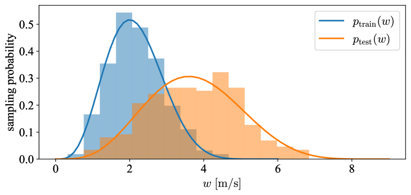
Figure 2: Training distribution $p_{\mathrm{train}}$ and test distribution $p_{\mathrm{test}}$ for the wind velocity $w$ along the inertial $x$-axis. Both are scaled beta distributions; $p_{\mathrm{train}}$ is supported on the interval $[0,6]~{}\mathrm{m/s}$ with shape parameters $(\alpha,\beta)=(5,9)$, while $p_{\mathrm{test}}$ is supported on the interval $[0,9]~{}\mathrm{m/s}$ with shape parameters $(\alpha,\beta)=(5,7)$. The normalized histograms show the distribution of the actual wind velocity samples in the training and test data for a single seed and those in the test data, and highlight the out-of-distribution samples (i.e., relative to $p_{\mathrm{train}}$) that occur during testing.

In Section 7.5, we will present test results for closed-loop tracking control simulations. In particular, we want to assess the ability of each adaptive controller to generalize to conditions different from those experienced during training data collection. To this end, during testing we always sample wind velocities from the test distribution in Figure 2, which is different from that used for the training data $\{\mathcal{T}_{j}\}_{j=1}^{M}$. In particular, the test distribution has a higher mode and larger support than the training distribution, thereby producing so-called out-of-distribution wind velocities at test time. In general, the robustness of meta-learned models and controllers to out-of-distribution tasks and train-test distribution shift is a core desideratum in meta-learning literature (Hospedales et al., 2021).

7.5 Results and Discussion

We now present empirical test results for simulations of the PFAR and PVTOL systems subject to wind gust disturbances. For both systems, we compare the trajectory tracking performance of our meta-learned adaptive controller to the baseline methods outline in Section 7.3. Our experiments are done in Python using NumPy (Harris et al., 2020) and JAX (Bradbury et al., 2018). We use the explicit nature of Pseudo-Random Number Generation (PRNG) in JAX to set a seed prior to meta-training, and then methodically branch off the associated PRNG key as required throughout the train-test experiment pipeline. Thus, all of our results can be easily reproduced; code to do so is provided at https://github.com/StanfordASL/Adaptive-Control-Oriented-Meta-Learning.

A benefit of our method is that it meta-learns model feature parameters $\varphi$, control gains (either $(\Lambda,K)$ for the PFAR system or $(c_{x},c_{y},k_{x},k_{y},k_{\phi})$ for the PVTOL system), and the adaptation gain $\Gamma$ offline. On the other hand, both the nominal feedback control and MRR baselines require gain tuning in practice by interacting with the real system. However, for the sake of comparison, we test every method with various combinations of feature parameters and control gains for each system on the same set of test trajectories.

7.5.1 Testing on PFAR

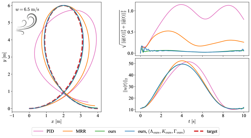
Figure 3: Tracking results for the PFAR on a “loop-the-loop” with ${w=6.5~{}\mathrm{m/s}}$, $M=10$, and $(\Lambda,K,\Gamma)=(I,10I,10I)$. We also apply our meta-learned features and gains $(\Lambda_{\mathrm{ours}},K_{\mathrm{ours}},\Gamma_{\mathrm{ours}})$. Every method expends similar control effort. However, with our meta-learned features, the tracking error ${\lVert x-x^{*}\rVert_{2}=\sqrt{\lVert\tilde{q}\rVert_{2}^{2}+\lVert\dot{\tilde{q}}\rVert_{2}^{2}}}$ (where $x$ is overloaded to denote both position $x\in\mathbb{R}$ and state $x=(q,\dot{q})$) quickly decays after a short transient, while the effect of the wind pushing the vehicle to the right is more pronounced for the baselines.

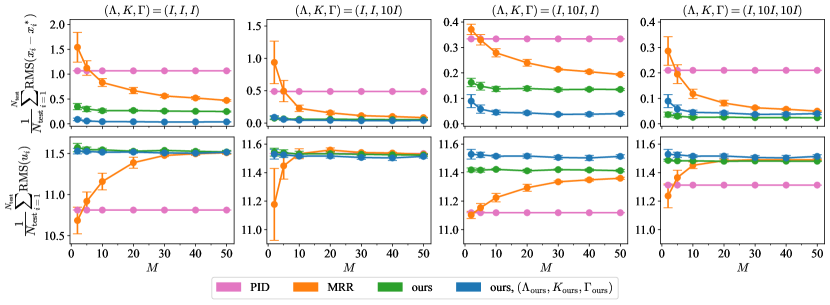
Figure 4: Line plots of the average RMS tracking error $\frac{1}{N_{\mathrm{test}}}\sum_{i=1}^{N_{\mathrm{test}}}\mathrm{RMS}(x_{i}-x^{*}_{i})$ and average control effort $\frac{1}{N_{\mathrm{test}}}\sum_{i=1}^{N_{\mathrm{test}}}\mathrm{RMS}(u_{i})$ for the PFAR system across $N_{\mathrm{test}}=200$ test trajectories versus the number of trajectories $M\in\{2,5,10,20,30,40,50\}$ in the training data. For each method, we try out various control and adaptation gains $(\Lambda,K,\Gamma)$. With our method, we also use our meta-learned gains $(\Lambda_{\mathrm{ours}},K_{\mathrm{ours}},\Gamma_{\mathrm{ours}})$. Dots and error bars denote means and standard deviations, respectively, across 10 random seeds. The results for the PID controller do not vary since it does not require any training.

For the PFAR system, we first provide a qualitative plot of tracking results for each method on a single “loop-the-loop” trajectory in Figure 3, which clearly shows that our meta-learned features induce better tracking results than the baselines, while requiring a similar expenditure of control effort. For our method, the initial transient decays quickly, thereby demonstrating fast adaptation and the potential to handle even time-varying disturbances.

For a more thorough analysis, we consider the Root-Mean-Squared (RMS) tracking error and control effort for each test trajectory $\{x^{*}_{i}\}_{i=1}^{N_{\mathrm{test}}}$; for any vector-valued signal $h(t)$ and sampling times $\{t^{(k)}\}_{k=0}^{N}$, we define

$$\mathrm{RMS}(h)\coloneqq\sqrt{\frac{1}{N}\sum_{k=0}^{N}\lVert h(t^{(k)})\rVert_{2}^{2}}.$$ (51)

We are interested in $\mathrm{RMS}(x_{i}-x^{*}_{i})$ and $\mathrm{RMS}(u_{i})$, where $x_{i}(t)=(q_{i}(t),\dot{q}_{i}(t))$ and $u_{i}(t)$ are the resultant state and control trajectories from tracking ${x^{*}_{i}(t)=(q^{*}_{i}(t),\dot{q}^{*}_{i}(t))}$. In Figure 4, we plot the averages ${\frac{1}{N_{\mathrm{test}}}\sum_{i=1}^{N_{\mathrm{test}}}\mathrm{RMS}(x_{i}-x^{*}_{i})}$ and $\frac{1}{N_{\mathrm{test}}}\sum_{i=1}^{N_{\mathrm{test}}}\mathrm{RMS}(u_{i})$ across $N_{\mathrm{test}}=200$ test trajectories for each method. For our method and the MRR baseline, we vary the number of training trajectories $M$, and thus the number of wind velocities from the training distribution in Figure 2 implicitly present in the training data. From Figure 4, we observe the PID controller usually yields the highest tracking error, thereby indicating the utility of meta-learning features $y(q,\dot{q};\varphi)$ to better compensate for $f_{\mathrm{ext}}(q,\dot{q})$. We further observe in Figure 4 that, regardless of the control gains, using our features $y(q,\dot{q};\varphi)$ in the adaptive controller 28 yields the lowest tracking error. Moreover, using our features with our meta-learned gains yields the lowest tracking error in all but one case. Our features sometimes induce a slightly higher control effort, especially when used with our meta-learned gains $(\Lambda_{\mathrm{ours}},K_{\mathrm{ours}},\Gamma_{\mathrm{ours}})$. This is most likely since the controller can better match the disturbance $f_{\mathrm{ext}}(q,\dot{q})$ with our features in closed-loop, and is an acceptable trade-off for improved tracking performance, which is our primary objective. In addition, when using our features with manually chosen or our meta-learned gains, the tracking error remains relatively constant over $M$; conversely, the tracking error for the MRR baseline is higher for lower $M$, and only reaches the performance of our method with certain gains for large $M$. Overall, our results indicate:

• The features $y(q,\dot{q};\varphi)$ meta-learned by our control-oriented method are better conditioned for closed-loop tracking control across a range of controller gains, particularly in the face of a distributional shift between training and test scenarios.

• The gains meta-learned by our method are competitive without manual tuning, and thus can be deployed immediately or serve as a good initialization for further fine-tuning.

• Our control-oriented meta-learning method is sample-efficient with respect to how much system variability is implicitly captured in the training data.

We again stress these comparisons could only be done by tuning the control gains for the baselines, which in practice would require interaction with the real system and hence further data collection. Thus, the fact that our control-oriented method can meta-learn good control gains offline is a key advantage over regression-oriented meta-learning.

7.5.2 Testing on PVTOL

Before testing and comparing our method to the baseline controller methods described in Section 7.3, we must choose controller and adaptation gains for the baseline methods. Let us collectively notate the controller gains for the nominal differential-flatness-based controller 39 as

$$\kappa\coloneqq(c_{x},c_{y},k_{x},k_{y},k_{\phi}).$$ (52)

For all tests on the PVTOL system, we compare the adaptive controller 33 with our meta-learned gains to the following baseline configurations:

1. the nominal controller with no adaptation and the initial controller gains $\kappa_{\mathrm{init}}$ used to collect training data;

2. the nominal controller with no adaptation and the meta-learned controller gains $\kappa_{\mathrm{ours}}$ from our method;

3. the adaptive controller 33 with features learned via the MRR baseline, the initial controller gains $\kappa_{\mathrm{init}}$ used to collect training data, and the adaptation gain $\Gamma_{\mathrm{init}}$ from initialization of our meta-learned parameters; and

4. the adaptive controller 33 with features learned via the MRR baseline, and the meta-learned controller and adaptation gains $(\kappa_{\mathrm{ours}},\Gamma_{\mathrm{ours}})$ from our method.

Our goal with this set of configurations is an ablation study wherein the incremental benefits from using: 1) adaptation, 2) our meta-learned gains, and 3) our meta-learned features are demonstrated.

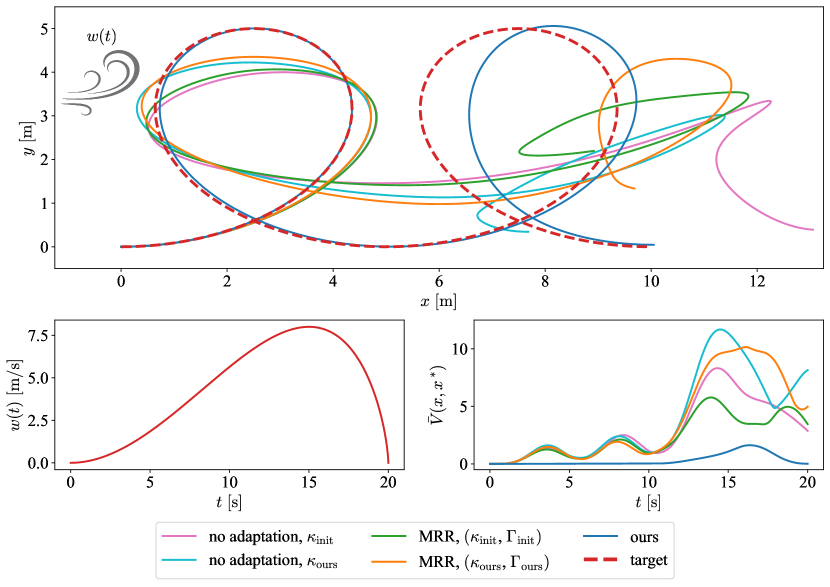
Figure 5: Tracking results for the PVTOL system on a double “loop-the-loop” with $M=10$ and a time-varying wind velocity $w(t)$. The certificate function $\bar{V}$ from 42 is also plotted to summarize the state tracking performance (where $x$ is overloaded to denote both position $x\in\mathbb{R}$ and vehicle state $x\in\mathbb{R}^{6}$). The value of $\bar{V}$ for our meta-learned adaptive controller shows a “bump” at the time when the vehicle is buffeted away from the target trajectory by the wind.

We begin by visualizing tracking results on a double “loop-the-loop” trajectory in Figure 5, with a time-varying wind velocity $w(t)$ that peaks at $8~{}\mathrm{m/s}$, which lies outside of the training distribution in Figure 2. We also plot the certificate function $\bar{V}$ from 42 as a succinct scalar summary of the tracking performance for each method. From the first loop, we see immediately that all of the controllers except ours is significantly perturbed by even a small wind disturbance. As the wind velocity increases into the second loop, the vehicle using our meta-learned adaptive controller is marginally buffeted away from the target trajectory, but recovers as it exits the loop. Meanwhile, all of the other configurations suffer greatly from the high wind during the second loop.

Figure 6: Line plots of the average RMS tracking error $\frac{1}{N_{\mathrm{test}}}\sum_{i=1}^{N_{\mathrm{test}}}\mathrm{RMS}(x_{i}-x^{*}_{i})$ for the PVTOL system over ${N_{\mathrm{test}}=200}$ test trajectories versus the number of trajectories ${M\in\{2,5,10,20,30,40,50\}}$ in the training data. The results for the nominal feedback controller without any learned components do not vary since it does not require any training. Dots and error bars denote means and standard deviations, respectively, across 10 random seeds.

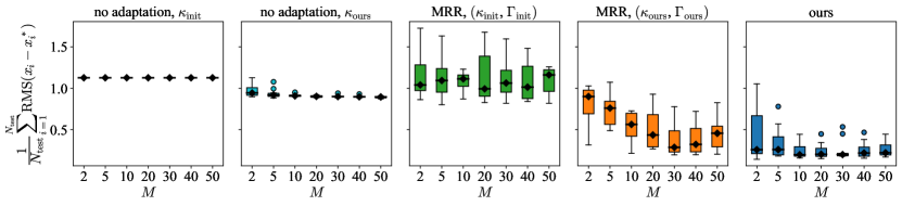
Figure 7: Tukey box-and-whisker plots of the average RMS tracking error $\frac{1}{N_{\mathrm{test}}}\sum_{i=1}^{N_{\mathrm{test}}}\mathrm{RMS}(x_{i}-x^{*}_{i})$ for the PVTOL system over $N_{\mathrm{test}}=200$ test trajectories versus the number of trajectories $M\in\{2,5,10,20,30,40,50\}$ in the training data, for each controller configuration. The box plot statistics are computed across 10 random seeds. Medians are marked by black diamonds. The 25-th and 75-th percentiles are marked by the bottom and top edges, respectively, of each box. Each whisker extends an additional 1.5 times the interquartile range beyond the box edge. Outliers are marked by circles. The results for the nominal feedback controller without any learned components do not vary since it does not require any training.

In a similar fashion to what we did for the PFAR system, we also analyze the average RMS tracking error ${\frac{1}{N_{\mathrm{test}}}\sum_{i=1}^{N_{\mathrm{test}}}\mathrm{RMS}(x_{i}-x^{*}_{i})}$ for each method across $200$ test trajectories, each alongside a fixed wind velocity $w$ sampled from the test distribution in Figure 2. For each configuration, we once again vary the number of training trajectories $M$, and thus the number of wind velocities from the training distribution in Figure 2 implicitly present in the training data. Figure 6 depicts the mean and standard deviation of ${\frac{1}{N_{\mathrm{test}}}\sum_{i=1}^{N_{\mathrm{test}}}\mathrm{RMS}(x_{i}-x^{*}_{i})}$ across 10 random seeds for each configuration. Figure 7 displays more detail in the form of box plots for the average RMS tracking error across these seeds for each configuration. The spread in each plot is due to the effect the random seed has on sampling $M$ trajectories, initializing parameters, and stochastic batch gradient descent during meta-training in our method and the MRR baseline. From Figure 6 and Figure 7, beyond noting that our meta-learned adaptive controller outperforms all of the baselines, we make the following observations:

• In comparing the non-adaptive controllers with $\kappa_{\mathrm{init}}$ and $\kappa_{\mathrm{ours}}$, we see that our meta-learned control gains are an improvement over $\kappa_{\mathrm{init}}$.

• In comparing the non-adaptive controllers to the adaptive controller using features meta-learned with MRR and $(\kappa_{\mathrm{init}},\Gamma_{\mathrm{init}})$, we see that MRR can learn features that lead to poor closed-loop performance without gain tuning.

• In comparing the adaptive controller using features meta-learned with MRR and $(\kappa_{\mathrm{ours}},\Gamma_{\mathrm{ours}})$ to the other baseline configurations, we see that adaptation can lead to improved tracking performance with gain tuning.

• Finally, in comparing our meta-learned adaptive controller to the adaptive controller using features meta-learned with MRR and $(\kappa_{\mathrm{ours}},\Gamma_{\mathrm{ours}})$, we see once again that our meta-learned features are better conditioned for closed-loop tracking control.

Overall, adaptation, tuned control and adaptation gains, and parametric model features individually have the potential to incrementally improve closed-loop performance. Critically, our meta-learning framework trains these components in an end-to-end fashion to realize the sum of these improvements.

8 Conclusions & Future Work

In this work, we formalized control-oriented meta-learning of adaptive controllers for nonlinear dynamical systems, offline from trajectory data. The procedure we presented is general and uses adaptive control as the base-learner to attune learning to the downstream control objective. We then specialized our procedure to fully-actuated Lagrangian and general control-affine dynamical systems, with adaptive controller designs parameterized by control gains, an adaptation gain, and nonlinear model features. We demonstrated that our control-oriented meta-learning method engenders better closed-loop tracking control performance at test time than when learning is done for the purpose of model regression.

There are a number of exciting future directions for this work. In particular, we are interested in control-oriented meta-learning with constraints, such as for adaptive Model Predictive Control (MPC) (Adetola and Guay, 2011; Bujarbaruah et al., 2018; Soloperto et al., 2019; Köhler et al., 2020; Sinha et al., 2022) with state and input constraints. Back-propagating through such a controller would leverage recent work on differentiable convex optimization (Amos et al., 2018; Agrawal et al., 2019, 2020). We could also back-propagate through parameter constraints; for example, physical consistency of adapted inertial parameters can be enforced as Linear Matrix Inequality (LMI) constraints that reduce overfitting and improve parameter convergence (Wensing et al., 2017).

In addition, we want to extend our meta-learning framework in a principled manner to adaptive control for systems with unmatched uncertainties. Such uncertainties present a fundamental challenge for traditional adaptive controllers, since they cannot be cancelled stably by the control input (Lopez and Slotine, 2020; Sinha et al., 2022). Lopez and Slotine (2022) established a universal adaptation law using stability certificate functions, such as Lyapunov functions and Control Contraction Metrics (CCMs) (Manchester and Slotine, 2017), that are parameterized as a family of certificate functions corresponding to all possible values of the unmatched uncertainty, rather than just using a single certificate function corresponding to the nominal dynamics. To this end, we want to explore how meta-learning can be used to train such universal adaptive controllers defined in part by parametric stability certificates. This could build off of existing work on learning such certificates from data (Richards et al., 2018; Singh et al., 2020; Boffi et al., 2020; Tsukamoto et al., 2021).

We thank Masha Itkina for her invaluable feedback, and Matteo Zallio for his expertise in crafting Figure 1.

This research was supported in part by the National Science Foundation (NSF) via Cyber-Physical Systems (CPS) award #1931815 and Energy, Power, Control, and Networks (EPCN) award #1809314, and the National Aeronautics and Space Administration (NASA) University Leadership Initiative via grant #80NSSC20M0163. Spencer M. Richards was also supported in part by the Natural Sciences and Engineering Research Council of Canada (NSERC). This article solely reflects the authors’ own opinions and conclusions, and not those of any NSF, NASA, or NSERC entity.

The authors declare that there is no conflict of interest.

Appendix A Training Details

A.1 Our Method

Before meta-training, for both the PFAR and PVTOL systems we first train an ensemble of $M$ models $\{\hat{f}_{j}\}_{j=1}^{M}$, one for each trajectory $\mathcal{T}_{j}$, via gradient descent on the regression objective 12 with $\mu_{\mathrm{ensem}}=10^{-4}$ and a single fourth-order Runge-Kutta step to approximate the integral over $t^{(k+1)}_{j}-t^{(k)}_{j}=0.01~{}\mathrm{s}$. We set each $\hat{f}_{j}$ as a feed-forward neural network with $2$ hidden layers, each containing $32$ $\tanh(\cdot)$ neurons. We perform a random $75\%/25\%$ split of the transition tuples in $\mathcal{T}_{j}$ into a training set $\mathcal{T}_{j}^{\mathrm{train}}$ and validation set $\mathcal{T}_{j}^{\mathrm{valid}}$, respectively. We do batch gradient descent via Adam [Kingma and Ba, 2015] on $\mathcal{T}_{j}^{\mathrm{train}}$ with a step size of $10^{-2}$, over $1000$ epochs with a batch size of $\lfloor 0.25|\mathcal{D}_{j}^{\mathrm{train}}|\rfloor$, while recording the regression loss with $\mu_{\mathrm{ensem}}=0$ on $\mathcal{T}_{j}^{\mathrm{valid}}$. We proceed with the parameters for $\hat{f}_{j}$ corresponding to the lowest recorded validation loss.

With the trained ensemble $\{\hat{f}_{j}\}_{j=1}^{M}$, we can now meta-train $\theta_{\mathrm{ours}}\coloneqq(\varphi,\Lambda,K,\Gamma)$ for the PFAR system or $\theta_{\mathrm{ours}}=(\varphi,c_{x},c_{y},k_{x},k_{y},k_{\phi},\Gamma)$ for the PVTOL system. First, we randomly generate ${N=10}$ smooth target trajectories $\{x^{*}_{i}\}_{i=1}^{N}$ in the same manner described in Section 7.2. We then randomly sub-sample ${N_{\mathrm{train}}=\lfloor 0.75N\rfloor=7}$ target trajectories and $M_{\mathrm{train}}=\lfloor 0.75M\rfloor$ models from the ensemble to form the meta-training set $\{(x^{*}_{i},\hat{f}_{j})\}_{i=1,j=1}^{N_{\mathrm{train}},M_{\mathrm{train}}}$, while the remaining models and target trajectories form the meta-validation set. We set $\hat{A}y(x;\varphi)$ as a feed-forward neural network with $2$ hidden layers of $32$ $\tanh(\cdot)$ neurons each, where the adapted parameters $\hat{A}(t)\in\mathbb{R}^{d\times 32}$ serve as the output layer. We set up the meta-problem 11 using $\{(x^{*}_{i},\hat{f}_{j})\}_{i=1,j=1}^{N_{\mathrm{train}},M_{\mathrm{train}}}$, $\mu_{\mathrm{ctrl}}=10^{-3}$, $\mu_{\mathrm{meta}}=10^{-4}$, and either the adaptive controller 28 for the PFAR system or the adaptive controller 33 for the PVTOL system. We then perform gradient descent via Adam with a step size of $10^{-2}$ to train $\theta_{\mathrm{ours}}$. We compute the integral in 11 via a fourth-order Runge-Kutta integration scheme with a fixed time step of $0.01~{}\mathrm{s}$. We back-propagate gradients through this computation in a manner similar to Zhuang et al. [2020], rather than using the adjoint method for neural ODEs [Chen et al., 2018], due to our observation that the backward pass is sensitive to any numerical error accumulated along the forward pass during closed-loop control simulations. We perform $500$ gradient steps while recording the meta-loss from 11 with $\mu_{\mathrm{meta}}=0$ on the meta-validation set, and take the best meta-parameters $\theta_{\mathrm{ours}}$ as those corresponding to the lowest recorded validation loss.

A.2 MRR Baseline

To meta-train $\theta_{\mathrm{MRR}}\coloneqq\varphi$, we first perform a random $75\%/25\%$ split of the transition tuples in each trajectory $\mathcal{T}_{j}$ to form a meta-training set $\{\mathcal{T}_{j}^{\mathrm{meta\text{-}train}}\}_{j=1}^{M}$ and a meta-validation set $\{\mathcal{T}_{j}^{\mathrm{meta\text{-}valid}}\}_{j=1}^{M}$. We set $\hat{A}y(x;\varphi)$ as a feed-forward neural network with $2$ hidden layers of $32$ $\tanh(\cdot)$ neurons each, where the adapted parameters $\hat{A}(t)\in\mathbb{R}^{d\times 32}$ serve as the output layer. We construct the meta-problem 4 using the task loss 50, the adaptation mechanism 49, and $\mu_{\mathrm{meta}}=10^{-4}$; for this, we use transition tuples from $\mathcal{T}_{j}^{\mathrm{meta\text{-}train}}$. We then meta-train $\theta_{\mathrm{MRR}}$ via gradient descent using Adam with a step-size of $10^{-2}$ for $5000$ steps; at each step, we randomly sample a subset of $\lfloor 0.25|\mathcal{T}_{j}^{\mathrm{meta\text{-}train}}|\rfloor$ tuples from $\mathcal{T}_{j}^{\mathrm{meta\text{-}train}}$ to use in the closed-form ridge regression solution. We also record the meta-loss with $\mu_{\mathrm{meta}}=0$ on the meta-validation set at each step, and take the best meta-parameters $\theta_{\mathrm{MRR}}$ as those corresponding to the lowest recorded validation loss.

References

- Adetola and Guay [2011] V. Adetola and M. Guay. Robust adaptive MPC for constrained uncertain nonlinear systems. Int. Journal of Adaptive Control and Signal Processing, 25(2):155–167, 2011.
- Agrawal et al. [2019] A. Agrawal, S. Barratt, S. Boyd, E. Busseti, and W. M. Moursi. Differentiating through a conic program. Journal of Applied and Numerical Optimization, 1(2):107–115, 2019.
- Agrawal et al. [2020] A. Agrawal, S. Barratt, S. Boyd, and B. Stellato. Learning convex optimization control policies. In Learning for Dynamics & Control, 2020.
- Ailon [2010] A. Ailon. Simple tracking controllers for autonomous VTOL aircraft with bounded inputs. IEEE Transactions on Automatic Control, 55(3):737–743, 2010.
- Amos et al. [2018] B. Amos, I. D. J. Rodriguez, J. Sacks, B. Boots, and J. Z. Kolter. Differentiable MPC for end-to-end planning and control. In Conf. on Neural Information Processing Systems, 2018.
- Anderson and Johnson [1982] B. D. O. Anderson and C. R. Johnson, Jr. Exponential convergence of adaptive identification and control algorithms. Automatica, 18(1):1–13, 1982.
- Andersson et al. [2019] J. A. E. Andersson, J. Gillis, G. Horn, J. B. Rawlings, and M. Diehl. CasADi: A software framework for nonlinear optimization and optimal control. Mathematical Programming Computation, 11(1):1–36, 2019.
- Angeli [2002] D. Angeli. A Lyapunov approach to incremental stability properties. IEEE Transactions on Automatic Control, 47(3):410–422, 2002.
- Aseltine et al. [1958] J. Aseltine, A. Mancini, and C. Sarture. A survey of adaptive control systems. IRE Transactions on Automatic Control, 6(1):102–108, 1958.
- Azizan and Hassibi [2019] N. Azizan and B. Hassibi. Stochastic gradient/mirror descent: Minimax optimality and implicit regularization. In Int. Conf. on Learning Representations, 2019.
- Azizan et al. [2021] N. Azizan, S. Lale, and B. Hassibi. Stochastic mirror descent on overparameterized nonlinear models. IEEE Transactions on Neural Networks and Learning Systems, 2021. Early access.
- Barbălat [1959] I. Barbălat. Systèmes d’équations différentielles d’oscillations non linéaires (Systems of differential equations of nonlinear oscillations). Revue Roumaine de Mathématiques Pures et Appliquées, 4:267–270, 1959.
- Belkhale et al. [2021] S. Belkhale, R. Li, G. Kahn, R. McAllister, R. Calandra, and S. Levine. Model-based meta-reinforcement learning for flight with suspended payloads. IEEE Robotics and Automation Letters, 2021. In press.
- Bertinetto et al. [2019] L. Bertinetto, J. Henriques, P. H. S. Torr, and A. Vedaldi. Meta-learning with differentiable closed-form solvers. In Int. Conf. on Learning Representations, 2019.
- Boffi and Slotine [2021] N. M. Boffi and J.-J. E. Slotine. Implicit regularization and momentum algorithms in nonlinearly parameterized adaptive control and prediction. Neural Computation, 33(3):590–673, 2021.
- Boffi et al. [2020] N. M. Boffi, S. Tu, N. Matni, J.-J. E. Slotine, and V. Sindhwani. Learning stability certificates from data. In Conf. on Robot Learning, 2020.
- Boffi et al. [2021] N. M. Boffi, S. Tu, and J.-J. Slotine. Nonparametric adaptive control and prediction: Theory and randomized algorithms. In Proc. IEEE Conf. on Decision and Control, 2021.
- Boyd and Sastry [1986] S. Boyd and S. S. Sastry. Necessary and sufficient conditions for parameter convergence in adaptive control. Automatica, 22(6):629–639, 1986.
- Bradbury et al. [2018] J. Bradbury, R. Frostig, P. Hawkins, M. J. Johnson, C. Leary, D. Maclaurin, G. Necula, A. Paszke, J. VanderPlas, S. Wanderman-Milne, and Q. Zhang. JAX: Composable transformations of Python+NumPy programs, 2018. Available at http://github.com/google/jax.
- Brescianini and D’Andrea [2018] D. Brescianini and R. D’Andrea. Computationally efficient trajectory generation for fully actuated multirotor vehicles. IEEE Transactions on Robotics, 34(3):555–571, 2018.
- Bujarbaruah et al. [2018] M. Bujarbaruah, X. Zhang, U. Rosolia, and R. Borrelli. Adaptive MPC for iterative tasks. In Proc. IEEE Conf. on Decision and Control, 2018.
- Chang et al. [2019] Y.-C. Chang, N. Roohi, and S. Gao. Neural Lyapunov control. In Conf. on Neural Information Processing Systems, 2019.
- Chen et al. [2018] R. T. Q. Chen, Y. Rubanova, J. Bettencourt, and D. Duvenaud. Neural ordinary differential equations. In Conf. on Neural Information Processing Systems, 2018.
- Clavera et al. [2018] I. Clavera, J. Rothfuss, J. Schulman, Y. Fujita, T. Asfour, and P. Abbeel. Model-based reinforcement learning via meta-policy optimization. In Conf. on Robot Learning, 2018.
- Finn et al. [2017] C. Finn, P. Abbeel, and S. Levine. Model-agnostic meta-learning for fast adaptation of deep networks. In Int. Conf. on Machine Learning, 2017.
- Forssell and Ljung [2000] U. Forssell and L. Ljung. Some results on optimal experiment design. Automatica, 36(5):749–756, 2000.
- Gahlawat et al. [2020] A. Gahlawat, P. Zhao, A. Patterson, N. Hovakimyan, and E. A. Theodorou. -: adaptive control with Bayesian learning. In Learning for Dynamics & Control, 2020.
- Gevers [2005] M. Gevers. Identification for control: From the early achievements to the revival of experiment design. European Journal of Control, 11(4–5):335–352, 2005.
- Grande et al. [2013] R. C. Grande, G. Chowdhary, and J. P. How. Nonparametric adaptive control using Gaussian processes with online hyperparameter estimation. In Proc. IEEE Conf. on Decision and Control, 2013.
- Harris et al. [2020] C. R. Harris, K. J. Millman, S. J. Van der Walt, R. Gommers, P. Virtanen, D. Cournapeau, E. Wieser, J. Taylor, S. Berg, N. J. Smith, R. Kern, M. Picus, S. Hoyer, M. H. Van Kerkwijk, M. Brett, A. Haldane, J. F. Del Río, M. Wiebe, P Peterson, P. Gérard-Marchant, K. Sheppard, T. Reddy, W. Weckesser, H. Abbasi, C. Gohlke, and T. E. Oliphant. Array programming with NumPy. Nature, 585(7825):357–362, 2020.
- Harrison et al. [2018a] J. Harrison, A. Sharma, R. Calandra, and M. Pavone. Control adaptation via meta-learning dynamics. In Conf. on Neural Information Processing Systems - Workshop on Meta-Learning, 2018a.
- Harrison et al. [2018b] J. Harrison, A. Sharma, and M. Pavone. Meta-learning priors for efficient online bayesian regression. In Workshop on Algorithmic Foundations of Robotics, 2018b.
- Hauser et al. [1992] J. Hauser, S. Sastry, and G. Meyer. Nonlinear control design for slightly non-minimum phase systems: Application to V/STOL aircraft. Automatica, 28(4):665–679, 1992.
- Hjalmarsson et al. [1996] H. Hjalmarsson, M. Gevers, and F. de Bruyne. For model-based control design, closed-loop identification gives better performance. Automatica, 32(12):1659–1673, 1996.
- Hospedales et al. [2021] T. M. Hospedales, A. Antoniou, P. Micaelli, and A. J. Storkey. Meta-learning in neural networks: A survey. IEEE Transactions on Pattern Analysis & Machine Intelligence, 2021. Early access.
- Ioannou and Sun [2012] P. Ioannou and J. Sun. Robust Adaptive Control. Dover Publications, 2012.
- Joshi and Chowdhary [2019] G. Joshi and G. Chowdhary. Deep model reference adaptive control. In Proc. IEEE Conf. on Decision and Control, 2019.
- Joshi et al. [2020] G. Joshi, J. Virdi, and G. Chowdhary. Asynchronous deep model reference adaptive control. In Conf. on Robot Learning, 2020.
- Kamel et al. [2018] M. Kamel, S. Verling, O. Elkhatib, C. Sprecher, P. Wulkop, Z. Taylor, R. Siegwart, and I. Gilitschenski. The Voliro omniorientational hexacopter: An agile and maneuverable tiltable-rotor aerial vehicle. IEEE Robotics and Automation Magazine, 25(4):34–44, 2018.
- Khalil [2002] H. K. Khalil. Nonlinear Systems. Prentice Hall, third edition, 2002.
- Khansari-Zadeh and Billard [2011] S. M. Khansari-Zadeh and A. Billard. Learning stable nonlinear dynamical systems with Gaussian mixture models. IEEE Transactions on Robotics, 27(5):943–957, 2011.
- Kingma and Ba [2015] D. P. Kingma and J. L. Ba. Adam: A method for stochastic optimization. In Int. Conf. on Learning Representations, 2015.
- Köhler et al. [2020] J. Köhler, P. Kötting, R. Soloperto, F. Allgöwer, and M. A. Müller. A robust adaptive model predictive control framework for nonlinear uncertain systems. Int. Journal of Robust and Nonlinear Control, 2020. In press.
- Kurutach et al. [2018] T. Kurutach, I. Clavera, Y. Duan, A. Tamar, and P. Abbeel. Model-ensemble trust-region policy optimization. In Int. Conf. on Learning Representations, 2018.
- Lakshminarayanan et al. [2017] B. Lakshminarayanan, A. Pritzel, and C. Blundell. Simple and scalable predictive uncertainty estimation using deep ensembles. In Conf. on Neural Information Processing Systems, 2017.
- Landau et al. [2011] I. D. Landau, R. Lozano, M. M’Saad, and A. Karimi. Adaptive Control: Algorithms, Analysis and Applications. Springer-Verlag, 2 edition, 2011.
- LaSalle [1960] J. P. LaSalle. Some extensions of Liapunov’s second method. IRE Transactions on Circuit Theory, 7(4):520–527, 1960.
- Lee et al. [2019] K. Lee, S. Maji, A. Ravichandran, and S. Soatto. Meta-learning with differentiable convex optimization. In IEEE Conf. on Computer Vision and Pattern Recognition, 2019.
- Ljung [1999] L. Ljung. System Identification: Theory for the User. Prentice Hall PTR, 2 edition, 1999.
- Lohmiller and Slotine [1998] W. Lohmiller and J.-J. E. Slotine. On contraction analysis for non-linear systems. Automatica, 34(6):683–696, 1998.
- Lopez and Slotine [2020] B. T. Lopez and J.-J. E. Slotine. Adaptive nonlinear control with contraction metrics. IEEE Control Systems Letters, 5(1):205–210, 2020.
- Lopez and Slotine [2022] B. T. Lopez and J.-J. E. Slotine. Universal adaptive control of nonlinear systems. IEEE Control Systems Letters, 6(1):1826–1830, 2022.
- Lyapunov [1892] A. M. Lyapunov. Obshchaya zadacha ob ustoichivosti dvizheniya (The General Problem of the Stability of Motion). PhD thesis, Kharkov Mathematical Society, 1892.
- Manchester and Slotine [2017] I. R. Manchester and J.-J. E. Slotine. Control contraction metrics: Convex and intrinsic criteria for nonlinear feedback design. IEEE Transactions on Automatic Control, 62(6):3046–3053, 2017.
- Mareels et al. [1987] I. M. Y. Mareels, B. D. O. Anderson, R. R. Bitmead, M. Bodson, and S. S. Sastry. Revisiting the MIT rule for adaptive control. In IFAC Workshop on Adaptive Systems in Control and Signal Processing, 1987.
- Medina and Billard [2017] J. R. Medina and A. Billard. Learning stable task sequences from demonstration with linear parameter varying systems and hidden Markov models. In Conf. on Robot Learning, 2017.
- Mellinger and Kumar [2011] D. Mellinger and V. Kumar. Minimum snap trajectory generation and control for quadrotors. In Proc. IEEE Conf. on Robotics and Automation, 2011.
- Millard et al. [2020] D. Millard, E. Heiden, S. Agrawal, and G. S. Sukhatme. Automatic differentiation and continuous sensitivity analysis of rigid body dynamics. Available at https://arxiv.org/abs/2001.08539, 2020.
- Nagabandi et al. [2019] A. Nagabandi, I. Clavera, S. Liu, R. S. Fearing, P. Abbeel, S. Levine, and C. Finn. Learning to adapt in dynamic, real-world environments through meta-reinforcement learning. In Int. Conf. on Learning Representations, 2019.
- Narendra and Annaswamy [2005] K. S. Narendra and A. M. Annaswamy. Stable Adaptive Systems. Dover Publications, 2005.
- Narendra and Valavani [1978] K. S. Narendra and L. S. Valavani. Stable adaptive controller design – direct control. IEEE Transactions on Automatic Control, 23(4):570–583, 1978.
- Narendra et al. [1980] K. S. Narendra, Y.-H. Lin, and L. S. Valavani. Stable adaptive controller design, part II: Proof of stability. IEEE Transactions on Automatic Control, 25(3):440–448, 1980.
- Niemeyer and Slotine [1991] G. Niemeyer and J.-J. E. Slotine. Performance in adaptive manipulator control. Int. Journal of Robotics Research, 10(2):149–161, 1991.
- O’Connell et al. [2021] M. O’Connell, G. Shi, X. Shi, and S.-J. Chung. Meta-learning-based robust adaptive flight control under uncertain wind conditions. Available at https://arxiv.org/abs/2103.01932, 2021.
- Pinheiro and Bates [1996] J. C. Pinheiro and D. M. Bates. Unconstrained parametrizations for variance-covariance matrices. Statistics and Computing, 6(3):289–296, 1996.
- Pontryagin et al. [1962] L. S. Pontryagin, V. G. Boltyanskii, R. V. Gamkrelidze, and E. F. Mishchenko. The Mathematical Theory of Optimal Processes. Wiley Interscience, 1962.
- Rajeswaran et al. [2017] A. Rajeswaran, S. Ghotra, B. Ravindran, and S. Levine. EPOpt: Learning robust neural network policies using model ensembles. In Int. Conf. on Learning Representations, 2017.
- Rajeswaran et al. [2019] A. Rajeswaran, C. Finn, S. Kakade, and S. Levine. Meta-learning with implicit gradients. In Conf. on Neural Information Processing Systems, 2019.
- Rashad et al. [2020] R. Rashad, J. Goerres, R. Aarts, J. B. C. Engelen, and S. Stramigioli. Fully actuated multirotor UAVs. IEEE Robotics and Automation Magazine, 27(3):97–107, 2020.
- Åström and Murray [2020] K. J. Åström and R. M. Murray. Feedback Systems: An Introduction for Scientists and Engineers. Princeton Univ. Press, 2 edition, 2020. Electronic version v3.1.5.
- Åström and Wittenmark [1971] K. J. Åström and B. Wittenmark. Problems of identification and control. Journal of Mathematical Analysis and Applications, 34(1):90–113, 1971.
- Richards et al. [2018] S. M. Richards, F. Berkenkamp, and A. Krause. The Lyapunov neural network: Adaptive stability certification for safe learning of dynamical systems. In Conf. on Robot Learning, 2018.
- Richards et al. [2021] S. M. Richards, N. Azizan, J.-J. E. Slotine, and M. Pavone. Adaptive-control-oriented meta-learning for nonlinear systems. In Robotics: Science and Systems, 2021.
- Richter et al. [2013] C. Richter, A. Bry, and N. Roy. Polynomial trajectory planning for aggressive quadrotor flight in dense indoor environments. In Int. Symp. on Robotics Research, 2013.
- Ryll et al. [2017] M. Ryll, G. Muscio, F. Pierri, E. Cataldi, G. Antonelli, F. Caccavale, and A. Franchi. 6D physical interaction with a fully actuated aerial robot. In Proc. IEEE Conf. on Robotics and Automation, 2017.
- Sanner and Slotine [1992] R. M. Sanner and J.-J. E. Slotine. Gaussian networks for direct adaptive control. IEEE Transactions on Neural Networks, 3(6):837–863, 1992.
- Sanner and Slotine [1995] R. M. Sanner and J.-J. E. Slotine. Stable adaptive control of robot manipulators using “neural” networks. Neural Computation, 7(4):753–790, 1995.
- Singh et al. [2020] S. Singh, S. M. Richards, V. Sindhwani, J-J. E. Slotine, and M. Pavone. Learning stabilizable nonlinear dynamics with contraction-based regularization. Int. Journal of Robotics Research, 2020.
- Sinha et al. [2022] R. Sinha, J. Harrison, S. M. Richards, and M. Pavone. Adaptive robust model predictive control with matched and unmatched uncertainty. In American Control Conference, 2022.
- Skelton [1989] R. E. Skelton. Model error concepts in control design. Int. Journal of Control, 49(5):1725–1753, 1989.
- Slotine and Li [1987] J.-J. E. Slotine and W. Li. On the adaptive control of robot manipulators. Int. Journal of Robotics Research, 6(3):49–59, 1987.
- Slotine and Li [1989] J.-J. E. Slotine and W. Li. Composite adaptive control of robot manipulators. Automatica, 25(4):509–519, 1989.
- Slotine and Li [1991] J.-J. E. Slotine and W. Li. Applied Nonlinear Control. Prentice Hall, 1991.
- Soloperto et al. [2019] R. Soloperto, J. Köhler, M. A. Müller, and F. Allgöwer. Dual adaptive MPC for output tracking of linear systems. In Proc. IEEE Conf. on Decision and Control, 2019.
- Sun et al. [2020] D. Sun, S. Jha, and C. Fan. Learning certified control using contraction metric. In Conf. on Robot Learning, 2020.
- Tsukamoto et al. [2021] H. Tsukamoto, S.-J. Chung, and J.-J. E. Slotine. Neural stochastic contraction metrics for learning-based control and estimation. IEEE Control Systems Letters, 5(5):1825–1830, 2021.
- Wensing and Slotine [2020] P. M. Wensing and J.-J. Slotine. Beyond convexity–contraction and global convergence of gradient descent. PLoS ONE, 15(12), 2020.
- Wensing et al. [2017] P. M. Wensing, S. Kim, and J.-J. E. Slotine. Linear matrix inequalities for physically consistent inertial parameter identification: A statistical perspective on the mass distribution. IEEE Robotics and Automation Letters, 3(1):60–67, 2017.
- Zheng et al. [2020] P. Zheng, X. Tan, B. B. Kocer, E. Yang, and M. Kovac. TiltDrone: A fully-actuated tilting quadrotor platform. IEEE Robotics and Automation Letters, 5(4):6845–6852, 2020.
- Zhuang et al. [2020] J. Zhuang, N. Dvornek, X. Li, S. Tatikonda, X. Papademetris, and J. Duncan. Adaptive checkpoint adjoint method for gradient estimation in neural ODE. In Int. Conf. on Machine Learning, 2020.