Flavour anomalies and dark matter assisted unification in $SO(10)$ GUT

Abstract

With the recent experimental hint of new physics from flavor physics anomalies, combined with the evidence from neutrino masses and dark matter, we consider a minimal extension of SM with a scalar leptoquark and a fermion triplet. The scalar leptoquark with couplings to leptons and quarks can explain lepton flavor non-universality observables $R_{K}$, $R_{K^{(*)}}$, $R_{D^{(*)}}$ and $R_{J/\psi}$. Neutral component of fermion triplet provides current abundance of dark matter in the Universe. The interesting feature of the proposal is that the minimal addition of these phenomenologically rich particles (scalar leptoquark and fermion triplet) assist in realizing the unification of the gauge couplings associated with the strong and electroweak forces of standard model when embedded in the non-supersymmetric $SO(10)$ grand unified theory. We discuss on unification mass scale and the corresponding proton decay constraints while taking into account the GUT threshold corrections.

I Introduction

Standard model of particle physics (SM) beautifully explains the gauge theory of strong, electromagnetic and weak interactions, with all its predictions testified at current experiments including LHC. Still it is known that many observed phenomena like neutrino masses and mixing Bilenky (1999); Mohapatra and Senjanovic (1980); Schechter and Valle (1980); Babu and Mohapatra (1993); Hosaka et al. (2006); Ahmad et al. (2002); Abe et al. (2016, 2019); An et al. (2012); Abe et al. (2012), dark matter Zwicky (1937, 1933); Bertone et al. (2005); Mambrini et al. (2015), matter anti-matter asymmetry Sakharov (1991); Kolb and Wolfram (1980); Fukugita and Yanagida (1986); Fritzsch and Minkowski (1975) and the recent flavor anomalies, see for example Bifani et al. (2019) and references therein, cannot be addressed within its framework. This motivates to explore other possible beyond standard model (BSM) frameworks which have the potential to address these unsolved issues of the SM. It is believed that the ultimate theory of elementary particles might be an effective low energy approximation of some grand unified theory (GUT) or part of another theory at high scale.

Though most of the flavor observables go along with the SM, there are a collection of recent measurements in semileptonic $B$ meson decays, involving $b\to s\ell\ell$ ($\ell=e,\mu)$ and $b\to cl\bar{\nu}_{l}$ $(l=\mu,\tau)$ quark level transitions, that are incongruous with the SM predictions. The most conspicuous measurements, hinting the physics beyond SM are the lepton flavor universality violating parametes: $R_{K}$ with a discrepancy of $3.1\sigma$ Aaij et al. (2014a, 2019a, 2021); Bobeth et al. (2007); Bordone et al. (2016), $R_{K^{(*)}}$ with a disagreement at the level of $(2.1-2.5)\sigma$ Aaij et al. (2017); Capdevila et al. (2018), $R_{D^{(*)}}$ with $3.08\sigma$ discrepancy Amhis et al. (2021); Na et al. (2015); Fajfer et al. (2012a, b) and $R_{J/\psi}$ with a deviation of nearly $2\sigma$ Aaij et al. (2018a); Wang et al. (2013); Ivanov et al. (2005) from their SM predictions. Though the Belle Collaboration Abdesselam et al. (2021); Abdesselam et al. (2019a) has also announced their measurements on $R_{K^{(*)}}$ in various $q^{2}$ bins, however these measurements have large uncertainties. Besides the $R_{K^{(*)}}$ parameters, the $P_{5}^{\prime}$ optimized observable disagrees with the SM at the level of $4\sigma$ in the $(4.3-8.68)~{}\rm{GeV}^{2}$ $q^{2}$-bin Aaij et al. (2013a, 2016); Abdesselam et al. (2016a) and the decay rate of $B\to K^{*}\mu\mu$ shows $3\sigma$ discrepancy Aaij et al. (2014b). The branching ratio of $B_{s}\to\phi\mu\mu$ channel also disagrees with the theory at the level of $3\sigma$ Aaij et al. (2013b) in low $q^{2}$.

One of the possible explanation for these flavor anomalies is the existence of leptoquarks (LQ) leading to the transitions $b\to s\ell\ell$ and $b\to cl\bar{\nu}_{l}$. It is believed that LQs may lead to interesting new physics searches and could be the next big discovery at LHC. Since, by definition, LQ connecting both leptons and quarks simultaneously may have its origin from quark-lepton symmetry, Pati-Salam symmetry, $SO(10)$ and other grand unified models (GUT). in the present work, we wish to study LQ assisted gauge coupling unification of the fundamental forces described by the SM. In the present work, the idea is to construct a TeV scale extension of SM in order to explain the experimental hints of new physics in recently observed flavor anomalies within the framework of non-supersymmetric $SO(10)$ grand unified theory while simultaneous addressing neutrino mass and dark matter. The important feature of the model is that inclusion of a scalar LQ and a fermion triplet DM at few TeV scale on top of SM leads to successful unification of SM gauge couplings.

In the context of GUT, the popular models are $SU(5)$ Georgi and Glashow (1974), $SO(10)$ Pati and Salam (1974); Fritzsch and Minkowski (1975); Lavoura and Wolfenstein (1993); Senjanović and Mohapatra (1975); Clark et al. (1982); Altarelli and Meloni (2013a); Dueck and Rodejohann (2013a); Meloni et al. (2014, 2017); Preda et al. (2022); Chakrabortty et al. (2018); Bandyopadhyay and Raychaudhuri (2017) and $E_{6}$Gursey et al. (1976); Shafi (1978); Nandi and Sarkar (1986); Stech and Tavartkiladze (2004); Huang (2014); Dash et al. (2021a, 2020, b); Bandyopadhyay and Maji (2019), where many of the unsolved issues of the SM can be addressed. In most of the literature, it is found that all GUTs without any intermediate symmetry breaking and in the absence of supersymmetry, fails to unify the gauge couplings corresponding to three fundamental forces as described by SM. Few attempts were successful in gauge coupling unification by adding extra particles on top of SM spectrum at a higher scale. With this idea, we explore a simplified extension of SM at few TeV scale, which can be successfully embedded in a non-supersymmetric $SO(10)$ GUT. The key feature of the work is that the extra particles, isospin triplet fermion and scalar leptoquark (SLQ) which are originally motivated to unify the gauge couplings, can simultaneously address the dark matter of the Universe and flavor anomalies. While examining the gauge coupling unification it is observed that the unification scale and inverse fine structure constant are in conflict with proton decay prediction. In order to satisfy the proton decay limits, we propose the presence of super heavy particles including scalars, fermions and gauge bosons sitting at GUT scale, which can modify the unification scale and the inverse fine structure constant can be explained through one-loop GUT threshold effectsMohapatra (1992); Hall (1981); Babu and Khan (2015); Parida et al. (2017); Schwichtenberg (2019); Chakrabortty et al. (2019); Dash et al. (2021a).

The structure of the paper is as follows. In section-II, a realistic TeV scale extension of SM with scalar LQ, fermionic triplet DM and its embedding in non-supersymmetric $SO(10)$ GUT is proposed. Section-III discusses the implications of GUT threshold corrections to gauge coupling constants and unification mass scale in order to comply with the current bound on proton decay. In section-IV, we comment on fermion masses and mixing including the light neutrino masses via type-I seesaw. Addressing of flavor anomalies with scalar LQ is presented in section-V. Section-VI discusses the role of fermion triplet as DM candidate, which was originally motivated for gauge coupling unification. We conclude our results in section-VII.

II Leptoquark and DM assisted gauge coupling unification

It has been established in a number of investigations FUKUYAMA (2013); Frigerio et al. (2011); Alonso et al. (2014); Dorsner et al. (2011); Chang et al. (1985); Bertolini et al. (2009a) that non-supersymmetric grand unified theories including $SO(10)$ GUT can provide successful gauge coupling unification with either an intermediate symmetry or inclusion of extra particles. At the same time, the inability of SM to explain the non-zero neutrino masses, dark matter and recent flavour anomalies requires to explore possible SM extensions. Combining these two ideas, we wish to consider a minimal extension of SM and examine how the unification of gauge couplings are achieved with the minimal extension of SM with a scalar leptoquark $R_{2}(3_{C},2_{L},7/6_{Y})$ and a fermion triplet $\Sigma(1_{C},3_{L},0_{Y})$ around TeV scale by embeding the set up in a non-supersymmetric $SO(10)$ GUT with the following symmetry breaking chain,

$$SO(10) \stackrel{{\scriptstyle M_{U}}}{{\longrightarrow}}SU(3)_{C}\otimes SU(2)_{L}\otimes U(1)_{Y}\quad\left(\mbox{with}~{}R_{2},\Sigma\right)$$ (1)

$$\stackrel{{\scriptstyle M_{I}}}{{\longrightarrow}}SU(3)_{C}\otimes SU(2)_{L}\otimes U(1)_{Y}$$

$$\stackrel{{\scriptstyle M_{Z}}}{{\longrightarrow}}SU(3)_{C}\otimes U(1)_{Q}\;.$$

Instead of introducing an intermediate symmetry between $SO(10)$ and SM, we take an intermediate mass scale ($M_{I}$) and two new fields $R_{2}$ and $\Sigma$ are included.

It is also important to note that scalar leptoquarks can arise naturally in grand unified theories like Pati-Salam (PS) model based on the gauge group $SU(4)_{C}\otimes SU(2)_{L}\otimes SU(2)_{R}$ Pati and Salam (1973, 1974). PS model which was originally motivated for quark lepton mass unification already accommodates all scalar LQs mediating interesting B-meson anomalies while keeping the relevant LQ mass to few TeV scale. The issue with simple SM extension with LQs is that it may lead to proton decay, which requires additional symmetry to stabilize the proton. However, the leptoquarks originated from PS symmetry mediate B-physics anomalies but do not cause proton decay. With this motivation we can also consider other novel symmetry breaking chain as

$$SO(10) \stackrel{{\scriptstyle M_{U}}}{{\longrightarrow}}G_{422(D)}\stackrel{{\scriptstyle M_{I}}}{{\longrightarrow}}G_{321}\stackrel{{\scriptstyle M_{Z}}}{{\longrightarrow}}G_{31}$$ (2)

where, the used notations are,

$$G_{422} =SU(4)_{C}\otimes SU(2)_{L}\otimes SU(2)_{R}$$

$$G_{321} =SU(3)_{C}\otimes SU(2)_{L}\otimes U(1)_{Y}$$

$$G_{31} =SU(3)_{C}\otimes U(1)_{Q}\;.$$ (3)

The first stage of symmetry breaking i.e, $SO(10)\rightarrow G_{422}$ is achieved by giving non-zero vev to $G_{422}$ singlets in $54_{H}$ (Case A) or $210_{H}$ (Case B) at unification scale $M_{U}$. It is to be noted that the vev assignment to singlet $\langle(1,1,1)\rangle$ belonging to $54_{H}$ is even under D-parity. Therefore D-parity is not broken while the vev assignment of the singlet $\langle(1,1,1)\rangle$ belonging to $210_{H}$ is odd under D-parity. In the next stage symmetry breaking PS to SM gauge group i.e, $G_{422}\rightarrow G_{321}$ at $M_{I}$ energy scale is achieved by giving non-zero vev to SM singlet contained in $\Delta_{R}(\overline{10}_{4c},1_{2L},3_{2R})$ of $126_{H}$. The final stage of the symmetry breaking $G_{321}\rightarrow G_{31}$ is achieved by the SM Higgs doublet contained in $\phi(1_{4c},2_{2L},2_{2R})$ of $10_{H}$. Here $M_{I}$ is the energy scale at which the Pati-Salam symmetry is broken into the SM, which is the mass scale of these Pati-Salam multiplets. All the remaining fields are assumed to be heavy at the unification scale $M_{U}$. In order to maintain a complete left-right symmetry for Case-A, we added Pati-Salam multiplets $\Delta_{L}(\overline{10}_{4c},3_{2L},1_{2R})$ and $\Sigma_{R}(\overline{1}_{4c},1_{2L},3_{2R}),$ at $M_{I}$ . In each energy scale the particle content and the corresponding beta coefficients are given in Table 1.

Table 1: The particles (scalars and fermions) content and the Beta coefficients in the breaking intervals for case A and B. Case A is valid for intermediate PS symmetry with discrete D-parity invariance with the presence of extra fields marked in blue.

Interval	Particle content for case $A\left(B\right)$	Beta coefficients $A\left(B\right)$
	Scalars
$M_{I}-M_{U}$	$\phi_{1}(1,2,2),\phi_{2}(1,2,2)$	$\left[b_{4c},b_{2L},b_{Y}\right]=\left[\frac{2}{3}\left(\frac{-7}{3}\right),\frac{31}{3}\left(\frac{11}{3}\right),\frac{31}{3}\left(\frac{27}{3}\right)\right]$
	$R_{2}(15,2,2),\Delta_{R}(\overline{10},1,3),$
	$\Delta_{L}(10,3,1)$ (Case-A)
	Fermions
	$\Psi_{L}(4,2,1),\Psi_{R}(\overline{4},1,2)$
	$\Sigma_{L}(1,3,1),{\color[rgb]{0,0,1}\Sigma_{R}(1,1,3)}$
	Scalars
$M_{Z}-M_{I}$	$H(1,2,1/2),R_{2}(3,2,7/6)$	$\left[b_{3c},b_{2L},b_{Y}\right]=\left[\frac{-20}{3},\frac{-4}{3},\frac{86}{15}\right]$
	Fermions
	$Q_{L}(3,2,1/6),u_{R}(3,1,2/3),d_{R}(3,1,-1/3)$
	$L_{L}(1,2,-1/2),e_{R}(1,1,-1)$
	$N_{R}(1,1,0),\Sigma(1,3,0)$

In our analysis, the required non-trivial degrees of freedom with fermion triplet dark matter and a scalar leptoquark at TeV scale can lead to gauge coupling unification. The inclusion of Pati-Salam intermediate symmetry only safeguards from rapid proton decay due to scalar leptoquarks at TeV scale, but does not lead to any significant modification to the unification mass scale and gauge coupling unification.

The known SM fermions plus additional sterile neutrinos are contained in $16_{F}$ spinorial representation of $SO(10)$ as follows

$$16_{F} = Q_{L}\,(3,2,1/6)+u_{R}\,(3,1,2/3)+d_{R}\,(3,1,-1/3)$$ (4)

$$+L_{L}\,(1,2,-1/2)+e_{R}\,(1,1,-1)+N_{R}(1,1,0)$$

$$= 15_{F}(\mbox{SM Fermions})+N_{R}\,\mbox{(sterile neutrino).}$$

Thus it is obvious that the $16_{F}$ spinorial representation provides unification in the matter sector. The presence of sterile neutrinos in $16_{F}$ provides sub-eV scale of neutrino masses via type-I seesaw Minkowski (2015); Ohlsson and Pernow (2019); Akhmedov et al. (2003) and also explains matter anti-matter asymmetry via leptogenesisFong et al. (2015); Di Bari (2022); Bodeker and Buchmuller (2021); Xing and Zhao (2021); Buchmuller and Plumacher (1996); Nezri and Orloff (2003); Buccella et al. (2002); Branco et al. (2002); Di Bari and Riotto (2009, 2011); Buccella et al. (2012); Di Bari et al. (2015); Di Bari and King (2015); Di Bari and Re Fiorentin (2017); Di Bari and Samanta (2020); Vives (2006); Di Bari (2005); Abada et al. (2006a, b); Mummidi and Patel (2021). The $10_{H}$ representation of $SO(10)$ GUT contains SM Higgs field $\phi(1_{C},2_{L},1/2_{Y})$ which is essential for electroweak symmetry breaking. The SM gauge bosons including $8$ gluons ($G^{a}_{\mu}$), three weak gauge bosons $W^{+}_{\mu},W^{-}_{\mu},Z_{\mu}$ and photon are contained in adjoint representation $45_{V}$ of $SO(10)$.

The evolution of gauge coupling constants $g_{i}(\mu)$ ($i=3_{C},2_{L},Y$) using standard renormalization group equations (RGEs) Georgi et al. (1974) is given by,

$$\mu\,\frac{\partial g_{i}}{\partial\mu}=\frac{b_{i}}{16\pi^{2}}g^{3}_{i}+\frac{1}{(16\pi^{2})^{2}}\,\sum_{j}B_{ij}g^{3}_{i}g^{2}_{j}\,.$$ (5)

The solutions can be derived in terms of inverse coupling constant, valid from $\mu$ to the intermediate scale $M_{I}$ (with $M_{I}>\mu$) as,

$$\frac{1}{\alpha_{i}(\mu)} = \frac{1}{\alpha_{i}(M_{I})}+\frac{b_{i}}{2\pi}\,\text{\large ln}\left(\frac{M_{I}}{\mu}\right)+\frac{1}{8\pi^{2}}\,\sum_{j}B_{ij}\int^{M_{I}}_{\mu}\alpha_{j}(\mu)\frac{d\mu}{\mu}\,.$$ (6)

Here, $\alpha_{i}=g^{2}_{i}/(4\pi)$ and $b_{i}$ ($B_{ij}$) is the one (two)-loop beta coefficients in the mass range $M_{Z}-M_{I}$ and $M_{I}-M_{U}$ which are presented in Table.LABEL:tab:beta. $M_{Z}$ stands for electroweak scale, $M_{I}$ is intermediate scale and $M_{U}$ represents unification scale.

Table 2: Beta coefficients at one-loop and two-loop levels.

Mass Range	1-loop level	2-loop level
$M_{Z}-M_{I}$	$b_{i}=(-7,-\frac{19}{6},\frac{41}{10})$	$B_{ij}=\begin{pmatrix}-26&\frac{9}{2}&\frac{11}{10}\\ 12&\frac{35}{6}&\frac{9}{10}\\ \frac{44}{5}&\frac{27}{10}&\frac{199}{50}\end{pmatrix}$
$M_{I}-M_{U}$	$b_{i}^{\prime}=(\frac{-20}{3},\frac{-4}{3},\frac{86}{15})$	$B_{ij}^{\prime}=\begin{pmatrix}\frac{-56}{3}&\frac{15}{2}&\frac{131}{30}\\ 20&\frac{86}{3}&\frac{29}{5}\\ \frac{524}{15}&\frac{87}{5}&\frac{3721}{150}\end{pmatrix}$

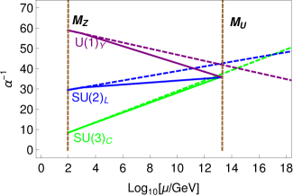
Figure 1: Evolution of the gauge coupling constants of SM gauge symmetry, where dashed lines are contributions from SM particle content and solid lines correspond to RGEs with SM plus $R_{2}$ and $\Sigma$. The vertical dotted lines from left-right are representing symmetry breaking scales $M_{Z}$ as electroweak scale and $M_{U}$ as unification scale.

We skip the discussion RG evolution of gauge coupling constants with two loop effects. While the one-loop RGEs from mass scale $M_{Z}$ to $M_{I}$ and $M_{I}$ to $M_{U}$ are read as follows,

$$\alpha^{-1}_{i}(M_{Z}) =\alpha^{-1}_{i}(M_{I})+\frac{b_{i}}{2\pi}{\large\ln}\left(\frac{M_{I}}{M_{Z}}\right),\,$$

$$\alpha^{-1}_{i}(M_{I}) =\alpha^{-1}_{i}(M_{U})+\frac{b^{\prime}_{i}}{2\pi}{\large\ln}\left(\frac{M_{U}}{M_{I}}\right).$$ (7)

Simplifying RGEs, we obtain the analytic solution for unification mass scale as

$${\large\ln}\left(\frac{M_{U}}{M_{Z}}\right)=\frac{A_{I}D_{W}-B_{I}D_{S}}{B_{U}A_{I}-B_{I}A_{U}},$$ (8)

where, the parameters $D_{S}$ and $D_{W}$ are given by

$$D_{S}=16\pi\left[\alpha_{S}^{-1}(M_{Z})-\frac{3}{8}\alpha^{-1}_{\rm em}(M_{Z})\right]\,,~{}~{}D_{W}=16\pi\left[\sin^{2}\theta_{W}-\frac{3}{8}\right]\alpha^{-1}_{\rm em}(M_{Z}).$$ (9)

While all other parameters are expressed in terms of one-loop beta coefficients as

$$A_{I}=\Bigg{[}\Big{(}8b_{3C}-3b_{2L}-5b_{Y}\Big{)}-\Big{(}8b_{3C}^{{}^{\prime}}-3b_{2L}^{{}^{\prime}}-5b_{Y}^{{}^{\prime}}\Big{)}\Bigg{]},~{}~{}A_{U}=\left(8b_{3C}^{{}^{\prime}}-3b_{2L}^{{}^{\prime}}-5b_{Y}^{{}^{\prime}}\right),$$

$$B_{I}=\left[\left(5b_{2L}-5b_{Y}\right)-\left(5b_{2L}^{{}^{\prime}}-5b_{Y}^{{}^{\prime}}\right)\right],~{}~{}B_{U}=\Big{(}5\,b^{\prime}_{2L}-5\,b^{\prime}_{Y}\Big{)}.$$ (10)

Using the experimental values of $\alpha_{\rm em}$, $\alpha_{\rm S}$, $M_{Z}$ and Weinberg mixing angle Olive et al. (2014); Mou and Zheng (2017), the estimated values of unification mass scale and inverse GUT coupling constant are given by

$$M_{U}=10^{13.27}\,\,\mbox{GeV and}\quad\alpha^{-1}_{U}=36.287.$$ (11)

The evolution of gauge couplings for $SU(3)_{C}$, $SU(2)_{L}$ and $U(1)_{Y}$ gauge groups are displayed in Fig.1. Here, the dashed (solid) lines correspond to SM contribution (SM plus $R_{2}$ and $\Sigma$ contributions). The purple line refers to inverse fine structure constant for $U(1)_{Y}$ group while blue and green lines correspond to $SU(2)_{L}$ and $SU(3)_{C}$ groups respectively. It is evident that the SM predictions with dashed lines demonstrate that there is no such gauge coupling unification. However, with the inclusion of extra particles on top of SM at TeV scale, evolution of gauge couplings begin to deviate from the SM results and provide successful gauge coupling unification of weak, electromagnetic and strong forces.

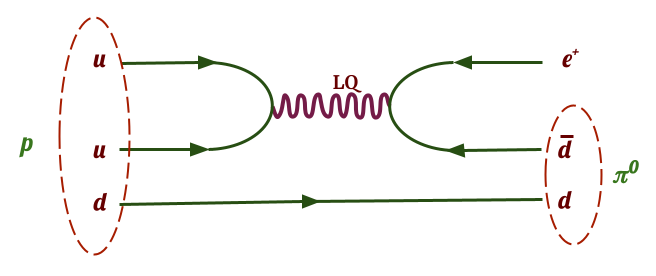
Figure 2: Proton decay mediated by leptoquark gauge bosons contained in adjoint representation of $SO(10)$.

II.1 Prediction of proton lifetime

The interesting feature of grand unified theories is that they can have a robust prediction on proton decay with the presence of exotic interactions mediated by super heavy gauge bosons and scalars. Most commonly discussed gauge boson mediated proton decay arises from the covariant derivative of the fermions in $16_{F}$ with the gauge bosons contained in $45_{V}$ of $SO(10)$, leading to the interaction between quarks and leptons. In our framework, we assume that dominant contributions to proton decay to a neutral pion and a positron comes from the mediation of leptoquark gauge bosons in $45_{V}$. For simplicity, we neglect the contributions form other super heavy particles.

The gauge boson mediated proton life time in the process $p\to e^{+}\pi^{0}$  Babu and Mohapatra (1993); Bertolini et al. (2013); Koleˇsová and Malinský (2014); Parida et al. (2017); Meloni et al. (2019); Ibanez and Munoz (1984); Buras et al. (1978); Bhupal Dev and Mohapatra (2010); Chakrabortty et al. (2019); Babu and Khan (2015) shown in Fig. 2, is given by

$$\tau_{p}={\Gamma}^{-1}\left(p\rightarrow\pi^{0}e^{+}\right) = \frac{64\pi f^{2}_{\pi}}{m_{p}}\left(\frac{M^{4}_{U}}{g^{4}_{U}}\right)\times\frac{1}{|{A_{L}}|^{2}|\overline{\alpha}_{H}|^{2}\left(1+\mathcal{F}+\mathcal{D}\right)^{2}{\mathcal{R}}}.$$ (12)

Here, $g_{U}$ is the GUT scale coupling related with fine structure constant as $\alpha_{U}=g_{U}^{2}/4\pi$ and the predicted unification mass scale $M_{U}$ is the typical mass scale of all the super heavy particles. The other parameters, like $m_{p}$ stands for proton mass, $f_{\pi}$ is the pion decay constant ${\mathcal{R}}$ is the renormalization factor, ${\mathcal{R}}=\left({A_{SL}}^{2}+{A_{SR}}^{2}\right)\left(1+|{V_{ud}}|^{2}\right)^{2}\$ with $V_{ud}$ being the CKM-matrix element. Defining ${A^{2}_{R}}={A^{2}_{L}}\left({A^{2}_{SL}}+{A^{2}_{SR}}\right)$ and $\alpha_{H}=\overline{\alpha}_{H}\left(1+\mathcal{F}+\mathcal{D}\right)$, the proton lifetime is modified as follows

$$\tau_{p\rightarrow\pi^{0}e^{+}} = \frac{4}{\pi}\left(\frac{f^{2}_{\pi}}{m_{p}}\right)\left(\frac{M^{4}_{U}}{\alpha^{2}_{U}}\right)\frac{1}{\alpha^{2}_{H}{A^{2}_{R}}\left(1+|{V_{ud}}|^{2}\right)^{2}}\,.$$ (13)

In the present model, the long distance enhancement factor is $A_{L}\simeq 1.25$ while the short distance renormalization factors are $A_{SL}=2.46$ and $A_{SR}=2.34$. Using $\alpha_{H}=0.012$ GeV³ and the estimated values of $M_{U}$ and $\alpha_{U}$, the proton lifetime is found to be

$$\tau_{p}=4.16925\times 10^{24}~{}{\rm yrs}.$$ (14)

This prediction is well below the current bound set by Super-Kamiokande Abe et al. (2017) ($\tau^{\rm SK}_{p}>1.6\times 10^{34}\,\mbox{yrs}$) and Hyper-Kamiokande Abe et al. (2011); Yokoyama (2017) ($\tau_{p}^{\rm HK2025}>9.0\times 10^{34}\,\mbox{yrs}$). The gravitational corrections arising from higher dimensional operators or GUT threshold effects can enhance the unification mass scale $M_{U}$ and the proton lifetime, consistent with the experimental bounds.

In the next section, we will estimate the one-loop GUT threshold contributions to evolution of gauge coupling constants starting from derived unification mass scale $M_{U}$. As a result, we get a threshold corrected unification mass scale $M^{TH}_{U}$ and also examine whether the corrected proton lifetime is in agreement with the experimental constraints.

III GUT threshold predictions on unification scale and proton decay

The idea of one-loop GUT threshold corrections is to shift the values of SM gauge couplings at $M_{U}$ with the presence of super heavy particles. For illustration, let us consider the minimal $SO(10)$ Higgs representation as $10_{S}\equiv\phi(1,2,1/2)+S_{1}(1,2,-1/2)+S_{2}(3,1,-1/3)+S_{3}(3,1,1/3)$. Since, $\phi$ is utilized at low scale for electroweak symmetry breaking, all other scalars are considered as super heavy scalars and may contribute to the one-loop GUT threshold corrections. The same argument can be applied to other scalars/fermions/gauge bosons contained in different representation of $SO(10)$ presented in the Table. 3.

Table 3: Super heavy scalars, fermions and vector bosons contributing to the GUT threshold corrections.

	$SM$	$G_{321}$
Scalars	$10_{S}$	$S_{1}(\boldsymbol{1},\boldsymbol{2},-1/2)$, $S_{2}(\boldsymbol{3},\boldsymbol{1},-1/3)$, $S_{3}(\overline{\boldsymbol{3}},\boldsymbol{1},1/3)$ ,
	$126_{S}$	$2S_{4}(\boldsymbol{3},\boldsymbol{1},-1/3)$, $S_{5}(\overline{\boldsymbol{3}},\boldsymbol{1},1/3)$, $S_{6}(\boldsymbol{1},\boldsymbol{3},1)$, $S_{7}(\overline{\boldsymbol{6}},\boldsymbol{3},-1/3)$ , $S_{8}(\boldsymbol{1},\boldsymbol{1},0)$
		$S_{9}(\boldsymbol{1},\boldsymbol{1},-1)$, $S_{10}(\boldsymbol{1},\boldsymbol{1},-2)$, $S_{11}(\boldsymbol{3},\boldsymbol{1},2/3)$, $S_{12}(\boldsymbol{3},\boldsymbol{1},-4/3)$, $S_{13}(\boldsymbol{6},\boldsymbol{1},4/3)$
		$S_{14}(\boldsymbol{6},\boldsymbol{1},1/3)$, $S_{15}(\boldsymbol{6},\boldsymbol{1},2/3)$, $S_{16}(\boldsymbol{1},\boldsymbol{2},1/2)$, $S_{17}(\boldsymbol{1},\boldsymbol{2},-1/2)$, $S_{18}(\boldsymbol{3},\boldsymbol{2},1/6)$
		$S_{19}(\overline{\boldsymbol{3}},\boldsymbol{2},-7/6)$, $S_{20}(\overline{\boldsymbol{3}},\boldsymbol{2},-1/6)$, $S_{21}(\boldsymbol{8},\boldsymbol{2},1/2)$, $S_{22}(\boldsymbol{8},\boldsymbol{2},-1/2)$, $S_{23}(\overline{\boldsymbol{3}},\boldsymbol{3},1/3)$
Fermions	${16}_{F}$
	${45}_{F}$	$F_{1}(\boldsymbol{1},\boldsymbol{1},1)$, $2F_{2}(\boldsymbol{1},\boldsymbol{1},0)$, $F_{3}(\boldsymbol{1},\boldsymbol{1},-1)$, $F_{4}(\boldsymbol{3},\boldsymbol{2},1/6)$, $F_{5}(\boldsymbol{3},\boldsymbol{2},-5/6)$
		$F_{6}(\overline{\boldsymbol{3}},\boldsymbol{2},5/6)$, $F_{7}(\overline{\boldsymbol{3}},\boldsymbol{2},-1/6)$, $F_{8}(\boldsymbol{3},\boldsymbol{1},2/3)$, $F_{9}(\overline{\boldsymbol{3}},\boldsymbol{1},-2/3)$, $F_{10}(\boldsymbol{8},\boldsymbol{1},0)$
Vectors	$45_{V}$	$V_{1}(\boldsymbol{1},\boldsymbol{1},1)$, $V_{2}(\boldsymbol{1},\boldsymbol{1},0)$, $V_{3}(\boldsymbol{1},\boldsymbol{1},-1)$, $V_{4}(\boldsymbol{3},\boldsymbol{2},1/6)$, $V_{5}(\boldsymbol{3},\boldsymbol{2},-5/6)$
		$V_{6}(\overline{\boldsymbol{3}},\boldsymbol{2},5/6)$, $V_{7}(\overline{\boldsymbol{3}},\boldsymbol{2},-1/6)$, $V_{8}(\boldsymbol{3},\boldsymbol{1},2/3)$, $V_{9}(\overline{\boldsymbol{3}},\boldsymbol{1},-2/3)$

III.1 Analytic formula for threshold corrections

The matching condition at a given symmetry breaking scale $\mu$, by including one-loop GUT threshold corrections is given by Hall (1981); Parida et al. (2017); Chakrabortty et al. (2019); Babu and Khan (2015); Schwichtenberg (2019)

$$\alpha^{-1}_{D}(\mu)=\alpha^{-1}_{P}(\mu)-\frac{{\lambda_{D}(\mu)}}{12\pi},$$ (15)

where $\alpha_{P}^{-1}(\mu)$ and $\alpha_{D}^{-1}(\mu)$ denote the inverse coupling constant corresponding to the parent and daughter gauge groups. The parent gauge symmetry gets spontaneously broken down to the daughter gauge group at the mass scale $\mu=M_{U}$, where, the parent group is a simple $SO(10)$ and the daughter one is a product of different gauge symmetries i.e, $SU(3)_{C}\times SU(2)_{L}\times U(1)_{Y}$. In the present model, the matching conditions for all the inverse gauge couplings of SM at $M_{U}$ are read as

$$\alpha^{-1}_{i}(M_{U})=\alpha^{-1}_{U}(M_{U})-\frac{{\lambda_{i}(M_{U})}}{12\pi}.$$ (16)

The threshold parameter ${\lambda_{i}}$ is a sum of individual contributions due to the presence of super heavy scalars, fermions and vector bosons (or gauge bosons) with masses $M_{S}$, $M_{F}$ and $M_{V}$ respectively at GUT scale, is given by

$$\lambda_{i}(M_{U})=\lambda^{S}_{i}(M_{U})+\lambda^{F}_{i}(M_{U})+\lambda^{V}_{i}(M_{U}),$$ (17)

where,

$$\lambda^{S}_{i}(M_{U})=\sum_{j}2\,k\mbox{\large Tr}\left[t_{i}^{2}(S_{j})\large{\large\ln}\left(\frac{M_{S_{j}}}{M_{U}}\right)\right],$$

$$\lambda^{F}_{i}(M_{U})=\sum_{j}8\,\kappa\mbox{\large Tr}\left[t^{2}_{i}(F_{j})\large{\large\ln}\left(\frac{M_{F_{j}}}{M_{U}}\right)\right],$$

$$\lambda^{V}_{i}(M_{U})=\mbox{\large Tr}\left[t_{i}^{2}(V_{j})\right]-21\sum_{j}2\,k\mbox{\large Tr}\left[t_{i}^{2}(V_{j})\large{\large\ln}\left(\frac{M_{V_{j}}}{M_{U}}\right)\right].$$ (18)

Here $t_{i}$ represents the generators of the super heavy particles under the $i^{\rm th}$ gauge group. Also the other factors are $k=\frac{1}{2}(1)$ for real (complex) scalars and $\kappa=\frac{1}{2}(1)$ is for Weyl (Dirac) fermions. Now, using the threshold effects in RGEs and after simplifications, one can derive the corrected unification mass scale as follows

$${\large\ln}\left(\frac{M_{U}}{M_{Z}}\right)=\frac{A_{I}{D_{W}}-B_{I}{D_{S}}}{B_{U}A_{I}-B_{I}A_{U}}+\frac{A_{I}{f^{U}_{B}}-B_{I}{f^{U}_{A}}}{B_{U}A_{I}-B_{I}A_{U}}$$

$$\hskip 46.94687pt={\large\ln}\left(\frac{M_{U}}{M_{Z}}\right)_{1-{\rm loop}}+{\Delta}{\large\ln}\left(\frac{M_{U}}{M_{Z}}\right)_{\rm GUT-Th.}.$$ (19)

First term is the contribution from one-loop RGEs while the second term is for threshold corrections. The one-loop threshold corrections are contained in parameters like ${f^{U}_{A}}$ and ${f^{U}_{B}}$ which depend on ${\lambda}$’s as, ${f^{U}_{A}}=\left(8{\lambda^{U}_{3C}}-3{\lambda^{U}_{2L}}-5{\lambda^{U}_{Y}}\right)/6$ and ${f^{U}_{B}}=\left(5{\lambda^{U}_{2L}}-5{\lambda^{U}_{Y}}\right)/6$. This simplifies the corrections as

$${\Delta}{\large\ln}\left(\frac{M_{U}}{M_{Z}}\right) = \frac{1}{700}\bigg{[}15{\lambda^{U}_{Y}}(M_{U})-13{\lambda^{U}_{2L}}(M_{U})-2{\lambda^{U}_{3C}}(M_{U})\bigg{]}.$$ (20)

For degenerate masses for super heavy fields:-  For the estimation of threshold effects arising from super heavy particles, we assume that all the the super heavy gauge bosons have same mass but different from GUT symmetry breaking scale. The same assumption is also applicable to all other super heavy scalars and fermions. The estimated individual threshold corrections are

$${\lambda^{U}_{3C}}(M_{U}) =5-105\eta_{V}+70\eta_{S}+64\eta_{F},$$

$${\lambda^{U}_{2L}}(M_{U}) =6-126\eta_{V}+68\eta_{S}+48\eta_{F},$$

$${\lambda^{U}_{Y}}(M_{U}) =8-168\eta_{V}+\frac{308}{5}\eta_{S}+64\eta_{F}.$$ (21)

Here, $\eta_{S}=\mbox{ln}\frac{M_{S}}{M_{U}}$, $\eta_{F}=\mbox{ln}\frac{M_{F}}{M_{U}}$ and $\eta_{V}=\mbox{ln}\frac{M_{V}}{M_{U}}$. Using these values, the relation for unification mass scale with GUT threshold corrections is modified as,

$${\Delta}{\large\ln}\left(\frac{M_{U}}{M_{Z}}\right)=\frac{1}{175}\bigg{[}8-168\,\eta_{V}-25\,\eta_{S}+52\,\eta_{F}\bigg{]}.$$ (22)

We have presented few benchmark points in Table. 4 for degenerate spectrum of super heavy particles and estimated the unification mass scale and proton lifetime including the threshold effects.

$\boldsymbol{\frac{M_{V}}{M_{U}}}$	$\boldsymbol{\frac{M_{S}}{M_{U}}}$	$\boldsymbol{\frac{M_{F}}{M_{U}}}$	$\boldsymbol{\lambda_{3C}}$	$\boldsymbol{\lambda_{2L}}$	$\boldsymbol{\lambda_{Y}}$	$\boldsymbol{M_{U}^{TH}}$ [GeV]	$\boldsymbol{\tau_{p}}$ [yrs]
$\frac{1}{500}$	$1.5$	$\frac{1}{10}$	$538.531$	$706.062$	$929.631$	$10^{15.5598}$	$6.88124\times 10^{33}$
$\frac{1}{600}$	$2.0$	$\frac{1}{10}$	$577.811$	$748.596$	$977.981$	$10^{15.6179}$	$1.17508\times 10^{34}$
$0.00123$	$2.03634$	$0.10048$	$610.978$	$787.971$	$1029.96$	$10^{15.7429}$	$3.71592\times 10^{34}$
$0.00107$	$1.90066$	$0.10013$	$619.977$	$799.971$	$1047.96$	$10^{15.8025}$	$6.43379\times 10^{34}$
$0.00060$	$1.6374$	$0.0628$	$640.976$	$840.969$	$1106.96$	$10^{15.9948}$	$3.78152\times 10^{35}$
$0.00045$	$16.989$	$0.0784$	$849.969$	$1047.96$	$1314.95$	$10^{16.0017}$	$4.02964\times 10^{35}$

Table 4: Numerically estimated values for $M_{U}$ and ${\tau}_{p}$ by considering one-loop threshold effects.

For non-degenerate masses for super heavy vector bosons:-  Here, we assume all super heavy color triplet and color singlet gauge bosons are non-degenerate but different from GUT symmetry breaking scale, while other super heavy scalars and fermions are degenerate. With new parameters like $\eta_{V_{C}}$ and $\eta_{V_{NC}}$ along with $\eta_{S}$ and $\eta_{F}$, the individual threshold corrections are estimated to

$${\lambda^{U}_{3C}}(M_{U}) =5-21\left(5\eta_{V_{C}}+0\eta_{V_{NC}}\right)+70\eta_{S}+64\eta_{F},$$

$${\lambda^{U}_{2L}}(M_{U}) =6-21\left(6\eta_{V_{C}}+0\eta_{V_{NC}}\right)+68\eta_{S}+48\eta_{F},$$

$${\lambda^{U}_{Y}}(M_{U}) =8-21\left(\frac{34}{5}\eta_{V_{C}}+\frac{6}{5}\eta_{V_{NC}}\right)+\frac{308}{5}\eta_{S}+64\eta_{F}.$$ (23)

where,

$$\eta_{S}=\mbox{ln}\frac{M_{S}}{M_{U}},\eta_{F}=\mbox{ln}\frac{M_{F}}{M_{U}},\eta_{V_{C}}=\mbox{ln}\frac{M_{V_{C}}}{M_{U}},\eta_{V_{NC}}=\mbox{ln}\frac{M_{V_{NC}}}{M_{U}}.$$

The notation $M_{VC}$ and $M_{V_{NC}}$ are the degenerate masses of the vector gauge bosons $V_{4}$ to $V_{9}$ and $V_{1}$ to $V_{3}$ respectively (shown in Table. 3). Using these input values, GUT threshold corrected unification mass scale is given by

$${\Delta}{\large\ln}\left(\frac{M_{U}}{M_{Z}}\right)=\frac{1}{350}\bigg{[}16-147\,\eta_{V_{C}}-189\,\eta_{V_{NC}}-50\,\eta_{S}+104\,\eta_{F}\bigg{]}.$$ (24)

$\boldsymbol{\frac{M_{V_{C}}}{M_{U}}}$	$\boldsymbol{\frac{M_{V_{NC}}}{M_{U}}}$	$\boldsymbol{\frac{M_{S}}{M_{U}}}$	$\boldsymbol{\frac{M_{F}}{M_{U}}}$	$\boldsymbol{\lambda_{3C}}$	$\boldsymbol{\lambda_{2L}}$	$\boldsymbol{\lambda_{Y}}$	$\boldsymbol{M_{U}^{TH}}$ [GeV]	$\boldsymbol{\tau_{p}}$ [yrs]
$\frac{1}{400}$	$\frac{1}{100}$	$2.0$	$0.3$	$617.914$	$765.08$	$962.059$	$10^{15.287}$	$5.57785\times 10^{32}$
$\frac{1}{2500}$	$\frac{1}{100}$	$2.5$	$0.5$	$846.273$	$1020.83$	$1253.36$	$10^{15.6519}$	$1.60719\times 10^{34}$
$\frac{1}{3000}$	$\frac{1}{300}$	$1.5$	$0.25$	$785.299$	$975.796$	$1231.25$	$10^{15.885}$	$1.37552\times 10^{35}$
$\frac{1}{4000}$	$\frac{1}{400}$	$0.5$	$0.2$	$724.324$	$926.629$	$1197.63$	$10^{16.044}$	$5.94931\times 10^{35}$
$\frac{1}{5000}$	$\frac{1}{400}$	$0.15$	$0.2$	$663.479$	$872.877$	$1155.33$	$10^{16.16}$	$1.73168\times 10^{36}$
$\frac{1}{2000}$	$\frac{1}{500}$	$\frac{1}{2500}$	$0.1$	$108.042$	$321.143$	$620.668$	$10^{16.323}$	$7.77082\times 10^{36}$

Table 5: Numerically estimated values of $M_{U}$ and ${\tau}_{p}$ by including one-loop threshold effects by considering non-degenerate masses for super heavy vector bosons.

In Table 5, we have presented various mass values for gauge bosons, scalars and fermions and estimated the threshold corrected unification mass scale and the corresponding proton lifetime. The evolution of gauge coupling constants including one-loop threshold corrections is shown in Fig. 3 by considering the benchmark given the last row of Table. 5. The corresponding corrected unification mass scale and proton lifetime consistent with Super-Kamiokande Abe et al. (2017)and Hyper-Kamiokande Abe et al. (2011); Yokoyama (2017), are

$$M_{U}^{TH}=10^{16.323}\,\mbox{GeV},\quad\tau_{p}=7.77082\times 10^{36}\mbox{yrs}.$$ (25)

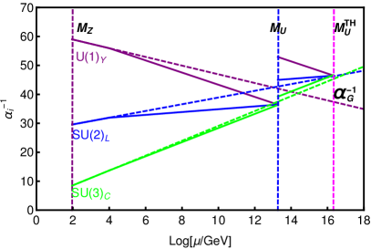
Figure 3: Unification plot for all three gauge couplings, where the one-loop effects are displayed upto the mass scale $M_{U}$ while the threshold effects are shown in the mass range $M_{U}-M_{U}^{TH}$.

IV Discussion on fermion masses and mixing

It has been pointed in Witten’s work Witten (1980) that the minimal non-supersymmetric $SO(10)$ model with only $10_{H}$ (containing SM Higgs) and $16_{F}$ (accommodating SM fermions plus right-handed neutrinos) predicts $m_{d}\simeq m_{e}$, $m_{s}\simeq m_{\mu}$, which are ruled out from experiments. In this scenario, the neutrinos have only Dirac masses proportional to up-type quark masses which disagree with the current neutrino oscillation data. Moreover, there is a possibility to have small Majorana masses for right-handed neutrinos via two-loop effects using $16_{H}$ on top of $10_{H}$. Thus, the failure of $SO(10)$ model to account correct fermion masses and mixing motivates us to explore all possible non-minimal scenarios.

The correct fermion masses and mixing can be addressed in non-supersymmetric $SO(10)$ theory with the inclusion of extra $10_{H}$ Bajc et al. (2006) while $126_{H}$ was introduced for breaking of Pati-Salam symmetry or left-right symmetry as an intermediate symmetry between $SO(10)$ theory and SM Babu and Ma (1985); Anastaze et al. (1983); Yasue (1981a, b); Bertolini et al. (2009b); Bertolini et al. (2010); Bajc et al. (2006); Altarelli and Meloni (2013b); Dueck and Rodejohann (2013b); Joshipura and Patel (2011); Babu et al. (2017); Ohlsson and Pernow (2018). In our present work, we adopt two $10_{H}$ and one $126_{H}$ representation along with $16_{F}$ and $45_{F}$ in the fermion sector in order to explain fermion masses and mixing, dark matter and flavor physics anomalies. The SM Higgs can be admixture of two Higgs doublets contained in two $10_{H}$’s and also from $126_{H}$. We assume that Pati-Salam symmetry of left-right symmetry is broken at GUT breaking scale and that is the reason why we are expecting the right-handed neutrinos as well as scalar triplets can have their masses around $10^{13}$ GeV close to $M_{U}$. With this, we have not considered its effects while numerically examining the renormalization evolution equation for gauge couplings.

The $SO(10)$ invariant Yukawa interactions are

$$\mathcal{L}_{Y}=16^{i}_{F}\left(Y^{ij}_{10}\,10_{H}+Y^{ij}_{126}\overline{126_{H}}\right)16^{j}_{F}+M_{45}45_{F}45_{F}+{\rm h.c}.,$$ (26)

where $Y_{10}$ and $Y_{126}$ are complex symmetric matrices. Here, $SO(10)$ or equivalent Pati-Salam symmetry ($SU(4)_{C}\times SU(2)_{L}\times SU(2)_{R}$) is broken down at the predicted unification mass scale $10^{13.27}$ GeV. As a result, since the right-handed symmetry breaking scale is close to $M_{U}$, the right-handed neutrinos as well scalar triplets have their masses around that scale, which can generate neutrino masses and mixing via type-I and type-II seesaw mechanisms respectively.

Using two real representations $10_{H_{1}}$ and $10_{H_{2}}$, an equivalent complex $10_{H}$ can be constructed as $10_{H}=10_{H_{1}}+i\,10_{H_{2}}$, without effecting the evolution of gauge couplings. Additionally, we introduce a global Pecci-Quinn symmetry forbidding the Yukawa couplings involving $10^{*}_{H}$ Peccei and Quinn (1977a, b). The $U(1)_{PQ}$ transformation of the relevant $SO(10)$ representations are as follows,

$$16_{F}\to e^{i\,\alpha}16_{F},\quad 45_{F}\to 45_{F},\,$$

$$10_{H}\to e^{-2i\,\alpha}10_{H},\quad\overline{126_{H}}\to e^{-2i\,\alpha}\overline{126_{H}}\,.$$ (27)

As a result of this Pecci-Quinn symmetry, we have two separate vevs (vacuum expectation values) $v_{u,d}^{10}\subset 10_{H}$ and one Yukawa coupling $Y_{10}$. The other advantage of Pecci-Quinn symmetryBoucenna et al. (2019) is to solve strong CP problem and provide axion dark matter Mohapatra and Senjanovic (1983); Marsh (2016); Shafi and Stecker (1984); Jeong et al. (2022); Weinberg (1978); Wilczek (1978); Ringwald (2012); Graham et al. (2015); Arias et al. (2012); Langacker et al. (1986).

The Yukawa terms for fermion masses and mixing, relevant at the PS symmetry breaking scale are given by

$$\mathcal{L}^{\rm PS}_{\rm Yuk}=Y^{ij}_{10_{F}}F^{i^{T}}_{L}\Phi F^{j}_{R}+\widetilde{Y}^{ij}_{10_{F}}F^{i^{T}}_{L}\widetilde{\Phi}F^{j}_{R}+Y^{ij}_{126_{F}}F^{i^{T}}_{L}\overline{\xi}F^{j}_{R}+Y^{ij}_{126_{R}}F^{i^{T}}_{R}\overline{\Delta}_{R}F^{j}_{R}+M_{\Sigma}\Sigma_{F}\Sigma_{F}+{\rm h.c}.$$

The details of mapping of Yukawa couplings at $SO(10)$ and Pati-Salam symmetry can be understood by solving RGEs and interested reader may refer to  Ohlsson and Pernow (2021). Here we consider the vevs $v_{1}$ and $v_{2}$ from the PS multiplet $(1,2,2)$ of $10_{H}$. The primary role of these vevs (of the order of EW scale) is to generate fermion masses and help in breaking of $SU(3)_{C}\times\,\text{SU}(2)_{L}\times U(1)_{Y}$ down to $SU(3)_{C}\times U(1)_{\rm em}$. The other vevs are relevant for correcting bad mass relations in fermion masses are $\langle\xi\rangle\approx v_{\xi_{1}},v_{\xi_{2}}\subset 126_{H}$ in the MeV scale. As pointed out in ref Babu and Mohapatra (1993), these small induced vevs of Pati-Salam multiplet $(15_{4C},2_{2L},2_{2R})$ are coming from the important scalar interaction term,

$$V=\lambda_{\xi}\,M^{\prime}\,{210}_{H}\,{126}_{H}^{\dagger}\,{10}_{H}\supset\lambda_{\xi}\,M^{\prime}\,{(15,2,2)}_{126}\,{(15,1,1)}_{210}\,{(1,2,2)}_{10}\,,$$

This provides the induced vev $v_{\xi}$ of the neutral component of $\xi(15,2,2)$ as,

$$v_{\xi}=\lambda_{\xi}\,M^{\prime}\,M_{C}\,v_{ew}/M_{\xi}^{2}\,,$$

where, $v_{ew}=\sqrt{v_{1}^{2}+v_{2}^{2}}$. Using these vevs and Yukawa couplings, the fermion masses at electroweak scale can be expressed in terms of Yukawa couplings defined at Pati-Salam scale and various vevs arising from $10_{H}$ and $126_{H}$ are given by

$$M_{u}\equiv v_{u}Y_{u}=v_{1}Y_{10_{F}}^{u}+v_{\xi_{1}}Y_{126_{F}}^{u}\,,\quad M_{d}\equiv v_{d}Y_{d}=v_{2}Y_{10_{F}}^{d}+v_{\xi_{2}}Y_{126_{F}}^{d}\,,$$

$$M_{e}\equiv v^{10}_{d}Y_{e}=v_{2}Y_{10_{F}}^{e}+v_{\xi_{2}}Y_{126_{F}}^{e}\,,\quad M^{D}_{\nu}\equiv v_{u}Y_{\nu}=v_{1}Y_{10_{F}}^{\nu}+v_{\xi_{1}}Y_{126_{F}}^{\nu}\,,$$

$$M_{R}=v_{R}Y^{\nu}_{126_{R}}\,,\quad\big{[}M_{L}=v_{L}Y^{\nu}_{126_{L}}\,\mbox{for $G_{224D}$}\big{]}.$$ (29)

Here, $M_{u}$ ($M_{d}$) denotes the mass matrix for up (down)-type quarks whereas $M_{e}$ represents the mass matrix of the charged leptons. Also $M^{D}_{\nu}$ is Dirac neutrino mass matrix, while $M_{L}$ and $M_{R}$ stand for Majorana mass matrix for light left-handed and heavy right-handed neutrinos respectively. Applying appropriate boundary condition at Pati-Salam symmetry breaking scale, the simplified fermion mass matrices become Babu and Mohapatra (1993),

$$M_{u}=Hv_{1}+Fv_{\xi_{1}}\,,\quad M_{d}=Hv_{2}+Fv_{\xi_{2}}$$

$$M^{D}_{\nu}=Hv_{1}-3Fv_{\xi_{1}}\,,\quad M_{e}=Hv_{2}-3Fv_{\xi_{2}}$$

$$M_{R}=Fv_{R}$$ (30)

Here, $H$ and $F$ are Yukawa coupling matrices derived in terms Yukawa coupling matrices defined at Pati-Salam symmetry. Let us consider a basis where $H$ is real and diagonal. Also define two more parameters; ratio between two Higgs doublet VEVs of $10_{H}$ i.e, $r_{1}=v_{2}/v_{1}$ and ratio between two Higgs doublet VEVs of $126_{H}$ i.e, $r_{2}=v_{\xi_{2}}/v_{\xi_{1}}$. As a result, there are total 13 parameters excluding the VEVs $v_{R}$ (or $v_{L}$) present in the fermion mass fitting: 3 diagonal elements of matrix $H$, 6 elements of symmetric matrix F, 2 ratios of VEVs $r_{1},r_{2}$ and two physical phases $\alpha$ and $\beta$ used in the VEVs. These 13 parameters have been utilised to explain the 13 observables in the charged fermion masses: 9 fermion masses, 3 quark mixing angles and one CP-phase. Also, the resulting Dirac neutrino mass matrix can be expressed in terms of $v_{R}$ and other input model parameters. So, one can rewrite the simplified fermion mass relations in terms of these ratios of different VEVs as follows Babu and Mohapatra (1993),

$$M_{e}=\frac{4r_{1}r_{2}}{r_{2}-r_{1}}M_{u}-\frac{r_{1}+3r_{2}}{r_{2}-r_{1}}M_{d}\,,$$

$$M^{D}_{\nu}=\frac{3r_{1}+r_{2}}{r_{2}-r_{1}}M_{u}-\frac{4}{r_{2}-r_{1}}M_{d}\,$$

$$M_{R}=\frac{1}{R}\frac{r_{1}}{r_{1}-r_{2}}M_{u}-\frac{1}{R}\frac{1}{r_{1}-r_{2}}M_{d}\,,$$ (31)

where $R=v_{1}/v_{R}$. We can consider a basis where $M_{u}$ is already diagonal with masses as $M_{u}=\mbox{Diag}\big{(}m_{u},m_{c},m_{t}\big{)}$. In this choice of basis, the down-type quark mass matrix can be diagonalised by $\hat{M}_{d}\simeq V^{\dagger}_{\rm CKM}M_{d}V_{\rm CKM}=\mbox{Diag}\big{(}m_{d},m_{s},m_{b}\big{)}$ where $V_{\rm CKM}$ is the usual CKM mixing matrix. It is to be noted that the charged lepton mass matrix can now be fully determined in terms of physical observables of quark sector and two parameters related to ratios of various VEVs i.e, $r_{1}$ and $r_{2}$.

Let us consider that the Dirac neutrino mass matrix is approximated to be up-quark mass matrix in the present scenario with the high scale intermediate symmetry as Pati-Salam. Using the seesaw approximation with the mass hierarchy $M_{R}\gg M_{\nu}^{D}\gg M_{L}$, the resulting light neutrino mass formula via type-I seesaw with the PS symmetry without D-parity as the only intermediate symmetry or type-I+II within D-parity conserving PS symmetry, seesaw contributions are as follows

$$M_{\nu}=-M^{D}_{\nu}M^{-1}_{R}M^{D}_{\nu}\,\big{(}+M_{L}\quad\mbox{for}\,G_{422D}\big{)}\,.$$ (32)

For typical value of $M_{R}\sim 10^{13.27}$ GeV, $M^{D}_{\nu}\sim 100$ GeV, we obtain sub-eV mass for light neutrinos. The out-of-equilibrium decays of right-handed neutrinos can provide the observed baryon asymmetry of the Universe via type-I leptogenesis. We skip the details of fermion mass fitting and its implications to matter-antimatter asymmetry of the universe which can be looked up in recent works Babu and Mohapatra (1993); Mummidi and Patel (2021).

V Addressing flavor anomalies with scalar leptoquark $R_{2}$

It has been already examined that inclusion of TeV scale SLQ and a fermion triplet DM candidate leads to successful unification of the gauge coupling, when embedded in a non-supersymmetric $SO(10)$ GUT. The presence of TeV scale SLQ arising from GUT framework has interesting low-energy phenomenology like explaining flavor anomalies, muon $g-2$, collider studies etc Babu et al. (2021). However, in the present work, we stick with discussions of phenomenological implications of SLQ to recent flavor anomalies in semileptonic $B$ decays. In recent times, several intriguing deviations at $(2-4)\sigma$ significance level, have been realized by the three pioneering experiments: Babar Lees et al. (2012a, 2013), Belle Huschle et al. (2015); Hirose et al. (2017); Abdesselam et al. (2019a); Abdesselam et al. (2019b, 2021) and LHCb Aaij et al. (2013b, a, 2014b, 2014a, 2015a, 2015b, 2017, 2018b, 2018a, 2019a), in the form of lepton flavour universality (LFU) violation associated with the charged-current (CC) and neutral-current (NC) transitions in semileptonic $B$ decays. These discrepancies can’t be accommodated in the SM and are generally interpreted as smoking-gun signals of NP contributions. The discrepancies in the CC sector are usually attributed to the presence of new physics in $b\to c\tau\bar{\nu}_{\tau}$ transition, whereas in the NC sector to $b\to s\mu\mu$ process. It has been shown in the literature that various leptoquark scenarios can successfully address these anomalies. Here, we will show that $R_{2}(3,2,7/6)$ leptoquark present in our model can successfully explain these discrepancies.

The generalized effective Hamiltonian accountable for the charged-current $b\to c\tau\bar{\nu}_{\ell}$ transitions is given as Tanaka and Watanabe (2013)

$$\mathcal{H}_{\rm eff}^{\rm CC}\ =\ \frac{4G_{F}}{\sqrt{2}}V_{cb}\Big{[}\left(\delta_{\ell\tau}+C_{V_{1}}^{\ell}\right)\mathcal{O}_{V_{1}}^{\ell}+C_{V_{2}}^{\ell}\mathcal{O}_{V_{2}}^{\ell}+C_{S_{1}}^{\ell}\mathcal{O}_{S_{1}}^{\ell}+C_{S_{2}}^{\ell}\mathcal{O}_{S_{2}}^{\ell}+C_{T}^{\ell}\mathcal{O}_{T}^{\ell}\Big{]},$$ (33)

where $G_{F}$ and $V_{cb}$ represent the Fermi constant and the Cabibbo-Kobayashi-Maskawa (CKM) matrix element respectively. $C_{X}^{\ell}$ are the new Wilson coefficients, with $X=V_{1,2},S_{1,2},T$, which can arise only when NP prevails. The corresponding four-fermion operators ${\cal O}_{X}^{\ell}$ can be expressed as

$$\mathcal{O}_{V_{1}}^{\ell}\ =\ \left(\bar{c}_{L}\gamma^{\mu}b_{L}\right)\left(\bar{\tau}_{L}\gamma_{\mu}\nu_{\ell L}\right),\qquad\mathcal{O}_{V_{2}}^{\ell}\ =\ \left(\bar{c}_{R}\gamma^{\mu}b_{R}\right)\left(\bar{\tau}_{L}\gamma_{\mu}\nu_{\ell L}\right),$$

$$\mathcal{O}_{S_{1}}^{\ell}\ =\ \left(\bar{c}_{L}b_{R}\right)\left(\bar{\tau}_{R}\nu_{\ell L}\right),\qquad\qquad\mathcal{O}_{S_{2}}^{\ell}\ =\ \left(\bar{c}_{R}b_{L}\right)\left(\bar{\tau}_{R}\nu_{\ell L}\right),$$

$$\mathcal{O}_{T}^{\ell}\ =\ \left(\bar{c}_{R}\sigma^{\mu\nu}b_{L}\right)\left(\bar{\tau}_{R}\sigma_{\mu\nu}\nu_{\ell L}\right)\,,$$ (34)

where $f_{L(R)}=P_{L(R)}f$ with $P_{L(R)}=(1\mp\gamma_{5})/2$, represent the chiral fermion fields $f$.

The effective Hamiltonian delineating the NC transitions $b\to s\ell^{+}\ell^{-}$ is given as Misiak (1993); Buras and Munz (1995)

$${\cal H}_{\rm eff}^{\rm NC}\ =\ -\frac{4G_{F}}{\sqrt{2}}V_{tb}V_{ts}^{*}\Bigg{[}\sum_{i=1}^{6}C_{i}(\mu)\mathcal{O}_{i}+\sum_{i=7,9,10,S,P}\Big{(}C_{i}(\mu)\mathcal{O}_{i}+C_{i}^{\prime}(\mu)\mathcal{O}_{i}^{\prime}\Big{)}\Bigg{]}\;,$$ (35)

where $V_{tb}V_{ts}^{*}$ represents the product of CKM matrix elements, $C_{i}$’s denote the Wilson coefficients and $\mathcal{O}_{i}$’s are the four-fermion operators expressed as:

$$\mathcal{O}_{7}^{(\prime)} \ =\ \frac{\alpha_{\rm em}}{4\pi}\bigg{[}\bar{s}\sigma_{\mu\nu}\big{\{}m_{s}P_{L(R)}+m_{b}P_{R(L)}\big{\}}b\bigg{]}F^{\mu\nu},$$

$$\mathcal{O}_{9}^{(\prime)} \ =\ \frac{\alpha_{\rm em}}{4\pi}\big{(}\bar{s}\gamma^{\mu}P_{L(R)}b\big{)}(\bar{\ell}\gamma_{\mu}\ell)\;,\qquad\mathcal{O}_{10}^{(\prime)}\ =\ \frac{\alpha_{\rm em}}{4\pi}\big{(}\bar{s}\gamma^{\mu}P_{L(R)}b\big{)}(\bar{\ell}\gamma_{\mu}\gamma_{5}\ell)\;,$$

$$\mathcal{O}_{S}^{(\prime)} \ =\ \frac{\alpha_{\rm em}}{4\pi}\big{(}\bar{s}P_{L(R)}b\big{)}(\bar{\ell}\ell)\;,\qquad\qquad\mathcal{O}_{P}^{(\prime)}\ =\ \frac{\alpha_{\rm em}}{4\pi}\big{(}\bar{s}P_{L(R)}b\big{)}(\bar{\ell}\gamma_{5}\ell)\,.$$ (36)

The primed as well as scalar/pseudoscalar operators are absent in the SM and can be generated only in beyond the SM scenarios.

V.1 New contributions with scalar leptoquark

In the context of the present model, the flavour sector will be sensitive to the presence of the SLQ $R_{2}(3,2,7/6)$, which can provide additional contributions to the CC mediated $b\to c\ell\bar{\nu}$ as well as NC $b\to s\ell^{-}\ell^{+}$ processes and can elucidate the observed data reasonably well. The SLQ couples simultaneously to quark and lepton fields through flavor dependent Yukawa couplings and the corresponding interaction Lagrangian can be written as Iguro et al. (2019); Sakaki et al. (2013),

$${\cal L}_{\rm int}=\lambda_{R}^{ij}\overline{Q}_{Li}\ell_{Rj}R_{2}-\lambda_{L}^{ij}\overline{u}_{Ri}R_{2}i\tau_{2}L_{Lj}+{\rm h.c.},$$ (37)

where the couplings $\lambda_{L,R}$ are in general $3\times 3$ complex matrices, $R_{2}=\left(R^{(5/3)}_{2}~{}R^{(2/3)}_{2}\right)^{T}$, $Q_{L}(L_{L})$ represents the left-handed quark (lepton) doublet, $u_{R}(\ell_{R})$ is the right-handed singlet up-type quark (charged lepton) and the generation indices are characterized by $i,j$. The interaction Lagrangian (37) in the mass basis can be obtained after the expanding the $SU(2)$ indices as Iguro et al. (2019)

$${\cal L}_{\rm int} = (V_{\rm CKM}\lambda_{R})^{ij}\overline{u}_{Li}\ell_{Rj}R_{2}^{(5/3)}+\lambda_{R}^{ij}\overline{d}_{Li}\ell_{Rj}R_{2}^{(2/3)}$$ (38)

$$+ \lambda_{L}^{ij}\overline{u}_{Ri}\nu_{Lj}R_{2}^{(2/3)}-\lambda_{L}^{ij}\overline{u}_{Ri}\ell_{Lj}R_{2}^{(5/3)}+{\rm h.c.}.$$

Here the superscripts on $R_{2}$ specify its electric charge and the mass bases for quark doublets are considered as $((V_{\rm CKM}^{\dagger}u_{L})^{i},d_{L}^{i})^{T}$ while for lepton doublets as $(\nu_{L}^{i},\ell_{L}^{i})^{T}$, neglecting the mixing in the lepton sector. Thus, from eqn. (38), one can notice that the exchange of $R_{2}^{(2/3)}$ can induce new contribution to both $b\to c\tau\bar{\nu}_{\tau}$ as well as $b\to s\mu^{-}\mu^{+}$ transitions at tree-level as shown in Fig. 4.

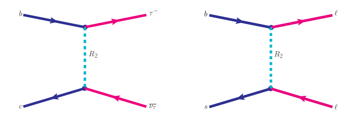
Figure 4: Feynman diagram for the CC transition $b\to c\tau^{-}\bar{\nu}_{\tau}$ (left panel) and NC process $b\to s\ell^{+}\ell^{-}$ (right panel) induced by the scalar leptoquark $R_{2}^{(2/3)}$.

For $b\to c\tau\bar{\nu}_{\tau}$ it generates additional scalar as well as tensor interactions at the LQ mass scale $(\mu=m_{\rm LQ})$ as:

$$C_{S_{2}}^{\rm NP}(m_{\rm LQ})=4C_{T}^{\rm NP}(m_{\rm LQ})=\frac{1}{4\sqrt{2}G_{F}V_{cb}}\frac{\lambda_{L}^{23}(\lambda_{R}^{33})^{*}}{m_{\rm LQ}^{2}}\;,$$ (39)

where $m_{\rm LQ}$ represents the leptoquark mass, and we consider a typical TeV scale SLQ in our analysis. It should be noted that the new Wilson coefficients as shown in eqn. (39) rely on the LQ mass scale $\mu(m_{\rm LQ})$, and hence, it is essential to evolve their values from the $m_{\rm LQ}$ scale to the $b$-quark mass scale $\mu=m_{b}$ through the renormalization-group equation (RGE), which are expressed as Blanke et al. (2019); González-Alonso et al. (2017)

$$\begin{pmatrix}{C_{S_{2}}^{\rm NP}}(m_{b})\\ {C_{T}^{\rm NP}}(m_{b})\end{pmatrix}=\begin{pmatrix}1.752&-0.287\\ -0.004&0.842\end{pmatrix}\begin{pmatrix}{C_{S_{2}}^{\rm NP}}(m_{\rm LQ})\\ {C_{T}^{\rm NP}}(m_{\rm LQ})\end{pmatrix}.$$ (40)

Similarly, after performing the Fierz transformation, the new contribution to the $b\to s\mu^{+}\mu^{-}$ process can be obtained from Eq. (38) as,

$${\cal H}_{\rm LQ} = \frac{\lambda_{R}^{32}{(\lambda_{R}^{22})}^{*}}{8m_{\rm LQ}^{2}}\left(\bar{s}\gamma^{\mu}(1-\gamma_{5})b\right)\left(\bar{\mu}\gamma_{\mu}(1+\gamma_{5})\mu\right)\equiv\frac{\lambda_{R}^{32}{(\lambda_{R}^{22})}^{*}}{4m_{\rm LQ}^{2}}\Big{(}O_{9}+O_{10}\Big{)}.$$ (41)

Thus, comparing (41) with (35), one can obtain the new Wilson coefficients as

$$C_{9}^{\rm NP}=C_{10}^{\rm NP}=-\frac{\pi}{2\sqrt{2}G_{F}\alpha_{\rm em}V_{tb}V_{ts}^{*}}\frac{\lambda_{R}^{32}{(\lambda_{R}^{22})}^{*}}{m_{\rm LQ}^{2}}\;.$$ (42)

After delineating the additional contributions to the Wilson coefficients for the $b\to c\tau\bar{\nu}$ and $b\to s\mu^{+}\mu^{-}$ transitions, we now proceed to constrain the new parameters. We perform a global-fit using all the relevant experimental observables to constrain these new couplings. The list of the observables are provided in the following subsection.

V.2 List of observables used in global-fit

In this analysis, we incorporate the following observables for constraining the new couplings.

1. Observables associated with $\boldsymbol{b\to s\mu^{+}\mu^{-}}$ transitions:

   • $\boldsymbol{R_{K}}$ and $\boldsymbol{R_{K^{*}}}$ : The LFU violating observables $R_{K}$ and $R_{K^{*}}$, expressed as

     $$R_{K}\ =\ \frac{{\rm BR}(B^{+}\to K^{+}\mu^{+}\mu^{-})}{{\rm BR}(B^{+}\to K^{+}e^{+}e^{-})}\,,\qquad R_{K^{*}}\ =\ \frac{{\rm BR}(B^{0}\to K^{*0}\mu^{+}\mu^{-})}{{\rm BR}(B^{0}\to K^{*0}e^{+}e^{-})}\,.$$ (43)

     The recently updated values of $R_{K}$ Aaij et al. (2021) and $R_{K^{*}}$ Aaij et al. (2017), by LHCb experiment in the low $q^{2}$ bins are given as:

     $$R_{K}^{\rm LHCb}=0.846^{+0.044}_{-0.041}\,,\qquad q^{2}\in[1.1,6]~{}{\rm GeV}^{2}\,,$$ (44)

     $$R_{K^{*}}^{\rm LHCb} = \begin{cases}0.660^{+0.110}_{-0.070}\pm 0.024\qquad q^{2}\in[0.045,1.1]~{}{\rm GeV}^{2}\,,\\ 0.685^{+0.113}_{-0.069}\pm 0.047\qquad q^{2}\in[1.1,6.0]~{}{\rm GeV}^{2}\,.\end{cases}$$ (45)

     In addition to the LHCb results, the Belle experiment also has recently reported new measurements on $R_{K}$ Abdesselam et al. (2021) and $R_{K^{*}}$ Abdesselam et al. (2019a) in several other bins. However, as the Belle results have comparatively larger uncertainties, we do not consider them in our fit for constraining the new parameters.

   • $\boldsymbol{B_{s}\to\mu^{+}\mu^{-}}$ :

     The current average value on the branching franction of $B_{s}\to\mu^{+}\mu^{-}$ process from the combined results of ATLAS, CMS and LHCb is  ATL (2020):

     $${\rm BR}(B_{s}^{0}\to\mu^{+}\mu^{-})\ =\ \left(2.69^{+0.37}_{-0.35}\right)\times 10^{-9}\,,$$ (46)

     which has $2.4\sigma$ deviation from its SM prediction Bobeth et al. (2014)

     $${\rm BR}(B_{s}^{0}\to\mu^{+}\mu^{-})^{\rm SM}\ =\ \left(3.65\pm 0.23\right)\times 10^{-9}\,.$$ (47)

   • $\boldsymbol{B\to K^{*}\mu\mu}$ and $\boldsymbol{B_{s}\to\phi\mu\mu}$ processes:

     $\bullet$ We consider the following set of angular observables from $B^{0}\to K^{*0}\mu^{+}\mu^{-}$ process: the form factor independent optimized observables $P_{1,2,3},P_{4,5,6,8}^{\prime}$, the longitudinal polarization fraction $(F_{L})$ and the forward-backward asymmetry $(A_{FB})$ in the following $q^{2}$ bins (in ${\rm GeV}^{2}$): $[0.1,0.98],~{}[1.1,2],~{}[2,3],~{}[3,4],~{}[4,5],~{}[5,6]$ and $[1,6]$ Aaij et al. (2016).
     

     $\bullet$ For $B_{s}\to\phi\mu^{+}\mu^{-}$ mode, we take into account the longitudinal polarization asymmetry $(F_{L})$ and CP averaged observables ($S_{3,4,7},A_{5,6,8,9}$) in the following three $q^{2}$ bins (in ${\rm GeV}^{2}$): $[0.1,2],~{}[2,5]$, and $[1,6]$ Aaij et al. (2015b).

2. $\boldsymbol{b\to c\tau\bar{\nu}_{\tau}}$: For the CC transitions $b\to c\tau\nu$, we incorporate the following observables.

   • $\boldsymbol{R_{D}}$ and $\boldsymbol{R_{D^{*}}}$ : The lepton non-universality observables $R_{D}$ and $R_{D^{*}}$, defined as

     $$R_{D^{(*)}}\ =\ \frac{{\rm BR}(B\to D^{(*)}\tau\bar{\nu}_{\tau})}{{\rm BR}(B\to D^{(*)}\ell\bar{\nu}_{\ell})}\,,$$ (48)

     with $\ell=e,\mu$. These observables are measured by BaBar Lees et al. (2012a, 2013) and Belle Huschle et al. (2015); Hirose et al. (2017); Abdesselam et al. (2016b) whereas only $R_{D^{*}}$ has been measured by LHCb Aaij et al. (2015a, 2018b). The present world-average values of these ratios obtained by incorporating the data from all these measurements are Amhis et al. (2021):

     $$R_{D}^{\rm exp}=0.34\pm 0.027\pm 0.013\,,~{}~{}~{}~{}~{}R_{D^{*}}^{\rm exp}=0.295\pm 0.011\pm 0.008\,,$$ (49)

     exhibit $3.08\sigma$ discrepancy with the corresponding SM results Fajfer et al. (2012a, b)

     $$R_{D}^{\rm SM}\ =\ 0.299\pm 0.003\,,~{}~{}~{}~{}~{}~{}R_{D^{*}}^{\rm SM}\ =\ 0.258\pm 0.005\,.$$ (50)

   • $\boldsymbol{R_{J/\psi}}$ : Analogously, in the measurement of $R_{J/\psi}$ Aaij et al. (2018a)

     $$R_{J/\psi}^{\rm exp}\ =\ \frac{{\rm BR}(B\to J/\psi\tau\bar{\nu}_{\tau})}{{\rm BR}(B\to J/\psi\ell\bar{\nu}_{\ell})}\ =\ 0.71\pm 0.17\pm 0.184\,,$$ (51)

     a discrepancy of about $1.7\sigma$ has been observed with the corresponding SM prediction Ivanov et al. (2005); Wang et al. (2013); Watanabe (2018)

     $$R_{J/\psi}^{\rm SM}\ =\ 0.289\pm 0.01\,.$$ (52)

   • $\boldsymbol{B_{c}^{+}\to\tau^{+}\nu_{\tau}}$ : This leptonic decay process has not been observed so far, however, indirect constraints on ${\rm BR}(B_{c}^{+}\to\tau^{+}\nu_{\tau})\lesssim 30\%$ has been enforced using the lifetime of $B_{c}$ Alonso et al. (2017); Li et al. (2016); Celis et al. (2017).

For the numerical estimation of the SM results of the above-mentioned observables, we use the masses of various particles and the lifetime of $B_{q}$ mesons from PDG Zyla et al. (2020). The SM result for ${\rm BR}(B_{s}\to\mu^{+}\mu^{-})$ is taken from Ref. Bobeth et al. (2014). For evaluating the $B\to K$ transition form factors we use the light cone sum rule (LCSR) approach Ball and Zwicky (2005a) and for $B_{(s)}\to K^{*}(\phi)$ transitions, we use the form factors from Refs. Ball and Zwicky (2005b); Beneke et al. (2005). The expressions for the decay rates for $B\to D^{(*)}\ell\nu$ and $B_{c}\to J/\psi\ell\nu$ are taken from Sakaki et al. (2013). The form factors used for processes involving $b\to c$ transitions are as: $B\to D$ Bailey et al. (2015), $B\to D*$ Bailey et al. (2014); Amhis et al. (2014) and for $B_{c}\to J/\psi$ Watanabe (2018). The $B_{c}$ meson decay constant is considered as $f_{B_{c}}=489$ MeV Chiu et al. (2007) for computing ${\rm BR}(B_{c}\to\tau\nu_{\tau})$ and its expression is taken from Watanabe (2018).

V.3 Numerical fits of model parameters

Here, we consider the NP contributions to both neutral current $b\to s\ell\ell$ as well as charged current $b\to c\tau\bar{\nu}_{\tau}$ processes, and constrain the NP couplings by confronting the SM results with their corresponding observed data. In doing so, we perform the $\chi^{2}$ analysis, wherein we use the following expression for our analysis

$$\chi^{2}(C_{i}^{\rm NP})\ =\ \sum_{i}\frac{\left[\mathcal{O}_{i}^{\rm th}(C_{i}^{\rm NP})-\mathcal{O}_{i}^{\rm exp}\right]^{2}}{(\Delta\mathcal{O}_{i}^{\rm exp})^{2}+(\Delta\mathcal{O}_{i}^{\rm th})^{2}}\;.$$ (53)

Here, $\mathcal{O}_{i}^{\rm th}(C_{i}^{\rm NP})$ are the theoretically predicted values for different observables used in our fit, which are dependent on the new Wilson coefficients $C_{i}^{\rm NP}$ and $\Delta\mathcal{O}_{i}^{\rm th}$ represent the $1\sigma$ uncertainties from theory inputs. $\mathcal{O}_{i}^{\rm exp}$ and $\Delta\mathcal{O}_{i}^{\rm exp}$ illustrate the corresponding experimental central values and their $1\sigma$ uncertainties. In this analysis, we use a represenative value of the LQ mass as $m_{\rm LQ}=1.2$ TeV, which is congruous with the constraint obtained from LHC experiment Sirunyan et al. (2018). We further take into account the following two scenarios to obtain the best-fit values of the LQ couplings.

• C-I : In this case, we include the observables associated with the charged current transitions of leptonic/semileptonic $B$ meson decays, involving only third generation leptons, i.e., the processes mediated through $b\to c\tau\bar{\nu}_{\tau}$ transitions

• C-II : Here, we incorporate the measurements on leptonic/semileptonic $B$ decay modes involving only second generation leptons, i.e., $b\to s\mu^{+}\mu^{-}$ mediated processes.

In left panel of Fig. 5 , we display the constraints on the leptoquark couplings, which are obtained by using the observables associated with $b\to c\tau\bar{\nu}$ transitions and the plot on the right panel demonstrates the constraints obtained from $b\to s\mu^{-}\mu^{+}$ observables. Different colors in these plots symbolize the $1\sigma$, $2\sigma$, and $3\sigma$ contours and the black dots represent the best-fit values. The best-fit values for the LQ couplings obtained for these two cases are presented in Table 6 along with their corresponding pull values, defined as: pull$=\sqrt{\chi_{\rm SM}^{2}-\chi^{2}_{\rm best-fit}}$.

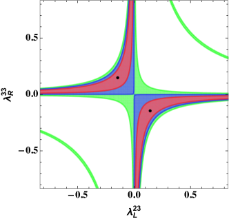
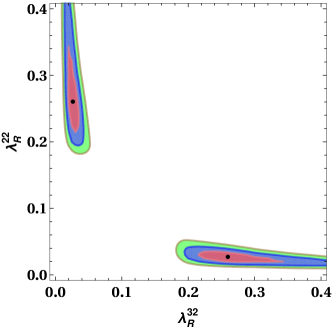
Figure 5: Constraints on new LQ couplings from observables mediated by $b\to c\tau\bar{\nu}$ (left panel) and $b\to s\mu^{+}\mu^{-}$ (right panel). Different colors correspond to $1\sigma$, $2\sigma$, and $3\sigma$ contours and the black dots represent the best-fit value.

Scenarios	Couplings	Best-fit Values	Pull
C-I	$(\lambda_{L}^{23},~{}{\lambda_{R}^{33}})$	$(-0.143,0.147)$	$3.5$
		$(0.147,-0.143)$
C-II	$(\lambda_{R}^{32},~{}{\lambda_{R}^{22}})$	$(0.0265,0.260)$	$5.4$
		$(0.260,0.0265)$

Table 6: . Best-fit values of new LQ couplings, and pull values for all cases (C-I, C-II).

V.4 Implications on lepton flavor violating $B$ and $\tau$ decays

In this section, we will discuss some of the lepton flavor violating (LFV) decay modes $B_{(s)}$ and $\Upsilon$ mesons as well as $\tau$ lepton, due to the impact of the scalar leptoquark, $R_{2}({\bf 3,2},7/6)$. The rare leptonic/semileptonic LFV decays of $B$ mesons involving the quark-level transitions $b\to s\ell_{i}^{+}\ell_{j}^{-}$, occur at tree level via the exchange of the SLQ. For illustration, in the left panel of Fig. 6, we show the Feynman diagram for $b\to s\tau\mu$ LFV process as a typical example. The effective Hamiltonian for $b\to s\ell_{i}^{+}\ell_{j}^{-}$ process due to the effect of scalar LQ can be given as Sahoo and Mohanta (2015, 2016)

$$\mathcal{H}_{\rm eff}\left(b\to s\ell_{i}^{+}\ell_{j}^{-}\right) \ =\ \Big{[}G_{V}\left(\bar{s}\gamma^{\mu}P_{L}b\right)\left(\bar{\ell}_{i}\gamma_{\mu}\ell_{j}\right)+G_{A}\left(\bar{s}\gamma^{\mu}P_{L}b\right)\left(\bar{\ell}_{i}\gamma_{\mu}\gamma_{5}\ell_{j}\right)\Big{]}\;,$$ (54)

where the vector and axial vector couplings $G_{V,A}$ are expressed as

$$G_{V}=G_{A}=\frac{\lambda_{R}^{j3}(\lambda_{R}^{i2})^{*}}{8m_{\rm LQ}^{2}}\;.$$ (55)

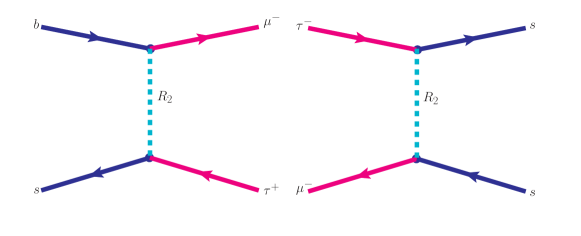
Figure 6: Feynman diagrams for the LFV processes $b\to s\tau^{+}\mu^{-}$ (left panel), and $\tau\to\mu\phi~{}(\eta^{(\prime)})$ (right panel) mediated through the exchange of scalar LQ.

This effective Hamiltonian leads to the following decay processes:

1. $\boldsymbol{B_{s}\to\ell_{i}^{+}\ell_{j}^{-}}$ : The branching ratio of the LFV decay process $B_{s}\to\ell_{i}^{+}\ell_{j}^{-}$, in the presence of scalar LQ is given as  Bečirević et al. (2016)

   $${\rm BR}(\overline{B}_{s}\to\ell_{i}^{-}\ell_{j}^{+})\ =\ \tau_{B_{s}}\frac{1}{8\pi M_{B_{s}}^{3}}|f_{B_{s}}G_{V}|^{2}\lambda^{1/2}(M_{B_{s}}^{2},m_{i}^{2},m_{j}^{2})$$

   $$\times\Bigg{[}(m_{j}-m_{i})^{2}\Big{(}M_{B_{s}}^{2}-(m_{i}+m_{j})^{2}\Big{)}+(m_{j}+m_{i})^{2}\Big{(}M_{B_{s}}^{2}-(m_{i}-m_{j})^{2}\Big{)}\Bigg{]},$$ (56)

   where $f_{B_{s}}$ represents the decay constant of $B_{s}$ and

   $$\lambda(a,b,c)\ =\ a^{2}+b^{2}+c^{2}-2\left(ab+bc+ac\right)\;,$$ (57)

   is the triangle function.

2. $\boldsymbol{\overline{B}\to\overline{K}\ell_{i}^{+}\ell_{j}^{-}}$ : The differential branching fraction of $B\to K\ell_{i}^{+}\ell_{j}^{-}$ process is given as Sahoo and Mohanta (2016)

   $$\frac{{\rm d}{\rm BR}}{{\rm d}q^{2}}(\overline{B}\to\overline{K}\ell_{i}^{+}\ell_{j}^{-})=2\tau_{B}\Big{(}a(q^{2})+\frac{1}{3}c(q^{2})\Big{)}\,,$$ (58)

   where the coefficients $a(q^{2})$ and $c(q^{2})$ are expressed as

   $$a(q^{2}) = \Gamma_{0}\frac{\sqrt{\lambda_{1}\lambda_{2}}}{q^{2}}f_{+}^{2}\Bigg{[}\left(|G_{V}|^{2}+|G_{A}|^{2}\right)\frac{\lambda_{1}}{4}+|G_{S}|^{2}\left(q^{2}-(m_{i}+m_{j})^{2}\right)$$ (59)

   $$+ |G_{P}|^{2}\left(q^{2}-(m_{i}-m_{j})^{2}\right)+|G_{A}|^{2}M_{B}^{2}(m_{i}+m_{j})^{2}+|G_{V}|^{2}M_{B}^{2}(m_{i}-m_{j})^{2}$$

   $$+ \left(M_{B}^{2}-M_{K}^{2}+q^{2}\right)\Big{(}(m_{i}+m_{j})Re(G_{P}G_{A}^{*})+(m_{j}-m_{i})Re(G_{S}G_{V}^{*})\Big{)}\Bigg{]}\;,$$

   $$c(q^{2})=-\Gamma_{0}f_{+}^{2}\frac{(\lambda_{1}\lambda_{2})^{3/2}}{4q^{6}}\left(|G_{A}|^{2}+|G_{V}|^{2}\right)\;,\hskip 170.71652pt$$ (60)

   with

   $$\Gamma_{0}=\frac{1}{2^{8}\pi^{3}M_{B}^{3}},\hskip 28.45274pt\lambda_{1}=\lambda(M_{B}^{2},M_{K}^{2},q^{2}),\hskip 28.45274pt\lambda_{2}=\lambda(q^{2},m_{i}^{2},m_{j}^{2})\;,$$ (61)

   and

   $$G_{S} = \frac{1}{2}G_{V}(m_{j}-m_{i})\Bigg{[}\frac{M_{B}^{2}-M_{K}^{2}}{q^{2}}\left(\frac{f_{0}(q^{2})}{f_{+}(q^{2})}-1\right)-1\Bigg{]}\;,$$

   $$G_{P} = \frac{1}{2}G_{A}(m_{i}+m_{j})\left[\frac{M_{B}^{2}-M_{K}^{2}}{q^{2}}\left(\frac{f_{0}(q^{2})}{f_{+}(q^{2})}-1\right)-1\right]\;.$$ (62)

   $f_{0,+}$ are the form factors describing $B\to K$ transitions.

3. $\boldsymbol{\overline{B}\to\overline{K}^{*}\ell_{i}^{+}\ell_{j}^{-}}$ and $\boldsymbol{\overline{B}_{s}\to\phi\ell_{i}^{+}\ell_{j}^{-}}$ : The differential branching fraction of $\overline{B}\to\overline{K}^{*}\ell_{i}^{+}\ell_{j}^{-}$ process is given as Sahoo and Mohanta (2016)

   $$\frac{\rm dBR}{dq^{2}} = \tau_{B}\Gamma_{V}\times\Bigg{[}A(q^{2})^{2}\Bigg{\{}\frac{2}{3}\lambda_{K^{*}}\left(1-\left(\frac{m_{i}^{2}}{q^{2}}\right)^{2}\right)+8M_{K^{*}}^{2}(q^{2}-m_{i}^{2})$$ (63)

   $$-\frac{2}{9}\left(1-\frac{m_{i}^{2}}{q^{2}}\right)^{2}\left(\left(M_{B}^{2}-M_{K^{*}}^{2}-q^{2}\right)^{2}+8q^{2}M_{K^{*}}^{2}\right)\Bigg{\}}$$

   $$+B(q^{2})^{2}\Bigg{\{}\frac{\lambda_{K^{*}}}{6}\left(M_{B}^{2}-M_{K^{*}}^{2}-q^{2}\right)^{2}\left(1-\left(\frac{m_{i}^{2}}{q^{2}}\right)^{2}\right)-\frac{\lambda_{K^{*}}^{2}}{18}\left(1-\frac{m_{i}^{2}}{q^{2}}\right)^{2}$$

   $$-\frac{2}{3}\lambda_{K^{*}}M_{K^{*}}^{2}(q^{2}-m_{i}^{2})\Bigg{\}}+C(q^{2})^{2}\Bigg{\{}\frac{2}{3}\lambda_{K^{*}}m_{i}^{2}(q^{2}-m_{i}^{2})\Bigg{\}}$$

   $$-D(q^{2})^{2}\Bigg{\{}\frac{4}{9}\lambda_{K^{*}}M_{K^{*}}^{2}(q^{2}-m_{i}^{2})\left(4-\frac{m_{i}^{2}}{q^{2}}\right)\Bigg{\}}$$

   $$-Re\Big{(}A(q^{2})B(q^{2})^{*}\Big{)}\Bigg{\{}\frac{2}{3}\lambda_{K^{*}}\left(M_{B}^{2}-M_{K^{*}}^{2}-q^{2}\right)\left(1-\left(\frac{m_{i}^{2}}{q^{2}}\right)^{2}-\frac{1}{3}\left(1-\frac{m_{i}^{2}}{q^{2}}\right)^{2}\right)\Bigg{\}}$$

   $$-Re\Big{(}A(q^{2})C(q^{2})^{*}\Big{)}\Bigg{\{}\frac{4}{3}\lambda_{K^{*}}m_{i}^{2}\left(1-\frac{m_{i}^{2}}{q^{2}}\right)\Bigg{\}}$$

   $$+Re\Big{(}B(q^{2})C(q^{2})^{*}\Big{)}\Bigg{\{}\frac{2}{3}\lambda_{K^{*}}m_{i}^{2}\left(M_{B}^{2}-M_{K^{*}}^{2}-q^{2}\right)\left(1-\frac{m_{i}^{2}}{q^{2}}\right)\Bigg{\}}\Bigg{]},$$

   where

   $$\Gamma_{V}=\frac{3\sqrt{\lambda_{K^{*}}}}{2^{11}M_{K^{*}}^{2}\left(\pi M_{B}\beta\right)^{3}}|G_{V}|^{2}\;,\hskip 14.22636pt\lambda_{K^{*}}=\lambda\left(M_{B}^{2},M_{K^{*}}^{2},q^{2}\right)\;,\hskip 14.22636pt\beta={1\over M_{K^{*}}^{2}}\lambda^{1/2}\left(M_{B}^{2},M_{K^{*}}^{2},q^{2}\right),$$

   and the functions $A(q^{2}),~{}B(q^{2}),~{}C(q^{2})$ and $D(q^{2})$ are related to the various form factors of $B\to K^{*}$ transitions as

   $$A(q^{2}) = \left(M_{B}+M_{K^{*}}\right)A_{1}(q^{2})\;,\hskip 79.6678ptB(q^{2})=\frac{2A_{2}(q^{2})}{\left(M_{B}+M_{K^{*}}\right)}\;,$$

   $$C(q^{2}) = \frac{A_{2}(q^{2})}{\left(M_{B}+M_{K^{*}}\right)}+\frac{2M_{K^{*}}}{q^{2}}\left(A_{3}(q^{2})-A_{0}(q^{2})\right)\;,\hskip 7.11317ptD(q^{2})=\frac{2V(q^{2})}{\left(M_{B}+M_{K^{*}}\right)}\;.\hskip 14.22636pt$$ (65)

   The same expression can be used for $B_{s}\to\phi\ell_{i}\ell_{j}$ processes by appropriately replacing the particle masses and the lifetime of $B_{s}$ meson. For numerical estimation, we use the particle masses and $B$ meson lifetimes as well as other input parameters from PDG Zyla et al. (2020) . Using $f_{B_{s}}=(225.6\pm 1.1\pm 5.4)$ MeV Charles et al. (2015) and best-fit values of the new couplings from Table 6, we present our predicted results on various branching ratios of LFV decays of $B$ mesons in Table 7 . It can be noticed from the table that the branching fractions of various LFV $B$ decays are quite significant in the presence of $R_{2}$ scalar leptoquark and are within the reach of Belle-II or LHCb experiments. However, for most of these decays, the experimental limits are not yet available. The LFV channels which have been searched for are $B^{+}\to K^{+}\mu^{-}\tau^{+}(\mu^{+}\tau^{-})$ Lees et al. (2012b) and $B_{s}\to\tau^{\pm}\mu^{\mp}$ Aaij et al. (2019b) for which we find our predicted branching fraction values are well below the present 90% CL upper limits. Our obtained result on ${\rm BR}(B_{s}\to\tau^{\pm}\mu^{\mp})$ is

   $${\rm BR}(B_{s}\to\tau^{\pm}\mu^{\mp})\ =\ {\rm BR}(B_{s}\to\tau^{+}\mu^{-})+{\rm BR}(B_{s}\to\tau^{-}\mu^{+})=1.3\times 10^{-9}\,,$$ (66)

   which is well below the current experimental limit at 90% C.L. Aaij et al. (2019b) ${\rm BR}(B_{s}\to\tau^{\pm}\mu^{\mp})^{\rm exp}\ <\ 3.4\times 10^{-5}\,.$ Our predicted branching ratios for the LFV processes $B_{(s)}\to(K,K^{*},\phi)\mu^{-}\tau^{+}(\mu^{+}\tau^{-})$ are quite reasonable and are within the reach of Belle-II Altmannshofer et al. (2019) as well as the upcoming LHCb upgrade Aaij et al. (2018c). In Fig. 7 , we display the differential branching fractions of the decay modes $B^{+}\to K^{+}\mu^{-}\tau^{+}$ (top-left panel), $B^{+}\to K^{*+}\mu^{-}\tau^{+}$ (top-right panel) and $B_{s}\to\phi\mu^{-}\tau^{+}$ (bottom panel) with respect to $q^{2}$.

   Decay modes	Predicted values	Experimental Limit
   $B_{s}\to\mu^{-}\tau^{+}$	$3.03\times 10^{-9}$	$<3.4\times 10^{-5}$ (90% CL) Aaij et al. (2019b)
   $B^{+}\to K^{+}\mu^{-}\tau^{+}$	$1.5\times 10^{-8}$	$<2.8\times 10^{-5}$ (90% CL) Lees et al. (2012b)
   $\overline{B}^{0}\to\overline{K}^{0}\mu^{-}\tau^{+}$	$1.4\times 10^{-8}$	$\cdots$
   $B^{+}\to K^{*+}\mu^{-}\tau^{+}$	$2.91\times 10^{-8}$	$\cdots$
   $\overline{B}^{0}\to\overline{K}^{*0}\mu^{-}\tau^{+}$	$2.7\times 10^{-8}$	$\cdots$
   $B_{s}\to\phi\mu^{-}\tau^{+}$	$3.5\times 10^{-8}$	$\cdots$
   $B_{s}\to\mu^{+}\tau^{-}$	$3.2\times 10^{-9}$	$<3.4\times 10^{-5}$ (90% CL) Aaij et al. (2019b)
   $B^{+}\to K^{+}\mu^{+}\tau^{-}$	$1.6\times 10^{-8}$	$<4.5\times 10^{-5}$ (90% CL) Lees et al. (2012b)
   $\overline{B}^{0}\to\overline{K}^{0}\mu^{+}\tau^{-}$	$1.5\times 10^{-8}$	$\cdots$
   $B^{+}\to K^{*+}\mu^{+}\tau^{-}$	$3.1\times 10^{-8}$	$\cdots$
   $\overline{B}^{0}\to\overline{K}^{*0}\mu^{+}\tau^{-}$	$2.8\times 10^{-8}$	$\cdots$
   $B_{s}\to\phi\mu^{+}\tau^{-}$	$3.7\times 10^{-8}$	$\cdots$
   $\Upsilon(1S)\to\mu^{\mp}\tau^{\pm}$	$2.12\times 10^{-12}$	$6.0\times 10^{-6}~{}(95\%~{}{\rm CL})$ Zyla et al. (2020)
   $\Upsilon(2S)\to\mu^{\mp}\tau^{\pm}$	$2.16\times 10^{-12}$	$3.3\times 10^{-6}~{}(90\%~{}{\rm CL})$ Zyla et al. (2020)
   $\Upsilon(3S)\to\mu^{\mp}\tau^{\pm}$	$2.82\times 10^{-12}$	$3.1\times 10^{-6}~{}(90\%~{}{\rm CL})$ Zyla et al. (2020)
   $\tau^{-}\to\mu^{-}\phi$	$4.4\times 10^{-10}$	$<8.4\times 10^{-8}$ (90% CL) Miyazaki et al. (2011)
   $\tau^{-}\to\mu^{-}\eta$	$2.18\times 10^{-10}$	$<6.5\times 10^{-8}$ (90% CL) Zyla et al. (2020)
   $\tau^{-}\to\mu^{-}\eta^{\prime}$	$5.49\times 10^{-10}$	$<1.3\times 10^{-7}$ (90% CL) Zyla et al. (2020)

   Table 7: Predicted values of the branching ratios of lepton flavor violating decay channels of $B$ meson and $\tau$ lepton in the present model.

   

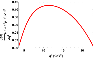
   (a)  $B^{+}\to K^{+}\mu^{-}\tau^{+}$

   

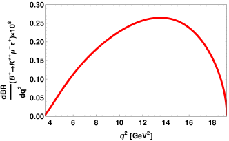
   (b)  $B^{+}\to K^{*+}\mu^{-}\tau^{+}$

   

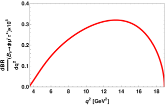
   (c)  $B_{s}\to\phi\mu^{-}\tau^{+}$

   Figure 7: Behaviour of the differential branching fractions of the LFV processes (a) $B^{+}\to K^{+}\mu^{-}\tau^{+}$, (b)$B^{+}\to K^{*+}\mu^{-}\tau^{+}$ and (c) $B_{s}\to\phi\mu^{-}\tau^{+}$ with respect to $q^{2}$ due to the effect of $R_{2}^{3/2}$ leptoquark.

4. ${\boldsymbol{\Upsilon(nS)\to\mu\tau}}$ : The LFV process $\Upsilon(nS)\to\mu\tau$ can occur at tree level in the LQ model and the corresponding Feynman diagram can be obtained from that of $b\to s\mu\tau$ process (left panel of Fig. 6) by replacing $s\to b$, and the branching ratio for this process is given as Bhattacharya et al. (2017)

   $${\rm BR}(\Upsilon(nS)\to\mu^{-}\tau^{+})\ = \ \frac{f_{\Upsilon(nS)}^{2}m_{\Upsilon(nS)}^{3}}{48\pi\Gamma_{\Upsilon(nS)}}\left(2-\frac{m_{\tau}^{2}}{m_{\Upsilon(nS)}^{2}}-\frac{m_{\tau}^{4}}{m_{\Upsilon(nS)}^{4}}\right)\left(1-\frac{m_{\tau}^{2}}{m_{\Upsilon(nS)}^{2}}\right)\left|\frac{\lambda_{R}^{32}\lambda_{R}^{33*}}{8m_{{\rm LQ}}^{2}}\right|^{2}\,.$$

   The branching ratio for the process $\Upsilon(nS)\to\mu^{+}\tau^{-}$ can be obtained from ${\rm BR}(\Upsilon(nS)\to\mu^{-}\tau^{+})$ by appropriately replacing the LQ couplings, i.e., $\lambda_{R}^{32}\lambda_{R}^{33*}\to\lambda_{R}^{33}\lambda_{R}^{32*}$. Hence, the branching ratio for $\Upsilon(nS)\to\mu^{\mp}\tau^{\pm}$ process is given as

   $${\rm BR}(\Upsilon(nS)\to\mu^{\mp}\tau^{\pm})={\rm BR}(\Upsilon(nS)\to\mu^{-}\tau^{+})+{\rm BR}(\Upsilon(nS)\to\mu^{+}\tau^{-})\,.$$ (68)

   For numerical estimation, all the particle masses and widths of $\Upsilon(nS),~{}n=1,2,3$ are taken from PDG Zyla et al. (2020) . The values of $\Upsilon(nS)$ decay constants used are as follows: $f_{\Upsilon(1S)}=(700\pm 16)$ MeV, $f_{\Upsilon(2S)}=(496\pm 21)$ MeV and $f_{\Upsilon(3S)}=(430\pm 21)$ MeV Bhattacharya et al. (2017) . With these input parameters the predicted branching ratios of $\Upsilon(nS)\to\mu^{\pm}\tau^{\mp}$ are provided in Table 7 , which are far below the current experimental upper limits Zyla et al. (2020).

5. ${\boldsymbol{\tau\to\mu\phi}}$ : The Feynman diagram for the LFV decay process $\tau\to\mu\phi$ is presented in the right panel of Fig. 6 and its branching ratio is expressed as Bečirević et al. (2016)

   $${\rm BR}(\tau\to\mu\phi)\ =\ \frac{\tau_{\tau}f_{\phi}^{2}m_{\phi}^{4}}{256\pi m_{\tau}^{3}}\left|\frac{\lambda_{R}^{23}\lambda_{R}^{22*}}{m_{{\rm LQ}}^{2}}\right|^{2}\times\lambda^{1/2}(m_{\phi}^{2},m_{\tau}^{2},m_{\mu}^{2})\left[-1+\frac{(m_{\mu}^{2}+m_{\tau}^{2})}{2m_{\phi}^{2}}+\frac{(m_{\mu}^{2}-m_{\tau}^{2})^{2}}{2m_{\phi}^{4}}\right],$$

   where $f_{\phi}$ is the $\phi$ meson decay constant. Using $f_{\phi}=(238\pm 3)$ MeV from Ref. Chakraborty et al. (2017), and the other input parameters from PDG Zyla et al. (2020), along with the best-fit values of required new parameters from Table 6 , the predicted branching fraction of $\tau\to\mu\phi$ is shown in Table 7 . We find that the branching ratio is substantially enhanced and is within the reach of Belle-II experiment.

6. ${\boldsymbol{\tau\to\mu\eta^{(\prime)}}}$ : The branching ratio for $\tau\to\mu\eta^{(\prime)}$ process is given as

   $${\rm BR}(\tau\to\mu\eta^{(\prime)})\ = \ \frac{\tau_{\tau}f_{\eta^{(\prime)}}^{2}m_{\tau}^{3}}{512\pi}\left|\frac{\lambda_{R}^{23}\lambda_{R}^{22*}}{m_{{\rm LQ}}^{2}}\right|^{2}\left(1-\frac{m_{\eta^{(\prime)}}^{2}}{m_{\tau}^{2}}\right)^{2}\,.$$ (70)

   Using $f_{\eta}\simeq-157.63$ MeV, Bhattacharya et al. (2017), $f_{\eta^{\prime}}\simeq 31.76$ MeV Bhattacharya et al. (2017), along with other input parameters from Zyla et al. (2020) and the best-fit values of LQ couplings from Table 6 , our predicted values of branching ratios of $\tau\to\mu\eta^{(\prime)}$ processes are presented in Table 7 , which are found to be substantially lower than the current experimental upper limits.

VI Dark Matter

We consider fermion triplet $\Sigma(1,3,0)$ coming from the fermion representation $45_{F}$ of $SO(10)$. The stability of fermion triplet dark matter is ensured from the matter parity under which $16_{F}$ is odd while $45_{F}$ is even. SM Higgs is contained in $10_{S}$ and the scalar leptoquark $R_{2}$ is contained in $126_{S}$, are both even under matter parity Hambye (2011). The generic Yukawa term $y\Sigma\bar{\ell_{L}}\phi$ mediating neutrino masses by type-III seesaw is not allowed, which can be understood as follows. The SM lepton doublet is contained in $16_{F}$, scalar doublet resides in $10_{S}$, while the fermion triplet DM exists in $45_{F}$ and the Lagrangian term in $SO(10)$ bilinear $16_{F}10_{H}45_{F}$ is actually forbidden because of the matter parity. Hence the fermion triplet mass comes from the invariant bilinear $M_{\Sigma}45_{F}45_{F}$ and the relic density of DM is solely controlled by the gauge interactions. The low energy invariant interaction term for fermion triplet DM is given by

$$\mathcal{L}_{\rm\Sigma} =\frac{i}{2}{\rm Tr}[\overline{\Sigma_{R}}\not{D}\Sigma_{R}]+\frac{i}{2}{\rm Tr}[\overline{\Sigma^{c}_{R}}\not{D}\Sigma^{c}_{R}]-\left(\frac{1}{2}{\rm Tr}[\overline{\Sigma^{c}_{R}}M_{\Sigma}\Sigma_{R}]+{\rm h.c.}\right),$$ (71)

where, $\Sigma^{c}_{R}=C\overline{\Sigma_{R}}^{T}$ is the CP conjugate of $\Sigma_{R}$ with $C$ being the operator for charge conjugation and $D_{\mu}$ is the covariant derivative for $\Sigma_{R}$, given by

$$D_{\mu}=\partial_{\mu}\Sigma_{R}+ig\left[\sum_{a=1}^{3}\frac{\sigma^{a}}{2}W^{a}_{\mu},\Sigma_{R}\right].$$ (72)

Defining the four component Dirac spinor as $\psi^{-}=\Sigma^{-}_{R}+\Sigma^{+c}_{R}$ and Majorana fermion as $\psi^{0}=\Sigma^{0}_{R}+\Sigma^{0c}_{R}$, we write the Lagrangian for fermion triplet as Biswas et al. (2018)

$$\mathcal{L}_{\rm triplet} =\overline{\psi^{-}}i\not{\partial}\psi^{-}+\frac{1}{2}\overline{\psi^{0}}i\not{\partial}\psi^{0}-M_{\psi^{-}}\overline{\psi^{-}}\psi^{-}-\frac{M_{\psi^{0}}}{2}\overline{\psi^{0}}\psi^{0}$$ (73)

$$+g\left(\cos\theta_{w}\overline{\psi^{-}}\gamma_{\mu}\psi^{-}Z^{\mu}+\sin\theta_{w}\overline{\psi^{-}}\gamma_{\mu}\psi^{-}A^{\mu}\right)$$

$$-g\left(\overline{\psi^{-}}\gamma^{\mu}\psi^{0}W_{\mu}^{-}+{\rm h.c.}\right).$$

VI.1 Relic abundance

The neutral component of fermion triplet ($\psi^{0}$) is Majorana type and the charged component ($\psi^{\pm}$) is Dirac in nature. At tree-level, both the charged and neutral components remain degenerate in mass. However, one-loop electroweak radiative corrections provide a mass splitting of $\delta=166$ MeV Cirelli et al. (2006); Ma and Suematsu (2009), where $\delta=M_{\psi^{\pm}}-M_{\psi^{0}}$. Thus the Majorana fermion $\psi^{0}$ is the lightest thermal dark matter candidate in the present model and its relic density is governed by the gauge interactions 73. We have used the packages LanHEP Semenov (1996) and micrOMEGAs Pukhov et al. (1999); Belanger et al. (2007, 2009) to extract compute dark matter relic density. With the mentioned mass splitting, co-annihilation’s also contribute to dictate relic density in addition to annihilation’s. The processes include $\psi^{0}\overline{\psi^{0}}\to W^{+}W^{-}$ (via t-channel $\psi^{-}$ exchange), $\psi^{\pm}\psi^{\pm}\to W^{\pm}W^{\pm}$ (via t-channel $\psi^{0}$ exchange), $\psi^{+}\psi^{-}\to f\overline{f}$ (via s-channel $A,Z$ exchange) with $f=u,d,s,c,t,b,e,\mu,\tau$ and $\psi^{0}\psi^{-}\to\overline{f^{\prime}},f^{\prime\prime}$ (via s-channel $W^{-}$ exchange) with $f^{\prime}=u,c,t,\nu_{e},\nu_{\mu},\nu_{\tau}$ and $f^{\prime\prime}=d,s,c,e,\mu,\tau$. Fig. 8 depicts the relic density as a function of DM mass, with contribution from the above mentioned channels. The abundance meets the Planck limit ($3\sigma$) Aghanim et al. (2018) in the mass region $2.34$ TeV to $2.4$ TeV Ma and Suematsu (2009); Biswas et al. (2018).

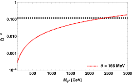
Figure 8: Relic abundance as a function of DM mass with contributions from annihilation’s and co-annihilation’s of $\psi^{0}$ and $\psi_{\pm}$. Black horizontal dashed lines correspond to $3\sigma$ region of Planck satellite data.

VI.2 Direct searches

Moving on to the detection perspective, the neutral component $\psi^{0}$ can produce a nuclear recoil through Higgs penguin and box diagram with W loop Cai and Spray (2016). The effective interaction is given by

$$\mathcal{L}=\sum_{i}\xi^{i}_{q}\overline{\psi^{0}}\psi^{0}\overline{q_{i}}q_{i}.$$ (74)

Here,

$$\xi^{i}_{q} = -\alpha^{2}_{2}\frac{m_{q_{i}}}{M_{\psi^{0}}}\bigg{[}-\frac{1-4n_{W}+3n_{W}^{2}-(4n_{W}-2){\rm log}~{}n_{W}}{m_{h}^{2}(1-n_{W})^{3}}$$

$$+\frac{2-3n_{W}+6n_{W}^{2}-5n_{W}^{3}+3n_{W}(1+n_{W}^{2}){\rm log}~{}n_{W}}{6m_{W}^{2}(1-n_{W})^{4}}\bigg{]},$$

with $n_{W}=m_{W}^{2}/m^{2}_{\psi^{0}}$ and $\alpha_{2}=\frac{g^{2}}{4\pi}$. Thus, the spin-independent (SI) cross section is given by

$$\sigma^{\rm loop}_{\rm SI}=\frac{4~{}\mu_{r}^{2}}{\pi}m^{2}_{p}\left(\frac{\xi^{i}_{q}}{m_{q_{i}}}\right)^{2}f_{p}^{2},$$ (76)

where, $m_{p}$ is proton mass, $\mu_{r}$ is the reduced mass of DM-nucleon system and $f_{p}\simeq 0.3$. Figure. 9 projects the SI Cross section as a function of DM mass. We notice that the loop contribution is well below the upper limits levied by PandaX-II Cui et al. (2017), XENON1T Aprile et al. (2017) and LUX Akerib et al. (2017).

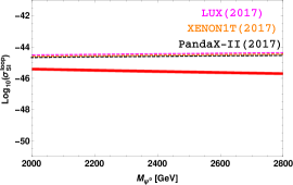
Figure 9: One-loop SI contribution projected with the stringent upper limits of PandaX-II Cui et al. (2017), XENON1T Aprile et al. (2017) and LUX Akerib et al. (2017).

In case of indirect searches, DM can provide gamma ray signal via $W^{\pm}$ at loop level. However, Fermi-LAT with Sommerfeld enhancement rules out such suppressed cross section from a TeV scale DM Bern et al. (1997); Choubey et al. (2018).

VII Conclusion

We have considered an extension of standard model by a scalar leptoquark $R_{2}$ and a fermion triplet $\Sigma$ and embedded the framework in non-SUSY $SO(10)$ GUT. The introduction of $R_{2}$ and $\Sigma$ at few TeV scale assist the unification of gauge couplings of strong and electroweak forces while consistent with flavor anomalies $R_{K}$, $R_{K^{(*)}}$, $R_{D^{(*)}}$, $R_{J/\psi}$ and dark matter phenomenology.

The right-handed neutrino which is part of $16_{F}$ spinorial representation of $SO(10)$ can explain the non-zero neutrino masses. The dark matter comes from $45_{F}$ of $SO(10)$, while the scalar leptoquark is contained in the $126_{S}$. Since $16_{F}$ is odd while all other multiplets are even under matter parity $P_{M}$ and thus ensure the stability of fermion triplet dark matter.

The unification mass scale comes out to be $M_{U}=10^{13.27}\,\,\mbox{GeV}$ which is well below the limit set by the proton decay experiments. In order to satisfy experimental bound on proton decay, we adopt one loop GUT threshold corrections arising due to presence of super heavy scalars, fermions and gauge bosons by modifying the one-loop beta coefficients and revolution of gauge couplings at the GUT scale $M_{U}$. After including threshold corrections, the modified value of unification mass scale is found to be $10^{16.323}$, which resulted the proton life time as $\tau_{p}=7.7\times 10^{36}$ years.

The proposed model incorporates the scalar leptoquark $R_{2}(3,2,7/6)$, which plays a crucial role in explaining the recently observed flavor anomalies in semileptonic $B$ decays. The intriguing feature of this leptoquark is that, it can induce additional contributions to the CC $b\to c\tau\bar{\nu}_{\tau}$ as well as NC $b\to s\ell^{+}\ell^{-}$ transitions at the tree level due to the exchange of LQ and hence, can successfully account for the observed discrepancies in the LFU violating observables. In this work, the leptoquark couplings are constrained by using the LFU observables $R_{D^{(*)}}$, $R_{J/\psi}$, ${\rm BR}(B_{c}\to\tau\bar{\nu}_{\tau})$ for $b\to c\tau\bar{\nu}_{\tau}$ transitions and $R_{K^{(*)}}$, ${\rm BR}(B_{s}\to\mu^{+}\mu^{-})$, and various observables of $B\to K^{*}\mu^{+}\mu^{-}$ and $B_{s}\to\phi\mu^{+}\mu^{-}$ processes for $b\to s\ell\ell$ transitions for the representative mass of LQ as $m_{\rm LQ}=1.2$ TeV. Using these constrained couplings, we have predicted the branching ratios of various LFV decays of $B$ and $B_{s}$ mesons such as $B\to K^{(*)}\ell_{i}^{+}\ell_{j}^{-}$, $B_{s}\to\phi\ell_{i}^{+}\ell_{j}^{-}$ and $B_{s}\to\ell_{i}^{+}\ell_{j}^{-}$. We found that the branching fractions of these decay modes are substantially enhanced due to the effect of $R_{2}$ SLQ and are within the reach of the Belle-II and LHCb experiments. The observation of these decay modes provide an indirect hint for the existence of the SLQ $R_{2}(3,2,7/6)$. In addition, we have also investigated the LFV decays $\Upsilon\to\mu^{\pm}\tau^{\mp}$, $\tau\to\mu^{-}\phi$ and $\tau\to\mu^{-}\eta(\eta^{\prime})$. Furthermore, the neutral component of fermion triplet $\Sigma$ contributes to the relic abundance of the Universe near $2.34$ to $2.4$ TeV mass regime. One loop spin-independent DM-nucleon cross section is also suitably obtained within upper limits of experiments such as XNENON1T, LUX and PandaX-II.

Appendix A One loop GUT Threshold corrections to SM gauge couplings

The analytical relation for the threshold corrections at $M_{GUT}$ in the $G_{SM}$ model,are

$$\boldsymbol{\lambda^{U}_{3C}}=5 -21\bigg{[}\eta_{V_{4}}+\eta_{V_{5}}+\eta_{V_{6}}+\eta_{V_{7}}+\frac{1}{2}\eta_{V_{8}}+\frac{1}{2}\eta_{V_{9}}\bigg{]}$$

$$+2\bigg{[}\frac{1}{2}\eta_{S_{2}}+\frac{1}{2}\eta_{S_{3}}+\eta_{S_{4}}+\frac{1}{2}\eta_{S_{5}}+\frac{15}{2}\eta_{S_{7}}+\frac{1}{2}\eta_{S_{11}}+\frac{1}{2}\eta_{S_{12}}+\frac{5}{2}\eta_{S_{13}}+\frac{5}{2}\eta_{S_{14}}$$

$$+\frac{5}{2}\eta_{S_{15}}+\eta_{S_{18}}+\eta_{S_{19}}+\eta_{S_{20}}+6\eta_{S_{21}}+6\eta_{S_{22}}+\frac{3}{2}\eta_{S_{23}}\bigg{]}$$

$$+8\big{[}\eta_{F_{4}}+\eta_{F_{5}}+\eta_{F_{6}}+\eta_{F_{7}}+\frac{1}{2}\eta_{F_{8}}+\frac{1}{2}\eta_{F_{9}}+3\eta_{F_{10}}\big{]}$$ (77)

$$\boldsymbol{\lambda^{U}_{2L}}=6 -21\bigg{[}\frac{3}{2}\eta_{V_{4}}+\frac{3}{2}\eta_{V_{5}}+\frac{3}{2}\eta_{V_{6}}+\frac{3}{2}\eta_{V_{7}}\bigg{]}$$

$$+2\bigg{[}\frac{1}{2}\eta_{S_{1}}+2\eta_{S_{6}}+12\eta_{S_{7}}+\frac{1}{2}\eta_{S_{16}}+\frac{1}{2}\eta_{S_{17}}+\frac{3}{2}\eta_{S_{18}}+\frac{3}{2}\eta_{S_{19}}+\frac{3}{2}\eta_{S_{20}}+4\eta_{S_{21}}+4\eta_{S_{22}}+6\eta_{S_{23}}\bigg{]}$$

$$+8\big{[}\frac{3}{2}\eta_{F_{4}}+\frac{3}{2}\eta_{F_{5}}+\frac{3}{2}\eta_{F_{6}}+\frac{3}{2}\eta_{F_{7}}\big{]}$$ (78)

$$\boldsymbol{\lambda^{U}_{Y}}=8 -21\bigg{[}\frac{3}{5}\eta_{V_{1}}+\frac{3}{5}\eta_{V_{3}}+\frac{1}{10}\eta_{V_{4}}+\frac{5}{2}\eta_{V_{5}}+\frac{5}{2}\eta_{V_{6}}+\frac{1}{10}\eta_{V_{7}}+\frac{4}{5}\eta_{V_{8}}+\frac{4}{5}\eta_{V_{9}}\bigg{]}$$

$$+2\bigg{[}\frac{3}{10}\eta_{S_{1}}+\frac{1}{5}\eta_{S_{2}}+\frac{1}{5}\eta_{S_{3}}+\frac{2}{5}\eta_{S_{4}}+\frac{1}{5}\eta_{S_{5}}+\frac{9}{5}\eta_{S_{6}}+\frac{6}{5}\eta_{S_{7}}+\frac{3}{5}\eta_{S_{9}}+\frac{12}{5}\eta_{S_{10}}$$

$$+\frac{4}{5}\eta_{S_{11}}+\frac{16}{5}\eta_{S_{12}}+\frac{32}{5}\eta_{S_{13}}+\frac{2}{5}\eta_{S_{14}}+\frac{8}{5}\eta_{S_{15}}+\frac{3}{10}\eta_{S_{16}}+\frac{3}{10}\eta_{S_{17}}+\frac{1}{10}\eta_{S_{18}}$$

$$+\frac{49}{10}\eta_{S_{19}}+\frac{1}{10}\eta_{S_{20}}+\frac{12}{5}\eta_{S_{21}}+\frac{12}{5}\eta_{S_{22}}+\frac{3}{5}\eta_{S_{23}}\bigg{]}$$

$$+8\bigg{[}\frac{3}{5}\eta_{F_{1}}+\frac{3}{5}\eta_{F_{3}}+\frac{1}{10}\eta_{F_{4}}+\frac{5}{2}\eta_{F_{5}}+\frac{5}{2}\eta_{F_{6}}+\frac{1}{10}\eta_{F_{7}}+\frac{4}{5}\eta_{F_{8}}+\frac{4}{5}\eta_{F_{9}}\bigg{]}$$ (79)

References

- Bilenky (1999) S. M. Bilenky, in 1999 European School of High-Energy Physics (1999), pp. 187–217, eprint hep-ph/0001311.
- Mohapatra and Senjanovic (1980) R. N. Mohapatra and G. Senjanovic, Phys. Rev. Lett. 44, 912 (1980).
- Schechter and Valle (1980) J. Schechter and J. W. F. Valle, Phys. Rev. D 22, 2227 (1980).
- Babu and Mohapatra (1993) K. Babu and R. Mohapatra, Phys. Rev. Lett. 70, 2845 (1993), eprint hep-ph/9209215.
- Hosaka et al. (2006) J. Hosaka et al. (Super-Kamiokande), Phys. Rev. D 73, 112001 (2006), eprint hep-ex/0508053.
- Ahmad et al. (2002) Q. R. Ahmad et al. (SNO), Phys. Rev. Lett. 89, 011301 (2002), eprint nucl-ex/0204008.
- Abe et al. (2016) K. Abe et al. (Super-Kamiokande), Phys. Rev. D 94, 052010 (2016), eprint 1606.07538.
- Abe et al. (2019) K. Abe et al. (T2K), Phys. Rev. D 99, 071103 (2019), eprint 1902.06529.
- An et al. (2012) F. P. An et al. (Daya Bay), Phys. Rev. Lett. 108, 171803 (2012), eprint 1203.1669.
- Abe et al. (2012) Y. Abe et al. (Double Chooz), Phys. Rev. Lett. 108, 131801 (2012), eprint 1112.6353.
- Zwicky (1937) F. Zwicky, Astrophys. J. 86, 217 (1937).
- Zwicky (1933) F. Zwicky, Phys. Rev. 43, 147 (1933), URL https://link.aps.org/doi/10.1103/PhysRev.43.147.
- Bertone et al. (2005) G. Bertone, D. Hooper, and J. Silk, Phys. Rept. 405, 279 (2005), eprint hep-ph/0404175.
- Mambrini et al. (2015) Y. Mambrini, N. Nagata, K. A. Olive, J. Quevillon, and J. Zheng, Phys. Rev. D 91, 095010 (2015), eprint 1502.06929.
- Sakharov (1991) A. Sakharov, Sov. Phys. Usp. 34, 392 (1991).
- Kolb and Wolfram (1980) E. W. Kolb and S. Wolfram, Nucl. Phys. B 172, 224 (1980), [Erratum: Nucl.Phys.B 195, 542 (1982)].
- Fukugita and Yanagida (1986) M. Fukugita and T. Yanagida, Phys. Lett. B 174, 45 (1986).
- Fritzsch and Minkowski (1975) H. Fritzsch and P. Minkowski, Annals Phys. 93, 193 (1975).
- Bifani et al. (2019) S. Bifani, S. Descotes-Genon, A. Romero Vidal, and M.-H. Schune, J. Phys. G 46, 023001 (2019), eprint 1809.06229.
- Aaij et al. (2014a) R. Aaij et al. (LHCb), Phys. Rev. Lett. 113, 151601 (2014a), eprint 1406.6482.
- Aaij et al. (2019a) R. Aaij et al. (LHCb), Phys. Rev. Lett. 122, 191801 (2019a), eprint 1903.09252.
- Aaij et al. (2021) R. Aaij et al. (LHCb) (2021), eprint 2103.11769.
- Bobeth et al. (2007) C. Bobeth, G. Hiller, and G. Piranishvili, JHEP 12, 040 (2007), eprint 0709.4174.
- Bordone et al. (2016) M. Bordone, G. Isidori, and A. Pattori, Eur. Phys. J. C76, 440 (2016), eprint 1605.07633.
- Aaij et al. (2017) R. Aaij et al. (LHCb), JHEP 08, 055 (2017), eprint 1705.05802.
- Capdevila et al. (2018) B. Capdevila, A. Crivellin, S. Descotes-Genon, J. Matias, and J. Virto, JHEP 01, 093 (2018), eprint 1704.05340.
- Amhis et al. (2021) Y. S. Amhis et al. (HFLAV), Eur. Phys. J. C 81, 226 (2021), eprint 1909.12524.
- Na et al. (2015) H. Na, C. M. Bouchard, G. P. Lepage, C. Monahan, and J. Shigemitsu (HPQCD), Phys. Rev. D 92, 054510 (2015), [Erratum: Phys.Rev.D 93, 119906 (2016)], eprint 1505.03925.
- Fajfer et al. (2012a) S. Fajfer, J. F. Kamenik, and I. Nisandzic, Phys. Rev. D85, 094025 (2012a), eprint 1203.2654.
- Fajfer et al. (2012b) S. Fajfer, J. F. Kamenik, I. Nisandzic, and J. Zupan, Phys. Rev. Lett. 109, 161801 (2012b), eprint 1206.1872.
- Aaij et al. (2018a) R. Aaij et al. (LHCb), Phys. Rev. Lett. 120, 121801 (2018a), eprint 1711.05623.
- Wang et al. (2013) W.-F. Wang, Y.-Y. Fan, and Z.-J. Xiao, Chin. Phys. C37, 093102 (2013), eprint 1212.5903.
- Ivanov et al. (2005) M. A. Ivanov, J. G. Korner, and P. Santorelli, Phys. Rev. D71, 094006 (2005), [Erratum: Phys. Rev.D75,019901(2007)], eprint hep-ph/0501051.
- Abdesselam et al. (2021) A. Abdesselam et al. (Belle), JHEP 03, 105 (2021), eprint 1908.01848.
- Abdesselam et al. (2019a) A. Abdesselam et al. (Belle) (2019a), eprint 1904.02440.
- Aaij et al. (2013a) R. Aaij et al. (LHCb), Phys. Rev. Lett. 111, 191801 (2013a), eprint 1308.1707.
- Aaij et al. (2016) R. Aaij et al. (LHCb), JHEP 02, 104 (2016), eprint 1512.04442.
- Abdesselam et al. (2016a) A. Abdesselam et al. (Belle), in LHC Ski 2016: A First Discussion of 13 TeV Results (2016a), eprint 1604.04042.
- Aaij et al. (2014b) R. Aaij et al. (LHCb), JHEP 06, 133 (2014b), eprint 1403.8044.
- Aaij et al. (2013b) R. Aaij et al. (LHCb), JHEP 07, 084 (2013b), eprint 1305.2168.
- Georgi and Glashow (1974) H. Georgi and S. L. Glashow, Phys. Rev. Lett. 32, 438 (1974).
- Pati and Salam (1974) J. C. Pati and A. Salam, Phys. Rev. D10, 275 (1974), [Erratum: Phys. Rev.D11,703(1975)].
- Lavoura and Wolfenstein (1993) L. Lavoura and L. Wolfenstein, Phys. Rev. D 48, 264 (1993), URL https://link.aps.org/doi/10.1103/PhysRevD.48.264.
- Senjanović and Mohapatra (1975) G. Senjanović and R. N. Mohapatra, Phys.Rev. D12, 1502 (1975).
- Clark et al. (1982) T. E. Clark, T.-K. Kuo, and N. Nakagawa, Phys. Lett. 115B, 26 (1982).
- Altarelli and Meloni (2013a) G. Altarelli and D. Meloni, JHEP 08, 021 (2013a), eprint 1305.1001.
- Dueck and Rodejohann (2013a) A. Dueck and W. Rodejohann, JHEP 09, 024 (2013a), eprint 1306.4468.
- Meloni et al. (2014) D. Meloni, T. Ohlsson, and S. Riad, JHEP 12, 052 (2014), eprint 1409.3730.
- Meloni et al. (2017) D. Meloni, T. Ohlsson, and S. Riad, JHEP 03, 045 (2017), eprint 1612.07973.
- Preda et al. (2022) A. Preda, G. Senjanovic, and M. Zantedeschi (2022), eprint 2201.02785.
- Chakrabortty et al. (2018) J. Chakrabortty, R. Maji, S. K. Patra, T. Srivastava, and S. Mohanty, Phys. Rev. D 97, 095010 (2018), eprint 1711.11391.
- Bandyopadhyay and Raychaudhuri (2017) T. Bandyopadhyay and A. Raychaudhuri, Phys. Lett. B 771, 206 (2017), eprint 1703.08125.
- Gursey et al. (1976) F. Gursey, P. Ramond, and P. Sikivie, Phys. Lett. 60B, 177 (1976).
- Shafi (1978) Q. Shafi, Phys. Lett. B 79, 301 (1978).
- Nandi and Sarkar (1986) S. Nandi and U. Sarkar, Phys. Rev. Lett. 56, 564 (1986).
- Stech and Tavartkiladze (2004) B. Stech and Z. Tavartkiladze, Phys. Rev. D 70, 035002 (2004), eprint hep-ph/0311161.
- Huang (2014) C.-S. Huang, Mod. Phys. Lett. A 29, 1450150 (2014), eprint 1402.2737.
- Dash et al. (2021a) C. Dash, S. Mishra, S. Patra, and P. Sahu, Nucl. Phys. B 962, 115239 (2021a), eprint 2004.14188.
- Dash et al. (2020) C. Dash, S. Mishra, and S. Patra, Phys. Rev. D 101, 5 (2020), eprint 1911.11528.
- Dash et al. (2021b) C. Dash, S. Mishra, S. Patra, and P. Sahu (2021b), eprint 2109.12536.
- Bandyopadhyay and Maji (2019) T. Bandyopadhyay and R. Maji (2019), eprint 1911.13298.
- Mohapatra (1992) R. N. Mohapatra, Phys. Lett. B 285, 235 (1992).
- Hall (1981) L. J. Hall, Nucl. Phys. B178, 75 (1981).
- Babu and Khan (2015) K. Babu and S. Khan, Phys. Rev. D 92, 075018 (2015), eprint 1507.06712.
- Parida et al. (2017) M. Parida, B. P. Nayak, R. Satpathy, and R. L. Awasthi, JHEP 04, 075 (2017), eprint 1608.03956.
- Schwichtenberg (2019) J. Schwichtenberg, Eur. Phys. J. C 79, 351 (2019), eprint 1808.10329.
- Chakrabortty et al. (2019) J. Chakrabortty, R. Maji, and S. F. King, Phys. Rev. D 99, 095008 (2019), eprint 1901.05867.
- FUKUYAMA (2013) T. FUKUYAMA, International Journal of Modern Physics A 28, 1330008 (2013), ISSN 1793-656X, URL http://dx.doi.org/10.1142/S0217751X13300081.
- Frigerio et al. (2011) M. Frigerio, J. Serra, and A. Varagnolo, JHEP 06, 029 (2011), eprint 1103.2997.
- Alonso et al. (2014) R. Alonso, H.-M. Chang, E. E. Jenkins, A. V. Manohar, and B. Shotwell, Phys. Lett. B 734, 302 (2014), eprint 1405.0486.
- Dorsner et al. (2011) I. Dorsner, J. Drobnak, S. Fajfer, J. F. Kamenik, and N. Kosnik, JHEP 11, 002 (2011), eprint 1107.5393.
- Chang et al. (1985) D. Chang, R. N. Mohapatra, J. Gipson, R. E. Marshak, and M. K. Parida, Phys. Rev. D 31, 1718 (1985).
- Bertolini et al. (2009a) S. Bertolini, L. Di Luzio, and M. Malinský, Physical Review D 80 (2009a), ISSN 1550-2368, URL http://dx.doi.org/10.1103/PhysRevD.80.015013.
- Pati and Salam (1973) J. C. Pati and A. Salam, Phys. Rev. D 8, 1240 (1973).
- Minkowski (2015) P. Minkowski, Int. J. Mod. Phys. A 30, 1530043 (2015).
- Ohlsson and Pernow (2019) T. Ohlsson and M. Pernow, JHEP 06, 085 (2019), eprint 1903.08241.
- Akhmedov et al. (2003) E. K. Akhmedov, M. Frigerio, and A. Y. Smirnov, JHEP 09, 021 (2003), eprint hep-ph/0305322.
- Fong et al. (2015) C. S. Fong, D. Meloni, A. Meroni, and E. Nardi, JHEP 01, 111 (2015), eprint 1412.4776.
- Di Bari (2022) P. Di Bari, Prog. Part. Nucl. Phys. 122, 103913 (2022), eprint 2107.13750.
- Bodeker and Buchmuller (2021) D. Bodeker and W. Buchmuller, Rev. Mod. Phys. 93, 035004 (2021), eprint 2009.07294.
- Xing and Zhao (2021) Z.-z. Xing and Z.-h. Zhao, Rept. Prog. Phys. 84, 066201 (2021), eprint 2008.12090.
- Buchmuller and Plumacher (1996) W. Buchmuller and M. Plumacher, Phys. Lett. B 389, 73 (1996), eprint hep-ph/9608308.
- Nezri and Orloff (2003) E. Nezri and J. Orloff, JHEP 04, 020 (2003), eprint hep-ph/0004227.
- Buccella et al. (2002) F. Buccella, D. Falcone, and F. Tramontano, Phys. Lett. B 524, 241 (2002), eprint hep-ph/0108172.
- Branco et al. (2002) G. C. Branco, R. Gonzalez Felipe, F. R. Joaquim, and M. N. Rebelo, Nucl. Phys. B 640, 202 (2002), eprint hep-ph/0202030.
- Di Bari and Riotto (2009) P. Di Bari and A. Riotto, Phys. Lett. B 671, 462 (2009), eprint 0809.2285.
- Di Bari and Riotto (2011) P. Di Bari and A. Riotto, JCAP 04, 037 (2011), eprint 1012.2343.
- Buccella et al. (2012) F. Buccella, D. Falcone, C. S. Fong, E. Nardi, and G. Ricciardi, Phys. Rev. D 86, 035012 (2012), eprint 1203.0829.
- Di Bari et al. (2015) P. Di Bari, L. Marzola, and M. Re Fiorentin, Nucl. Phys. B 893, 122 (2015), eprint 1411.5478.
- Di Bari and King (2015) P. Di Bari and S. F. King, JCAP 10, 008 (2015), eprint 1507.06431.
- Di Bari and Re Fiorentin (2017) P. Di Bari and M. Re Fiorentin, JHEP 10, 029 (2017), eprint 1705.01935.
- Di Bari and Samanta (2020) P. Di Bari and R. Samanta, JHEP 08, 124 (2020), eprint 2005.03057.
- Vives (2006) O. Vives, Phys. Rev. D 73, 073006 (2006), eprint hep-ph/0512160.
- Di Bari (2005) P. Di Bari, Nucl. Phys. B 727, 318 (2005), eprint hep-ph/0502082.
- Abada et al. (2006a) A. Abada, S. Davidson, F.-X. Josse-Michaux, M. Losada, and A. Riotto, JCAP 04, 004 (2006a), eprint hep-ph/0601083.
- Abada et al. (2006b) A. Abada, S. Davidson, A. Ibarra, F. X. Josse-Michaux, M. Losada, and A. Riotto, JHEP 09, 010 (2006b), eprint hep-ph/0605281.
- Mummidi and Patel (2021) V. S. Mummidi and K. M. Patel, JHEP 12, 042 (2021), eprint 2109.04050.
- Georgi et al. (1974) H. Georgi, H. R. Quinn, and S. Weinberg, Phys. Rev. Lett. 33, 451 (1974).
- Olive et al. (2014) K. A. Olive et al. (Particle Data Group), Chin. Phys. C 38, 090001 (2014).
- Mou and Zheng (2017) Q. Mou and S. Zheng (2017), eprint 1703.00343.
- Bertolini et al. (2013) S. Bertolini, L. Di Luzio, and M. Malinsky, Phys. Rev. D 87, 085020 (2013), eprint 1302.3401.
- Koleˇsová and Malinský (2014) H. Koleˇsová and M. Malinský, Phys. Rev. D 90, 115001 (2014), eprint 1409.4961.
- Meloni et al. (2019) D. Meloni, T. Ohlsson, and M. Pernow (2019), eprint 1911.11411.
- Ibanez and Munoz (1984) L. E. Ibanez and C. Munoz, Nucl. Phys. B 245, 425 (1984).
- Buras et al. (1978) A. Buras, J. R. Ellis, M. Gaillard, and D. V. Nanopoulos, Nucl. Phys. B 135, 66 (1978).
- Bhupal Dev and Mohapatra (2010) P. Bhupal Dev and R. Mohapatra, Phys. Rev. D 82, 035014 (2010), eprint 1003.6102.
- Abe et al. (2017) K. Abe et al. (Super-Kamiokande), Phys. Rev. D 95, 012004 (2017), eprint 1610.03597.
- Abe et al. (2011) K. Abe et al. (2011), eprint 1109.3262.
- Yokoyama (2017) M. Yokoyama (Hyper-Kamiokande Proto), in Prospects in Neutrino Physics (2017), eprint 1705.00306.
- Witten (1980) E. Witten, Phys. Lett. B 91, 81 (1980).
- Bajc et al. (2006) B. Bajc, A. Melfo, G. Senjanovic, and F. Vissani, Phys. Rev. D 73, 055001 (2006), eprint hep-ph/0510139.
- Babu and Ma (1985) K. S. Babu and E. Ma, Phys. Rev. D 31, 2316 (1985), URL https://link.aps.org/doi/10.1103/PhysRevD.31.2316.
- Anastaze et al. (1983) G. Anastaze, J. P. Derendinger, and F. Buccella, Z. Phys. C 20, 269 (1983).
- Yasue (1981a) M. Yasue, Phys. Lett. B 103, 33 (1981a).
- Yasue (1981b) M. Yasue, Phys. Rev. D 24, 1005 (1981b).
- Bertolini et al. (2009b) S. Bertolini, L. Di Luzio, and M. Malinsky, Phys. Rev. D 80, 015013 (2009b), eprint 0903.4049.
- Bertolini et al. (2010) S. Bertolini, L. Di Luzio, and M. Malinsky, Phys. Rev. D 81, 035015 (2010), eprint 0912.1796.
- Altarelli and Meloni (2013b) G. Altarelli and D. Meloni, Journal of High Energy Physics 2013 (2013b), ISSN 1029-8479, URL http://dx.doi.org/10.1007/JHEP08(2013)021.
- Dueck and Rodejohann (2013b) A. Dueck and W. Rodejohann, Journal of High Energy Physics 2013 (2013b), ISSN 1029-8479, URL http://dx.doi.org/10.1007/JHEP09(2013)024.
- Joshipura and Patel (2011) A. S. Joshipura and K. M. Patel, Phys. Rev. D 83, 095002 (2011), eprint 1102.5148.
- Babu et al. (2017) K. S. Babu, B. Bajc, and S. Saad, JHEP 02, 136 (2017), eprint 1612.04329.
- Ohlsson and Pernow (2018) T. Ohlsson and M. Pernow, JHEP 11, 028 (2018), eprint 1804.04560.
- Peccei and Quinn (1977a) R. D. Peccei and H. R. Quinn, Phys. Rev. Lett. 38, 1440 (1977a), URL https://link.aps.org/doi/10.1103/PhysRevLett.38.1440.
- Peccei and Quinn (1977b) R. D. Peccei and H. R. Quinn, Phys. Rev. D 16, 1791 (1977b), URL https://link.aps.org/doi/10.1103/PhysRevD.16.1791.
- Boucenna et al. (2019) S. M. Boucenna, T. Ohlsson, and M. Pernow, Phys. Lett. B 792, 251 (2019), [Erratum: Phys.Lett.B 797, 134902 (2019)], eprint 1812.10548.
- Mohapatra and Senjanovic (1983) R. N. Mohapatra and G. Senjanovic, Z. Phys. C 17, 53 (1983).
- Marsh (2016) D. J. E. Marsh, Phys. Rept. 643, 1 (2016), eprint 1510.07633.
- Shafi and Stecker (1984) Q. Shafi and F. W. Stecker, Phys. Rev. Lett. 53, 1292 (1984), URL https://link.aps.org/doi/10.1103/PhysRevLett.53.1292.
- Jeong et al. (2022) K. S. Jeong, K. Matsukawa, S. Nakagawa, and F. Takahashi (2022), eprint 2201.00681.
- Weinberg (1978) S. Weinberg, Phys. Rev. Lett. 40, 223 (1978), URL https://link.aps.org/doi/10.1103/PhysRevLett.40.223.
- Wilczek (1978) F. Wilczek, Phys. Rev. Lett. 40, 279 (1978), URL https://link.aps.org/doi/10.1103/PhysRevLett.40.279.
- Ringwald (2012) A. Ringwald, Phys. Dark Univ. 1, 116 (2012), eprint 1210.5081.
- Graham et al. (2015) P. W. Graham, I. G. Irastorza, S. K. Lamoreaux, A. Lindner, and K. A. van Bibber, Ann. Rev. Nucl. Part. Sci. 65, 485 (2015), eprint 1602.00039.
- Arias et al. (2012) P. Arias, D. Cadamuro, M. Goodsell, J. Jaeckel, J. Redondo, and A. Ringwald, JCAP 06, 013 (2012), eprint 1201.5902.
- Langacker et al. (1986) P. Langacker, R. D. Peccei, and T. Yanagida, Mod. Phys. Lett. A 1, 541 (1986).
- Ohlsson and Pernow (2021) T. Ohlsson and M. Pernow, JHEP 09, 111 (2021), eprint 2107.08771.
- Babu et al. (2021) K. S. Babu, P. S. B. Dev, S. Jana, and A. Thapa, JHEP 03, 179 (2021), eprint 2009.01771.
- Lees et al. (2012a) J. P. Lees et al. (BaBar), Phys. Rev. Lett. 109, 101802 (2012a), eprint 1205.5442.
- Lees et al. (2013) J. P. Lees et al. (BaBar), Phys. Rev. D88, 072012 (2013), eprint 1303.0571.
- Huschle et al. (2015) M. Huschle et al. (Belle), Phys. Rev. D92, 072014 (2015), eprint 1507.03233.
- Hirose et al. (2017) S. Hirose et al. (Belle), Phys. Rev. Lett. 118, 211801 (2017), eprint 1612.00529.
- Abdesselam et al. (2019b) A. Abdesselam et al. (Belle) (2019b), eprint 1904.08794.
- Aaij et al. (2015a) R. Aaij et al. (LHCb), Phys. Rev. Lett. 115, 111803 (2015a), [Erratum: Phys. Rev. Lett.115,no.15,159901(2015)], eprint 1506.08614.
- Aaij et al. (2015b) R. Aaij et al. (LHCb), JHEP 09, 179 (2015b), eprint 1506.08777.
- Aaij et al. (2018b) R. Aaij et al. (LHCb), Phys. Rev. Lett. 120, 171802 (2018b), eprint 1708.08856.
- Tanaka and Watanabe (2013) M. Tanaka and R. Watanabe, Phys. Rev. D87, 034028 (2013), eprint 1212.1878.
- Misiak (1993) M. Misiak, Nucl. Phys. B393, 23 (1993), [Erratum: Nucl. Phys.B439,461(1995)].
- Buras and Munz (1995) A. J. Buras and M. Munz, Phys. Rev. D52, 186 (1995), eprint hep-ph/9501281.
- Iguro et al. (2019) S. Iguro, T. Kitahara, Y. Omura, R. Watanabe, and K. Yamamoto, JHEP 02, 194 (2019), eprint 1811.08899.
- Sakaki et al. (2013) Y. Sakaki, M. Tanaka, A. Tayduganov, and R. Watanabe, Phys. Rev. D88, 094012 (2013), eprint 1309.0301.
- Blanke et al. (2019) M. Blanke, A. Crivellin, S. de Boer, T. Kitahara, M. Moscati, U. Nierste, and I. Nišandžić, Phys. Rev. D 99, 075006 (2019), eprint 1811.09603.
- González-Alonso et al. (2017) M. González-Alonso, J. Martin Camalich, and K. Mimouni, Phys. Lett. B 772, 777 (2017), eprint 1706.00410.
- ATL (2020) (2020).
- Bobeth et al. (2014) C. Bobeth, M. Gorbahn, T. Hermann, M. Misiak, E. Stamou, and M. Steinhauser, Phys. Rev. Lett. 112, 101801 (2014), eprint 1311.0903.
- Abdesselam et al. (2016b) A. Abdesselam et al. (Belle), in Proceedings, 51st Rencontres de Moriond on Electroweak Interactions and Unified Theories: La Thuile, Italy, March 12-19, 2016 (2016b), eprint 1603.06711, URL http://inspirehep.net/record/1431982/files/arXiv:1603.06711.pdf.
- Watanabe (2018) R. Watanabe, Phys. Lett. B 776, 5 (2018), eprint 1709.08644.
- Alonso et al. (2017) R. Alonso, B. Grinstein, and J. Martin Camalich, Phys. Rev. Lett. 118, 081802 (2017), eprint 1611.06676.
- Li et al. (2016) X.-Q. Li, Y.-D. Yang, and X. Zhang, JHEP 08, 054 (2016), eprint 1605.09308.
- Celis et al. (2017) A. Celis, M. Jung, X.-Q. Li, and A. Pich, Phys. Lett. B 771, 168 (2017), eprint 1612.07757.
- Zyla et al. (2020) P. A. Zyla et al. (Particle Data Group), PTEP 2020, 083C01 (2020).
- Ball and Zwicky (2005a) P. Ball and R. Zwicky, Phys. Rev. D71, 014015 (2005a), eprint hep-ph/0406232.
- Ball and Zwicky (2005b) P. Ball and R. Zwicky, Phys. Rev. D71, 014029 (2005b), eprint hep-ph/0412079.
- Beneke et al. (2005) M. Beneke, T. Feldmann, and D. Seidel, Eur. Phys. J. C41, 173 (2005), eprint hep-ph/0412400.
- Bailey et al. (2015) J. A. Bailey et al. (MILC), Phys. Rev. D 92, 034506 (2015), eprint 1503.07237.
- Bailey et al. (2014) J. A. Bailey et al. (Fermilab Lattice, MILC), Phys. Rev. D 89, 114504 (2014), eprint 1403.0635.
- Amhis et al. (2014) Y. Amhis et al. (Heavy Flavor Averaging Group (HFAG)) (2014), eprint 1412.7515.
- Chiu et al. (2007) T.-W. Chiu, T.-H. Hsieh, C.-H. Huang, and K. Ogawa (TWQCD), Phys. Lett. B651, 171 (2007), eprint 0705.2797.
- Sirunyan et al. (2018) A. M. Sirunyan et al. (CMS), Phys. Rev. D 98, 032005 (2018), eprint 1805.10228.
- Sahoo and Mohanta (2015) S. Sahoo and R. Mohanta, Phys. Rev. D 91, 094019 (2015), eprint 1501.05193.
- Sahoo and Mohanta (2016) S. Sahoo and R. Mohanta, Phys. Rev. D 93, 114001 (2016), eprint 1512.04657.
- Bečirević et al. (2016) D. Bečirević, O. Sumensari, and R. Zukanovich Funchal, Eur. Phys. J. C76, 134 (2016), eprint 1602.00881.
- Charles et al. (2015) J. Charles et al., Phys. Rev. D91, 073007 (2015), eprint 1501.05013.
- Lees et al. (2012b) J. P. Lees et al. (BaBar), Phys. Rev. D86, 012004 (2012b), eprint 1204.2852.
- Aaij et al. (2019b) R. Aaij et al. (LHCb), Phys. Rev. Lett. 123, 211801 (2019b), eprint 1905.06614.
- Altmannshofer et al. (2019) W. Altmannshofer et al. (Belle-II), PTEP 2019, 123C01 (2019), eprint 1808.10567.
- Aaij et al. (2018c) R. Aaij et al. (LHCb) (2018c), eprint 1808.08865.
- Miyazaki et al. (2011) Y. Miyazaki et al. (Belle), Phys. Lett. B699, 251 (2011), eprint 1101.0755.
- Bhattacharya et al. (2017) B. Bhattacharya, A. Datta, J.-P. Guévin, D. London, and R. Watanabe, JHEP 01, 015 (2017), eprint 1609.09078.
- Bečirević et al. (2016) D. Bečirević, N. Košnik, O. Sumensari, and R. Zukanovich Funchal, JHEP 11, 035 (2016), eprint 1608.07583.
- Chakraborty et al. (2017) B. Chakraborty, C. T. H. Davies, G. C. Donald, J. Koponen, and G. P. Lepage (HPQCD), Phys. Rev. D96, 074502 (2017), eprint 1703.05552.
- Hambye (2011) T. Hambye, PoS IDM2010, 098 (2011), eprint 1012.4587.
- Biswas et al. (2018) A. Biswas, D. Borah, and D. Nanda, JCAP 09, 014 (2018), eprint 1806.01876.
- Cirelli et al. (2006) M. Cirelli, N. Fornengo, and A. Strumia, Nucl. Phys. B 753, 178 (2006), eprint hep-ph/0512090.
- Ma and Suematsu (2009) E. Ma and D. Suematsu, Mod. Phys. Lett. A 24, 583 (2009), eprint 0809.0942.
- Semenov (1996) A. V. Semenov (1996), eprint hep-ph/9608488.
- Pukhov et al. (1999) A. Pukhov, E. Boos, M. Dubinin, V. Edneral, V. Ilyin, D. Kovalenko, A. Kryukov, V. Savrin, S. Shichanin, and A. Semenov (1999), eprint hep-ph/9908288.
- Belanger et al. (2007) G. Belanger, F. Boudjema, A. Pukhov, and A. Semenov, Comput. Phys. Commun. 176, 367 (2007), eprint hep-ph/0607059.
- Belanger et al. (2009) G. Belanger, F. Boudjema, A. Pukhov, and A. Semenov, Comput. Phys. Commun. 180, 747 (2009), eprint 0803.2360.
- Aghanim et al. (2018) N. Aghanim et al. (Planck) (2018), eprint 1807.06209.
- Cai and Spray (2016) Y. Cai and A. P. Spray, JHEP 01, 087 (2016), eprint 1509.08481.
- Cui et al. (2017) X. Cui et al. (PandaX-II), Phys. Rev. Lett. 119, 181302 (2017), eprint 1708.06917.
- Aprile et al. (2017) E. Aprile et al. (XENON) (2017), eprint 1705.06655.
- Akerib et al. (2017) D. S. Akerib et al. (LUX), Phys. Rev. Lett. 118, 021303 (2017), eprint 1608.07648.
- Bern et al. (1997) Z. Bern, P. Gondolo, and M. Perelstein, Phys. Lett. B 411, 86 (1997), eprint hep-ph/9706538.
- Choubey et al. (2018) S. Choubey, S. Khan, M. Mitra, and S. Mondal, Eur. Phys. J. C 78, 302 (2018), eprint 1711.08888.