Improved limits on lepton-flavor-violating decays of light pseudoscalars
via spin-dependent $\boldsymbol{\mu\to e}$ conversion in nuclei

Abstract

Lepton-flavor-violating decays of light pseudoscalars, $P=\pi^{0},\eta,\eta^{\prime}\to\mu e$, are stringently suppressed in the Standard Model up to tiny contributions from neutrino oscillations, so that their observation would be a clear indication for physics beyond the Standard Model. However, in effective field theory such decays proceed via axial-vector, pseudoscalar, or gluonic operators, which are, at the same time, probed in spin-dependent $\mu\to e$ conversion in nuclei. We derive master formulae that connect both processes in a model-independent way in terms of Wilson coefficients, and study the implications of current $\mu\to e$ limits in titanium for the $P\to\mu e$ decays. We find that these indirect limits surpass direct ones by many orders of magnitude.

I Introduction

In the Standard Model (SM) of particle physics, the flavor of charged leptons is conserved apart from tiny corrections due to nonvanishing neutrino masses. Nonetheless, neutrino oscillations contribute to charged lepton-flavor-violating (LFV) decays suppressed by the ratio of the neutrino to the $W$-boson masses $(m_{\nu}/M_{W})^{4}$, with resulting branching ratios of order $10^{-50}$. Thus any observation of LFV in the charged sector would constitute a discovery of physics beyond the SM (BSM) Petcov (1977); Marciano and Sanda (1977a, b); Lee et al. (1977); Lee and Shrock (1977), see, e.g., Refs. Kuno and Okada (2001); Mihara et al. (2013); Calibbi and Signorelli (2018) for reviews.

The leading limits on such LFV decays are obtained from $\mu\to e$ transitions, with $\text{Br}[\mu\to e\gamma]<4.2\times 10^{-13}$ Baldini et al. (2016), $\text{Br}[\mu\to 3e]<1.0\times 10^{-12}$ Bellgardt et al. (1988) for purely leptonic processes (all limits given at $90\%$ confidence level), and

$$\text{Br}[\mu\to e,\text{Ti}] <6.1\times 10^{-13} \text{\cite[cite]{\@@bibref{Authors Phrase1YearPhrase2}{Wintz:1998rp}{\@@citephrase{(}}{\@@citephrase{)}}}},$$

$$\text{Br}[\mu\to e,\text{Au}] <7\times 10^{-13} \text{\cite[cite]{\@@bibref{Authors Phrase1YearPhrase2}{SINDRUMII:2006dvw}{\@@citephrase{(}}{\@@citephrase{)}}}},$$ (1)

for $\mu\to e$ conversion in the field of an atomic nucleus, with branching fractions normalized to the respective rate for nuclear capture Suzuki et al. (1987). While leptonic limits will improve at the MEG II Baldini et al. (2018) and Mu3e Arndt et al. (2021) experiments (and potentially beyond Aiba et al. (2021)), especially significant improvements up to four orders of magnitude beyond the present limits (1) are projected for $\mu\to e$ conversion at Mu2e Bartoszek et al. (2014) and COMET Abramishvili et al. (2020).

Independent constraints on $\mu\to e$ transitions can be obtained from LFV decays of light pseudoscalars, ${P=\pi^{0},\eta,\eta^{\prime}\to\mu e}$, for which the current limits read Zyla et al. (2020)

$$\text{Br}[\pi^{0}\to\mu^{+}e^{-}] <3.8\times 10^{-10} \text{\cite[cite]{\@@bibref{Authors Phrase1YearPhrase2}{Appel:2000wg}{\@@citephrase{(}}{\@@citephrase{)}}}},$$

$$\text{Br}[\pi^{0}\to\mu^{-}e^{+}] <3.2\times 10^{-10} \text{\cite[cite]{\@@bibref{Authors Phrase1YearPhrase2}{NA62:2021zxl}{\@@citephrase{(}}{\@@citephrase{)}}}},$$

$$\text{Br}[\pi^{0}\to\mu^{+}e^{-}+\mu^{-}e^{+}] <3.6\times 10^{-10} \text{\cite[cite]{\@@bibref{Authors Phrase1YearPhrase2}{KTeV:2007cvy}{\@@citephrase{(}}{\@@citephrase{)}}}},$$

$$\text{Br}[\eta\to\mu^{+}e^{-}+\mu^{-}e^{+}] <6\times 10^{-6} \text{\cite[cite]{\@@bibref{Authors Phrase1YearPhrase2}{White:1995jc}{\@@citephrase{(}}{\@@citephrase{)}}}},$$

$$\text{Br}[\eta^{\prime}\to\mu^{+}e^{-}+\mu^{-}e^{+}] <4.7\times 10^{-4} \text{\cite[cite]{\@@bibref{Authors Phrase1YearPhrase2}{CLEO:1999nsy}{\@@citephrase{(}}{\@@citephrase{)}}}}.$$ (2)

In particular, Ref. Cortina Gil et al. (2021) improves the previous limit Appel et al. (2000b) on the $\pi^{0}\to\mu^{-}e^{+}$ channel by an order of magnitude, leading to three independent constraints on $\pi^{0}\to\mu e$ all at the level of $10^{-10}$ Appel et al. (2000a); Cortina Gil et al. (2021); Abouzaid et al. (2008). Limits on the analogous $\eta$, $\eta^{\prime}$ decays are much weaker, but could be improved substantially at the planned JEF Gan et al. and REDTOP Elam et al. (2022) experiments.

In this Letter we study the relation between LFV pseudoscalar decays (2) and $\mu\to e$ conversion limits (1). In an effective-field-theory (EFT) approach to LFV Petrov and Zhuridov (2014); Crivellin et al. (2014a); Hazard and Petrov (2016); Crivellin et al. (2017); Cirigliano et al. (2017); Davidson et al. (2019); Davidson (2021); Davidson and Echenard (2022), only axial-vector, pseudoscalar, or gluonic operators can contribute to the pseudoscalar decays, with scalar and vector operators forbidden by parity. Accordingly, the responses for the relevant operators only give rise to so-called spin-dependent (SD) $\mu\to e$ conversion Cirigliano et al. (2017); Davidson et al. (2018); Gan et al. (2022) which is not enhanced by the coherent sum over the entire nucleus—these operators probe the spins of the nucleons, which combine in spin-zero pairs due to the nuclear pairing interaction. In addition to this lack of coherence, weaker limits are expected compared to vector or scalar operators because SD responses vanish for nuclei with even number of protons and neutrons, which are spinless. Thus only nuclei with odd number of nucleons contribute at all. Moreover, controlling the nuclear structure for a nucleus as heavy as ¹⁹⁷Au is challenging, leaving in practice ⁴⁷Ti and ⁴⁹Ti, with low natural abundances of $7.44\%$ and $5.41\%$, respectively, that further dilute the interpretation of the experimental limit (1). For these reasons, one might expect that limits derived from pseudoscalar decays could be competitive for these operators.

To address this question systematically, we derive master formulae that express the $P\to\mu e$ branching ratio and the $\mu\to e$ conversion rate in terms of the same effective Wilson coefficients, and provide all hadronic matrix elements and nuclear structure factors required for a model-independent comparison. Since $\mu\to e$ conversion and pseudoscalar decays probe different linear combinations of Wilson coefficients, we study which $P\to\mu e$ regions in parameter space are least subject to independent limits, and comment on the role of renormalization group (RG) corrections in closing the resulting flat directions.

II Formalism

The relevant operators up to dimension $7$ that can generate SD responses in $\mu\to e$ conversion are

$$\mathcal{L}_{\text{eff}}^{\text{SD}} =\frac{1}{\Lambda^{2}}\sum_{\begin{subarray}{c}Y=L,R\\ q=u,d,s\end{subarray}}\Big{[}C^{P,q}_{Y}\quantity(\overline{e_{Y}}\mu)\quantity(\bar{q}\gamma_{5}q)$$

$$+C^{A,q}_{Y}\quantity(\overline{e_{Y}}\gamma^{\mu}\mu)\quantity(\bar{q}\gamma_{\mu}\gamma_{5}q)+C_{Y}^{T,q}\quantity(\overline{e_{Y}}\sigma^{\mu\nu}\mu)\quantity(\bar{q}\sigma_{\mu\nu}q)\Big{]}$$

$$+\frac{i\alpha_{s}}{\Lambda^{3}}\sum_{Y=L,R}\quantity(\overline{e_{Y}}\mu)C^{G\tilde{G}}_{Y}G^{a}_{\mu\nu}\tilde{G}_{a}^{\mu\nu}+\text{h.c.},$$ (3)

while the leading spin-independent (SI) contributions arise from the analogous scalar, vector, and gluon operators (with Wilson coefficients denoted by $C^{S,q}_{Y}$, $C^{V,q}_{Y}$, and $C^{GG}_{Y}$ in the following). The projectors are introduced as $\overline{e_{Y}}=\overline{e}P_{\bar{Y}}$, with $Y\in\{L,R\}$ and $P_{L/R}=(\mathds{1}\mp\gamma_{5})/2$, to make explicit that the left- and right-handed components $e_{L}$ and $e_{R}$ decouple in the limit $m_{e}\to 0$, which we assume throughout this Letter. The BSM scale $\Lambda$ is introduced to make the Wilson coefficients dimensionless.

In these conventions, the decay rate becomes

$$\text{Br}[P\to\mu^{\mp}e^{\pm}]=\frac{(M_{P}^{2}-m_{\mu}^{2})^{2}}{16\pi\Gamma_{P}M_{P}^{3}}\sum_{Y=L,R}\absolutevalue{C^{P}_{Y}}^{2},$$ (4)

where the Wilson coefficients and hadronic matrix elements are combined in

$$C^{P}_{Y} =\sum_{q}\frac{b_{q}}{\Lambda^{2}}\quantity(\pm C^{A,q}_{Y}f^{q}_{P}m_{\mu}-C^{P,q}_{Y}\frac{h^{q}_{P}}{2m_{q}})+\frac{4\pi}{\Lambda^{3}}C^{G\tilde{G}}_{Y}a_{P},$$ (5)

and the upper/lower sign applies to $\mu^{\mp}e^{\pm}$. The matrix elements $f_{P}^{q}$, $h_{P}^{q}$, $a_{P}$ are defined by Beneke and Neubert (2003)

$$\langle 0|\bar{q}\gamma^{\mu}\gamma_{5}q|P(k)\rangle =ib_{q}f_{P}^{q}k^{\mu},$$

$$\langle 0|m_{q}\bar{q}i\gamma_{5}q|P(k)\rangle =\frac{b_{q}h_{P}^{q}}{2},$$

$$\langle 0|\frac{\alpha_{s}}{4\pi}G^{a}_{\mu\nu}\tilde{G}_{a}^{\mu\nu}|P(k)\rangle =a_{P},$$ (6)

with dual field strength tensor $\tilde{G}_{a}^{\mu\nu}=\frac{1}{2}\varepsilon^{\mu\nu\alpha\beta}G^{a}_{\alpha\beta}$, $\varepsilon^{0123}=+1$, and satisfy the Ward identity

$$b_{q}f_{P}^{q}M_{P}^{2}=b_{q}h_{P}^{q}-a_{P},$$ (7)

while the matrix element of the tensor current vanishes. The numerical coefficients are $b_{u}=b_{d}=1/\sqrt{2}$, $b_{s}=1$, and $M_{P}$, $m_{\mu}$, and $m_{q}$ denote the pseudoscalar, muon, and quark masses, respectively. Phenomenologically, the $2\times 3\times 3+3=21$ parameters can be further reduced using isospin symmetry and neglecting strangeness and gluonic contributions to the pion matrix elements. This leaves as free parameters the pion decay constant $F_{\pi}$, the singlet and octet decay constants $F^{0}$, $F^{8}$, the corresponding mixing angles $\theta_{0}$, $\theta_{8}$, as well as gluon parameters $a_{0}$, $\theta_{y}$. The explicit parameterization reads

$$f^{u}_{\pi} =-f^{d}_{\pi}=\sqrt{2}\,F_{\pi},\qquad f^{s}_{\pi}=0,\qquad a_{\pi}=0,$$

$$f^{u}_{\eta} =f^{d}_{\eta}=\sqrt{\frac{2}{3}}F^{8}\cos\theta_{8}-\frac{2}{\sqrt{3}}F^{0}\sin\theta_{0},$$

$$f^{s}_{\eta} =-\frac{2}{\sqrt{3}}F^{8}\cos\theta_{8}-\sqrt{\frac{2}{3}}F^{0}\sin\theta_{0},$$

$$f^{u}_{\eta^{\prime}} =f^{d}_{\eta^{\prime}}=\sqrt{\frac{2}{3}}F^{8}\sin\theta_{8}+\frac{2}{\sqrt{3}}F^{0}\cos\theta_{0},$$

$$f^{s}_{\eta^{\prime}} =-\frac{2}{\sqrt{3}}F^{8}\sin\theta_{8}+\sqrt{\frac{2}{3}}F^{0}\cos\theta_{0},$$

$$a_{\eta} =-a_{0}\sin\theta_{y},\qquad a_{\eta^{\prime}}=a_{0}\cos\theta_{y},$$ (8)

which determines the pseudoscalar matrix elements $h_{P}^{q}$ via Eq. (7). Table 1 collects selected numerical values for these parameters.

	$\pi$	$\eta$		${\eta^{\prime}}$
		Ref. Escribano et al. (2016)	Ref. Bali et al. (2021)	Ref. Escribano et al. (2016)	Ref. Bali et al. (2021)
$\frac{b_{u}f_{P}^{u}}{F_{\pi}}$	$1$	$0.80$	$0.77$	$0.66$	$0.56$
$\frac{b_{d}f_{P}^{d}}{F_{\pi}}$	$-1$	$0.80$	$0.77$	$0.66$	$0.56$
$\frac{b_{s}f_{P}^{s}}{F_{\pi}}$	$0$	$-1.26$	$-1.17$	$1.45$	$1.50$
$a_{P}\,[\text{GeV}^{3}]$	$0$	–	$-0.017$	–	$-0.038$
$a_{P}^{\text{FKS}}\,[\text{GeV}^{3}]$	$0$	$-0.022$	$-0.021$	$-0.056$	$-0.048$

Table 1: Numerical values for the axial-vector and gluonic matrix elements contributing to the $P\to\mu e$ decays, from a phenomenological extraction via $\eta$, ${\eta^{\prime}}$ transition form factors Escribano et al. (2016) and the recent lattice-QCD calculation Bali et al. (2021) ($\overline{\text{MS}}$ scale $\mu=2\,\text{GeV}$). The last line indicates the value of $a_{P}$ extracted from $f_{P}^{u}$ in the Feldmann–Kroll–Stech (FKS) scheme Feldmann et al. (1998). We use $F_{\pi}=92.28\,\text{MeV}$ Zyla et al. (2020).

A decomposition analogous to Eq. (4) applies to the rate for $\mu\to e$ conversion in nuclei, see Ref. Noël et al. for the general form. In addition to nucleon matrix elements, these processes involving atomic nuclei depend on nuclear structure factors, which encode the structure of the many-body nuclear state. These are often included in terms of a multipole decomposition Serot (1978); Donnelly and Peccei (1979); Donnelly and Haxton (1979); Walecka (1995); Glick-Magid and Gazit (2022), and two-body corrections can be addressed in chiral EFT, see Refs. Klos et al. (2013); Hoferichter et al. (2015a, 2016a); Hoferichter et al. (2017); Aprile et al. (2019); Hoferichter et al. (2019a); Hoferichter et al. (2020). As a final step, the $\mu\to e$ conversion rate involves atomic wave functions, describing the bound-state physics of the initial muon in the $1S$ state of the atom as well as the overlap with the final-state electron. For the SI process, these effects have traditionally been parameterized in terms of overlap integrals Kitano et al. (2002), where effectively only the leading $M$ multipole is kept, convolved with the solution of the Dirac equation for the electromagnetic potential of the nuclear charge distribution De Vries et al. (1987). Keeping only scalar and vector operators, the SI branching fraction becomes

$$\text{Br}_{\text{SI}}[\mu\to e]=\frac{4m_{\mu}^{5}}{\Gamma_{\text{cap}}}\sum_{Y=L,R}\Bigg{|}\sum_{\begin{subarray}{c}N=p,n\\ \mathcal{O}=S,V\end{subarray}}\bar{C}_{Y}^{\mathcal{O},N}\mathcal{O}^{(N)}\Bigg{|}^{2},$$ (9)

where $\Gamma_{\text{cap}}$ is the capture rate, $\mathcal{O}^{(N)}$ are the (dimensionless) overlap integrals Kitano et al. (2002), and

$$\bar{C}^{S,N}_{Y} =\frac{1}{\Lambda^{2}}\sum_{q}C^{S,q}_{Y}\frac{m_{N}}{m_{q}}f^{N}_{q}+\frac{4\pi}{\Lambda^{3}}C^{GG}_{Y}a_{N},$$

$$\bar{C}^{V,N}_{Y} =\frac{1}{\Lambda^{2}}\sum_{q}C^{V,q}_{Y}f^{N}_{V_{q}},$$ (10)

subsume Wilson coefficients and nucleon matrix elements. At leading order in the momentum expansion only the scalar/vector couplings $f_{q}^{N}$/$f_{V_{q}}^{N}$ enter Cirigliano et al. (2009); Crivellin et al. (2014b, c); Hoferichter et al. (2015b); Ruiz de Elvira et al. (2018); Gupta et al. (2021), while the gluon operator can be expressed via the trace anomaly of the energy-momentum tensor Shifman et al. (1978). As the SI contribution only affects the pseudoscalar decays indirectly, via RG and relativistic corrections, it suffices to consider the leading contributions (10) in this work, see Refs. Cirigliano et al. (2022); Hoferichter et al. (2012); Noël et al. ; Rule et al. (2021) for two-body and momentum-dependent corrections as well as other nuclear multipoles.

	$S^{(p)}$	$V^{(p)}$	$S^{(n)}$	$V^{(n)}$
Ref. Kitano et al. (2002), method 1	$0.0368$	$0.0396$	$0.0435$	$0.0468$
Ref. Kitano et al. (2002), method 3	$0.0371$	$0.0399$	$0.0462$	$0.0495$
This work	$0.039$		$0.044$

Table 2: Overlap integrals for ⁴⁸Ti compared to Ref. Kitano et al. (2002). We find $Z_{\text{eff}}=17.65$, using the charge distribution from Ref. De Vries et al. (1987) in the solution of the Dirac equation (for ²⁷Al we have $Z_{\text{eff}}=11.64$). Methods 1 and 3 differ mainly in the estimate of the neutron distribution.

Approximating the electron and muon wave function by a plane wave and its average value in the nucleus, respectively, the overlap integrals become

$$S^{(N)}=V^{(N)}=\frac{(\alpha Z)^{3/2}}{4\pi}\bigg{(}\frac{Z_{\text{eff}}}{Z}\bigg{)}^{2}\mathcal{F}^{M}_{N}(m_{\mu}^{2}),$$ (11)

where $\mathcal{F}^{M}_{N}(m_{\mu}^{2})$ denote the structure factors for the $M$ multipole, evaluated at momentum transfer $\mathbf{q}^{2}=m_{\mu}^{2}$ and normalized to the number of protons ($Z$) or neutrons ($N$), $\mathcal{F}^{M}_{p}(0)=Z$, $\mathcal{F}^{M}_{n}(0)=N$, and $Z_{\text{eff}}$ parameterizes the wave-function average Kitano et al. (2002). For the numerical analysis we use nuclear structure factors obtained using the nuclear shell model Caurier et al. (2005); Otsuka et al. (2020) with the code ANTOINE Caurier and Nowacki (1999); Caurier et al. (2005). Our calculations for Ti isotopes use the KB3G interaction Poves et al. (2001) in a configuration space consisting of the $0f_{7/2}$, $1p_{3/2}$, $1p_{1/2}$ and $0f_{5/2}$ proton and neutron orbitals, with a ⁴⁰Ca core. For ²⁷Al we use the USDB interaction Brown and Richter (2006) and the $0d_{5/2}$, $0d_{3/2}$, $1s_{1/2}$ configuration space with an ¹⁶O core, see App. A for details App . In particular, for ⁴⁸Ti Table 2 compares the approximation (11) to Ref. Kitano et al. (2002), showing reasonable agreement. Note that differences at this level are even expected, as we rely on the neutron distribution predicted by the nuclear shell model, not the assumptions from Ref. Kitano et al. (2002). For this work the approximation (11) thus proves sufficient, and we refer to Ref. Noël et al. for the full analysis.

Under the same assumptions, the decay rate for SD $\mu\to e$ conversion can be written as

$$\text{Br}_{\text{SD}}[\mu\to e] =\frac{4m_{\mu}^{5}\alpha^{3}Z^{3}}{\pi\Gamma_{\text{cap}}(2J+1)}\bigg{(}\frac{Z_{\text{eff}}}{Z}\bigg{)}^{4}$$ (12)

$$\times\sum_{\begin{subarray}{c}Y=L,R\\ \tau=\mathcal{L},\mathcal{T}\end{subarray}}\Big{[}C_{Y}^{\tau,00}S_{00}^{\tau}+C_{Y}^{\tau,11}S_{11}^{\tau}+C_{Y}^{\tau,01}S_{01}^{\tau}\Big{]},$$

where $J$ is the spin of the nucleus, $S_{ij}^{\tau}$ are the transverse ($\mathcal{T}$) and longitudinal ($\mathcal{L}$) structure factors Hoferichter et al. (2020) (corresponding to the multipoles $\Sigma^{\prime}$ and $\Sigma^{\prime\prime}$, respectively), and the coefficients receive contributions from all operators in Eq. (3). Defining

$$\bar{C}^{P,N}_{Y} =\frac{1}{\Lambda^{2}}\sum_{q}C^{P,q}_{Y}\frac{m_{N}}{m_{q}}g^{q,N}_{5}-\frac{4\pi}{\Lambda^{3}}C^{G\tilde{G}}_{Y}\tilde{a}_{N},$$ (13)

$$\bar{C}^{A,N}_{Y} =\frac{1}{\Lambda^{2}}\sum_{q}C^{A,q}_{Y}g^{q,N}_{A},\quad\bar{C}^{T,N}_{Y}=\frac{1}{\Lambda^{2}}\sum_{q}C^{T,q}_{Y}f^{q,N}_{1,T},$$

with nucleon matrix elements at vanishing momentum transfer in the conventions of Ref. Hoferichter et al. (2020)

$$\langle N|\bar{q}\gamma^{\mu}\gamma_{5}q|N\rangle =g_{A}^{q,N}\langle N|\bar{N}\gamma^{\mu}\gamma_{5}N|N\rangle,$$

$$m_{q}\langle N|\bar{q}i\gamma_{5}q|N\rangle =m_{N}g_{5}^{q,N}\langle N|\bar{N}i\gamma_{5}N|N\rangle,$$

$$\langle N|\bar{q}\sigma^{\mu\nu}q|N\rangle =f_{1,T}^{q,N}\langle N|\bar{N}\sigma^{\mu\nu}N|N\rangle,$$

$$\langle N|\frac{\alpha_{s}}{4\pi}G_{\mu\nu}^{a}\tilde{G}^{\mu\nu}_{a}|N\rangle =\tilde{a}_{N}\langle N|\bar{N}i\gamma_{5}N|N\rangle,$$ (14)

we have

$$C_{Y}^{\mathcal{T},ij} =\Big{[}\bar{C}^{A,i}_{Y}(1+\delta^{\prime})^{i}\pm 2\bar{C}^{T,i}_{Y}\Big{]}\times(i\leftrightarrow j),$$ (15)

$$C_{Y}^{\mathcal{L},ij} =\Big{[}\bar{C}^{A,i}_{Y}(1+\delta^{\prime\prime})^{i}-\frac{m_{\mu}}{2m_{N}}\bar{C}^{P,i}_{Y}\pm 2\bar{C}^{T,i}_{Y}\Big{]}\times(i\leftrightarrow j),$$

where the upper/lower sign refers to $Y=L/R$. For all coefficients $\bar{C}^{N}$ the isoscalar/isovector components are defined as

$$\bar{C}^{0}=\frac{\bar{C}^{p}+\bar{C}^{n}}{2},\qquad\bar{C}^{1}=\frac{\bar{C}^{p}-\bar{C}^{n}}{2},$$ (16)

and $\delta^{\prime}$, $\delta^{\prime\prime}$ encode the corrections from the induced pseudoscalar form factor, the axial radius, and two-body currents Hoferichter et al. (2020)—note that they are not included in the $S_{ij}^{\tau}$ structure factors. At $\mathbf{q}^{2}=m_{\mu}^{2}$ they take the values $\delta^{\prime}=-0.28(5)$, $\delta^{\prime\prime}=-0.44(4)$. Especially the two-body corrections lead to a sizable reduction of the $\mu\to e$ matrix elements, as also well established for nuclear $\beta$ decays Gysbers et al. (2019), and thus need to be included. The uncertainties are derived from the corresponding low-energy constants Hoferichter et al. (2015c, 2016b) and the convergence properties of the chiral expansion, as detailed in Ref. Hoferichter et al. (2020), and also cover nuclear shell-model uncertainties, see App. A for details.

The nucleon matrix elements are related by the Ward identity

$$g_{A}^{q,N}=g_{5}^{q,N}-\frac{\tilde{a}_{N}}{2m_{N}},$$ (17)

in close analogy to Eq. (7). For the isovector combination we also keep the momentum-dependent correction from the induced pseudoscalar form factor, which amounts to shifting $g_{A}^{u,p}$ and $g_{A}^{d,p}$ by $\mp g_{A}/2\times m_{\mu}^{2}/(M_{\pi}^{2}+m_{\mu}^{2})$, respectively, when applying Eq. (17) (the neutron couplings are obtained assuming isospin symmetry). Once the value of $\tilde{a}_{N}$ is determined, all $g_{5}^{q,N}$ thus follow from the $g_{A}^{q,N}$, for which we use the values from Refs. Airapetian et al. (2007); Zyla et al. (2020); Hoferichter et al. (2020) (in reasonable agreement with recent lattice-QCD calculations Liang et al. (2018); Lin et al. (2018); Aoki et al. (2022)). Contrary to $a_{P}$, for $\tilde{a}_{N}$ only estimates based on large-$N_{c}$ arguments are available so far Cheng (1989); Cheng and Chiang (2012), while lattice-QCD techniques employed for the QCD $\theta$ term could allow for an ab-initio determination Dragos et al. (2021); Bhattacharya et al. (2021). We use the estimate

$$\tilde{a}_{N}=-2m_{N}g_{A}^{u,0}=-0.39(12)\,\text{GeV},$$ (18)

with $g_{A}^{u,0}=(g_{A}^{u,p}+g_{A}^{u,n})/2$, as can be derived in analogy to $a_{P}^{\text{FKS}}$ in Table 1, see App. B, and assign a $30\%$ uncertainty motivated by $1/N_{c}$ corrections. The tensor coefficients Gupta et al. (2018); Hoferichter et al. (2019b) are not needed as the tensor operator does not contribute to the pseudoscalar decays.

Finally, the operators of interest for $P\to\mu e$ could also contribute to $\text{Br}_{\text{SI}}[\mu\to e]$ via relativistic corrections, in analogy to the SI contribution that arises from the tensor operator at $\mathcal{O}(1/m_{N})$ Cirigliano et al. (2017). However, given that the matrix element of the tensor operator in $P\to\mu e$ vanishes, such corrections are suppressed further than could be overcome by the coherent enhancement of the SI response.

III Limits on $\boldsymbol{P\to\mu e}$

	$\pi^{0}$	$\eta$	${\eta^{\prime}}$
$C_{Y}^{A,3}$	$1.3\times 10^{-17}$	–	–
$C_{Y}^{A,8}$	–	$1.5\times 10^{-17}$	$4.0\times 10^{-20}$
$C_{Y}^{A,0}$	–	$2.9\times 10^{-19}$	$2.1\times 10^{-19}$
$C_{Y}^{P,3}$	$4.1\times 10^{-17}$	–	–
$C_{Y}^{P,8}$	–	$1.6\times 10^{-12}$	$2.1\times 10^{-14}$
$C_{Y}^{P,0}$	–	$4.1\times 10^{-12}$	$5.4\times 10^{-13}$
$C_{Y}^{G\tilde{G}}$	–	$5.8\times 10^{-15}$	$4.7\times 10^{-16}$

Table 3: Limits for $\text{Br}[P\to\mu e]\equiv\text{Br}[P\to\mu^{+}e^{-}+\mu^{-}e^{+}]$ that follow from $\text{Br}[\mu\to e,\text{Ti}]<6.1\times 10^{-13}$ assuming the dominance of a single Wilson coefficient. $C_{Y}^{A,i}$, $C_{Y}^{P,i}$, $i=3,8,0$, refer to triplet, octet, and singlet components, respectively. In all cases we take $C_{L}=C_{R}$. We show the worst limits obtained when scanning over the two sets of matrix elements from Table 1, the couplings $g_{A}^{q,N}$ from Refs. Airapetian et al. (2007); Liang et al. (2018); Lin et al. (2018), and $\tilde{a}_{N}$ including a $30\%$ error. The $\eta$ and $\eta^{\prime}$ limits for $C_{Y}^{P,i}$ are sensitive to the uncertainty of $\tilde{a}_{N}$; we show the weakest limit obtained within its assigned error, but note that for the central value the limits are stronger by an order of magnitude.

In general, pseudoscalar decays (4) and SD $\mu\to e$ conversion (II) are not sensitive to the same linear combination of Wilson coefficients. Therefore, the translation of limits depends on the underlying BSM scenario as parameterized by the Wilson coefficients $C_{Y}^{A,q}$, $C_{Y}^{P,q}$, $C_{Y}^{G\tilde{G}}$. In the special case where only a single linear combination of Wilson coefficients contributes, the transition is immediate. Table 3 shows the results if the triplet, octet, or singlet components of $C_{Y}^{A,q}$ or $C_{Y}^{P,q}$ are dominant, together with the case in which only $C_{Y}^{G\tilde{G}}$ is nonvanishing. The octet, singlet, and gluonic operators do not contribute to $\pi^{0}\to\mu e$, nor do the triplet operators to $\eta,\eta^{\prime}\to\mu e$, so that considering all these flavor combinations should provide a realistic assessment of the sensitivities:

$$\text{Br}[\pi^{0}\to\mu e] \lesssim 4\times 10^{-17},$$

$$\text{Br}[\eta\to\mu e] \lesssim 4\times 10^{-12},$$

$$\text{Br}[\eta^{\prime}\to\mu e] \lesssim 5\times 10^{-13}.$$ (19)

To derive rigorous limits requires a scan over Wilson coefficients to minimize the effect in $\mu\to e$ conversion while retaining a sizable $P\to\mu e$ rate. Moreover, theory uncertainties due to the hadronic and nuclear matrix elements need to be taken into account. To obtain robust limits, we take the meson matrix elements either from the phenomenological or the lattice-QCD determinations quoted in Table 1, similarly for the couplings $g_{A}^{q,N}$ from Refs. Airapetian et al. (2007); Liang et al. (2018); Lin et al. (2018), and for $\tilde{a}_{N}$ as well $\delta^{\prime}$, $\delta^{\prime\prime}$ we include the uncertainties as given above. All quoted limits then refer to the worst limit obtained under this variation of the hadronic and nuclear input.

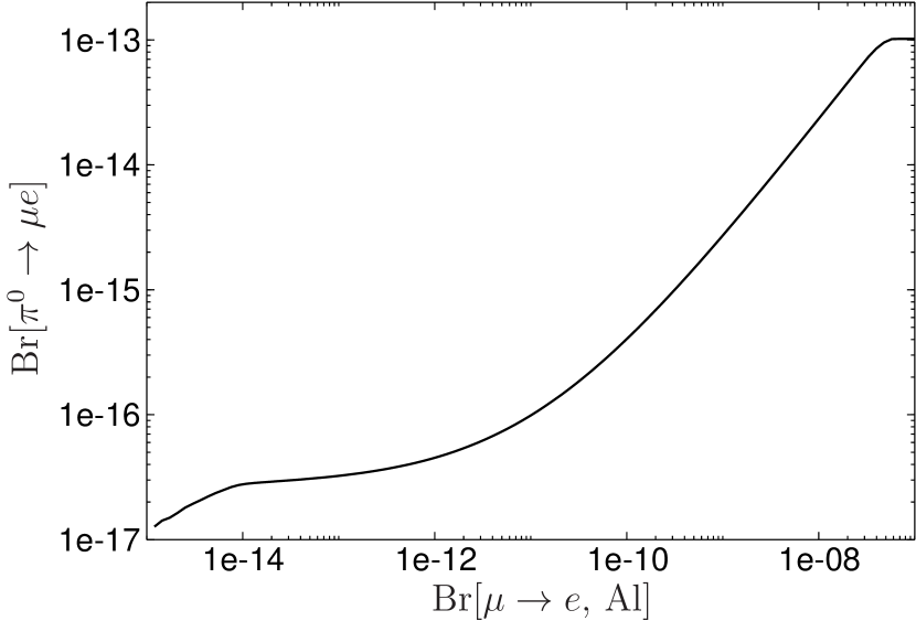
Figure 1: Limits on $\text{Br}[\pi^{0}\to\mu e]$ derived from $\text{Br}[\mu\to e,\text{Ti}]$ Wintz (1998) in combination with a future limit on $\text{Br}[\mu\to e,\text{Al}]$. Already a moderate precision for the latter suffices to substantially reduce cancellations that otherwise dilute the limit from Eq. (19) to Eq. (21).

Equation (II) shows that each multipole in the transverse and longitudinal responses is squared separately, which in ⁴⁷Ti ($L=1,3,5$) and ⁴⁹Ti ($L=1,3,5,7$) leads to a total of $2\times 3+2\times 4=14$ positive definite quantities. Accordingly, the only way to tune the rate to zero is to consider the couplings directly to protons and neutrons. Such a cancellation occurs at

$$C_{Y}^{A,u} =C_{Y}^{A,d}, C_{Y}^{A,s} =-\frac{2C_{Y}^{A,u}g^{u,0}_{A}}{g_{A}^{s,N}},$$

$$\frac{C_{Y}^{P,u}}{m_{u}} =\frac{C_{Y}^{P,d}}{m_{d}}, \frac{C_{Y}^{P,s}}{m_{s}} =\frac{4\pi}{\Lambda}C_{Y}^{G\tilde{G}}\frac{2g_{A}^{u,0}}{g_{A}^{u,0}-g_{A}^{s,N}}.$$ (20)

Since the conditions not involving strangeness remove any isovector contribution, this implies that for this choice of Wilson coefficients $\text{Br}[\pi^{0}\to\mu e]$ vanishes as well. In this case, the limit is thus protected against accidental cancellation, and a scan over the parameter space establishes

$$\text{Br}[\pi^{0}\to\mu e]<1.2\times 10^{-13}$$ (21)

as a rigorous limit. For $\eta$, $\eta^{\prime}$ a nonvanishing contribution remains, but such fine-tuned solutions are not viable due to RG corrections. As an example, we consider the dimension-$6$ contribution from $C_{Y}^{A,u}=C_{Y}^{A,d}$. If generated at a high scale $\Lambda$ above the electroweak scale $M_{W}$, already the one-loop QED corrections below $M_{W}$ produce a vector operator Crivellin et al. (2017); Cirigliano et al. (2017)

$$C_{Y}^{V,q}\simeq-3Q_{q}\frac{\alpha}{\pi}\log\frac{M_{W}}{m_{N}}C_{Y}^{A,q},$$ (22)

with quark charges $Q_{u}=2/3$, $Q_{d}=-1/3$, and thus a contribution to the SI rate (10). This indirect constraint gives

$$\text{Br}[\eta\to\mu e] <3.8\times 10^{-18},$$

$$\text{Br}[{\eta^{\prime}}\to\mu e] <9.1\times 10^{-20},$$ (23)

and thus excludes the solution via $C_{Y}^{A,q}$. Therefore, a fine tuning of Wilson coefficients can relax the limits (19), but, realistically, only by a few orders of magnitude. Moreover, the cancellations that arise from the interference of isoscalar and isovector contributions can be substantially reduced by considering other $\mu\to e$ targets. Figure 1 illustrates this for $\text{Br}[\pi^{0}\to\mu e]$ as a function of a future limit for $\mu\to e$ conversion in Al in combination with the current Ti constraint.

IV Conclusions

In this Letter, we studied the connection between LFV decays of the light pseudoscalars $P=\pi^{0},\eta,\eta^{\prime}$ and $\mu\to e$ conversion in nuclei. The EFT approach shows that up to dimension $7$ only a few operators—axial-vector, pseudoscalar, and gluonic ones—contribute to the pseudoscalar decays, which at the same time can mediate the $\mu\to e$ conversion process albeit only by coupling to the nuclear spin. We derived master formulae for both processes to quantify their interplay, including all required hadronic matrix elements and the nuclear responses for Ti. Despite the lack of coherent enhancement for the spin-dependent response, we found that, in general, the indirect limits for $P\to\mu e$ as derived from the current $\mu\to e$ conversion limit in Ti surpass the direct ones by many orders of magnitude. Fine-tuning Wilson coefficients can relax these limits to some extent, especially for $\eta$, $\eta^{\prime}$, but RG corrections curtail the amount of cancellations. The indirect limits presented here will further advance in the future with forthcoming measurements of $\mu\to e$ conversion in Al at the Mu2e and COMET experiments.

Appendix A Nuclear responses

Figure 2 assesses the quality of the nuclear shell-model calculation by comparing calculated low-lying spectra of ⁴⁷Ti, ⁴⁹Ti, and ²⁷Al with experiment ens . In all three cases the agreement is very good. For a comparison for ²⁷Al including higher excitation energies, see Ref. Klos et al. (2013). Also, Table 4 compares calculated charge radii with experimental values and presents the shell-model results for the spin expectation values $\langle\mathbf{S}_{N}\rangle$.

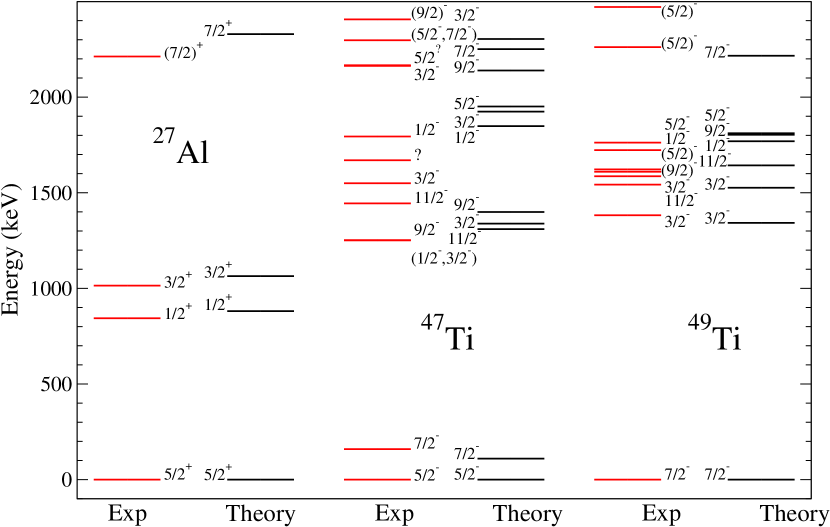
Figure 2: Calculated spectra of ²⁷Al, ⁴⁷Ti, and ⁴⁹Ti compared to experimental data ens . Only positive (negative) parity states are shown for ²⁷Al (^47,49Ti).

The nuclear shell-model interactions used in this work have also been used to study, in nuclei with similar mass as Al and Ti, other operators related to axial currents involving the nuclear spin such as Gamow–Teller $\beta$ decays. Calculations indicate that matrix elements are systematically overestimated, a deficiency related to the absence of two-body currents in the calculations Gysbers et al. (2019). Results obtained with other shell-model interactions different to the ones used in our work are in general very similar, typically within $10\%$ Richter et al. (2008); Kumar et al. (2016). In contrast, isoscalar magnetic dipole transitions, also spin-dependent, are well reproduced in the Al region Matsubara et al. (2015). In order to take into account these aspects, $\delta^{\prime}$ and $\delta^{\prime\prime}$ in Eq. (15) include the effect of two-body currents, with an uncertainty that their effect at $|\mathbf{q}|=0$, appropriate for Gamow–Teller decays, ranges from $20\%$–$30\%$. For the USDB interaction used for Al this effect is expected to be $23\%$ Richter et al. (2008) ($21\%$ for an alternative shell-model interaction in the same configuration space Richter et al. (2008)) and for KB3G $26\%$ Martínez-Pinedo et al. (1996) ($23\%$ for an alternative shell-model interaction Kumar et al. (2016)). Therefore, our uncertainty in $\delta^{\prime}$ and $\delta^{\prime\prime}$ covers also the expected nuclear uncertainty from using alternative nuclear shell-model interactions.

Table 5 summarizes the nuclear shell-model results for the $M$ and $\Phi^{\prime\prime}$ multipoles for all stable Ti and Al isotopes, while Tables 6 and 7 show the results for $\Sigma^{\prime}$, $\Sigma^{\prime\prime}$, following the conventions from Ref. Hoferichter et al. (2020). In all cases proton/neutron and isoscalar/isovector components are related by $\mathcal{F}_{\pm}(\mathbf{q}^{2})=\mathcal{F}_{p}(\mathbf{q}^{2})\pm\mathcal{F}_{n}(\mathbf{q}^{2})$. The SD structure factors are

$$S_{00}^{\mathcal{T}} =\sum_{L}\Big{[}\mathcal{F}_{+}^{\Sigma^{\prime}_{L}}(\mathbf{q}^{2})\Big{]}^{2}, S_{00}^{\mathcal{L}} =\sum_{L}\Big{[}\mathcal{F}_{+}^{\Sigma^{\prime\prime}_{L}}(\mathbf{q}^{2})\Big{]}^{2},$$

$$S_{11}^{\mathcal{T}} =\sum_{L}\Big{[}\mathcal{F}_{-}^{\Sigma^{\prime}_{L}}(\mathbf{q}^{2})\Big{]}^{2}, S_{11}^{\mathcal{L}} =\sum_{L}\Big{[}\mathcal{F}_{-}^{\Sigma^{\prime\prime}_{L}}(\mathbf{q}^{2})\Big{]}^{2},$$

$$S_{01}^{\mathcal{T}} =\sum_{L}2\mathcal{F}_{+}^{\Sigma^{\prime}_{L}}(\mathbf{q}^{2})\,\mathcal{F}_{-}^{\Sigma^{\prime}_{L}}(\mathbf{q}^{2}),$$

$$S_{01}^{\mathcal{L}} =\sum_{L}2\mathcal{F}_{+}^{\Sigma^{\prime\prime}_{L}}(\mathbf{q}^{2})\,\mathcal{F}_{-}^{\Sigma^{\prime\prime}_{L}}(\mathbf{q}^{2}),$$ (24)

with multipoles normalized as

$$\mathcal{F}_{N}^{\Sigma^{\prime}_{1}}(0)=\sqrt{2}\,\mathcal{F}_{N}^{\Sigma^{\prime\prime}_{1}}(0)=\sqrt{\frac{2}{3}}\sqrt{\frac{(2J+1)(J+1)}{4\pi J}}\langle\mathbf{S}_{N}\rangle.$$ (25)

	$R_{\text{ch}}^{\text{th}}$ [fm]	$R_{\text{ch}}^{\text{exp}}$ [fm]	$\langle\mathbf{S}_{p}\rangle$	$\langle\mathbf{S}_{n}\rangle$
46Ti	$3.59$	$3.6070(22)$	–	–
47Ti	$3.59$	$3.5962(19)$	$0.026$	$0.293$
48Ti	$3.60$	$3.5921(17)$	–	–
49Ti	$3.61$	$3.5733(21)$	$0.028$	$0.367$
50Ti	$3.62$	$3.5704(22)$	–	–
27Al	$3.14$	$3.0610(31)$	$0.326$	$0.038$

Table 4: Theoretical charge radii compared to experiment from Ref. Angeli and Marinova (2013), as well as calculated proton ($\langle\mathbf{S}_{p}\rangle$) and neutron ($\langle\mathbf{S}_{n}\rangle$) spin expectation values.

Isotope	46Ti	47Ti	48Ti	49Ti	50Ti	27Al
$J^{P}$	$0^{+}$	$5/2^{-}$	$0^{+}$	$7/2^{-}$	$0^{+}$	$5/2^{+}$
$\eta$ [%]	$8.25(3)$	$7.44(2)$	$73.72(3)$	$5.41(2)$	$5.18(2)$	$100$
$b$ [fm]	$1.9769$	$1.9827$	$1.9884$	$1.9940$	$1.9995$	$1.8420$
$c_{1}^{M+}$	$-25.9987$	$-27.0005$	$-28.0021$	$-28.9986$	$-29.9991$	$-11.3343$
$c_{2}^{M+}$	$3.28239$	$3.49161$	$3.6798$	$3.85975$	$4.05453$	$0.837814$
$c_{3}^{M+}$	$-0.0685135$	$-0.0797877$	$-0.088061$	$-0.0939764$	$-0.102896$	–
$c_{1}^{M-}$	$1.99997$	$2.99993$	$4.00016$	$4.99982$	$5.99979$	$0.666696$
$c_{2}^{M-}$	$-0.406935$	$-0.617487$	$-0.830249$	$-1.03009$	$-1.2358$	$-0.0858552$
$c_{3}^{M-}$	$0.0200208$	$0.0310325$	$0.0424272$	$0.0518767$	$0.062231$	–
$c_{0}^{\Phi^{\prime\prime}+}$	$-4.73881$	$-5.91242$	$-6.77176$	$-7.96954$	$-8.91559$	$-4.98975$
$c_{1}^{\Phi^{\prime\prime}+}$	$1.8957$	$2.365$	$2.70879$	$3.18778$	$3.566129$	$0.997985$
$c_{2}^{\Phi^{\prime\prime}+}$	$-0.140202$	$-0.175856$	$-0.198666$	$-0.231598$	$-0.25760$	–
$c_{0}^{\Phi^{\prime\prime}-}$	$1.61434$	$2.67922$	$3.45274$	$4.5949$	$5.54649$	$0.303398$
$c_{1}^{\Phi^{\prime\prime}-}$	$-0.645785$	$-1.07173$	$-1.38116$	$-1.8379$	$-2.2185$	$-0.0606814$
$c_{2}^{\Phi^{\prime\prime}-}$	$0.0461341$	$0.0771383$	$0.100134$	$0.133188$	$0.160647$	–

Table 5: Spin/parity $J^{P}$ of the nuclear ground states, natural abundance $\eta$, harmonic-oscillator length $b$, and fit coefficients for the nuclear multipoles $\mathcal{F}_{\pm}^{M}$ and $\mathcal{F}_{\pm}^{\Phi^{\prime\prime}}$. The parameterizations $\mathcal{F}_{\pm}^{M}(u)=e^{-\frac{u}{2}}\sum_{i=0}^{3}c_{i}^{M\pm}u^{i}$ (with $c_{0}^{M+}=Z+N$ and $c_{0}^{M-}=Z-N$) and $\mathcal{F}_{\pm}^{\Phi^{\prime\prime}}(u)=e^{-\frac{u}{2}}\sum_{i=0}^{2}c_{i}^{\Phi^{\prime\prime}\pm}u^{i}$, with $u=\mathbf{q}^{2}b^{2}/2$, correspond to the analytical form in the harmonic-oscillator basis Donnelly and Haxton (1979).

Isotope	47Ti			49Ti
$L$	$1$	$3$	$5$	$1$	$3$	$5$	$7$
$c_{0}^{\Sigma^{\prime}p}$	$0.0175579$	–	–	$0.0203333$	–	–	–
$c_{1}^{\Sigma^{\prime}p}$	$-0.0179636$	$0.00453093$	–	$-0.0214563$	$-0.00759501$	–	–
$c_{2}^{\Sigma^{\prime}p}$	$0.00314365$	$-0.00134858$	$-0.0000163753$	$0.00397767$	$0.00354166$	$-0.00043197$	–
$c_{3}^{\Sigma^{\prime}p}$	$-0.0000982683$	$0.0000307488$	$0.0000216414$	$-0.000155929$	$-0.000272126$	$0.0000408714$	$-2.75178\times 10^{-6}$
$c_{0}^{\Sigma^{\prime}n}$	$0.19529$	–	–	$0.271019$	–	–	–
$c_{1}^{\Sigma^{\prime}n}$	$-0.245141$	$0.0279757$	–	$-0.357078$	$-0.129809$	–	–
$c_{2}^{\Sigma^{\prime}n}$	$0.0551808$	$-0.0120502$	$-0.0298524$	$0.0813202$	$0.0399765$	$0.0179357$	–
$c_{3}^{\Sigma^{\prime}n}$	$-0.00288588$	$0.0010701$	$0.00255996$	$-0.00432571$	$-0.00229466$	$-0.00108624$	$-0.00576536$
$c_{0}^{\Sigma^{\prime\prime}p}$	$0.0124152$	–	–	$0.0143777$	–	–	–
$c_{1}^{\Sigma^{\prime\prime}p}$	$-0.0118426$	$0.00392391$	–	$-0.0127874$	$-0.00657747$	–	–
$c_{2}^{\Sigma^{\prime\prime}p}$	$0.00272966$	$-0.000701449$	$-0.0000149486$	$0.00252953$	$0.00196317$	$-0.000394335$	–
$c_{3}^{\Sigma^{\prime\prime}p}$	$-0.000176902$	$0.0000103558$	$0.0000122962$	$-0.000122398$	$-0.000120552$	$0.0000438309$	$-2.57402\times 10^{-6}$
$c_{0}^{\Sigma^{\prime\prime}n}$	$0.138089$	–	–	$0.191638$	–	–	–
$c_{1}^{\Sigma^{\prime\prime}n}$	$-0.0676043$	$0.0242274$	–	$-0.0699121$	$-0.112418$	–	–
$c_{2}^{\Sigma^{\prime\prime}n}$	$0.00783041$	$-0.00458878$	$-0.0272513$	$0.00435709$	$0.0179024$	$0.0163729$	–
$c_{3}^{\Sigma^{\prime\prime}n}$	$-0.000298162$	$0.000464503$	$0.00168688$	$0.0000212473$	$-0.000600979$	$-0.000188205$	$-0.00539299$

Table 6: Fit coefficients for the nuclear multipoles $\mathcal{F}_{N}^{\Sigma^{\prime}_{L}}$ and $\mathcal{F}_{N}^{\Sigma^{\prime\prime}_{L}}$ of ^47,49Ti, using the fit function $\mathcal{F}(u)=e^{-\frac{u}{2}}\sum_{i=0}^{3}c_{i}u^{i}$.

Isotope	27Al
$L$	$1$	$3$	$5$
$c_{0}^{\Sigma^{\prime}p}$	$0.217688$	–	–
$c_{1}^{\Sigma^{\prime}p}$	$-0.199127$	$-0.0543796$	–
$c_{2}^{\Sigma^{\prime}p}$	$0.0274599$	$0.00651646$	$0.0277341$
$c_{0}^{\Sigma^{\prime}n}$	$0.0255784$	–	–
$c_{1}^{\Sigma^{\prime}n}$	$-0.00985665$	$0.000280434$	–
$c_{2}^{\Sigma^{\prime}n}$	$-0.00150251$	$-0.000488419$	$0.000128524$
$c_{0}^{\Sigma^{\prime\prime}p}$	$0.153928$	–	–
$c_{1}^{\Sigma^{\prime\prime}p}$	$-0.0262479$	$-0.0470943$	–
$c_{2}^{\Sigma^{\prime\prime}p}$	$0.00103769$	$-0.00206298$	$0.0253177$
$c_{0}^{\Sigma^{\prime\prime}n}$	$0.0180868$	–	–
$c_{1}^{\Sigma^{\prime\prime}n}$	$-0.022234$	$0.000242867$	–
$c_{2}^{\Sigma^{\prime\prime}n}$	$0.00278141$	$0.000103865$	$0.000117327$

Table 7: Same as Table 6 for ²⁷Al.

Appendix B Matrix elements of $\boldsymbol{G\tilde{G}}$

At present, no model-independent determination of the nucleon matrix element of the $G^{a}_{\mu\nu}\tilde{G}_{a}^{\mu\nu}$ operator is available, and an additional condition is necessary to solve for all couplings $g_{5}^{q,N}$, $\tilde{a}_{N}$ in Eq. (17). As suggested by large-$N_{c}$ arguments, frequently one imposes Cheng and Chiang (2012)

$$\langle N|\sum_{q}\bar{q}i\gamma_{5}q|N\rangle=0.$$ (26)

As a first step, we study the consequences of the analog condition for the case of the pseudoscalar matrix elements. Imposing $\sum_{q}b_{q}h_{P}^{q}/m_{q}=0$, we solve Eq. (7) to obtain

$$a_{P}^{\text{FKS}}=-\frac{M_{P}^{2}(b_{u}f_{P}^{u}+b_{d}f_{P}^{d})}{2},$$ (27)

where we expanded in $m_{u,d}\ll m_{s}$ and assumed the isospin limit, as throughout this work. The approximation (27) coincides with the result in the FKS $\eta$–$\eta^{\prime}$ mixing scheme: starting from Beneke and Neubert (2003)

$$a_{\eta}^{\text{FKS}} =-\frac{M_{\eta^{\prime}}^{2}-M_{\eta}^{2}}{2\sqrt{2}}\sin(2\phi)\Big{[}-f_{q}\sin\phi+\sqrt{2}f_{s}\cos\phi\Big{]},$$

$$a_{\eta^{\prime}}^{\text{FKS}} =-\frac{M_{\eta^{\prime}}^{2}-M_{\eta}^{2}}{2\sqrt{2}}\sin(2\phi)\Big{[}f_{q}\cos\phi+\sqrt{2}f_{s}\sin\phi\Big{]},$$ (28)

with

$$f_{\eta}^{u} =f_{\eta}^{d}=f_{q}\cos\phi, f_{\eta}^{s} =-f_{s}\sin\phi,$$

$$f_{\eta^{\prime}}^{u} =f_{\eta^{\prime}}^{d}=f_{q}\sin\phi, f_{\eta^{\prime}}^{s} =f_{s}\cos\phi,$$ (29)

expressed in terms of a single mixing angle $\phi$, the expression (27) is indeed reproduced upon using Feldmann et al. (1998)

$$\frac{\sqrt{2}f_{s}}{f_{q}}=\tan(\phi-\theta_{8}),\qquad\cot\theta_{8}=-\frac{M_{\eta^{\prime}}^{2}}{M_{\eta}^{2}}\tan\phi,$$ (30)

with the latter also assuming the $m_{u,d}\ll m_{s}$ limit. Table 1 indicates that the results obtained in this way agree well with the lattice calculation of Ref. Bali et al. (2021). Since the corrections to the FKS scheme are indeed expected to be suppressed in the large-$N_{c}$ limit, it appears natural that the large-$N_{c}$ arguments from Ref. Cheng and Chiang (2012) lead to the same result. In addition, the numerical agreement for the pseudoscalar matrix elements suggests that the corresponding estimate for the nucleon case (18) is reasonable as well. Note that, in contrast to Ref. Cheng and Chiang (2012), we evaluate this estimate again in the isospin limit, since corrections can only be assessed in a consistent manner considering also isospin-breaking effects in the axial-vector couplings $g_{A}^{q,N}$.

References

- Petcov (1977) S. T. Petcov, Sov. J. Nucl. Phys. 25, 340 (1977), [Yad. Fiz. 25, 641 (1977), Erratum: Sov. J. Nucl. Phys. 25, 698 (1977), Yad. Fiz. 25, 1336 (1977)].
- Marciano and Sanda (1977a) W. J. Marciano and A. I. Sanda, Phys. Lett. B 67, 303 (1977a).
- Marciano and Sanda (1977b) W. J. Marciano and A. I. Sanda, Phys. Rev. Lett. 38, 1512 (1977b).
- Lee et al. (1977) B. W. Lee, S. Pakvasa, R. E. Shrock, and H. Sugawara, Phys. Rev. Lett. 38, 937 (1977), [Erratum: Phys. Rev. Lett. 38, 1230 (1977)].
- Lee and Shrock (1977) B. W. Lee and R. E. Shrock, Phys. Rev. D 16, 1444 (1977).
- Kuno and Okada (2001) Y. Kuno and Y. Okada, Rev. Mod. Phys. 73, 151 (2001), eprint hep-ph/9909265.
- Mihara et al. (2013) S. Mihara, J. P. Miller, P. Paradisi, and G. Piredda, Ann. Rev. Nucl. Part. Sci. 63, 531 (2013).
- Calibbi and Signorelli (2018) L. Calibbi and G. Signorelli, Riv. Nuovo Cim. 41, 71 (2018), eprint 1709.00294.
- Baldini et al. (2016) A. M. Baldini et al. (MEG), Eur. Phys. J. C 76, 434 (2016), eprint 1605.05081.
- Bellgardt et al. (1988) U. Bellgardt et al. (SINDRUM), Nucl. Phys. B 299, 1 (1988).
- Wintz (1998) P. Wintz, Conf. Proc. C 980420, 534 (1998).
- Bertl et al. (2006) W. H. Bertl et al. (SINDRUM II), Eur. Phys. J. C 47, 337 (2006).
- Suzuki et al. (1987) T. Suzuki, D. F. Measday, and J. P. Roalsvig, Phys. Rev. C 35, 2212 (1987).
- Dohmen et al. (1993) C. Dohmen et al. (SINDRUM II), Phys. Lett. B 317, 631 (1993).
- Baldini et al. (2018) A. M. Baldini et al. (MEG II), Eur. Phys. J. C 78, 380 (2018), eprint 1801.04688.
- Arndt et al. (2021) K. Arndt et al. (Mu3e), Nucl. Instrum. Meth. A 1014, 165679 (2021), eprint 2009.11690.
- Aiba et al. (2021) M. Aiba et al. (2021), eprint 2111.05788.
- Bartoszek et al. (2014) L. Bartoszek et al. (Mu2e) (2014), eprint 1501.05241.
- Abramishvili et al. (2020) R. Abramishvili et al. (COMET), PTEP 2020, 033C01 (2020), eprint 1812.09018.
- Zyla et al. (2020) P. A. Zyla et al. (Particle Data Group), PTEP 2020, 083C01 (2020).
- Appel et al. (2000a) R. Appel et al., Phys. Rev. Lett. 85, 2450 (2000a), eprint hep-ex/0005016.
- Cortina Gil et al. (2021) E. Cortina Gil et al. (NA62), Phys. Rev. Lett. 127, 131802 (2021), eprint 2105.06759.
- Abouzaid et al. (2008) E. Abouzaid et al. (KTeV), Phys. Rev. Lett. 100, 131803 (2008), eprint 0711.3472.
- White et al. (1996) D. B. White et al., Phys. Rev. D 53, 6658 (1996).
- Briere et al. (2000) R. A. Briere et al. (CLEO), Phys. Rev. Lett. 84, 26 (2000), eprint hep-ex/9907046.
- Appel et al. (2000b) R. Appel et al., Phys. Rev. Lett. 85, 2877 (2000b), eprint hep-ex/0006003.
- (27) L. Gan et al., Eta Decays with Emphasis on Rare Neutral Modes: The JLab Eta Factory (JEF) Experiment, JLab proposal, https://www.jlab.org/exp_prog/proposals/14/PR12-14-004.pdf.
- Elam et al. (2022) J. Elam et al. (REDTOP) (2022), eprint 2203.07651.
- Petrov and Zhuridov (2014) A. A. Petrov and D. V. Zhuridov, Phys. Rev. D 89, 033005 (2014), eprint 1308.6561.
- Crivellin et al. (2014a) A. Crivellin, S. Najjari, and J. Rosiek, JHEP 04, 167 (2014a), eprint 1312.0634.
- Hazard and Petrov (2016) D. E. Hazard and A. A. Petrov, Phys. Rev. D 94, 074023 (2016), eprint 1607.00815.
- Crivellin et al. (2017) A. Crivellin, S. Davidson, G. M. Pruna, and A. Signer, JHEP 05, 117 (2017), eprint 1702.03020.
- Cirigliano et al. (2017) V. Cirigliano, S. Davidson, and Y. Kuno, Phys. Lett. B 771, 242 (2017), eprint 1703.02057.
- Davidson et al. (2019) S. Davidson, Y. Kuno, and M. Yamanaka, Phys. Lett. B 790, 380 (2019), eprint 1810.01884.
- Davidson (2021) S. Davidson, JHEP 02, 172 (2021), eprint 2010.00317.
- Davidson and Echenard (2022) S. Davidson and B. Echenard, Eur. Phys. J. C 82, 836 (2022), eprint 2204.00564.
- Davidson et al. (2018) S. Davidson, Y. Kuno, and A. Saporta, Eur. Phys. J. C 78, 109 (2018), eprint 1710.06787.
- Gan et al. (2022) L. Gan, B. Kubis, E. Passemar, and S. Tulin, Phys. Rept. 945, 2191 (2022), eprint 2007.00664.
- Beneke and Neubert (2003) M. Beneke and M. Neubert, Nucl. Phys. B 651, 225 (2003), eprint hep-ph/0210085.
- Escribano et al. (2016) R. Escribano, S. Gonzàlez-Solís, P. Masjuan, and P. Sánchez-Puertas, Phys. Rev. D 94, 054033 (2016), eprint 1512.07520.
- Bali et al. (2021) G. S. Bali, V. Braun, S. Collins, A. Schäfer, and J. Simeth (RQCD), JHEP 08, 137 (2021), eprint 2106.05398.
- Feldmann et al. (1998) T. Feldmann, P. Kroll, and B. Stech, Phys. Rev. D 58, 114006 (1998), eprint hep-ph/9802409.
- (43) F. Noël et al., in preparation.
- Serot (1978) B. D. Serot, Nucl. Phys. A 308, 457 (1978).
- Donnelly and Peccei (1979) T. W. Donnelly and R. D. Peccei, Phys. Rept. 50, 1 (1979).
- Donnelly and Haxton (1979) T. W. Donnelly and W. C. Haxton, Atom. Data Nucl. Data Tabl. 23, 103 (1979).
- Walecka (1995) J. D. Walecka, Theoretical nuclear and subnuclear physics, vol. 16 (1995).
- Glick-Magid and Gazit (2022) A. Glick-Magid and D. Gazit (2022), eprint 2207.01357.
- Klos et al. (2013) P. Klos, J. Menéndez, D. Gazit, and A. Schwenk, Phys. Rev. D 88, 083516 (2013), [Erratum: Phys. Rev. D 89, 029901 (2014)], eprint 1304.7684.
- Hoferichter et al. (2015a) M. Hoferichter, P. Klos, and A. Schwenk, Phys. Lett. B 746, 410 (2015a), eprint 1503.04811.
- Hoferichter et al. (2016a) M. Hoferichter, P. Klos, J. Menéndez, and A. Schwenk, Phys. Rev. D 94, 063505 (2016a), eprint 1605.08043.
- Hoferichter et al. (2017) M. Hoferichter, P. Klos, J. Menéndez, and A. Schwenk, Phys. Rev. Lett. 119, 181803 (2017), eprint 1708.02245.
- Aprile et al. (2019) E. Aprile et al. (XENON), Phys. Rev. Lett. 122, 071301 (2019), eprint 1811.12482.
- Hoferichter et al. (2019a) M. Hoferichter, P. Klos, J. Menéndez, and A. Schwenk, Phys. Rev. D 99, 055031 (2019a), eprint 1812.05617.
- Hoferichter et al. (2020) M. Hoferichter, J. Menéndez, and A. Schwenk, Phys. Rev. D 102, 074018 (2020), eprint 2007.08529.
- Kitano et al. (2002) R. Kitano, M. Koike, and Y. Okada, Phys. Rev. D 66, 096002 (2002), [Erratum: Phys. Rev. D 76, 059902 (2007)], eprint hep-ph/0203110.
- De Vries et al. (1987) H. De Vries, C. W. De Jager, and C. De Vries, Atom. Data Nucl. Data Tabl. 36, 495 (1987).
- Cirigliano et al. (2009) V. Cirigliano, R. Kitano, Y. Okada, and P. Tuzon, Phys. Rev. D 80, 013002 (2009), eprint 0904.0957.
- Crivellin et al. (2014b) A. Crivellin, M. Hoferichter, and M. Procura, Phys. Rev. D 89, 054021 (2014b), eprint 1312.4951.
- Crivellin et al. (2014c) A. Crivellin, M. Hoferichter, and M. Procura, Phys. Rev. D 89, 093024 (2014c), eprint 1404.7134.
- Hoferichter et al. (2015b) M. Hoferichter, J. Ruiz de Elvira, B. Kubis, and U.-G. Meißner, Phys. Rev. Lett. 115, 092301 (2015b), eprint 1506.04142.
- Ruiz de Elvira et al. (2018) J. Ruiz de Elvira, M. Hoferichter, B. Kubis, and U.-G. Meißner, J. Phys. G 45, 024001 (2018), eprint 1706.01465.
- Gupta et al. (2021) R. Gupta, S. Park, M. Hoferichter, E. Mereghetti, B. Yoon, and T. Bhattacharya, Phys. Rev. Lett. 127, 242002 (2021), eprint 2105.12095.
- Shifman et al. (1978) M. A. Shifman, A. I. Vainshtein, and V. I. Zakharov, Phys. Lett. B 78, 443 (1978).
- Cirigliano et al. (2022) V. Cirigliano, K. Fuyuto, M. J. Ramsey-Musolf, and E. Rule, Phys. Rev. C 105, 055504 (2022), eprint 2203.09547.
- Hoferichter et al. (2012) M. Hoferichter, C. Ditsche, B. Kubis, and U.-G. Meißner, JHEP 06, 063 (2012), eprint 1204.6251.
- Rule et al. (2021) E. Rule, W. C. Haxton, and K. McElvain (2021), eprint 2109.13503.
- Caurier et al. (2005) E. Caurier, G. Martínez-Pinedo, F. Nowacki, A. Poves, and A. P. Zuker, Rev. Mod. Phys. 77, 427 (2005), eprint nucl-th/0402046.
- Otsuka et al. (2020) T. Otsuka, A. Gade, O. Sorlin, T. Suzuki, and Y. Utsuno, Rev. Mod. Phys. 92, 015002 (2020), eprint 1805.06501.
- Caurier and Nowacki (1999) E. Caurier and F. Nowacki, Acta Phys. Pol. 30, 705 (1999).
- Poves et al. (2001) A. Poves, J. Sánchez-Solano, E. Caurier, and F. Nowacki, Nucl. Phys. A 694, 157 (2001), eprint nucl-th/0012077.
- Brown and Richter (2006) B. A. Brown and W. A. Richter, Phys. Rev. C 74, 034315 (2006).
- (73) The appendix provides details of the nuclear shell-model calculations (including Refs. ens ; Richter et al. (2008); Kumar et al. (2016); Matsubara et al. (2015); Martínez-Pinedo et al. (1996); Angeli and Marinova (2013)) and the matrix elements.
- (74) https://www.nndc.bnl.gov/ensdf/.
- Richter et al. (2008) W. A. Richter, S. Mkhize, and B. A. Brown, Phys. Rev. C 78, 064302 (2008).
- Kumar et al. (2016) V. Kumar, P. C. Srivastava, and J. G. Hirsch, Eur. Phys. J. A 52, 181 (2016), eprint 1511.03887.
- Matsubara et al. (2015) H. Matsubara et al., Phys. Rev. Lett. 115, 102501 (2015).
- Martínez-Pinedo et al. (1996) G. Martínez-Pinedo, A. Poves, E. Caurier, and A. P. Zuker, Phys. Rev. C 53, R2602 (1996), eprint nucl-th/9603039.
- Angeli and Marinova (2013) I. Angeli and K. P. Marinova, Atom. Data Nucl. Data Tabl. 99, 69 (2013).
- Gysbers et al. (2019) P. Gysbers et al., Nature Phys. 15, 428 (2019), eprint 1903.00047.
- Hoferichter et al. (2015c) M. Hoferichter, J. Ruiz de Elvira, B. Kubis, and U.-G. Meißner, Phys. Rev. Lett. 115, 192301 (2015c), eprint 1507.07552.
- Hoferichter et al. (2016b) M. Hoferichter, J. Ruiz de Elvira, B. Kubis, and U.-G. Meißner, Phys. Rept. 625, 1 (2016b), eprint 1510.06039.
- Airapetian et al. (2007) A. Airapetian et al. (HERMES), Phys. Rev. D 75, 012007 (2007), eprint hep-ex/0609039.
- Liang et al. (2018) J. Liang, Y.-B. Yang, T. Draper, M. Gong, and K.-F. Liu, Phys. Rev. D 98, 074505 (2018), eprint 1806.08366.
- Lin et al. (2018) H.-W. Lin, R. Gupta, B. Yoon, Y.-C. Jang, and T. Bhattacharya, Phys. Rev. D 98, 094512 (2018), eprint 1806.10604.
- Aoki et al. (2022) Y. Aoki et al. (Flavour Lattice Averaging Group (FLAG)), Eur. Phys. J. C 82, 869 (2022), eprint 2111.09849.
- Cheng (1989) H.-Y. Cheng, Phys. Lett. B 219, 347 (1989).
- Cheng and Chiang (2012) H.-Y. Cheng and C.-W. Chiang, JHEP 07, 009 (2012), eprint 1202.1292.
- Dragos et al. (2021) J. Dragos, T. Luu, A. Shindler, J. de Vries, and A. Yousif, Phys. Rev. C 103, 015202 (2021), eprint 1902.03254.
- Bhattacharya et al. (2021) T. Bhattacharya, V. Cirigliano, R. Gupta, E. Mereghetti, and B. Yoon, Phys. Rev. D 103, 114507 (2021), eprint 2101.07230.
- Gupta et al. (2018) R. Gupta, B. Yoon, T. Bhattacharya, V. Cirigliano, Y.-C. Jang, and H.-W. Lin, Phys. Rev. D 98, 091501 (2018), eprint 1808.07597.
- Hoferichter et al. (2019b) M. Hoferichter, B. Kubis, J. Ruiz de Elvira, and P. Stoffer, Phys. Rev. Lett. 122, 122001 (2019b), [Erratum: Phys. Rev. Lett. 124, 199901 (2020)], eprint 1811.11181.