Probing carrier interactions using electron hydrodynamics

Abstract

Electron hydrodynamics arises when momentum-relaxing scattering processes are slow compared to momentum-conserving ones. While the microscopic details necessary to satisfy this condition are material-specific, experimentally accessible current densities share remarkable similarities. We study the dependence of electron hydrodynamic flows on the rates of momentum-relaxing and momentum-conserving scattering processes in a microscopics-agnostic way. We develop a framework for generating random collision operators which respect crystal symmetries and conservation laws and which have a tunable ratio between the momentum-conserving and momentum-relaxing lifetimes. Using various random instances of these collision operators, we calculate macroscopic electron viscosity tensors and solve the Boltzmann transport equation (BTE) in a channel geometry over a grid of momentum-conserving and momentum-relaxing lifetimes, and for different crystal symmetry groups. We find that different random collision operators using the same lifetimes produce very similar current density profiles, meaning that the current density is primarily a probe of the overall rates of momentum conservation and relaxation. By contrast, the viscosity tensor varies substantially at fixed lifetimes, meaning that properties like channel resistance provide detailed probes of the underlying scattering processes. This suggests that, while details of the scattering process are imprinted in the electronic viscosity tensor, for many applications theoretical calculations of hydrodynamic electron flows can use experimentally-available lifetimes within a spatially-resolved BTE framework rather than requiring the costly computation of ab initio collision operators.

I Introduction

Spatially-resolved experiments have revealed that electrons in condensed matter can flow collectively akin to classical fluids Krishna Kumar et al. (2017); Sulpizio et al. (2019); Marguerite et al. (2019); Ku et al. (2020); Jenkins et al. (2020), confirming theoretical predictions over fifty years old Gurzhi (1968). Such electron “hydrodynamics” is observed in the limit where microscopic momentum-relaxing interactions, for example, scattering of electrons against impurities and/or lattice vibrations, are slow compared to momentum-conserving electron-electron interactions, such as the repulsive Coulomb interaction.

Since electron screening effects are expected to minimize direct (Coulomb) electron-electron interactions in bulk conductors, the seemingly-serendipitous observations of electron hydrodynamics in bulk (semi-)metals Moll et al. (2016); Gooth et al. (2018); Osterhoudt et al. (2021); Vool et al. (2021); Aharon-Steinberg et al. (2022) have garnered significant attention, and recent work attributes these to indirect lattice-mediated electron interactions Vool et al. (2021); Varnavides et al. (2022); Wang et al. (2021). Despite the differences in the microscopic origins of momentum-conserving interactions, the hallmark features of channel or “Poiseuille” flow, that is, enhanced current density in the center of the channel and reduced current density at the edges Sulpizio et al. (2019); Ku et al. (2020); Jenkins et al. (2020); Vool et al. (2021), appear similar.

At the same time, the theoretical methods used to investigate these electron hydrodynamic flows often rely on simplifying models, such as the electronic Stokes equations Mendoza et al. (2011); Levitov and Falkovich (2016); Guo et al. (2017); Varnavides et al. (2020); Scaffidi et al. (2017); Kiselev and Schmalian (2019) and the dual relaxation time approximation of the Boltzmann transport equation Govorov and Heremans (2004); Cepellotti et al. (2015); Guo et al. (2016); Scaffidi et al. (2017); Ledwith et al. (2019); Kiselev and Schmalian (2019); Callaway (1959); Guyer and Krumhansl (1966); de Jong and Molenkamp (1995). The former is only strictly valid in the unphysical limit of zero momentum relaxation, while the latter effectively convolves all microscopic details to arrive at scalar lifetimes which greatly simplify the kinetic theory used.

More recently, numerical methods to solve the linearized Boltzmann transport equation iteratively with spatial-resolution have been developed and applied to study plasmonic hot carriers Jermyn et al. (2019), and phonon transport Varnavides et al. (2019); Romano (2020). While these methods allow one to go beyond the dual relaxation time approximation, it is computationally expensive to calculate the linearized collision operator for electron interactions from first principles.

Taken together, these observations pose questions that are key to our understanding of electron hydrodynamics:

1. How sensitive are macroscopic observables of electron hydrodynamic flows to microscopic interaction details?

2. Can we identify the linearized collision operator using experimentally-accessible scalar interaction lifetimes?

In this Article, we investigate these questions statistically. In section II we propose a procedure to construct physically-plausible random linearized collision operators using the crystal symmetry of the system in question and conservation laws of properties such as eigen-energies, group velocities, and scalar interaction lifetimes. The latter can be obtained using temperature-dependent first principle calculations Coulter et al. (2018); Garcia et al. (2021); Varnavides et al. (2022); Wang et al. (2021), or extracted from transport measurements Gooth et al. (2018); Vool et al. (2021). In section III we use the inherent randomness in the proposed procedure as a proxy for the differences introduced by the mechanism- and material-specific microscopic interaction details, and evaluate their variability on macroscopic observables, such as current density measurements in two-dimensional channel flow.

Two key findings emerge from our analysis: First, different random instances of the collision operator with the same interaction lifetimes produce very similar current density profiles. That is, the details of the scattering processes at work in a material do not set the current density; rather it is controlled by the overall rates of momentum conservation and relaxation. As a result experimental measurements of the current density profile probe these overall rates, not the details of the scattering processes at work. Secondly, the electron fluid’s viscosity tensor is sensitive to microscopic details of the collision operator. Its components vary by more than $\sim$50% between different collision operators. Thus the action of viscosity on the channel flow resistance provide an experimental probe of the underlying scattering processes. These observations are consistent across different crystal symmetry groups, and provide quantitative estimates of the error introduced by the dual relaxation time approximation.

Finally, we note that for most applications, the error introduced by approximating the linearized collision operator with experimentally-available lifetimes is within the experimental uncertainty of current profile measurements Sulpizio et al. (2019); Ku et al. (2020); Jenkins et al. (2020); Vool et al. (2021); Aharon-Steinberg et al. (2022), and provides a promising efficient alternative to ab-initio calculations.

II Formalism

II.1 Boltzmann Transport Equation

We consider the general transport problem given by the semi-classical Boltzmann transport equation (BTE):

$$\partial_{t}n_{i}(\bm{r})+\bm{v}_{i}\cdot\nabla_{\bm{r}}n_{i}(\bm{r})=-\bm{F}\cdot\nabla_{\bm{k}}n_{i}(\bm{r})-\Gamma_{i}[\{n_{j}(\bm{r})\}],$$ (1)

where $n_{i}(\bm{r})$ is the distribution function of carriers in combined state index $i$ (encompassing the wavevector $\bm{k}$ and band $\nu$), $\bm{v}_{i}$ is the group velocity of state $i$, $\bm{F}$ is an external driving force, and $\Gamma_{i}[\{n_{j}(\bm{r})\}]$ is the collision operator, which specifies the rate at which carriers scatter into and out of state $i$ as a function of the full carrier distribution $n_{j}(\bm{r})$ at position $\bm{r}$. A key observation underpinning our approach is that the collision operator is local in space, while the advection operator $\bm{v}_{i}\cdot\nabla_{\bm{r}}$ is local in state-space.

Our framework rests on several assumptions. First, we take the carrier distribution to be in steady state, eliminating the first term in equation (1). Next, we linearize the collision operator about an equilibrium distribution $n^{0}_{j}$, with

$$\delta n_{j}\equiv n_{j}-n^{0}_{j}$$ (2)

such that

$$\Gamma_{i}[\{n_{j}(\bm{r})\}]\approx\frac{\partial\Gamma_{i}}{\partial n_{j}}\delta n_{j},$$ (3)

where summation is implied over repeated indices. For fermions we take $n_{j}^{0}$ as the Fermi-Dirac distribution, while for bosons we take it as the Bose-Einstein distribution. Finally, we assume that the temperature and material properties are spatially uniform, such that $n^{0}_{j}$ is not a function of position and

$$-\bm{F}\cdot\nabla_{\bm{i}}n_{i}(\bm{r})\approx-\bm{v}_{i}\cdot\frac{\partial n_{i}^{0}}{\partial\epsilon_{i}}\bm{F}=S_{i},$$ (4)

where $\epsilon_{i}$ is the eigen-energy of state $i$, and we have identified the linearized forcing terms, which depend only on the equilibirum distribution, with a ‘source’ term $S_{i}$ of carriers in state $i$. With these assumptions, the BTE simplifies to

$$\bm{v}_{i}\cdot\nabla_{\bm{r}}\delta n_{i}(\bm{r})=S_{i}-\frac{\partial\Gamma_{i}}{\partial n_{j}}\delta n_{j}(\bm{r}).$$ (5)

Equation 5 can be re-written in the form:

$$\left(\frac{\partial\Gamma_{i}}{\partial n_{j}}+\delta_{ij}\bm{v}_{i}\cdot\nabla_{\bm{r}}\right)\delta n_{j}(\bm{r})=S_{i},$$ (6)

which highlights that the solution $\delta n_{j}(\bm{r})$ may be obtained by inverting the operator in parentheses. However, the operator to be inverted exists over the large joint space of spatial and state dimensions, so we proceed iteratively Jermyn et al. (2019); Varnavides et al. (2019). First, we separate the collision operator into diagonal terms, representing decay with lifetime $\tau_{i}$, and off-diagonal ‘mixing’ terms:

$$\frac{\partial\Gamma_{i}}{\partial n_{j}}=\tau_{i}^{-1}\delta_{ij}-M_{ij}.$$ (7)

Using this decomposition the BTE may be written as:

$$(1+\tau_{i}\bm{v}_{i}\cdot\nabla_{\bm{r}})\delta n_{i}(\bm{r})=\tau_{i}S_{i}+\tau_{i}M_{ij}\delta n_{j},$$ (8)

where the left-hand and right-hand sides contain only terms local in state- and position-space respectively.

We next express $\delta n_{j}$ as a power series in the matrix

$$G_{ij} \equiv\tau_{i}M_{ij},$$

where no summation is implied, such that

$$\delta n_{j}=\delta n_{j}^{0}+\delta n_{j}^{1}+...$$ (9)

where

$$(1+\tau_{i}\bm{v}_{i}\cdot\nabla_{\bm{r}})\delta n_{i}^{0} =\tau_{i}S_{i}$$ (10)

$$(1+\tau_{i}\bm{v}_{i}\cdot\nabla_{\bm{r}})\delta n_{i}^{k} =G_{ij}\delta n_{j}^{k-1}.$$ (11)

This approach converges so long as the spectral radius of $G_{ij}$ is less than unity. Otherwise, more sophisticated approaches like Jacobi weighting must be used to ensure convergence Varnavides et al. (2019).

II.2 Collisional Invariants

Since our aim in this Article is to investigate hydrodynamic theories of electrons in condensed matter, and hydrodynamic theories are effective theories of conserved quantities in interacting systems, we now turn our attention to conserved quantities within eq. 5. Consider a quantity

$$q=\int d^{d}r\;q_{i}(\bm{r})n_{i}(\bm{r}),$$ (12)

where $q_{i}(\bm{r})$ is the value of this quantity in state $i$ at position $\bm{r}$.

Since the left-hand side of eq. 1, known as the streaming operator, intrinsically conserves carrier quantities, and our collision operator is linearized around a spatially-homogeneous equilibrium distribution, we can investigate the rate of change of $q$ by looking at a translation-invariant system. In such a system, the time evolution of $q$ may be written with eq. 1 as:

$$\frac{dq}{dt}=q_{i}\frac{\partial n_{i}}{\partial t}=q_{i}\frac{\partial\Gamma_{i}}{\partial n_{j}}\delta n_{j},$$ (13)

where we have once again linearized the collision operator. In order for $q$ to be conserved for all $\delta n_{j}$, we thus require:

$$q_{i}\frac{\partial\Gamma_{i}}{\partial n_{j}}=0\quad\,\forall j.$$ (14)

That is, the vector $\{q_{i}\}$ must live in the left null-space of $\frac{\partial\Gamma_{i}}{\partial n_{j}}$.

We can impose this restriction on a non-conservative collision operator by left-projecting out $\{q_{i}\}$ as

$$R_{q,ik}\equiv\left(\delta_{ij}-\frac{q_{i}q_{j}}{\sum_{i}q_{i}^{2}}\right)\frac{\partial\Gamma_{j}}{\partial n_{k}},$$ (15)

where time evolution with $R_{q}$ conserves $q$. The process generalizes to the case of multiple conserved quantities $q^{1},q^{2},\dots$, with the only subtlety being that we must first transform these into an orthonormal basis before using eq. 15 so that the projection operators commute.

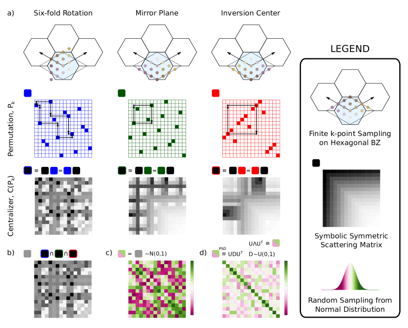
Figure 1: Schematic of procedure to generate physically-plausible collision operators randomly respecting crystal symmetries. (a) Finite states in the first Brillouin zone (legend) permuted by each crystal symmetry generator to a new state (top row). $N\times N$ permutation matrices corresponding to each symmetry generator (second row). Overlaid arrows show one cycle starting at state $i=2$. Starting with a symbolic symmetric scattering matrix (legend), we construct the centralizers for each permutation matrix (the basis elements of the vector space of matrices commuting with each permutation matrix, third row). (b) Maximal set of independent components identified by taking the union of the centralizers for each symmetry generator in (a). (c) Independent components assigned by sampling a random-normal distribution with zero mean and unit variance (legend). (d) Numeric matrix in (c) is spectrally-decomposed to extract symmetry-preserving eigenvectors, assigned random uniform eigenvalues ensuring positive-definiteness, and re-combined to form the collision operator.

Before describing the procedure to generate a physically-plausible state-resolved $R_{q}$ using arbitrary crystal symmetries, we note that in the case of an isotropic system we can identify the terms in the common dual relaxation-time approximation Lorentz (1905); Callaway (1959); de Jong and Molenkamp (1995) with carrier and momentum projection operators:

$$\Gamma[n]\approx \frac{1}{\tau_{\mathrm{mr}}}\left[-\delta n_{i}+\frac{1}{N}\sum_{j}\delta n_{j}\right]+$$

$$\frac{1}{\tau_{\mathrm{mc}}}\left[-\delta n_{i}+\frac{1}{N}\sum_{j}\delta n_{j}\left(1+2\bm{\hat{v}}_{j}\cdot\bm{\hat{v}}_{i}\right)\right].$$ (16)

Here, $\tau_{\mathrm{mr/mc}}$ refers to scalar momentum-relaxing/conserving lifetimes and $N$ is the total number of states.

Equation 16 can be written in the more illustrative form

$$\Gamma[n]\approx\frac{1}{\tau_{\mathrm{mr}}}\left[\mathbb{P}_{c}-1\right]\delta n+\frac{1}{\tau_{\mathrm{mc}}}\left[\mathbb{P}_{m}-1\right]\delta n,$$ (17)

where $\mathbb{P}_{c}$ and $\mathbb{P}_{m}$ are (isotropic) projectors which ensure carrier number and momentum conservation respectively.

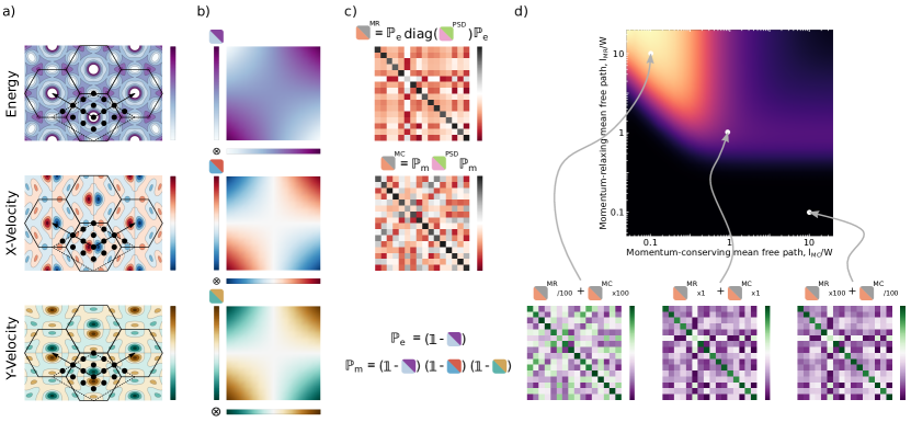
Figure 2: Schematic of procedure to project conserved quantities in physically-plausible collision operators. (a) Finite sampling of state-resolved quantities (energy and in-plane group velocities). (b) Projection operators constructed for each conserved quantity. (c) Momentum-relaxing and momentum-conserving collision operators constructed by projecting out the relevant quantities from the random numeric matrix from fig. 1d. (d) Linear combinations of momentum-conserving and momentum-relaxing collision operators from (c) scaled according to eqs. 24 and 25.

II.3 Physically Plausible State-Resolved Collision Operators

Despite the remarkable simplification of the BTE afforded by eq. 16, and its ubiquity in recent electron hydrodynamic studies Scaffidi et al. (2017); Sulpizio et al. (2019); Vool et al. (2021); Varnavides et al. (2022), it offers little insight into how the microscopic scattering details of the collision operator manifest in macroscopic observables. While eq. 8 allows us to go beyond the dual relaxation time approximation, it is often computationally intractable to compute the linearized collision matrix from first principles. Here, we propose a framework to generate collision operators randomly, constrained by crystal symmetries and conservation laws Hardy (1970), and scaled according to experimentally-accessible lifetimes:

1. We start by specifying the crystallographic point-group of the structure, $\mathcal{G}$, and sampling the first Brillouin zone (BZ) to obtain $N$ discrete states (fig. 1, legend). The number of states in the BZ sets our state-space resolution, and is only restricted to be divisible by the lengths of the orbits in the symmetry group of $\mathcal{S}[\mathcal{G}]$.

2. For each of the structure’s $k$ symmetry generators, we construct $N\times N$ permutation matrices $\mathcal{P}_{k}$ which map one discrete state to another (fig. 1a, middle row). Recall that permutation matrices are binary square matrices with exactly one non-zero entry in each row and each column satisfying $\mathcal{P}_{k}^{m}=I$, i.e. repeated $m$ applications, where $m$ is the the symmetry order, return the identity matrix (shown graphically by the black permutation paths).

3. Starting with a symmetric symbolic matrix (i.e. with $N\times\left(N+1\right)/2$ independent elements, fig. 1 legend), we construct the centralizer $\mathcal{C}$ for each $\mathcal{P}_{k}$. This is defined as the vector space of all matrices commuting with $\mathcal{P}_{k}$ (fig. 1a, bottom row):

   $$\mathcal{C}(\mathcal{P}_{k})=\left\{X\in M_{N\times N}(\mathbb{R})\;\middle|\;\mathcal{P}_{k}X=X\mathcal{P}_{k}\right\}.$$ (18)

   The maximal set of independent components is given by the intersection of these centralizers across permutation matrices (fig. 1b), which is solved as a recursive linear system since $\mathcal{P}_{k}$ are binary.

4. We sample these independent components from a normal distribution with zero mean and unit variance (fig. 1 legend), yielding a random scattering matrix $R_{0}$ which respects the system’s crystal symmetries (fig. 1c).

5. As constructed, $R_{0}$ may have unphysical (negative) eigenvalues. We therefore proceed by enforcing the matrix be positive semi-definite. This is done by spectrally decomposing the matrix and replacing its eigenvalues with random-uniform eigenvalues (fig. 1d):

   $$U\Lambda U^{T} =R_{0}$$

   $$R_{0}^{\mathrm{PSD}} =UDU^{T}\qquad\mathrm{s.t.}\;D\sim\mathcal{U}(0,1)$$ (19)

Steps (i-v) above generate a random positive semi-definite collision operator respecting the system’s crystal symmetries.

Next, we extend the procedure outlined above to project out conserved quantities of interest. In particular, we seek to generalize eq. 17 by constructing two state-resolved collision operators $R_{\mathrm{mr}}$ and $R_{\mathrm{mc}}$ where $R_{\mathrm{mr}}$ conserves carriers and $R_{\mathrm{mc}}$ conserves carriers and momentum. We then construct a family of collision operators with a tunable ratio of momentum-conserving to momentum-relaxing scattering according to:

$$R(\tau_{\mathrm{mc}},\tau_{\mathrm{mr}})=\tau_{\mathrm{mc}}^{-1}\frac{R_{\mathrm{mc}}}{\left|R_{\mathrm{mc}}\right|}+\tau_{\mathrm{mr}}^{-1}\frac{R_{\mathrm{mr}}}{\left|R_{\mathrm{mr}}\right|}.$$ (20)

Figure 3: (a) Fermi surface with square $(D_{4})$ symmetry (black solid line) parametrized in $N$ discrete steps (black points). Unit magnitude velocities are shown in red arrows. Swept over the Fermi wavevector angle, the velocities trace a self-intersecting curve (red dotted line), leading to strongly anisotropic velocity distributions (inset histogram). (b) Channel flow geometry of width $W$, with periodic and diffuse boundaries along the $\hat{x}$ and $\hat{y}$ directions respectively. (c) Current densities shown for the hydrodynamic (top-left), ballistic (top-right), porous (bottom-left), and diffusive (bottom-right) transport regime limits. The curvature obtained by fitting a parabola to the current distribution in the channel center is shown in the inset.

We start with $R_{0}^{\mathrm{PSD}}$ (fig. 1d) and perform the following steps:

1. Define the momentum projection operator as (fig. 2a-c)

   $$\mathbb{P}_{m}=\prod_{k}\left(I-u^{k}\otimes u^{k}\right),$$ (21)

   where $u^{k}$ is the orthonormal basis which spans the same $d+1$-dimensional space as the $\{\chi_{i}\}$ space spanned by the energy and $d$-components of the group-velocity and $d$ is the spatial dimension (e.g. in 2D $\chi_{i}=\left\{\epsilon_{i},v_{i}^{x},v_{i}^{y}\right\}$). Note that because we pin carriers to the Fermi surface conserving energy automatically also conserves carriers, but had we not done this we would additionally need to conserve carriers by including the vector $z_{i}=1$ in $\chi$ (i.e. each carrier contributes $1$ to the carrier count).

2. Construct the momentum-conserving collision operator by projecting $R_{0}^{\mathrm{PSD}}$ on both sides (fig. 2c)

   $$R_{\mathrm{mc}}=\mathbb{P}_{m}\,R_{0}^{\mathrm{PSD}}\,\mathbb{P}_{m}.$$ (22)

   Projection on the left ensures momentum conservation, and projection on the right ensures $R_{\mathrm{mc}}$ is symmetric. The resulting collision operator has $d+1$ zero eigenvalues and spectral radius $\sim$1.

3. In principle, the maximally momentum-relaxing collision operator is similarly given by defining the operator $\mathbb{Q}_{m}=I-\mathbb{P}_{m}$ to project $R_{0}^{\mathrm{PSD}}$ with on both sides. However, the resulting operator only has $d$ non-zero eigenvalues leading to a spectral radius of $N/2-1$. While this is physically permissible, it is numerically very challenging Varnavides et al. (2019). Instead, we approximate the momentum-relaxing collision operator using an anisotropic analogue of the first term in eq. 16 (fig. 2c):

   $$R_{\mathrm{mr}}=\mathbb{P}_{\epsilon}\,\mathrm{diag}\left(R_{0}^{\mathrm{PSD}}\right)\,\mathbb{P}_{\epsilon},$$ (23)

   where $\mathbb{P}_{\epsilon}$ is the energy projection operator. $R_{\mathrm{mr}}$ now has only one zero eigenvalue and a spectral radius of unity.

Steps (i-viii) above generate the two random positive semi-definite operators in eq. 20 respecting the system’s crystal symmetries and appropriate conservation laws. The only remaining steps are to specify appropriate normalizations $|R|$.

1. We normalize the momentum-conserving collision operator to have an average lifetime of unity by multiplying $R_{\rm mc}$ through by (fig. 2d)

   $$|R_{\mathrm{mc}}|^{-1}=\frac{1}{N}\left(R_{\mathrm{mc},ii}\right)^{-1}.$$ (24)

2. By contrast, we normalize the momentum-relaxing collision operator to have a Drude lifetime of unity by multiplying $R_{\rm mr}$ through by (fig. 2d, appendix A)

   $$|R_{\mathrm{mr}}|^{-1}=\frac{1}{Nv_{F}}\sqrt{\sum_{\alpha\beta}\left(v_{j}^{\alpha}\left(R_{\mathrm{mr}}\right)^{-1}_{ji}v_{i}^{\beta}\right)^{2}}.$$ (25)

Note that for an isotropic system, steps (i-x) fully-specify the collision operator, i.e. there are no independent components, exactly reproducing the dual relaxation-time approximation collision operator eqs. 16 and 17.

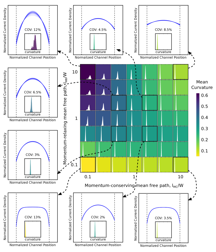
Figure 4: Current-density variability results for a system with square ($D_{4}$) symmetry. Distribution of curvatures for $K=100$ random collision operator instances on a grid of normalized momentum-conserving and momentum-relaxing mean free paths, using a common scale highlighting the increasing curvature variability in the hydrodynamic regime. Each grid tile’s background is color-coded according to its mean curvature. Callouts plot the $K=100$ normalized current densities for each random instance, for the four transport regime limits (top-right: ballistic, top-left: hydrodynamic, bottom-left: porous, bottom-right: diffusive), as well as four more experimentally-accessible transport regimes symmetric about $l_{\mathrm{mr}}=l_{\mathrm{mc}}=W$. Insets show zoomed-in curvature distributions, together with the distribution’s coefficient of variability $\mathrm{COV}(\%)=\sigma/\mu\times 100$.

III Results

III.1 Current Density Variability

We now apply the formalism developed in section II to investigate the sensitivity of hydrodynamic electron channel flow to the details of the collision operator. We restrict ourselves to scattering between states on the Fermi surface (fig. 3a) and work in a two-dimensional channel, with periodic and diffuse boundary conditions de Jong and Molenkamp (1995); Sulpizio et al. (2019); Vool et al. (2021) along the $\hat{x}$ and $\hat{y}$ directions respectively (fig. 3b). A weak electric field $E\hat{x}$ is applied to drive the current. We choose a unit-magnitude velocity normal to the Fermi surface, and fix the units such that a lifetime of $\tau=1$ corresponds to a mean-free path equal to the channel width. This allows us to parameterize our collision operators in the non-dimensionalized space of $\left(l_{\mathrm{mc}}/W,l_{\mathrm{mr}}/W\right)$, where $l_{\mathrm{mc/mr}}$ are the momentum-conserving/relaxing mean free paths, respectively, and $W$ is the width of the channel.

For each point in a grid of $\left(l_{\mathrm{mc}}/W,l_{\mathrm{mr}}/W\right)$, we generated $K=100$ random collision operators. For each collision operator we solve eq. 8 to obtain the spatially resolved carrier population $\delta n_{i}(\bm{r})$, from which we derive the current density profile. We then fit a parabola to the current density profile to obtain the current density curvature (fig. 3c).

We begin with a system with square ($D_{4}$) symmetry (fig. 4). Each square in the grid corresponds to one choice of $\left(l_{\mathrm{mc}}/W,l_{\mathrm{mr}}/W\right)$ and colored by the mean curvature of all $K=100$ collision operators we generated with those parameters.

We see increasing curvature towards long momentum-relaxing and short momentum-conserving mean-free paths, signalling the onset of hydrodynamics. This is consistent with the transport-regime diagrams characteristic of the dual relaxation-time approximation Sulpizio et al. (2019); Vool et al. (2021); Varnavides et al. (2022).

The distribution of curvatures is overlaid in white for each square, highlighting that the variability between samples is larger in the hydrodynamic regime (upper-left) than in the diffusive regime (lower-right) or ballistic (upper-right). This may also be seen in the current density plots surrounding the grid.

We use the coefficient of variability $\mathrm{COV}(\%)=\sigma/\mu\times 100$, where $\mu$ and $\sigma$ are the distribution’s mean and standard deviation respectively, as a normalized measure of variance and find that, even in the hydrodynamic regime, the macroscopic current density observable only exhibits a $\leq$12% variability between samples. If we instead restrict ourselves to the more experimentally-accessible regime of $l_{\mathrm{mr}}\sim l_{\mathrm{mc}}\sim W$ we find that the variability is on the order of $\sim$5%, which is smaller than typical experimental uncertainties.

We find that the current density profile is most sensitive to the details of the scattering processes in the hydrodynamic limit, though even there this sensitivity is minimal, and the current density profile is primarily a measure of the relative rates of momentum-conserving and momentum-relaxing scattering processes.

Finally, we illustrate the generality of our framework by investigating two additional crystal systems, those with hexagonal ($D_{6}$) and six-fold ($C_{6}$) symmetry. Figure 5 summarizes the results by plotting pairwise-comparisons between different symmetries in the different panels for one point in the $(l_{\mathrm{mc}}/W,l_{\mathrm{mr}}/W)$ grid, the experimentally-accessible regime $l_{\mathrm{mr}}=l_{\mathrm{mc}}=W$. Each panel shows the current density profiles. To understand the differences between these distributions we turn to the quantile-quantile plots (insets). Each quantile-quantile plot matches each percentile curvature of one symmetry with the corresponding percentile of the other. Importantly, in the inset of (fig. 5a) we see that the curvatures of $D_{6}$ are systematically higher than those of $D_{4}$, which results from the anisotropy of the Fermi velocity Varnavides et al. (2022).

III.2 Viscosity Tensor Variability

A common approach to avoid the computational cost of solving eq. 8 is to instead take the first moment of the BTE to recover the electronic Stokes equation Levitov and Falkovich (2016); Varnavides et al. (2020); Scaffidi et al. (2017):

$$\partial_{t}u_{\alpha}=\partial_{\beta}T^{(v)}_{\beta\alpha}-\partial_{\alpha}P-R_{\alpha\beta}u_{\beta}$$ (26)

where $u$ is the electron fluid velocity (current density), $P$ is the pressure (related to electrochemical potential $\Phi$ through $P=e\int_{n_{0}}^{n}\Phi(n^{\prime})dn^{\prime}\approx e(n-n_{0})\Phi$), $R_{\alpha\beta}$ is a positive semi-definite rank-2 tensor proportional to the momentum-relaxing rate, $T^{(v)}_{\alpha\beta}$ is the viscous contribution to the stress (momentum flux) tensor, and Greek letter subscripts correspond to cartesian directions. The stress is related to the fluid velocity to linear order by the rank-4 electronic viscosity tensor, $A_{\alpha\beta\gamma\zeta}$:

$$T^{(v)}_{\alpha\beta}=A_{\alpha\beta\gamma\zeta}\partial_{\zeta}u_{\gamma}.$$ (27)

As with all physical properties in crystals, the viscosity tensor is constrained by i) “intrinsic” tensor symmetries, ii) crystal symmetries, and iii) thermodynamic stability. Due to the rich landscape of viscous effects such as Hall-viscosity and vorticity coupling enabled by preferred directions inside crystals  Avron (1998); Rao and Bradlyn (2020); Epstein and Mandadapu (2020); Varnavides et al. (2020), the solution of eq. 26 hinges on accurate calculation of the viscosity tensor.

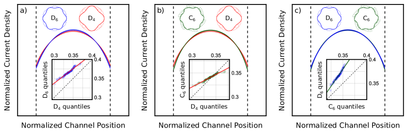
Figure 5: Comparison of normalized current-density profiles for different crystallographic point groups for $l_{\mathrm{mr}}=l_{\mathrm{mc}}=W$. (a) 95% confidence intervals for $K=100$ random instances for systems with square ($D_{4}$, red) and hexagonal ($D_{6}$, blue) crystal symmetries. Inset shows a QQ-plot of the hexagonal calculation’s curvature quantiles against those of the square calculation. The reasonable fit suggests the distributions have similar variance, with the rigid offset indicating the hexagonal calculation has larger curvatures. Similar comparison as in (a), comparing (b) a six-fold ($C_{6}$, green) system with a square ($D_{4}$, red) system and (c) a hexagonal ($D_{6}$, blue) system with a six-fold ($C_{6}$, green) system.

In Appendix B we derive a method to calculate the viscosity tensor given a collision operator. In this section we evaluate the viscosity and its variability using the same random collision operator instances from section III.1. Table 1 summarizes the normalized viscosity means and standard deviations using the same random collision operator instances as in section III.1. Note that our choice to produce symmetric collision operators in section II.3 implies microscopic reversibility and thus precludes any Hall-viscosity components. Similarly, the incompressibility condition we used in appendix B means that we cannot measure the components of the viscosity that couple to compression, i.e. we obtain $A_{ij11}=-A_{ij22}$. We see that the viscosity tensor varies substantially between collision operators of fixed $\tau_{\rm MR/MC}$, with coefficients of variability $>50\%$. This is in contrast to the minimal variation we saw in the current density profiles in section III.1, and indicates that the viscosity tensor is sensitive to the microscopic details of the collision operator.

IV Conclusions

We present a theoretical and computational formalism to generate physically plausible collision operators respecting a system’s crystal symmetries and conservation laws. We use this formalism to quantify the sensitivity of macroscopic observables to microscopic interaction details in electron hydrodynamics. We find that the detailed transition rates between electronic states produce small corrections, of order $\sim$10%, to current density profiles in 2D channel flow. Rather, the curvature in the middle of the channel is set primarily by the size of the geometry, and the ratio of momentum-relaxing to momentum-conserving lifetimes. This has several key implications.

First, for simple geometries such as channel flow, it should be possible to accurately predict the current density profile armed only with the knowledge of the momentum-relaxing and momentum-conserving lifetimes. As lifetime data are generally more experimentally accessible and readily predicted from first principles than collision operators, this represents a significant simplification to such calculations while retaining the full spatial and state resolution of the BTE. Conversely, this suggests that microscopic interaction details are difficult to probe with current density measurements since Kolkowitz et al. (2015); Andersen et al. (2019), at fixed lifetimes, the variance in current density profiles across random collision operator instances is small. More spatially-complex electronic flows, such as rotational flow in a Corbino disk geometry Varnavides et al. (2020) and vortices in a double chamber geometry Aharon-Steinberg et al. (2022), may fill this gap. Secondly, we find that the viscosity tensor – a key input parameter in modeling these electron fluids using the electronic Stokes equation Levitov and Falkovich (2016); Scaffidi et al. (2017); Varnavides et al. (2020) – is significantly more sensitive to the details of the collision operator, with variance across samples larger than 50%. Thus the action of viscosity on the channel flow resistance provides an experimental probe of the underlying scattering processes.

Taken together, our observations suggest several paths towards probing momentum-conserving interactions in electron fluids. First, spatially resolved current density measurements are a powerful tool to assess the regime of transport (namely, hydrodynamic or not) and the relative rates of momentum-conserving and momentum-relaxing scattering processes, but are not as informative on the details of those scattering processes. Secondly, viscosity measurements such as channel flow resistance and/or Corbino disk voltage drops Varnavides et al. (2020), which are only meaningful in the hydrodynamic limit, can probe the details of the collision operator. Thus the two work in conjunction: current density measurements allow one to identify a hydrodynamic system, and viscosity measurements allow one to probe the underlying scattering physics.

Finally, we note that our formalism for producing random collision operators can be readily adapted to other conserved quantities (for example spin), symmetries, and random distributions. Thus it provides a fast and adaptable tool for modelling scattering in a wide range of contexts.

Appendix A Drude Model Lifetime

Here we relate lifetimes in our formalism to those given by the Drude model of conductivity. The linearized steady state BTE with an electric field is given by

$$e\bm{v}_{i}\cdot\bm{E}\left(-\frac{dn_{0}}{d\epsilon}\right)_{i}=M_{ij}n_{j},$$ (28)

where $n_{0}$ is the Fermi-Dirac distribution, $\epsilon$ is energy, and $\bm{E}$ is the gradient of the electrochemical potential. We can solve for $n_{j}$ to find

$$n_{j}=M_{ji}^{-1}\left(e\bm{v}_{i}\cdot\bm{E}\left(-\frac{dn_{0}}{d\epsilon}\right)_{i}\right)$$ (29)

where $M_{ji}^{-1}$ is the pseudoinverse of $M_{ij}$.

The momentum and current density of carriers is given by

$$\bm{p} =m_{e}n_{i}\bm{v}_{i}$$ (30)

$$\bm{j} =en_{i}\bm{v}_{i}=\frac{e}{m_{e}}\bm{p}$$ (31)

Which we can relate to the electric field using the steady state distribution (equation 29):

$$\bm{j}=e^{2}\bm{v}_{j}M_{ji}^{-1}\bm{v}_{i}\cdot\bm{E}\left(-\frac{dn_{0}}{d\epsilon}\right)_{i}.$$ (32)

The conductivity tensor is then given by

$$\sigma_{\alpha\beta}=e^{2}v_{j}^{\alpha}M_{ji}^{-1}v_{i}^{\beta}\left(-\frac{dn_{0}}{d\epsilon}\right)_{i}.$$ (33)

At low temperatures $\frac{dn_{0}}{d\epsilon}$ restricts contributions to $\sigma$ to come from scattering near the Fermi surface. Restricting sums over $i$ and $j$ to run over states near the Fermi surface then we can replace $\frac{dn_{0}}{d\epsilon}$ with the density of states, $g$ :

$$\sigma_{\alpha\beta}=-\frac{e^{2}g}{N}\left(v_{j}^{\alpha}M_{ji}^{-1}v_{i}^{\beta}\right),$$ (34)

where $N$ is the number of states we sample on the Fermi surface. On a spherical Fermi surface with a quadratic dispersion relation this simplifies to:

$$\sigma_{\alpha\beta}=-\frac{ne^{2}}{m_{e}v_{F}^{2}N}\left(v_{j}^{\alpha}M_{ji}^{-1}v_{i}^{\beta}\right),$$ (35)

where $v_{F}$ is the Fermi velocity.

In the relaxation time approximation, $M_{ji}^{-1}=-\tau\delta_{ij}$, so

$$\sigma_{\alpha\beta}=\frac{ne^{2}\tau}{m_{e}}\sum_{i,\alpha}\frac{\left(v_{i}^{\alpha}\right)^{2}}{Nv_{F}^{2}}\delta_{\alpha\beta}=\frac{ne^{2}\tau}{m_{e}}\delta_{\alpha\beta},$$ (36)

which is we identify as the Drude conductivity. For systems outside relaxation time approximation then, we can instead ascribe a mean lifetime

$$\tau_{\rm MR}^{2}\equiv\frac{1}{Nv_{F}^{2}}\sum_{\alpha\beta}\left(v_{j}^{\alpha}M_{ji}^{-1}v_{i}^{\beta}\right)^{2},$$ (37)

where we’ve taken a Frobenius norm of the conductivity tensor to arrive at a scalar lifetime.

Hexagonal Viscosity Tensor, $A_{\alpha\beta\gamma\zeta}^{D_{6}}$		Square Viscosity Tensor, $A_{\alpha\beta\gamma\zeta}^{D_{4}}$
$\left(\begin{array}[]{cc}\left(\begin{array}[]{cc}0.35\pm 0.18&0.\\ 0.&-0.35\pm 0.18\\ \end{array}\right)&\left(\begin{array}[]{cc}0.&0.35\pm 0.18\\ 0.35\pm 0.18&0.\\ \end{array}\right)\\ \left(\begin{array}[]{cc}0.&0.35\pm 0.18\\ 0.35\pm 0.18&0.\\ \end{array}\right)&\left(\begin{array}[]{cc}-0.35\pm 0.18&0.\\ 0.&0.35\pm 0.18\\ \end{array}\right)\\ \end{array}\right)$		$\left(\begin{array}[]{cc}\left(\begin{array}[]{cc}0.17\pm 0.14&0.\\ 0.&-0.17\pm 0.14\\ \end{array}\right)&\left(\begin{array}[]{cc}0.&0.5\pm 0.4\\ 0.5\pm 0.4&0.\\ \end{array}\right)\\ \left(\begin{array}[]{cc}0.&0.5\pm 0.4\\ 0.5\pm 0.4&0.\\ \end{array}\right)&\left(\begin{array}[]{cc}-0.17\pm 0.14&0.\\ 0.&0.17\pm 0.14\\ \end{array}\right)\\ \end{array}\right)$

Table 1: 2D Viscosity tensors computed using $K=100$ random collision operator instances for hexagonal ($D_{6}$) and square ($D_{4}$) systems. Entries show the normalized mean $\pm$ standard deviation, using the normalization $|A|^{2}=A_{\alpha\beta\gamma\zeta}A_{\alpha\beta\gamma\zeta}=1$.

Appendix B Extracting Viscosities

In this section, we derive the viscosity tensor within the BTE framework introduced in section II.1 using a simple carrier distribution perturbation Simoncelli et al. (2020); Steinberg (1958).

We work in the limit of perfect momentum conservation, and begin with a perturbed carrier distribution of the form:

$$\delta n_{i,1}(\bm{r})=\bm{v}_{i}\cdot\bm{u}(\bm{r}),$$ (38)

where $u$ is a background drift velocity field with shears $\partial_{\zeta}u_{\gamma}$. Because collisions conserve momentum, $\delta n_{i,1}$ is a null eigenvector of the collision operator. As such, at steady-state, we must add an additional perturbation on top of eq. 38 to satisfy eq. 5:

$$-\bm{v}_{i}\cdot\nabla\left(\delta n_{i,1}+\delta n_{i,2}\right)=\frac{\partial\Gamma_{i}}{\partial n_{j}}\delta n_{j,2}.$$ (39)

Next, we assume $\bm{u}(\bm{r})$ has a constant gradient, and thus $-\bm{v}_{i}\cdot\nabla\delta n_{i,1}$ is spatially homogeneous. This means $\delta n_{i,2}$ is also spatially homogeneous, so we can solve for the perturbation $\delta n_{j,2}$ using the linear system:

$$-\bm{v}_{i}\cdot\nabla\delta n_{i,1}=\frac{\partial\Gamma_{i}}{\partial n_{j}}\delta n_{j,2}.$$ (40)

The stress tensor is then given by:

$$T^{(v)}_{\alpha\beta}=v_{i,\alpha}v_{i,\beta}\;\delta n_{j,2}.$$ (41)

This allows us to reconstruct the viscosity tensor $A_{\alpha\beta\gamma\zeta}$ by sampling eq. 41 for various shears $\delta_{\zeta}u_{\gamma}$.

A subtlety here is that in steady state we need to enforce carrier conservation, which for many systems amounts to requiring the flow be incompressible. To see this we sum the steady state linearized BTE eq. 5 over states and find

$$\sum_{i}\left(\frac{\partial\Gamma_{i}}{\partial n_{j}}+\delta_{ij}\bm{v}_{i}\cdot\nabla_{\bm{r}}\right)\delta n_{j}(\bm{r})=\sum_{i}S_{i},$$ (42)

If the source term $S$ conserves carriers then the right-hand side vanishes. Following the reasoning in Section II.2, we construct collision operators which also conserve carriers to find

$$\sum_{i}\bm{v}_{i}\cdot\nabla_{\bm{r}}\delta n_{i}(\bm{r})=0.$$ (43)

Since $\delta n_{i,2}$ is spatially uniform, this becomes

$$\sum_{i}\bm{v}_{i}\cdot\nabla_{\bm{r}}\delta n_{i,1}(\bm{r})=0.$$ (44)

Inserting eq. 38 and assuming the group velocities are spatially uniform we find

$$\sum_{i}{v}_{i}^{\alpha}v_{i}^{\beta}\partial_{\alpha}u_{\beta}=0.$$ (45)

For the systems we study here, with $D_{4}$, $D_{6}$, and $C_{6}$ symmetry this amounts to requiring that the flow be incompressible ($\nabla\cdot\bm{u}=0$), but for more general symmetries the constraint may be more complex. This incompressibility constraint fundamentally arises from carrier conservation and linearizing the collision operator: if we allowed nonlinear contributions to the collision operator we could obtain steady state flows with compression.

Our approach then is to construct $d^{2}-1$ orthogonal shear tensors with vanishing divergence. For example, in 2D we use:

$$\delta_{\zeta}u_{\gamma}=\left\{\begin{pmatrix}0&1\\ 0&0\end{pmatrix},\;\begin{pmatrix}0&0\\ 1&0\end{pmatrix},\;\begin{pmatrix}1&0\\ 0&-1\end{pmatrix}\right\}.$$ (46)

For each of these we solve eq. 40 to calculate the stress tensor eq. 41, and reconstruct the viscosity tensor as the linear map between these.

References

- Krishna Kumar et al. (2017) R. Krishna Kumar, D. A. Bandurin, F. M. D. Pellegrino, Y. Cao, A. Principi, H. Guo, G. Auton, M. Ben Shalom, L. A. Ponomarenko, G. Falkovich, K. Watanabe, T. Taniguchi, I. Grigorieva, L. Levitov, M. Polini, and A. Geim, Nature Physics 13, 1182 (2017).
- Sulpizio et al. (2019) J. A. Sulpizio, L. Ella, A. Rozen, J. Birkbeck, D. J. Perello, D. Dutta, M. Ben-Shalom, T. Taniguchi, K. Watanabe, T. Holder, R. Queiroz, A. Principi, A. Stern, T. Scaffidi, A. K. Geim, and S. Ilani, Nature 576, 75 (2019).
- Marguerite et al. (2019) A. Marguerite, J. Birkbeck, A. Aharon-Steinberg, D. Halbertal, K. Bagani, I. Marcus, Y. Myasoedov, A. K. Geim, D. J. Perello, and E. Zeldov, Nature 575, 628 (2019).
- Ku et al. (2020) M. J. H. Ku, T. X. Zhou, Q. Li, Y. J. Shin, J. K. Shi, C. Burch, L. E. Anderson, A. T. Pierce, Y. Xie, A. Hamo, U. Vool, H. Zhang, F. Casola, T. Taniguchi, K. Watanabe, M. M. Fogler, P. Kim, A. Yacoby, and R. L. Walsworth, Nature 583, 537 (2020).
- Jenkins et al. (2020) A. Jenkins, S. Baumann, H. Zhou, S. A. Meynell, D. Yang, K. Watanabe, T. Taniguchi, A. Lucas, A. F. Young, and A. C. B. Jayich, arXiv:2002.05065 (2020).
- Gurzhi (1968) R. N. Gurzhi, Soviet Physics Uspekhi 11, 255 (1968).
- Moll et al. (2016) P. J. Moll, P. Kushwaha, N. Nandi, B. Schmidt, and A. P. Mackenzie, Science 351, 1061 (2016).
- Gooth et al. (2018) J. Gooth, F. Menges, N. Kumar, V. Su, C. Shekhar, Y. Sun, U. Drechsler, R. Zierold, C. Felser, and B. Gotsmann, Nature Communications 9 (2018).
- Osterhoudt et al. (2021) G. B. Osterhoudt, Y. Wang, C. A. C. Garcia, V. M. Plisson, J. Gooth, C. Felser, P. Narang, and K. S. Burch, Phys. Rev. X 11, 011017 (2021).
- Vool et al. (2021) U. Vool, A. Hamo, G. Varnavides, Y. Wang, T. X. Zhou, N. Kumar, Y. Dovzhenko, Z. Qiu, C. A. C. Garcia, A. T. Pierce, J. Gooth, P. Anikeeva, C. Felser, P. Narang, and A. Yacoby, Nature Physics (2021), 10.1038/s41567-021-01341-w.
- Aharon-Steinberg et al. (2022) A. Aharon-Steinberg, T. Völkl, A. Kaplan, A. K. Pariari, I. Roy, T. Holder, Y. Wolf, A. Y. Meltzer, Y. Myasoedov, M. E. Huber, B. Yan, G. Falkovich, L. S. Levitov, M. Hücker, and E. Zeldov, (2022), arXiv:2202.02798 [cond-mat.mes-hall] .
- Varnavides et al. (2022) G. Varnavides, Y. Wang, P. J. W. Moll, P. Anikeeva, and P. Narang, Phys. Rev. Materials 6, 045002 (2022).
- Wang et al. (2021) Y. Wang, G. Varnavides, P. Anikeeva, J. Gooth, C. Felser, and P. Narang, (2021), arXiv:2109.00550 [cond-mat.mtrl-sci] .
- Mendoza et al. (2011) M. Mendoza, H. J. Herrmann, and S. Succi, Phys. Rev. Lett. 106, 156601 (2011).
- Levitov and Falkovich (2016) L. Levitov and G. Falkovich, Nature Physics 12, 672 (2016).
- Guo et al. (2017) H. Guo, E. Ilseven, G. Falkovich, and L. S. Levitov, Proceedings of the National Academy of Sciences 114, 3068 (2017), https://www.pnas.org/doi/pdf/10.1073/pnas.1612181114 .
- Varnavides et al. (2020) G. Varnavides, A. S. Jermyn, P. Anikeeva, C. Felser, and P. Narang, Nature communications 11, 1 (2020).
- Scaffidi et al. (2017) T. Scaffidi, N. Nandi, B. Schmidt, A. P. Mackenzie, and J. E. Moore, Phys. Rev. Lett. 118, 226601 (2017).
- Kiselev and Schmalian (2019) E. I. Kiselev and J. Schmalian, Phys. Rev. B 99, 035430 (2019).
- Govorov and Heremans (2004) A. O. Govorov and J. J. Heremans, Phys. Rev. Lett. 92, 026803 (2004).
- Cepellotti et al. (2015) A. Cepellotti, G. Fugallo, L. Paulatto, M. Lazzeri, F. Mauri, and N. Marzari, Nature Communications 6, 6400 (2015).
- Guo et al. (2016) H. Guo, E. Ilseven, G. Falkovich, and L. Levitov, (2016), 10.48550/ARXIV.1612.09239.
- Ledwith et al. (2019) P. J. Ledwith, H. Guo, and L. Levitov, Annals of Physics 411, 167913 (2019).
- Callaway (1959) J. Callaway, Phys. Rev. 113, 1046 (1959).
- Guyer and Krumhansl (1966) R. A. Guyer and J. A. Krumhansl, Phys. Rev. 148, 778 (1966).
- de Jong and Molenkamp (1995) M. J. M. de Jong and L. W. Molenkamp, Phys. Rev. B 51, 13389 (1995).
- Jermyn et al. (2019) A. S. Jermyn, G. Tagliabue, H. A. Atwater, W. A. Goddard, P. Narang, and R. Sundararaman, Phys. Rev. Materials 3, 075201 (2019).
- Varnavides et al. (2019) G. Varnavides, A. S. Jermyn, P. Anikeeva, and P. Narang, Phys. Rev. B 100, 115402 (2019).
- Romano (2020) G. Romano, (2020), arXiv:2002.08940 [cond-mat.mes-hall] .
- Coulter et al. (2018) J. Coulter, R. Sundararaman, and P. Narang, Phys. Rev. B 98, 115130 (2018).
- Garcia et al. (2021) C. A. C. Garcia, D. M. Nenno, G. Varnavides, and P. Narang, Phys. Rev. Materials 5, L091202 (2021).
- Lorentz (1905) H. A. Lorentz, Le mouvement des électrons dans les métaux (1905).
- Hardy (1970) R. J. Hardy, Phys. Rev. B 2, 1193 (1970).
- Avron (1998) J. E. Avron, Journal of Statistical Physics 92, 543 (1998).
- Rao and Bradlyn (2020) P. Rao and B. Bradlyn, Phys. Rev. X 10, 021005 (2020).
- Epstein and Mandadapu (2020) J. M. Epstein and K. K. Mandadapu, Phys. Rev. E 101, 052614 (2020).
- Kolkowitz et al. (2015) S. Kolkowitz, A. Safira, A. A. High, R. C. Devlin, S. Choi, Q. P. Unterreithmeier, D. Patterson, A. S. Zibrov, V. E. Manucharyan, H. Park, and M. D. Lukin, Science 347, 1129 (2015), https://www.science.org/doi/pdf/10.1126/science.aaa4298 .
- Andersen et al. (2019) T. I. Andersen, B. L. Dwyer, J. D. Sanchez-Yamagishi, J. F. Rodriguez-Nieva, K. Agarwal, K. Watanabe, T. Taniguchi, E. A. Demler, P. Kim, H. Park, and M. D. Lukin, Science 364, 154 (2019), https://www.science.org/doi/pdf/10.1126/science.aaw2104 .
- Simoncelli et al. (2020) M. Simoncelli, N. Marzari, and A. Cepellotti, Phys. Rev. X 10, 011019 (2020).
- Steinberg (1958) M. S. Steinberg, Phys. Rev. 109, 1486 (1958).