OptimizedDP: An Efficient, User-friendly Library For Optimal Control and Dynamic Programming

Abstract

This paper introduces OptimizedDP, a high-performance software library that solves time-dependent Hamilton-Jacobi partial differential equation (PDE), computes backward reachable sets with application in robotics, and contains value iterations algorithm implementation for continuous action-state space Markov Decision Process (MDP) while leveraging user-friendliness of Python for different problem specifications without sacrificing efficiency of the core computation. These algorithms are all based on dynamic programming, and hence can have bad execution runtime due to the large high-dimensional tabular arrays. Although there are existing toolboxes for level set methods that are used to solve the HJ PDE, our toolbox makes solving the PDE at higher dimensions possible as well as having an order of magnitude improvement in execution times compared to other toolboxes while keeping the interface easy to specify different dynamical systems description. Our toolbox is available online at https://github.com/SFU-MARS/optimized_dp.

Introduction

Dynamic programming based algorithms are crucial to many optimization problems. Despite its poor scalability due to exponential complexity, global optimal solutions to many control and optimization problems are only feasible via dynamic programming approach. Furthermore, dynamic programming also provides important reasoning about solutions of many complex algorithms.

Such algorithms that we would like to address in this work are continuous Markov Decision Process (MDP) value iteration algorithm, and level-set based algorithms that solve the HJ PDEs, whose solutions are crucial to guaranteeing safety of autonomous systems and the surrounding environment HJOverview . Our motivation for addressing the former in this toolbox is that none of the existing computational efficient machine learning libraries support value iteration with continuous state space and action. And our reasons for this toolbox to support solving HJ PDEs are discussed as follow.

As the numerical algorithm for solving the HJ PDE to obtain the Backward Reachable Tube (BRT) and Backward Reachable Set (BRS) defined in HJOverview is quite complex and involves many floating-point operations on a large dimensional grid, it takes significant effort and time to write the algorithm, prototype the system dynamics, waiting for output results (which can be hours/days), and validating the results. Scalability is probably the biggest downside of the framework but these aforementioned factors shy roboticists away more from applying reachability analysis to their research. To address these problems, there have been some toolboxes that were implemented: HelperOC as a wrapper of the level set toolbox ToolboxLS LsetToolbox1 , and the BEACLS library written in C++ and CUDA BEACLS . HelperOC and ToolboxLS are both written in MATLAB, which contains a rich set of visualizing plots and contours functions, and is user-friendly and quite powerful in prototyping mathematical models. However, this toolbox suffers from slow runtime with the MATLAB software package being proprietary. BEACLS, on the other hand, executes the level-set based numerical algorithm much faster than the MATLAB counterpart but has a very difficult interface to specify a problem setting and hence making the time spent on prototyping systems a bottleneck.

In this paper, we introduce our new toolbox that obtains the BRS and BRT much more efficiently which can assist researchers better in prototyping and applying optimal control algorithms to their system model. The advantages of our toolbox compared to the existing ones are the significant improvement of the execution runtime and the user-friendly interface for problem specifications in Python. The efficient implementation of the toolbox also allows reachability analysis to be done on dynamical systems of up to six dimensions, which was not the case previously.

The toolbox supports the following: level-set based algorithms solving the Hamilton-Jacobi PDEs to obtain BRT and BRS, one-shot computation of time-to-reach (TTR) value function TTR , and value iterations for Markov Decision Process (MDP) with continuous state space and action space. Our toolbox is implemented in Python and HeteroCL heterocl . The front-end used to initialize various problem formulation is written in Python while the backend implementing the algorithms are written in HeteroCL. HeteroCL is a python-based domain-specific language (DSL) that is based on Tensor Virtual Machine (TVM) chen2018tvm , a framework that optimizes deep learning programs as computation graph structures. HeteroCL is built on top of TVM that allows imperative programming in its syntax, which allows more flexibility in writing diverse algorithm implementations. Similar to TVM, HeteroCL decouples algorithm definitions from the scheduling transformations that can optimize the runtime of the programs. For our implementation, we attribute the considerable improvement in running time to the scheduling optimizing scheme available that we use and also the optimization done on graphs by the TVM framework. Our toolbox is available online at https://github.com/SFU-MARS/optimized_dp.

In the next few subsections, we will provide an overview of related software packages, optimizedDP’s software structure, features, description of the algorithms in the toolbox, and finally implementation details of those algorithms.

Related work

We are aware of other existing toolboxes that are most commonly used for solving HJ PDE:

ToolboxLS LsetToolbox1 is a library that contains many subroutines written in MATLAB for solving a variety of cases of an HJ PDE. HelperOC is a wrapper around ToolboxLS that utilizes these subroutines for convenient computation of BRT and BRS through solving the time-dependent HJ PDE. HelperOC contains many different examples of system dynamics used in BRT computation. In comparison with optimizedDP, ToolboxLS and HelperOC is more mature and contains more advanced numerical schemes to approximate derivatives and numerical integration as well as diverse MATLAB subroutines used for visualizing plots. One downside to ToolboxLS and HelperOC is that the toolbox can be quite slow for large problems and not possible for problems with systems that have higher than 4 dimensions. Another minor disadvantage of ToolboxLS is that it is written in MATLAB, a proprietary software package whose licenses have to be renewed yearly.

BEACLS is a library that contains implementations of all the features available in ToolboxLS and HelperOC in C++ and CUDA with support on GPU. This toolbox tries to solve the computational inefficiency issue that ToolboxLS faces. However, the biggest downside of this toolbox is that it’s quite hard to use due to the problem specification having to be written in C++.

Our toolbox optimizedDP introduced here is an ongoing effort that tries to combine the best features of the two toolboxes: codes that are easy to use, understand while keeping computations efficient. In addition, we are also aware of other software libraries for solving value iteration in MDP:

Markov Decision Process for Python is a software package written in Python that includes many algorithm implementations for MDP such as value iteration, policy iteration, relative value iteration, etc. However, the package does not support continuous state space and action space in value iteration. This package is available at https://pymdptoolbox.read thedocs.io/en/latest/ index.html.

POMDP JuliaMDP is a software package written in Julia that contains a variety of algorithm solvers for MDP and reinforcement learning algorithms such as Deep Q-learning, Monte Carlo Tree Search, etc. The package also contains many examples for different types of problem initialization and has an easy-to-use interface. But like Markov Decision Process for Python, the package does not support continuous state space and action space value iteration in MDP.

Overview of the software toolbox structure

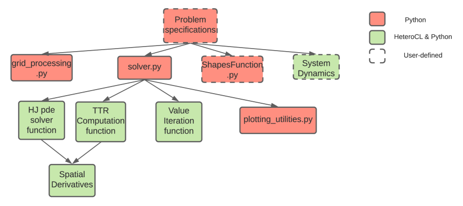
Figure 1: The overall structures of OptimizedDP. The red-colored files are written in Python and uses Numpy library for problem specifications, grid initialization, and plotting utilities. The green-colored files are written in a mix of HeteroCL and Python. The system dynamics file has to be provided by users and needs to be a Python object that contains problem parameters, and subroutines that determine optimal controls, optimal disturbances and compute the rate of change for each system state. These system object’s subroutines are then called by the rest of the green-colored files that provide implementations of the core algorithms.

The general structure of our toolbox is shown in Figure 1. To begin the computation, users first specify a problem specification file that imports the file solver.py, which contains definitions of APIs calls for three different types of computations. The problem specification file can be quite straightforward to users as it is mostly written with Python and Numpy libraries. To assist users in initializing their problem specifications, there are provided python libraries that include grid generations (file grid_processing.py), initialization of signed distance initial value function (file ShapesFunction.py). These functions could be extended or customized towards users’ needs, as long as the APIs are called correctly. The only HeteroCl part of the problem specifications is the system dynamics description, which is passed to the backend solvers to build a computational graph at the beginning.

The solver.py file maps the problem specification to the corresponding algorithm implementations. Each algorithm is implemented in HeteroCL which creates a computational graph of the algorithm and then returns an executable. The executables are used as a function to which parameters of the problem are passed. Once the results are computed and converted to a Numpy array, available visualization package libraries in Python can be used to display the result. To make visualization of high dimension array easier, the file plotting_utilities.py creates a wrapper around the plotly’s Isosurface function that can be called to visualize 3D value function representing various slices of the multidimensional result array. In addition, certain computation modules can be cross-used among different algorithms implementation. Specifically, the module spatial derivatives computation is both used in solving HJ PDE and computing TTR value function.

Features And Algorithms Supported

Continuous Markov Decision Process (MDP) & Value Iteration

Markov Decision Process is a model that is useful to study the optimal behavior of a target system in react to the change of external environments. An MDP is usually described by a tuple $(S,A,T,R,\gamma,H)$ where $S$ is the state space, $A$ is the action space, $T$ is the transition probability matrix, $\gamma$ is the discount factor and $H$ is the time horizon. The key assumption of MDP is that the next state transition of a system is only dependent on the current state and action. This assumption is described by the following relation

$$\mathbf{P}(S_{t+1}|S_{t},A_{t})=\mathbf{P}(S_{t+1}|S_{t},A_{t}...,S_{0},A_{0})$$ (1)

where $S_{t}\in S$, and $A_{t}\in A$. In MDP, the discounted return $G_{t}$ at time step $t$ is defined as:

$$G_{t}=R_{t+1}+\gamma R_{t+2}+\gamma^{2}R_{t+3}+...=\Sigma^{n}_{k=0}\gamma^{k}R_{t+k}$$ (2)

And the state value function $V_{\pi}(s)$ under a policy $\pi:S\rightarrow A$ is as follow

$$V_{\pi}(s)=E_{\pi}[G_{t}|S_{t}=s]=E_{\pi}[R_{t}+\gamma V_{\pi}(s^{\prime})|S_{t}=s]$$ (3)

In MDP, the objective of the target system is to act according to an optimal policy $\pi^{*}:S\rightarrow A$ that can maximize the expected rewards received at each state over time. The main goal in MDP is to discover $\pi^{*}$ along with the expected rewards received at every state. This objective and the basic properties of MDP are the backbone of all reinforcement learning algorithms.

Our toolbox provides an implementation of the value iteration algorithm for continuous state and action space (shown in Algorithm 1), which computes expected rewards $V_{\pi^{*}}(s)$ at every state given all the possible actions a state $s$ can take.

Algorithm 1 Continuous MDP - Value Iteration Algorithm

1:Discretize $S,A$

2:$V_{t=0}\leftarrow 0$

3:Repeat:

4:for  $s$ in $S$ do

5:     for  $a$ in $A$ do

6:         $Q(s,a)\leftarrow R(s,a)+\sum_{s^{\prime}}p(s^{\prime}|s,a)V_{t-1}(s^{\prime})$

7:         $V_{t+1}(s)\leftarrow max(V_{t+1}(s),Q(s,a))$

8:         $\Delta\leftarrow\absolutevalue{V_{t}(s)-V_{t+1}(s)}$

9:         If $\Delta<$ threshold:

10:               Break

11:     end for

12:end for

Note that on line 6 of algorithm 1, $(s^{\prime})$ is obtained by considering the nearest neighbour that is the closest discretized state on grid.

Time-dependent Hamilton-Jacobi (HJ) Partial Differential Equation (PDE)

Our toolbox supports numerical computation for solving two HJ PDEs. The first PDE, which is solved in order to obtain BRS and BRT defined in HJOverview , is as follow:

$$\begin{gathered}D_{s}\phi(z,s)+H(z,\nabla\phi(z,s))=0\\ H(z,\nabla\phi(z,s))=\min_{d(\cdot)}\max_{u(\cdot)}\nabla\phi(z,s)^{T}f(z,u,d)\\ \phi(z,0)=\phi_{0}(z),s\in[t,0]\end{gathered}$$ (4)

The algorithm based on level-set methods for solving the above equation is implemented as in algorithm 2.

Algorithm 2 Time-dependent HJ PDE algorithm

1:Initialize $\phi_{0}$

2:// Compute Hamiltonian term, max and min derivative

3:for  every grid point index i  do

4:     Compute $\nabla\phi(z,s)$

5:     $\displaystyle u_{opt}\leftarrow\arg\max_{u\in\mathbb{U}}\nabla\phi(z,s)^{\top}f(z,u)$

6:     $\dot{z}\leftarrow f(z,u_{opt})$

7:     $H_{i}\leftarrow\nabla\phi(z,s)^{\top}\dot{z}$

8:     $minD\leftarrow min(minD,\nabla\phi(z,s))$

9:     $maxD\leftarrow max(maxD,\nabla\phi(z,s))$

10:end for

11:// Compute artificial dissipation

12:for every grid point index i do

13:     $\alpha_{i}\leftarrow\max_{p\in[minD,maxD]}\absolutevalue{\dfrac{\partial H}{\partial p}}$

14:     $H_{i}\leftarrow H_{i}-\alpha_{i}\dfrac{D^{+}V_{i}-D^{-}V_{i}}{2}$

15:     $\alpha_{d}^{max}\leftarrow max(\alpha_{d}^{max},\alpha_{i})$

16:end for

17:// Compute integration time step

18:$\Delta t\leftarrow(\Sigma_{d=1}^{N}\dfrac{\absolutevalue{\alpha_{d}^{max}}}{\Delta z_{d}})^{-1}$

19:// First order Runge-Kutta (RK) integrator.

20:$V_{t+1}\leftarrow H\Delta{t}+V_{t}$

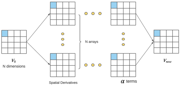
Figure 2: In LsetToolbox1 , each temporary variables are stored in multidimensional arrays. As we increase $N$, the number of dimensions, the number of temporary multi-dimensional array goes up linearly. If the depth of the computation is large, the total amount memory used for temporary variables will exceed system’s DRAM capabilities, limiting computations to small problems only.

Currently, the toolbox solves the above PDE for up to 6 dimensions. Although the toolbox developed by LsetToolbox1 supports an arbitrary number of dimensions through the usage of various operation tricks supported by MATLAB, each of the temporary variables such as spatial derivatives, system dynamics, etc. for each grid point is stored in a multidimensional array. This approach is not ideal for the performance of an already expensive computation in two ways (illustrated in Fig. 2 ). Firstly, the approach does introduce extra overhead of memory in the implementation. These redundant overheads increase linearly as we go up the dimensional ladder, which can limit the number of dimensions to which the algorithm can be performed. Secondly, each of the components for all grid points has to be computed before the final output, which results in bad cache locality for high-dimensional problems.

Figure 3: OptimizedDP’s implementation of algorithm 2 does not buffer temporary variables into multidimensional arrays. Instead, within each grid iteration, a grid point value in $V_{new}$ is directly computed.

Time-independent Hamilton-Jacobi (HJ) Partial Differential Equation (PDE)

In addition, optimizedDP provides an implementation of the Lax-Friedrich sweeping algorithm described in TTR (also shown in algorithm 3) for efficiently computing time-to-reach BRS without numerical integration. Given a target set $\mathcal{T}\subseteq\mathcal{R}^{n}$, the time-to-reach (TTR) function is defined as follow:

$$\phi(z)=\min_{d(\cdot)}\max_{u(\cdot)\in\mathbb{U}}\min\{t\mid z(t)\in\mathcal{T}\}$$ (5)

By dynamic programming principle, this TTR $\phi(z)$ can be obtained by solving the following HJI PDE:

$$\begin{gathered}H(z,\nabla\phi(z))=0\\ \phi(z)=0,z\in\mathcal{T}\\ H(z,\nabla\phi(z))=\min_{d(\cdot)}\max_{u(\cdot)}(-\nabla\phi(z)^{T}f(z,u,d)-1)\end{gathered}$$ (6)

The advantages of algorithm 3 compared to obtaining the TTR function through solving the time-dependent HJ PDE are less memory is required and the convergent result generally requires fewer iterations.

Algorithm 3 Lax-Friedrich sweeping algorithm for TTR

1:Initialize $\phi(z)\leftarrow 0$ for $z\in\mathcal{T}$ and $\phi(z)\leftarrow 100$ for $z\not\in\mathcal{T}$

2:while $\absolutevalue{\phi-\phi_{old}}<\epsilon$ do

3:     $\phi\leftarrow\phi_{old}$

4:     for  grid index i not in boundary do:

5:         Compute $\nabla\phi(z,s)$

6:         $\displaystyle u_{opt}\leftarrow\arg\max_{u\in\mathbb{U}}\nabla\phi(z,s)^{\top}f(z,u)$

7:         $\dot{z}\leftarrow f(z,u_{opt})$

8:         $H_{i}\leftarrow\nabla\phi(z,s)^{\top}\dot{z}$

9:         $\sigma\leftarrow\absolutevalue{\dfrac{\partial H}{\partial p}}$

10:         $c\leftarrow\frac{\Delta z}{\sigma}$

11:         $\phi_{i}^{new}\leftarrow c(-H_{i}+\sigma\frac{\phi_{i+1}+\phi_{i-1}}{2\Delta z})$

12:         $\phi_{i}\leftarrow min(\phi^{new}_{i},\phi_{i})$

13:     end for

14:     // Update the grid points at boundary

15:     $\phi^{new}_{1}\leftarrow min(max(2\phi_{2}-\phi_{3},\phi_{3}),\phi_{1})$

16:     $\phi^{new}_{N}\leftarrow min(max(2\phi_{N-1}-\phi_{N-2},\phi_{N-2}),\phi_{N})$

17:end while

Common Components and Features

Grid

Similar to the ToolboxLS LsetToolbox1 , our toolbox allows users to create a Cartesian grid, implemented as a Python object, by specifying the number of grid nodes, upper bound, and lower bound for each dimension, and periodic dimension. The ghost points at the boundary for non-periodic dimension, by default, are extrapolated based on the formula described in the file addGhostExtrapolate.m in ToolboxLS.

Initial Condition

To initialize different implicit surface shapes, we have implemented many initial conditions which represent shapes such as cylinders, spheres, and lower/upper planes. In addition, there are utility functions that operate on these geometry shapes such as union, intersection. All of these functions are written with Python and Numpy, and could be easily extended by users using the attribute grid.vs exposed by the grid object.

Time Integration

OptimizedDP provides the standard first-order accurate strong stability preserving (SSP) Runge-Kutta (RK) integrator. The maximum timestep used for integration is determined by the Courant–Friedrichs–Lewy (CFL) CFL condition.

Spatial Derivatives

Currently, OptimizedDP provides an implementation of derivatives approximation method that includes first order upwind approximation and second order accurate essentially non-oscillatory (ENO) ENO scheme.

Visualization

OptimizedDP provides an interface that helps visualize 3D isosurface of implicit surface for high dimensional systems. This interface allows users to specify the slice indices for higher dimensional systems and set the threshold value of isosurface for visualization. At its core, the interface calls the function Isosurface available in plotly library, which will show the isosurface plot in a browser. Users can also opt to use other software packages for visualization once the final result is obtained.

Implementation Details

We decided to implement each algorithm mentioned in the above section for every dimension separately, each with its own nested loop implementation. Even though this can be a tedious process for development, there are few advantages for this approach. First, we would like to keep the algorithm implementation descriptive, intuitive, and easy to be understood by users who are familiar with the algorithms. More importantly, we would like to optimize the computation using some of the schedule transformations available in HeteroCL without introducing extra redundancy and overhead in the code. Currently, the toolbox supports core algorithm implementations for up to 6 dimensions. In our experience, this is the limit beyond which tabular dynamic programming is no longer practical on a personal computer of maximum 32GB DRAM.

In this section, we are going to discuss in more detail the optimization techniques enabled in HeteroCL used in our implementations, and note that not all of them are applicable to all the algorithms implementation.

Cache-Aware Optimized (Algorithm 1, 2, 3)

This optimization applies to all of the algorithm implementations. One important factor that can have a substantial impact on the performance of a program when dealing with high dimensional arrays is memory locality. By knowing the memory layout of the N-dimensional array, our grid iterations follow this layout order which takes advantages of the cache spatial locality. To abide by Numpy’s memory layout, the implementations, by default, assign the highest dimension being the most inner loop and the lowest dimension being the most outer loop. Users can define their grid’s dimension order so as this nested loop order matches with the system dynamic’s data re-use pattern, which can potentially result in computation savings.

Figure 4: Nested loop order that follows the linear memory map will take advantage of the main memory’s spatial locality

Another technique that can take advantage of the temporal locality of the cache is blocking, which is not implemented by default since the blocking size that can speed up the computation on different machines vary differently. But this can be easily implemented by users as HeteroCL allows loop transformations such as loop splitting, reorder, etc. through transformative primitives (in a few lines of codes) without worrying about affecting the implementation’s accuracy.

Parallel threading (Algorithm 2)

One important characteristic of algorithm 2 is that each grid point, within the same iteration, can be computed independently, and therefore in parallel. Note that this parallelization of computation only applies to solve time-dependent HJ PDE equations, which can be beneficial to the acceleration of the computation greatly. In particular, each computation of algorithm 2 on a grid point can be assigned a thread to it (shown in Fig. 6). In HeteroCL, this could be done by applying the transformation primitive parallel to a loop computation as shown in Fig.5.

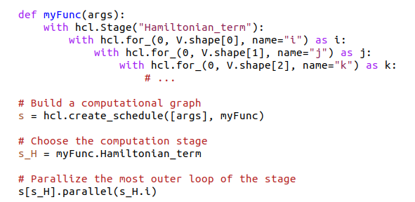
Figure 5: Computation can be parallelized by applying the parallel primitive

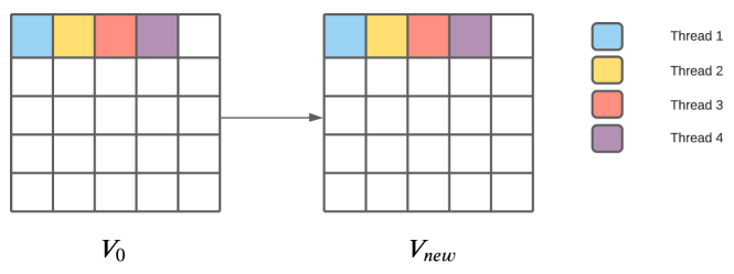
Figure 6: Each grid computation is assigned a thread for parallel computation

Under this primitive is an implementation of multi-threading in C++ provided by the TVM framework. The general idea of this multi-threading implementation is that there is a pool of threads where each thread pops and assigns itself a task (computation) from a task queue. The number of threads used is equal to the maximum number of hyper-threads available in the system. More details about the implementation are available online in the HeteroCL code base.

Alternating sweeping directions (Algorithm 1, 3)

This optimization is more algorithmic and less on the computer system level, and is applied to in-place value updating. In our toolbox, this approach is used in the implementation of value iteration algorithm and time-to-reach value function. The main idea is that the traversing directions on a multidimensional grid do not have to be fixed and can be alternated in different iterations until convergence. This technique has been shown to compute time-to-reach value function for 2D systems TTR .

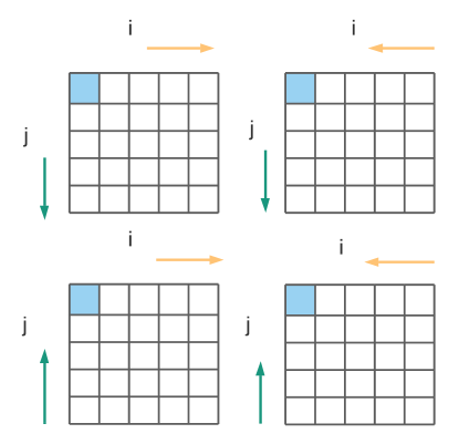
Figure 7: Each grid iteration can have alternating traversing direction for each dimension

The benefit of this optimization is that final value results would typically converge at a faster rate than iterating in a fixed direction. As we go up the dimensional ladder, the total number of different possible alternating directions increases exponentially. Because of that, for each implementation, we have a total of 8 different iterating directions.

Results

In this section, we first compare the performance of optmizedDP against the time-dependent HJ PDE implementation in ToolboxLS and BEACLS for various number of dimensions. These results are performed on a 16-thread Intel(R) Core(TM) i9-9900K CPU at 3.60GHz.

Table 1: Performance against ToolboxLS and HelperOC

Dimensions	3D	4D	5D	6D
Grid points	$100^{3}$	$60^{4}$	$40^{5}$	$25^{6}$
1st Order ENO scheme
OptimizedDP	$0.56$ seconds	$19$ seconds	$7$ seconds	$24$ hours
MATLAB LsetToolbox1	$3.8$ seconds	$196$ seconds	$223$ seconds	Not possible
Speedup	$\times$7	$\times$ 10	$\times$ 32	N/A
Maximum difference	1.4$\times 10^{-6}$	7.0$\times 10^{-6}$	1.4$\times 10^{-6}$	N/A
2nd Order ENO scheme
OptimizedDP	$0.7$ seconds	$23$ seconds	$10$ seconds	$1$ day
MATLAB	$12$ seconds	$678$ seconds	$754$ seconds	Not possible
Speedup	$\times$17	$\times$ 29	$\times$ 75.4	N/A
Maximum difference	0.037	0.25	0.1	N/A

Table 2: Performance against C++ BEACLS on CPU

Dimensions	3D	4D	5D
Grid points	$100^{3}$	$60^{4}$	$40^{5}$
1st Order ENO scheme
OptimizedDP	$0.56$ seconds	$19$ seconds	$0.72$ seconds
BEACLS	$1.5$ seconds	$244$ seconds	$4.84$ seconds
Speedup	$\times$3	$\times$ 13	$\times$ 6.7
2nd Order ENO scheme
OptimizedDP	$0.7$ seconds	$23$ seconds	$0.98$ seconds
BEACLS	$3$ seconds	$6420$ seconds	$8.28$ seconds
Speedup	$\times$4	$\times$ 279	$\times$ 8.44

For 3D system example, we compute BRT for the following canonical pairwise Dubins Car’s system dynamics:

$$\dot{x} =-v_{a}+v_{b}\cos\theta+ay$$ (7)

$$\dot{y} =v_{a}\sin\theta-ax$$

$$\dot{\theta} =b-a$$

where $x,y,\theta$ are the relative positions and heading, $v_{a}$ and $v_{b}$ are the evaders and pursuer’s velocity, $a$ and $b$ are the control input of the evader and pursuer respectively. 3D plots of the BRT are shown in Figure. 8.

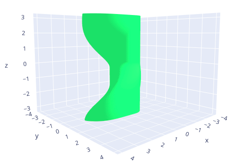
(a) Right side view (45 degree)

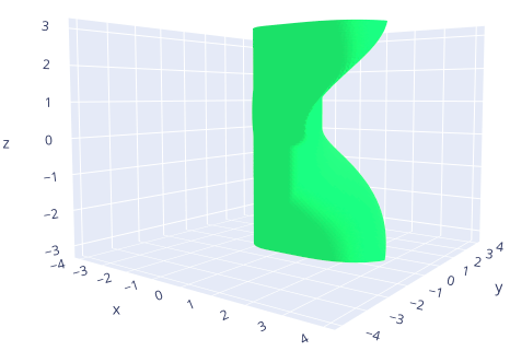
(b) Left side view

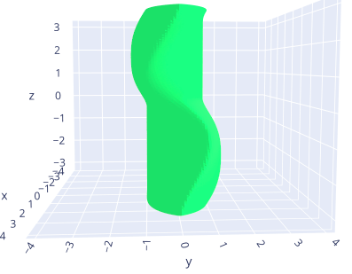
(c) Front view

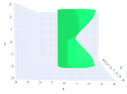
(d) Right side view (90 degree)

Figure 8: Sub-zero level set is the green surface shown in the plots

For 6D system example, we have the following system dynamics used for computing tracking error bound of an underwater vehicle with disturbances as defined in UnderwaterPaper :

$$\dot{x}_{\alpha} =u_{r}+{V}_{f,x}(x,z,t)+d_{x}-b_{x}$$

$$\dot{z}_{\alpha} =w_{r}+{V}_{f,z}(x,z,t)+d_{z}-b_{z}$$

$$\dot{u}_{r} =\frac{1}{m-X_{\dot{u}}}((\bar{m}-m)A_{f,x}(x,z,t)$$

$$\quad-(X_{u}+X_{\absolutevalue{u}u}\absolutevalue{u_{r}})u_{r}+T_{A})+d_{u}$$

$$\dot{w}_{r} =\frac{1}{m-Z_{\dot{w}}}((\bar{m}-m)A_{f,z}(x,z,t)$$

$$\quad-(-g(m-\bar{m}))-(Z_{w}+Z_{\absolutevalue{w}w}\absolutevalue{w_{r}})w_{r}$$

$$\quad+T_{B})+d_{w}$$ (8)

$$\dot{x} =u_{r}+{V}_{f,x}(x,z,t)+d_{x}$$

$$\dot{z} =w_{r}+{V}_{f,z}(x,z,t)+d_{z}$$

where $x,z$ denote the vehicle position, $u_{r},w_{r}$ represent relative velocities between vehicle and water flow, $x_{\alpha},z_{\alpha}$ denote relative position between tracker and planner. The control inputs are $T_{A},T_{B}$, planning inputs are $b_{x},b_{z}$, and disturbances are $d_{x},d_{z},d_{u},d_{w}$. The problem parameters are $m,\bar{m},X_{\dot{u}},Z_{\dot{w}},X_{u},X_{w}$, $X_{|u|u},Z_{|w|w}$. Contour plots of distances between the tracker and planner are shown in Figure 9.

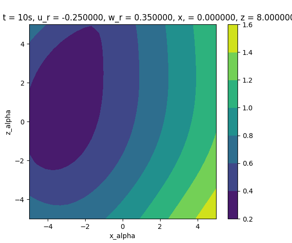
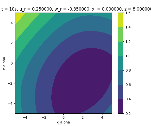
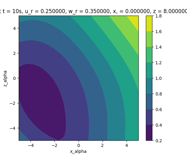
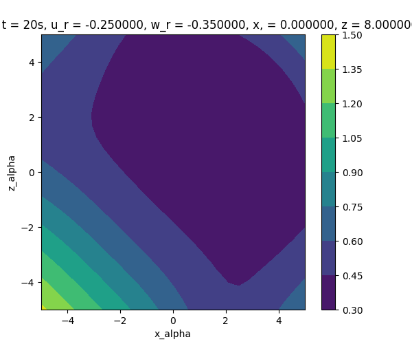
Figure 9: 2D contour plots of relative distances between the planner and tracker at different array indices and time. Each of the color on the vertical bar represents a distance value

Since there is no existing library that implements value iteration and algorithm 3 for time-independent HJ PDE, we only compare a version of value iteration written in pure Python, a commonly used language for reinforcement learning and MDP, with optimizedDP’s implementation.

Table 3: Value Iteration for 3D grid

Grid points	$25\times 25\times 9$	$40\times 40\times 20$	$50\times 50\times 30$
OptimizedDP	$0.17$ seconds	$0.45$ seconds	$0.98$ seconds
Python	$42.4$ seconds	$315$ seconds	$773$ seconds
Speedup	$\times$ 249	$\times$ 700	$\times$ 789

It can be observed that as the problem size increases, the gap in performance between optimizedDP and other existing implementations becomes larger. This proves that our toolbox is better for working with high-dimensional problems.

Limitation and future work

OptimizedDP toolbox is still a work in progress. Despite having better performance in terms of computational efficiency, optimizedDP is still missing some features that are available in other toolboxes. To make the toolbox more complete, we plan on adding new features to the toolbox such as higher order ENO scheme for derivatives approximation, more complex custom functions such as interpolation that can be used within a heteroCL graph.

References

- (1) Chen, M., Tomlin, C.J.: Hamilton–Jacobi Reachability: Some Recent Theoretical Advances and Applications in Unmanned Airspace Management. Annual Review of Control, Robotics, and Autonomous Systems 1(1), 333–358 (2018). DOI 10.1146/annurev-control-060117-104941. URL https://doi.org/10.1146/annurev-control-060117-104941
- (2) Chen, T., Moreau, T., Jiang, Z., Zheng, L., Yan, E., Cowan, M., Shen, H., Wang, L., Hu, Y., Ceze, L., Guestrin, C., Krishnamurthy, A.: Tvm: An automated end-to-end optimizing compiler for deep learning (2018)
- (3) Courant, R., Friedrichs, K., Lewy, H.: On the partial difference equations of mathematical physics. IBM Journal of Research and Development 11(2), 215–234 (1967). DOI 10.1147/rd.112.0215
- (4) Egorov, M., Sunberg, Z.N., Balaban, E., Wheeler, T.A., Gupta, J.K., Kochenderfer, M.J.: POMDPs.jl: A framework for sequential decision making under uncertainty. Journal of Machine Learning Research 18(26), 1–5 (2017). URL http://jmlr.org/papers/v18/16-300.html
- (5) Lai, Y.H., Chi, Y., Hu, Y., Wang, J., Yu, C.H., Zhou, Y., Cong, J., Zhang, Z.: Heterocl: A multi-paradigm programming infrastructure for software-defined reconfigurable computing. Int’l Symp. on Field-Programmable Gate Arrays (FPGA) (2019)
- (6) Mitchell, I.: The flexible, extensible and efficient toolbox of level set methods. J. Sci. Comput. 35, 300–329 (2008). DOI 10.1007/s10915-007-9174-4
- (7) Osher, S., Shu, C.W.: High-order essentially nonoscillatory schemes for hamilton–jacobi equations. Siam Journal on Numerical Analysis - SIAM J NUMER ANAL 28 (1991). DOI 10.1137/0728049
- (8) Siriya, S., Bui, M., Shriraman, A., Chen, M., Pu, Y.: Safety-guaranteed real-time trajectory planning for underwater vehicles in plane-progressive waves. In: 2020 59th IEEE Conference on Decision and Control (CDC), pp. 5249–5254 (2020). DOI 10.1109/CDC42340.2020.9303858
- (9) Tanabe, K., Chen, M.: Beacls (2021). Available at https://github.com/HJReachability/beacls
- (10) Yang, I., Becker-Weimann, S., Bissell, M.J., Tomlin, C.J.: One-shot computation of reachable sets for differential games. In: Proceedings of the 16th International Conference on Hybrid Systems: Computation and Control, HSCC ’13, p. 183–192. Association for Computing Machinery, New York, NY, USA (2013). DOI 10.1145/2461328.2461359. URL https://doi.org/10.1145/2461328.2461359