Hadamard and boundary conditions for the Big Bang quantum vacuum

Abstract

General relativity predicts final-type singularities inside black holes, as well as a cosmological initial-type singularity. Cosmic censorship protects external observers from black hole singularities, while Penrose’s Weyl curvature hypothesis protects the smoothness of the initial (Big Bang) singularity. We discuss a simple realization of the Weyl curvature hypothesis by assuming a very early radiation-dominated universe and analytically extending the expansion factor to negative values of conformal time. We impose time-reversal conditions at the Big Bang to characterize a natural set of preferred vacuum states for quantized matter fields. We implement the prescription of States of Low Energy constructed around the Big Bang obtaining Hadamard states. We also explore the physical implications of these vacua for cosmological dark matter production.

1 Introduction

The Weyl curvature hypothesis introduced by Penrose [1] is a natural and well-motivated way to smooth the Big Bang initial singularity. It can be regarded as complementary to Penrose’s cosmic censorship hypothesis [2], which protects the outside world from singularities that are predicted inside black holes.

The simplest way to enforce the Weyl curvature hypothesis, and to do so in a way that is consistent with observations, is through a Friedmann-Lemaître-Robertson-Walker (FLRW) geometry for spacetime [3]. Furthermore, as we go back in time the expansion factor $a(\tau)$ behaves in a very simple way $a(\tau)\propto\tau$, with respect to the conformal time $\tau$. This makes also natural to analytically extend to negative values the conformal time parameter [4], somewhat mimicking a bouncing geometry at the Big Bang. The advantage of this picture is that one can easily construct a well-defined vacuum state $|0_{-}\rangle$ at $\tau\to-\infty$. This vacuum state is then perceived as a collection of real particles at $\tau\to+\infty$. The absence of real particles at $\tau\to+\infty$ defines the vacuum $|0_{+}\rangle$. This is an example of gravitation particle creation, as originally established in [5, 6, 7]. Here we want to emphasize instead the emergent symmetry of the metric

$$ds^{2}\propto\tau^{2}(d\tau^{2}-d\vec{x}^{2})\,,$$ (1)

under the transformation

$$T:\tau\to-\tau\ .$$ (2)

This time-reversal symmetry has been pushed forward in [8, 9]. The vacuum state proposed in these references is the $T$-invariant linear combination $|0_{T}\rangle\propto|0_{+}\rangle+|0_{-}\rangle$. The corresponding particle production spectra at late times for both $|0_{-}\rangle$ and $|0_{T}\rangle$ is the same for large momenta, a decaying exponential, essentially describing thermal radiation.

In this work we analyze the issue of how to construct a vacuum state around the Big Bang $\tau\sim 0$. We note that, the selection of a preferred vacuum in the above-mentioned approaches is based on the asymptotic behaviour at $\tau\sim-\infty$, or $\tau\sim\pm\infty$. These vacua trivially satisfy the so-called Hadamard condition since they are constructed in the asymptotic regimes of the scale factor, for which the Hubble rate tends to zero. We recall that an admissible physical state in curved spacetime should have a short-distance behaviour similar to the vacuum in Minkowski space. We refer to this non-trivial property the Hadamard condition [10]. In an expanding universe this requirement was first established in momentum space and referred as the adiabatic condition [11]. In contrast, the construction of sensible vacuum states around $\tau\sim 0$, is more involved.

Selecting initial data to define the vacuum in a rapidly changing region of the spacetime, as is the case for the Big Bang, does not usually render a physically admissible quantum state in the ultraviolet. However, this non-trivial issue can be satisfactorily sorted out by using the states of low energy prescription [12, 13]. In this approach, the vacuum is defined as the state that minimizes the energy density smeared over a temporal window. The resulting state depends on the specific window function used and has been checked to satisfy the so-called Hadamard condition.

However, obtaining analytical expressions for the vacuum solutions that are also Hadamard is highly complicated around the Big Bang, even for states of low energy. Nevertheless, one can construct approximate Hadamard states that renders a finite $\langle T_{ab}\rangle$ after renormalization, and can be used to study particle creation and backreaction effects in semiclassical gravity. In this context, we analyze the possible approximated Hadamard vacuum states that can be defined around the Big Bang.

We consider two main applications of the above formalism in the context of gravitation particle production. One is the possible creation of gravitons in a radiation-dominated spacetime. If the vacuum is assumed to be constructed from the conformal modes, the predicted particle creation is exactly zero. This is the usual viewpoint. However, if the vacuum is a state of low energy at the Big Bang a non-trivial creation of (primordial) gravitons is allowed. Therefore, the inflationary paradigm is not the unique scenario to create gravitons. A second application, motivated here by conformal invariance, is the estimation of the mass for a right-handed sterile neutrino as a dark matter candidate. The sterile neutrino is assumed to be decoupled from the other particles of the Standard Model and the production mechanism is gravitational particle creation.

2 CPT-invariant vacuum states for scalar fields at the Big Bang: the Hadamard condition

In this section, we introduce the problem under consideration by considering a massive scalar field $\phi$ propagating in a flat FLRW spacetime (1) with a scale factor of the form $a(\tau)\propto\tau$, which corresponds to radiation-dominated universe. The coupling to the curvature $\xi R\phi^{2}$ is assumed to be generic. It is convenient to expand the quantized field in usual Fourier modes

$$\phi(\tau,\vec{x})=\int\frac{d^{3}k}{\sqrt{2(2\pi)^{3}}}\left(A_{\vec{k}}e^{i\vec{k}\vec{x}}\phi_{k}(\tau)+A_{\vec{k}}^{\dagger}e^{-i\vec{k}\vec{x}}\phi_{k}^{*}(\tau)\right)\ ,$$ (3)

where the creation and annihilation operators satisfy the usual commutation relations. For our purposes it is convenient to work with the rescaled Weyl modes $\varphi_{k}(\tau)\equiv a(\tau)\phi_{k}(\tau)$. The field equation implies ($ma=\gamma\tau$)

$$\varphi_{k}^{\prime\prime}+(k^{2}+\gamma^{2}\tau^{2})\varphi_{k}=0\ ,$$ (4)

and normalization condition $\varphi_{k}\varphi^{\prime}{}^{*}_{k}-\varphi_{k}^{\prime}\varphi_{k}^{*}=2i$. The general solution of (4) can be expressed in terms of parabolic cylindrical functions $D_{\nu}(z)$ [14]

$$\varphi_{k}(\tau)=\frac{1}{(2\gamma)^{1/4}}\Big{[}C_{k,1}\,D_{-\frac{1}{2}-2i\kappa}\big{(}e^{i\tfrac{\pi}{4}}\sqrt{2\gamma}\,\tau\big{)}+C_{k,2}\,D_{-\frac{1}{2}+2i\kappa}\big{(}e^{i\frac{3\pi}{4}}\sqrt{2\gamma}\,\tau\big{)}\Big{]}\,,$$ (5)

where $\kappa=\frac{k^{2}}{4\gamma}$. Any choice of $k$-functions $C_{k,1}$ and $C_{k,2}$ defines a set of modes characterizing a given vacuum state.

One can reduce the freedom in choosing a vacuum by exploiting the time-reversal symmetry $T:\tau\to-\tau$ of the background $ds^{2}\propto\tau^{2}(d\tau^{2}-d\vec{x}^{2}$). Since our scalar field theory is trivially invariant under parity ($P$) and charge conjugation ($C$) we can impose, more generally, CPT invariance. This means $CPT\varphi(x)(CPT)^{-1}=\varphi(-x)^{\dagger}$. The condition for a CPT-invariant vacuum state takes a very simple form on the time-dependent part of scalar field modes

$$\varphi_{k}(-\tau)=\varphi_{k}^{*}(\tau)\ .$$ (6)

Using standard properties of the parabolic cylindrical functions it can be easily shown that in terms of the general solution (5), the condition above implies $C_{k,1}=C_{k,2}^{*}$. For our purposes it is convenient to characterize the CPT-invariant condition at $\tau=0$. We easily find

$$\varphi_{k}(0)=\varphi_{k}^{*}(0)\,,\qquad\varphi_{k}^{\prime}(0)=-\varphi_{k}^{*\prime}(0)\,.$$ (7)

The general solution with the above constraints and the normalization condition can be parametrized as

$$\varphi_{k}(0)=\frac{1}{\sqrt{k}}e^{\theta_{k}}\,,\qquad\varphi_{k}^{\prime}(0)=-i\sqrt{k}\,e^{-\theta_{k}}\ ,$$ (8)

where $\theta_{k}$ is an arbitrary real function. In summary, the CPT requirement reduces the space of possible vacuum states to a family of states characterized by the hyperbolic initial ($\tau=0$) phase $\theta_{k}$. In terms of this parameter, the functions $C_{k,1}$ and $C_{k,2}$ read

$$C_{k,1}=2^{i\kappa}\sqrt{\pi}e^{\pi\kappa}\Bigg{(}\frac{e^{-\frac{i\pi}{4}}e^{\theta_{k}}}{\kappa^{\frac{1}{4}}\Gamma(\frac{1}{4}-i\kappa)}+\frac{i\,\kappa^{\frac{1}{4}}e^{-\theta_{k}}}{\Gamma(\frac{3}{4}-i\kappa)}\Bigg{)}\,,$$ (9)

and $C_{k,2}=C_{k,1}^{*}$.

The choice of the vacuum $|0\rangle$ has been then reduced to select a preferred function $\theta_{k}$. This can be interpreted as giving initial data at $\tau=0$. Before entering into a detailed discussion of how to single out a preferred vacuum it is convenient to analyze the particle production experienced by late-times observers.

2.1 Particle production and the choice of $\theta_{k}$

For each choice of an initial vacuum state $|0\rangle$ we have a different prediction for the particle creation spectrum at late times. Particles are defined at $\tau\to+\infty$ as excitations of the out-vacuum $|0_{+}\rangle$. The particle production rate can be obtained by the frequency-mixing approach [5]. In our case we find the following expression for the average density number of created particles in the mode $\vec{k}$

$$n_{k}\equiv|\beta_{k}|^{2}=-\frac{1}{2}+\frac{e^{-\pi\kappa}\cosh{(2\pi\kappa)}}{4\pi}\Bigg{(}e^{-2\theta_{k}}\,\kappa^{\frac{1}{2}}\,|\Gamma(\tfrac{1}{4}+i\kappa)|^{2}+e^{2\theta_{k}}\,\kappa^{-\frac{1}{2}}\,|\Gamma(\tfrac{3}{4}+i\kappa)|^{2}\Bigg{)},$$ (10)

where $\beta_{k}$ is one of the Bogoliubov coefficients. The number of created particles is minimized when (for more details see [13])

$$\theta_{k}^{late}=\frac{1}{4}\ln\Big{(}\frac{\kappa\cosh{(2\pi\kappa)}}{2\pi^{2}}|\Gamma(\tfrac{1}{4}+i\kappa)|^{4}\Big{)}\,.$$ (11)

In this case we obtain

$$n_{k}=\frac{1}{2}\left(\sqrt{1+e^{-4\pi\kappa}}-1\right)\,.$$ (12)

For large $k$ it has an exponential decay $n_{k}\sim e^{-\frac{\pi k^{2}}{\gamma}}$. We can regard (11) as an equivalent characterization of the preferred CPT-invariant vacuum proposed in [9, 8], namely, $|0_{T}\rangle\propto|0_{+}\rangle+|0_{-}\rangle$. We note that this vacuum also minimizes the energy density in the asymptotic regions $\tau\to\pm\infty$

$$\rho_{k}(\tau)\sim\omega_{k}|\beta_{k}|^{2}\ .$$ (13)

An alternative choice for the vacuum is simply the minimal choice $\theta_{k}=0$. It corresponds to the conformally invariant solution at $\tau\to 0$ as the equation of motion (4) suggests

$$\varphi_{k}\sim\frac{1}{\sqrt{k}}e^{-ik\tau}\ .$$ (14)

Furthermore, this choice minimizes the energy density at $\tau=0$ for $\xi=1/6$. In this case, we have

$$\rho_{k}(\tau)\sim\frac{k}{a^{4}}\cosh(2\theta_{k})\,.$$ (15)

For this choice and for large-$k$, the particle number behaves as

$$n_{k}\sim k^{-8}\,.$$ (16)

2.2 Ultraviolet regularity and the Hadamard condition

For a quantum state $|0\rangle$ to be admitted as physically acceptable we should demand it to be ultraviolet regular. This means that the high-energy behaviour of the state must approach the behaviour of Minkowski space at a rate such that, at least, basic composite operators, as the stress-energy tensor, can be renormalized. This is a necessary condition to properly study the semiclassical Einstein equations. Therefore, it is natural to require the renormalized form of $\langle 0|T_{\mu\nu}|0\rangle_{ren}$ to be well-defined. Since the renormalization subtractions in evaluating $\langle 0|T_{\mu\nu}|0\rangle_{ren}$ are essentially unique (up to finite counterterms), the ultraviolet behaviour of the modes must be compatible with the subtractions.

The mode decomposition (3) allows us to write the formal vacuum expectation values of the stress-energy tensor as a sum over modes

$$\langle T_{\mu\nu}\rangle=\int d^{3}k\ T_{\mu\nu}(\vec{k},\tau)\ .$$ (17)

A very useful renormalization scheme, which works in momentum space and does not depend on an explicit regulator, was introduced in [15, 16, 17, 18]. It involves a subtraction algorithm directly for the integrand in (17). The method is based on the adiabatic WKB-type expansion of the field modes

$$\varphi_{k}(\tau)\sim\frac{1}{\sqrt{W_{k}(\tau)}}e^{-i\int^{\tau}W_{k}(\tau^{\prime})d\tau^{\prime}}\ ,$$ (18)

where

$$W_{k}=\omega_{k}+\omega_{k}^{(2)}+\omega_{k}^{(4)}+\cdots\ ,$$ (19)

with $\omega_{k}=\sqrt{k^{2}+m^{2}a^{2}}$, and $\omega_{k}^{(n)}$ is the $n$-order term in a systematic adiabatic expansion. The adiabatic order is fixed by the number of $\tau$-derivatives of the scale factor $a(\tau)$. The above expansion of the modes is translated to an adiabatic expansion of $T_{\mu\nu}(\vec{k},\tau)$. This operation allows to extract from the integrand $T_{\mu\nu}(\vec{k},\tau)$ the divergent part of the overall integral (17). Therefore, one can write

$$\langle T_{\mu\nu}\rangle_{ren}=\int d^{3}k\ [T_{\mu\nu}(\vec{k},\tau)-T^{N-ad}_{\mu\nu}(\vec{k},\tau)]\ ,$$ (20)

where $N$ is the adiabatic order required to cancel the UV divergences of the integral (17). $T^{N-ad}_{\mu\nu}(\vec{k},\tau)$ is the associate adiabatic expansion of $T_{\mu\nu}(\vec{k},\tau)$ at order $N$. We note that $N$ can be regarded as the degree of divergence of (17). For the stress-energy tensor $N=4$ (in four spacetime dimensions). Since $\nabla^{\mu}T^{N-ad}_{\mu\nu}(\vec{k},\tau)=0$, the subtractions constructed this way preserve the covariant conservation of the renormalized stress-energy tensor. The adiabatic subtraction method can also be regarded as a version of the general DeWitt-Schwinger renormalization method when the spatial translations symmetry of the background is assumed [19]. More details can be found in [11, 20].

Since the subtractions $T^{N-ad}_{\mu\nu}(\vec{k},\tau)$ are essentially fixed, the major point now is to restrict the field modes involved in $T_{\mu\nu}(\vec{k},\tau)$, defining $|0\rangle$, such that $\langle 0|T_{\mu\nu}|0\rangle_{ren}$ be convergent. To this end, and in the context of our analysis, it is useful to evaluate the complete adiabatic expansion of the modes (18) at $\tau=0$. We get

$$\varphi_{k}(0)\sim\frac{1}{\sqrt{k}}+\frac{\gamma^{2}}{8\,k^{9/2}}+\frac{41\gamma^{4}}{128\,k^{17/2}}+\cdots\,.$$ (21)

From this we infer the asymptotic expansion of $\theta_{k}$

$$\theta_{k}\sim\frac{\gamma^{2}}{8k^{4}}+\frac{5\gamma^{4}}{16k^{8}}+\frac{61\gamma^{6}}{24k^{12}}+\cdots\,.$$ (22)

The set of vacuum states that fits the above large $k$ expansion up to a given order can be generically referred to as adiabatic vacuum states of finite order. The above adiabatic condition at all orders [generically (18), or (22) in this specific case] is equivalent to the Hadamard condition, as shown in [21].

A consequence of having a vacuum of infinite adiabatic order is that the number density of created particles in the mode $\vec{k}$ (i.e., $n_{k}$) with respect to the out-vacuum (which is also of infinite adiabatic order) decays faster than any power $k^{-N}$ for large $k$. Typically, an exponential decay. This very smooth behaviour of the field modes characterizing $|0\rangle$ ensures not only the ultraviolet convergence of the expectation values of the (renormalized) stress-energy tensor $\langle 0|T_{\mu\nu}|0\rangle_{ren}$, but also fluctuations of it. Furthermore, all polynomial functions of the stress-energy tensor, or the existence of Wick polynomials of arbitrary order of the field, require the Hadamard condition [22, 23, 24]. In contrast, for a vacuum of a finite adiabatic order the decay is a power-law. If we choose $\theta_{k}$ different from (22) we get these kind of vacua. For instance, choosing $\theta_{k}=0$ (zero adiabatic order) we find [25] $n_{k}\sim k^{-8}$. Furthermore, for $\theta_{k}\sim 1/k^{4}$ we also get $n_{k}\sim k^{-8}$, except for the case $\theta_{k}=\gamma^{2}/(8k^{4})$, for which $n_{k}\sim k^{-16}$. This behaviour ensures the UV convergence of the total number density of created particles,

$$\int\frac{d^{3}k}{(2\pi a)^{3}}n_{k}\ <+\infty\ .$$ (23)

In contrast, for $\theta_{k}\sim 1/k$ we get $n_{k}\sim k^{-2}$ and the integral evaluating the total number density is divergent.

It is less clear whether the convergence of (23) is enough to ensure the UV convergence of the most relevant quantities such as the energy density and pressure $\langle 0|T_{\mu\nu}|0\rangle_{ren}$. In Ref. [25] it has been analyzed this issue for the minimal solution $\theta_{k}=0$. Analyzing the ultraviolet behaviour of the stress-energy tensor for a general $\theta_{k}$ (see A for more details), we have found that to ensure its renormalizability, the asymptotic behaviour of $\theta_{k}$ should be

$$\theta_{k}\sim 0+\mathcal{O}\left(\frac{1}{k^{n}}\right),\ n>3\,.$$ (24)

3 States of low energy

In general spacetimes, a natural procedure to select and construct a preferred Hadamard vacuum state (i.e. a state of infinite adiabatic order) is not available. For FLRW spacetimes the problem is somewhat alleviated, due to the existence of isometries, and the construction of exact Hadamard states is possible [12]. These states are defined by minimizing the energy density after averaging with a temporal window function in a smooth region, no matter how short. If the window function shrinks to a point, we recover the traditional method of instantaneous diagonalization of the Hamiltonian, which produced states that are not Hadamard. The analysis of [12, 26] was only given for scalar fields (minimally coupled to the curvature). A more general survey, including spin-$\frac{1}{2}$ fields has been given in [13]. Here we will briefly review the construction for minimally coupled scalar fields and connect with the examples presented above.

The starting point is to selected a fiducial set of normalized modes $\phi_{k}(\tau)$. They are related to the Weyl modes of the previous section by $\varphi_{k}=a\,\phi_{k}$. We can choose them by convenience. One can parametrize a general set of modes $T_{k}(\tau)$ in the form

$$T_{k}(\tau)=\lambda_{k}\phi_{k}(\tau)+\mu_{k}\phi_{k}^{*}(\tau)\ ,$$ (25)

where $\lambda_{k}$ and $\mu_{k}$ are complex numbers that must obey $|\lambda_{k}|^{2}-|\mu_{k}|^{2}=1$. The goal now is to find for which values of $\lambda_{k}$ and $\mu_{k}$ the smeared energy density is minimal. It is given by

$$\mathcal{E}_{k}[f] := \int\text{d}\tau\,\sqrt{|g|}\,f^{2}\,\rho_{k}\,,$$ (26)

where $f^{2}(\tau)$ characterizes the window function and $\rho_{k}(\tau)$ is given by ($\omega^{2}=k^{2}+m^{2}a^{2}$)

$$\rho_{k}(\tau)=\frac{1}{4a^{2}}\left(|T^{\prime}_{k}|^{2}+\omega^{2}|T_{k}|^{2}\right)\,.$$ (27)

Note that $\sqrt{|g|}=a^{4}$. The above formula for $\mathcal{E}_{k}$ can be reexpressed as

$$\mathcal{E}_{k}=(2\mu_{k}^{2}+1)c_{k,1}+2\mu_{k}\textrm{Re}(\lambda_{k}c_{k,2})\,,$$ (28)

where we have defined

$$c_{1} \equiv c_{k,1}=\frac{1}{4}\int\text{d}\tau\,\sqrt{|g|}\,\frac{f^{2}}{a^{2}}\left(|\phi^{\prime}_{k}|^{2}+\omega^{2}|\phi_{k}|^{2}\right)\,,$$ (29)

$$c_{2} \equiv c_{k,2}=\frac{1}{4}\int\text{d}\tau\sqrt{|g|}\,\frac{f^{2}}{a^{2}}\left(\phi^{\prime}_{k}{}^{2}+\omega^{2}\phi_{k}^{2}\right)\,.$$ (30)

It can be showed that if we take $\mu_{k}$ to be real and positive, the minimization problem over the parameters $\lambda_{k}$ and $\mu_{k}$ determines a unique solution, namely

$$\mu_{k}=\sqrt{\frac{c_{1}}{2\sqrt{c_{1}^{2}-|c_{2}|^{2}}}-\frac{1}{2}}\ ;\qquad\lambda_{k}=-e^{-i\text{Arg}\ c_{2}}\sqrt{\frac{c_{1}}{2\sqrt{c_{1}^{2}-|c_{2}|^{2}}}+\frac{1}{2}}\ .$$ (31)

Notice that the minimization problem holds whenever $\frac{|c_{2}|}{c_{1}}<1$ is satisfied. This is usually the case if $\phi_{k}$ do not contain singularities in the support of $f^{2}$ [12, 26]. This issue will be relevant around the Big Bang singularity, as we will see in the next section.

The method can also be extended by constraining the minimization problem to CPT-invariant states, where we are now focusing in a radiation-dominated universe. In this case, we can parametrize the state of low energy using the initial hyperbolic phase $\theta_{k}$. For this, we choose as a fiducial solution

$$\phi_{k}(\tau)=\frac{1}{a}\varphi^{CPT}_{k}(\tau,\theta_{k}=0)\,,$$ (32)

with $\varphi_{k}^{CPT}$ given in (5) with $C_{k,1}$ and $C_{k,2}$ as in (9) and setting $\theta_{k}=0$. In this context, $\lambda_{k}$ and $\mu_{k}$ can be writen in terms of the initial angle $\theta_{k}$ as $\lambda_{k}=\cosh(\theta_{k})$ and $\mu_{k}=\sinh(\theta_{k})$, and the smeared energy density results in

$$\mathcal{E}_{k}=c_{1}\cosh(2\theta_{k})+\textrm{Re}(c_{2})\sinh(2\theta_{k})\,.$$ (33)

Finally, taking $\partial_{\theta_{k}}\mathcal{E}=0$ we end up with the low energy CPT-phase

$$\theta_{k}=\frac{1}{2}\text{arctanh}\left(-\frac{\text{Re}(c_{2})}{c_{1}}\right)\,.$$ (34)

Although a particular fiducial solution has been chosen in the minimization process, the final result for $T_{k}$ is independent of this basis, as proven in [12]. However the resulting state depends, in general, on the choice of $f^{2}$.

The vacuum states introduced in the previous sections $|0_{\pm}\rangle$ and $|0_{T}\rangle$ can be now re-interpreted as states of low energy for smearing functions with support at $\tau\sim\pm\infty$ together with the symmetry requirements. Using the general prescription (31) and for any smearing function $f^{2}$ with support at $\tau\sim\pm\infty$, we obtain $|0_{\pm}\rangle$. On the other hand, if we also impose CPT we find that the state of low energy for any window function with support at either $\tau\sim\pm\infty$ is $|0_{T}\rangle\propto|0_{-}\rangle+|0_{+}\rangle$, or, in terms of the initial phase (34)

$$\theta_{k}=\theta_{k}^{late}\,,$$ (35)

with $\theta_{k}^{late}$ given in Eq. (11). We recall that, at the asymptotic regions $\tau\to\pm\infty$ the smeared energy density reads (here we include the conventional renormalization subtractions)

$$\mathcal{E}_{k}\left[f\right]\propto\frac{1}{2}\int\text{d}\tau\,f^{2}\,\omega\,|\beta_{k}|^{2}\,,$$ (36)

so that it is minimized for the state that produces the minimum amount of particles, i.e., $\theta_{k}=\theta_{k}^{late}$. It is important to remark that this state minimizes the (CPT-symmetric) smeared energy density at late times independently of the choice of smearing function $f^{2}$. As expected, this state is Hadamard. It can be checked by evaluating the asymptotic large $k$ expansion of $\theta_{k}^{late}$

$$\theta_{k}^{late}=\frac{1}{4}\ln\Big{(}\frac{\kappa\cosh{(2\pi\kappa)}}{2\pi^{2}}|\Gamma(\tfrac{1}{4}+i\kappa)|^{4}\Big{)}\sim\frac{\gamma^{2}}{8k^{4}}+\frac{5\gamma^{4}}{16k^{8}}+\frac{61\gamma^{6}}{24k^{12}}+\cdots\,$$ (37)

and comparing with the adiabatic expansion (22). They agree at all orders.

4 States of Low Energy at the Big Bang

The states described in the last section are natural candidates for the quantum vacuum defined at $\tau\sim\pm\infty$. However, a more physically sensitive choice for the vacuum state would be a state which minimizes the smeared energy density around the Big Bang. Therefore, we study here the states of low energy in a CPT-symmetric radiation-dominated universe with $f^{2}$ supported around the Big Bang ($\tau=0$). In Ref. [13] it was argued that for $\xi\neq\frac{1}{6}$ an extra condition should be imposed to any window function with support at $\tau=0$, namely

$$\lim_{\tau\to 0}\frac{f^{2}(\tau)}{\tau^{2}}<\infty\,.$$ (38)

This condition is necessary to ensure that $c_{1}>|c_{2}|$ for all $k$, which guarantees a well-behaved state of low energy for all $k$. For simplicity, we use a Gaussian smearing function

$$f^{2}=a^{2}f_{g}^{2}\,,\qquad\text{with}\qquad f_{g}^{2}=\frac{1}{\sqrt{\pi}\epsilon}e^{-\frac{\tau^{2}}{\epsilon^{2}}}\,.$$ (39)

In this section, we will look in detail at the massless and minimally coupled case, relating it to the production of primordial gravitational waves. We will also comment on the generalization for massive scalar particles.

4.1 Massless case: primordial gravitational waves

The massless and minimally coupled scalar field is of particular interest because it is closely related to the question of the quantum creation of gravitons. Tensor perturbations can be quantized in an expanding universe [27]. One can remove the gauge freedom by fixing the gauge. It is quite common to impose the transverse trace-free gauge. The two physical degrees of freedom, associated with the two polarizations, obey a scalar wave equation with $m=0=\xi$. Therefore, gravitons can be regarded as a pair of massless minimally coupled scalar fields. For massless and conformally coupled fields there is a natural definition of the vacuum in an expanding universe. This is the conformal vacuum, and the corresponding modes are given by

$$\phi_{k}=\frac{e^{-ik\tau}}{a\sqrt{k}}\,.$$ (40)

The consequence is the absence of particle production. In a spatially flat radiation-dominated spacetime, the wave equation cannot distinguish between conformal and minimal couplings. This is so because $R=0$. Therefore, one is tempted to also define the vacuum for massless and minimally coupled fields with the modes (40). Accordingly, one predicts that no gravitons are created by the expansion of the universe during the radiation-dominated phase. One can further argue that the creation of gravitons in the very early universe is a signal of a different expansion law, such as those linked to the inflationary universe. We would like to briefly note that this is a quick conclusion. In the context of our analysis, the natural vacuum for a minimally coupled scalar field is the state of low energy around $\tau\sim 0$. This state coincides with the conformal vacuum for a conformally coupled field, but not for a minimally coupled field.

Let us analyze with more details the massless field with $\xi=0$. We take the fiducial solution given in (32), that in this case corresponds to the conformal solution (40). We proceed to obtain the CPT-invariant state of low energy with the Gaussian function centered at $\tau=0$, satisfying the restriction (38), namely $f^{2}=a^{2}f_{g}^{2}$ [see Eq. (39)]. Following the states of low energy prescription, and after some algebra, we obtain the following result

$$T_{k}=\cosh(\theta_{k})\,\frac{e^{-ik\tau}}{a\sqrt{k}}+\sinh(\theta_{k})\,\frac{e^{+ik\tau}}{a\sqrt{k}}\,,$$ (41)

with

$$\theta_{k}=-\frac{1}{2}\text{arctanh}\left(e^{-(\epsilon k)^{2}}\frac{1+2(\epsilon k)^{2}}{1+(\epsilon k)^{2}}\right)\,.$$ (42)

This state is Hadamard because the large momentum expansion of $\theta_{k}$ decays faster than any power of $k^{-n}$. It is important to stress that this result differs from the conformal vacuum choice $\theta_{k}=0$. The implications of the solution (42) merits further analysis and it is out of the scope of this work.

4.2 Massive case

We briefly describe here the minimization problem for massive scalar fields. A more detailed analysis is given in Ref. [13]. As before, one can choose the upgraded Gaussian smearing function $f^{2}=a^{2}f_{g}^{2}$ centered at $\tau=0$, and the fiducial CPT-invariant solution $\phi_{k}$ given in (32) to obtain the state of low energy centered at $\tau=0$. In this context, the $\tau$-integrals for $c_{1}$ and $c_{2}$ given in Eqs. (29) and (30) cannot be analytically resolved. However, making an expansion of the mode functions $\phi_{k}$ around $\tau=0$ it is possible to obtain an approximate result which is enough to check, order by order, the large $k$ behaviour of the resulting state of low energy. Computing a large $k$ expansion of the associated low-energy phase $\theta_{k}$ defined in Eq. (34), it was checked that it obeys the expected adiabatic expansion (22) up to a given order, that increases as the order of the expansion in powers of $\tau$ is increased. In particular, it was checked that for $\mathcal{O}(\tau^{14})$ the large momentum expansion matches with the adiabatic expansion up to $\mathcal{O}(k^{-16})$, namely

$$\theta_{k}\sim\frac{\gamma^{2}}{8k^{4}}+\frac{5\gamma^{4}}{16k^{8}}+\frac{61\gamma^{6}}{24k^{12}}+\mathcal{O}(k^{-16})\,.$$ (43)

5 Fermions

The analysis in Sections 2 and 3 can be extended for spin-$\frac{1}{2}$ fields. In this case, we can study the time evolution of the field in terms of two time-dependent mode functions $\varphi_{k}\to\{h^{I}_{k},h^{II}_{k}\}$ (see Ref. [13] for the details) that obey

$$h_{k}^{\prime I}+ikh_{k}^{II}+i\gamma\tau\,h_{k}^{I} = 0,$$ (44)

$$h_{k}^{\prime II}+ikh_{k}^{I}-i\gamma\tau\,h_{k}^{II} = 0\,,$$ (45)

together with the normalization condition $|h_{k}^{I}|^{2}+|h_{k}^{II}|^{2}=1$. The condition for a CPT-invariant vacuum state takes the following simple form

$$h^{I}_{k}(\tau)=h^{II*}_{k}(-\tau)\,,$$ (46)

and hence, any CPT-invariant vacuum state can be parametrized by an initial phase $\Theta_{k}$ as

$$h_{k}^{I}(0)=\frac{e^{+i\Theta_{k}}}{\sqrt{2}}\,,\qquad h_{k}^{II}(0)=\frac{e^{-i\Theta_{k}}}{\sqrt{2}}\,.$$ (47)

As in the scalar case, we can also compute the particle creation at late times for the vacuum state $|0\rangle$, which is characterized by the trigonometric initial phase $\Theta_{k}$. The vacuum $|0\rangle$ is perceived at late times as a collection of particles, defined as quantum excitations of the adiabatic out-vacuum $\left|0_{+}\right\rangle$. It is found

$$n_{k,h}=|\beta_{k}|^{2}=\frac{1}{2}-\frac{e^{-\pi\kappa}\sinh(2\pi\kappa)\sqrt{\kappa}}{4\pi}\left(e^{-2i\Theta_{k}}e^{i\frac{\pi}{4}}\Gamma(i\kappa)\Gamma(\tfrac{1}{2}-i\kappa)+e^{2i\Theta_{k}}e^{-i\frac{\pi}{4}}\Gamma(-i\kappa)\Gamma(\tfrac{1}{2}+i\kappa)\right)\ ,$$ (48)

where the subindex $h$ refers to the helicity of the created fermionic particles. $\beta_{k}$ is again one of the Bogoliubov coefficients, and turns out to be independent of $h$. It can be shown that the number of created particles is minimized for

$$\Theta_{k}=\Theta_{k}^{late}\equiv\frac{\pi}{8}+\frac{1}{2}\textrm{Arg}[\Gamma(\tfrac{1}{2}-i\kappa)\Gamma(i\kappa)]\,\ ,$$ (49)

resulting in

$$n_{k,h}=\frac{1}{2}\left(1-\sqrt{1-e^{-4\pi\kappa}}\right)\,.$$ (50)

This quantity decays exponentially for large $k$. The state $\Theta_{k}^{late}$ agrees with the preferred CPT-invariant fermionic vacuum proposed in [9, 8], that is $|0_{T}\rangle\propto|0_{-}\rangle+|0_{+}\rangle$. As for the scalar case, an alternative tempting vacuum could be the minimal choice

$$\Theta_{k}=0\,.$$ (51)

For this choice, the field modes behave as the conformal modes for $\tau\sim 0$, namely

$$h^{I,II}_{k}\sim\frac{1}{\sqrt{2}}e^{-ik\tau}\,,$$ (52)

and the particle number exhibits a power-law decay $n_{k,h}\sim k^{-4}$.

A careful analysis shows that this minimal choice is not compatible with renormalization: for $\Theta_{k}=0$, the vacuum expectation value of the stress energy tensor $\langle T_{\mu\nu}\rangle_{ren}$ is divergent after renormalization. This can be proved by using the cumbersome techniques displayed in [25]. Using the adiabatic expansion of the fermionic field modes [28, 29] it is found that in order to have a finite vacuum expectation value of the stress-energy tensor after renormalization the required asymptotic (large $k$) behaviour of the initial phase $\Theta_{k}$ is

$$\Theta_{k}\sim-\frac{\gamma}{4k^{2}}+\mathcal{O}({k^{-n}}),\qquad n>2\,.$$ (53)

We give more details of this result in B. Moreover, for a vacuum state obeying the adiabatic condition (or equivalently, the Hadamard condition), we require the following asymptotic expansion for the initial phase,

$$\Theta_{k}\sim-\left(\frac{\gamma}{4k^{2}}+\frac{\gamma^{3}}{6k^{6}}+\frac{4\gamma^{5}}{5k^{10}}+\cdots\right)\,.$$ (54)

5.1 States of low energy

As in the scalar case, it is possible to construct Hadamard states by minimizing the smeared energy density over a temporal window function $f^{2}$,

$$\mathcal{E}_{k}[f]:=\int\text{d}\tau\,\sqrt{|g|}\,f^{2}\,\rho_{k}\,,$$ (55)

where now $\rho_{k}$ corresponds to the energy density associated with a pair of modes $\{t^{I}_{k},t^{II}_{k}\}$. A detailed analysis of this procedure is given in Ref. [13]. In particular, it has been determined that upon imposition of CPT-invariance, the state that minimizes the smeared energy is the state corresponding to the initial phase

$$\Theta_{k}=\frac{1}{2}\arctan\left(\frac{\operatorname{Im}\left(c_{2}\right)}{c_{1}}\right)\,,$$ (56)

where

$$c_{1} = 2i\int\mathrm{d}\tau f^{2}\left(h_{k}^{I}\frac{\partial h_{k}^{I*}}{\partial\tau}+h_{k}^{II}\frac{\partial h_{k}^{I*}}{\partial\tau}\right)\,,$$ (57)

$$c_{2} = 2i\int\mathrm{d}\tau f^{2}\left(h_{k}^{I}\frac{\partial h_{k}^{II}}{\partial\tau}-h_{k}^{II}\frac{\partial h_{k}^{I}}{\partial\tau}\right)\,,$$ (58)

with $\{h^{I}_{k},h^{I}_{k}\}$ being the (CPT-invariant) solutions to the mode equations (44) and (45) with initial conditions $h^{I}_{k}(0)=h^{II}_{k}(0)=1/\sqrt{2}$. In parallel to the scalar case, it is easy to check that for any window function $f^{2}$ with support at $\tau\to\pm\infty$, the CPT-invariant state that minimizes the late times smeared energy density is

$$\Theta_{k}=\Theta^{late}_{k}\,,$$ (59)

since it minimizes the late-times particle number. Furthermore, it is also possible to minimize the smeared energy density around the big bang $\tau=0$. Without loss of generality, it can be done with a Gaussian function

$$f^{2}=\frac{1}{\sqrt{\pi}\epsilon}e^{-\frac{\tau^{2}}{\epsilon^{2}}}\,.$$ (60)

For massless particles, we obtain $\Theta_{k}=\Theta_{k}^{late}=0$, which corresponds to the conformal vacuum (52). We note that in this case $n_{k}=0$ and particles are not created by the expansion of the universe. For massive particles the result is qualitatively different. In this case it is not possible to find an exact analytical result. However, in [13] it has been checked that the asymptotic behaviour of the resulting state is compatible with the Hadamard condition, i.e., for large $k$ it follows (54). Moreover, as for the scalar, case we can obtain an approximated analytical value of $\Theta_{k}$ by expanding the mode part of the integrals $c_{1}$ and $c_{2}$ around $\tau=0$ up to the desired order. In order to study particle creation in the next section, it is interesting to see how the initial phase $\Theta_{k}$ behaves in the infrared. To this end, we compute $\Theta_{k}$ numerically for different values of $\epsilon$. The results are represented in Figure 1. We observe that the narrower the Gaussian, the closer the state is to $\Theta_{k}=0$. In the limit $\epsilon\to 0$,

$$f^{2}=\delta(\tau)\,,$$ (61)

and the resulting state of low energy is $\Theta_{k}=0$, which is not Hadamard nor gives a renormalized vacuum expectation value of the stress-energy tensor, as discussed around Eq. (53). Conversely, the wider the Gaussian width, the closer is the state to $\Theta_{k}=\Theta_{k}^{late}$. This is so because the dominant contribution of the Gaussian window comes from the asymptotic regions $\tau\sim\pm\infty$.

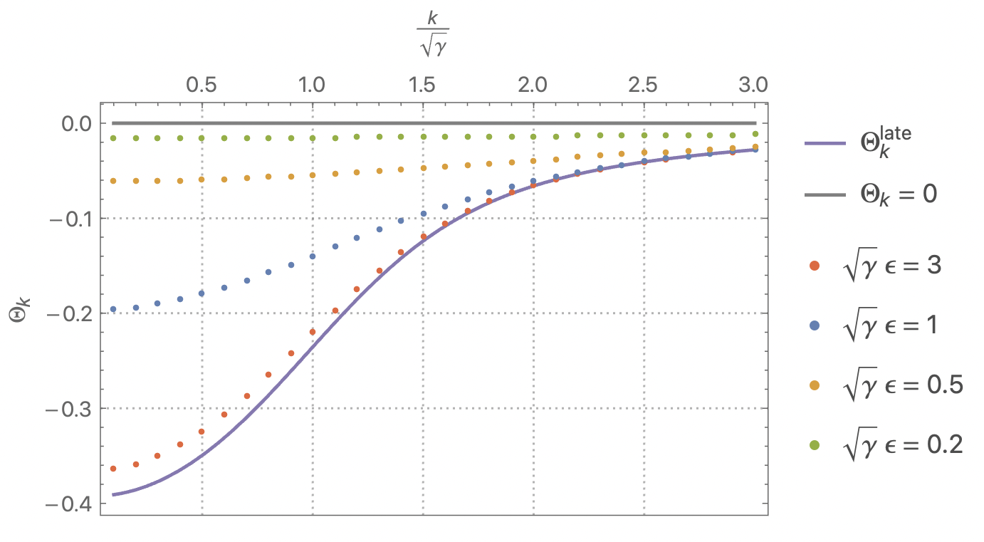
Figure 1: We represent $\Theta_{k}$ obtained with the states of low energy prescription for different values of $\epsilon$, $\sqrt{\gamma}\epsilon=3$ (red dots) and $\sqrt{\gamma}\epsilon=1$ (blue dots), $\sqrt{\gamma}\epsilon=0.5$ (orange dots) and $\sqrt{\gamma}\epsilon=0.2$ (green dots). We also represent the two limiting cases $\Theta_{k}=0$ (grey line) and $\Theta_{k}=\Theta_{k}^{late}$ (purple line).

In the next section we will illustrate how the above construction can be applied to a cosmological particle creation process of special relevance. It involves the production of heavy right-handed neutrinos by the radiation-dominated universe. To motivate the selection of this spin-$\frac{1}{2}$ field as a natural candidate for dark matter we will argue on the basis of conformal symmetry and anomaly cancellation.

6 Quantum stress-energy tensor and conformal symmetry

The (renormalized) vacuum expectation values of the stress-energy tensor in a FLRW spacetime can be expressed in the form [11, 30]

$$\langle T_{\mu\nu}\rangle=\langle T_{\mu\nu}\rangle_{0}+t_{\mu\nu}\ .$$ (62)

The tensor $\langle T_{\mu\nu}\rangle_{0}$ is traceless and it vanishes for conformal fields in the conformal vacuum. $t_{\mu\nu}$ is a geometric tensor accounting for the trace/conformal anomaly. It can be univocally derived from the trace anomaly and expressed as a linear combination of the geometric tensors ${}^{(3)}H_{\mu\nu}=\frac{1}{12}R^{2}g_{\mu\nu}-R^{\rho\sigma}R_{\rho\mu\sigma\nu}$ and ${}^{(2)}H_{\mu\nu}$. [In FLRW spacetimes ${}^{(1)}H_{\mu\nu}$ is proportional to ${}^{(2)}H_{\mu\nu}$ and ${}^{(3)}H_{\mu\nu}$ is a conserved tensor [20]].

As we approach back to the Big Bang, the stress-energy tensor is fully dominated by the conformal anomaly contribution $t_{\mu\nu}$. However, while the metric tensor

$$ds^{2}=a^{2}(\tau)(d\tau^{2}-d\vec{x}^{2})\ ,$$ (63)

is conformally regular as $\tau\to 0$, the conformally reescaled stress-energy tensor, in particular $a^{2}(\tau)t_{\mu\nu}$, is not longer regular at $\tau=0$. This is in tension with the basic idea behind the Weyl curvature hypothesis.

To solve the conflict one should require an exact cancellation of the conformal anomaly in the Standard Model. In a first approximation, we can ignore interactions and consider the free field content of the Standard Model living in a curved spacetime. The general expression for the conformal anomaly is given by

$$\langle T^{\mu}_{\mu}\rangle\equiv t^{\mu}_{\mu}=cC^{2}-aE\ ,$$ (64)

where $C^{2}$ is the square of the Weyl tensor and $E$ is the Euler density. We have omitted the contribution proportional to $\Box R$ since it is intrinsically ambiguous [10]. We are allowing geometries beyond exact FLRW, so $C^{2}$ does not need to be exactly zero. The relevant point here is that the coefficients $a$ and $c$, which depend on the spin of the field [20],

$$a = \frac{1}{360(4\pi)^{2}}[n_{0}+\frac{11}{2}n_{1/2}+62n_{1}]\ >0$$

$$c = \frac{1}{120(4\pi)^{2}}[n_{0}+3n_{1/2}+12n_{1}]\ >0\ ,$$ (65)

cannot cancel out. All conventional fields in the Standard Model contribute with the same sign. [$n_{0}\equiv$ number of scalar fields; $n_{1/2}\equiv$ number of spin-$1/2$ Weyl fields; $n_{1}\equiv$ number of spin-$1$ fields] For a recent discussion on the contribution of Weyl fermions see [31].

The cancellation of the conformal anomaly requires the introduction of a special scalar field $\phi^{\prime}$. Its action is expressed in terms of the unique conformally-invariant fourth order operator

$$S=\frac{1}{2}\int d^{4}x\sqrt{-g}\phi^{\prime}\triangle_{4}\ \phi^{\prime}\ ,$$ (66)

where $\triangle_{4}$ is given by [32, 33] (for other spin fields, see [34, 35])

$$\triangle_{4}=\Box^{2}+2R^{\mu\nu}\nabla_{\mu}\nabla_{\nu}-\frac{2}{3}R\Box+\frac{1}{3}(\nabla^{\mu}R)\nabla_{\mu}\ .$$ (67)

The contribution of this dimensionless scalar field $\phi^{\prime}$ to the conformal anomaly is given by [36]

$$a=-\frac{28}{360(4\pi)^{2}}\ \ \ \ \ \ c=-\frac{8}{120(4\pi)^{2}}\ .$$ (68)

The conformal anomaly is exactly cancelled for [37, 38]

$$n_{1/2}=4n_{1}=48\ ,\ \ \ \ \ \ \ \ \ n^{\prime}_{0}=3n_{1}=36\ ,\ \ \ \ \ \ n_{0}=0\,.$$

This corresponds to the current Standard Model, with exactly three generations, but with the following important caveats: i) one must include right-handed neutrinos, ii) the Higgs should be excluded as a fundamental field (it should emerge as a composite field), iii) one should also include $36$ scalar fields $\phi^{\prime}$. These special fields are very peculiar because they do not have particle excitations. They only contribute to the vacuum state [39].

6.1 Dark matter candidate for a time reversal and conformally invariant Big Bang

In the above context there is a natural candidate for dark matter. A heavy right-handed majorana neutrino $\nu^{R}$, decoupled from all of the other particles in the Standard Model. It can be only produced gravitationally [9]. Different initial phases produce then different cold dark matter spectra (48).

It is interesting to remember that for the Hadamard state of low energy centered at the Big Bang, we can consider a very small window function $\epsilon\to 0$. As it was shown in Fig. 1, for $\epsilon\to 0$ the SLE tends to $\Theta_{k}=0$ in the infrared regime. This can also be seen for the approximated SLE if we expand the analytical expression for a very small window function, $\Theta^{SLE}_{k}|_{\epsilon\to 0}\sim 0+O(\epsilon^{2})$. We want to remark this fact because the number density of created particle receives its major contribution from the infrared regime. Therefore, almost the same number density of created particles is obtained by using $\Theta_{k}=0$ or by using the state of low energy centered at the Big Bang with a very small window function. In Figure 2 we compare the prediction for $\Theta_{k}=\Theta_{k}^{late}$ and $\Theta_{k}=0$. In the following, we will compute the number density of created particles as a function of the state $\Theta_{k}$, and with this, we will obtain the resulting mass of the dark matter right handed neutrino for the states $\Theta_{k}=\Theta_{k}^{late}$ and $\Theta_{k}=0$.

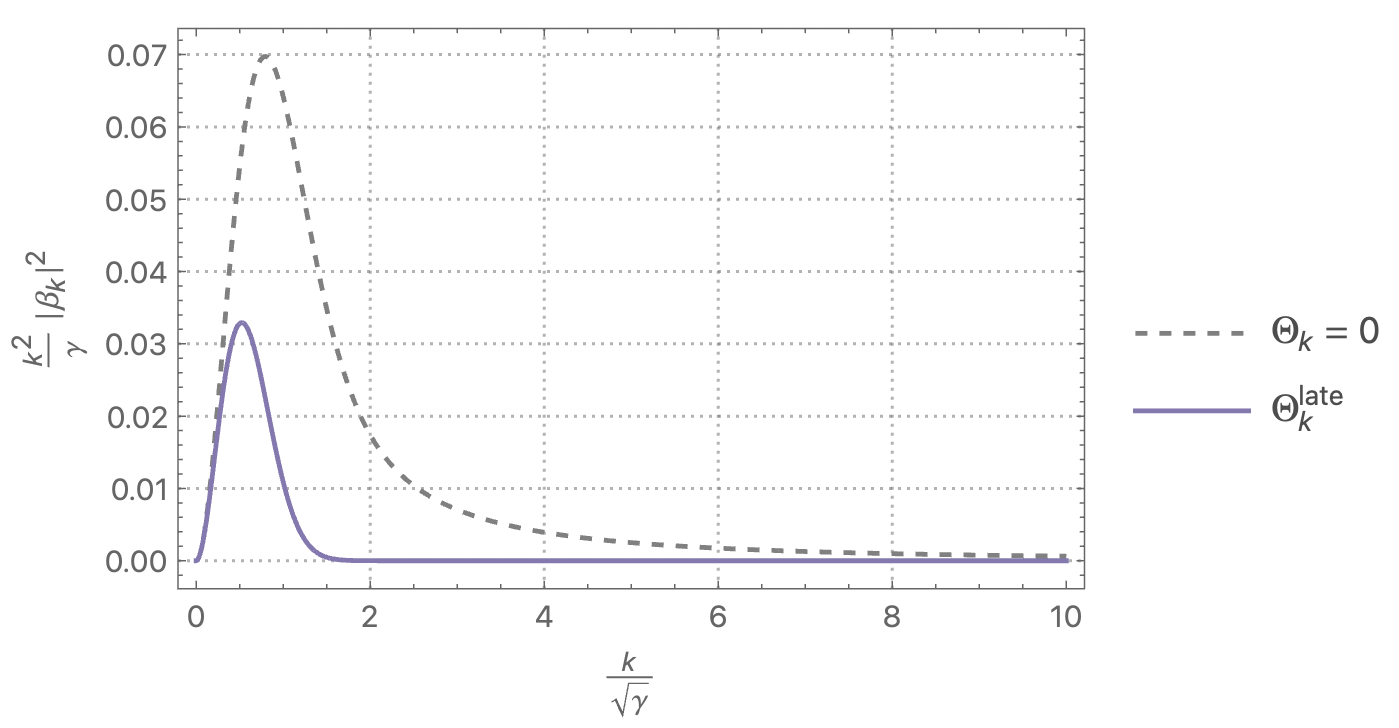
Figure 2: Comparison of the predicted spectra (cold dark matter) for two different vacua, namely $\Theta_{k}^{late}$ and $\Theta_{k}=0$.

From the results of Section 5, the comoving number density of created right-handed neutrinos is given by

$$n_{dm}=\sum_{h}\int\frac{d^{3}k}{(2\pi)^{3}}|\beta_{k}|^{2}=(\gamma/\pi)^{3/2}I_{\Theta_{k}}\,.$$ (69)

$I_{\Theta_{k}}$ is the dimensionless integral given by

$$I_{\Theta_{k}}=\frac{4}{\sqrt{\pi}}\int_{0}^{\infty}d\kappa\sqrt{\kappa}|\beta_{k}|^{2}\,,$$ (70)

where $|\beta_{\kappa}|^{2}$ is given by the right hand side of (48). Furthermore, the physical energy density of the cold dark matter created is diluted in cosmological time $t$ according to

$$\rho_{dm}(t)=\frac{M_{\Theta_{k}}}{a^{3}}\sum_{h}\int\frac{d^{3}k}{(2\pi)^{3}}|\beta_{k}|^{2}=\frac{M_{\Theta_{k}}}{a^{3}}(\gamma/\pi)^{3/2}I_{\Theta_{k}}=\frac{M_{\Theta_{k}}}{(2\pi)^{3/2}}\left(\frac{M_{\Theta_{k}}}{t}\right)^{3/2}I_{\Theta_{k}}\,.$$ (71)

To obtain a prediction for $M_{dm}$ from the observed value of the energy density of dark matter we follows now the argument in [8]. For $\Theta_{k}^{late}$ used in [8] one gets $I_{\Theta_{k}^{late}}=0.01276$ and then $M_{\Theta_{k}^{late}}=4.8\times 10^{8}GeV$. If we now change the quantum state, the prediction for the mass changes accordingly

$$M_{\Theta_{k}^{late}}^{5/2}I_{\Theta_{k}^{late}}=M_{\Theta_{k}}^{5/2}I_{\Theta_{k}}\,.$$ (72)

For $\Theta_{k}=0$ we have $I_{\Theta_{k}=0}=0.06305$ and hence $M_{\Theta_{k}=0}=2.6\times 10^{8}GeV$.

7 Conclusions

A straightforward realization of the Weyl curvature hypothesis has been considered by assuming an early universe dominated by radiation and extending the expansion factor analytically to negative values of conformal time. In this context, the problem of selecting a preferred vacuum state is discussed by enforcing the emergent symmetry of the metric under the transformation $\tau\to-\tau$. One possible vacuum choice, as suggested in [9], is the $T$-invariant linear combination $|0_{T}\rangle\propto|0_{+}\rangle+|0_{-}\rangle$, where $|0_{+}\rangle$ and $|0_{-}\rangle$ are the adiabatic vacua at $\tau\to\pm\infty$, respectively.

An alternative option is to define a vacuum state around $\tau\sim 0$. This option is more involved and can be formulated using the states of low energy prescription. In this framework, the vacuum state is defined as the state that minimizes the energy density averaged over a temporal window function $f^{2}$. It is important to emphasize that this approach yields vacuum states that satisfy the Hadamard condition, which is crucial to obtain finite quantities for vacuum expectation values of the stress-energy tensor, and its fluctuations, after renormalization.

The states obtained with this method allow some interesting physical predictions. First, primordial gravitational waves can be produced even though the initial state of the universe is well-described by a radiation-dominated era. Second, the mass of the natural candidate for dark matter in this scenario, namely, a heavy right-handed Majorana neutrino $\nu^{R}$ is of order $10^{8}GeV$. The specific prediction for the mass slightly depends on the selection of the vacuum state.

Appendix A Details on the large momentum expansion of the scalar field modes

This short appendix gives supplementary material to the analysis given in [25] for more general hyperbolic phases $\theta_{k}$. For an arbitrary value of $\theta_{k}$ we cannot ensure that the stress-energy tensor is renormalizable with the standard subtractions. We have to analyze the problem with the technique displayed in [25]. In short, we have to look at the large $k$ expansion of the modes $\varphi_{k}$

$$|\varphi_{k}(\tau)|^{2} \sim \cosh(2\theta_{k})\left(\frac{1}{k}-\frac{\gamma^{2}\tau^{2}}{2k^{3}}+\frac{3\gamma^{4}\tau^{4}}{8k^{5}}+\frac{\gamma^{2}}{4k^{5}}-\frac{\gamma^{2}\cos(2k\tau)}{4k^{5}}+\mathcal{O}\left(\frac{1}{k^{6}}\right)\right)$$

$$+\sinh(2\theta_{k})\left(-\frac{\gamma^{2}}{4k^{5}}+\frac{\cos(2k\tau)}{k}-\frac{\gamma^{2}\tau^{3}\sin(2k\tau)}{3k^{2}}\right.$$

$$\left.-\frac{\gamma^{4}\tau^{6}\cos(2k\tau)}{18k^{3}}-\frac{\gamma^{2}\tau^{2}\cos(2k\tau)}{2k^{3}}+\mathcal{O}\left(\frac{\sin(2k\tau)}{k^{4}}\right)\right)\ .$$

To get a finite $\langle 0|T_{\mu\nu}|0\rangle_{ren}$ the non-oscillatory terms must coincide with the adiabatic expansion obtained from (18) up to and including the order $k^{-5}$. These are exactly the non-oscillatory terms inside the parenthesis multiplying to $\cosh(2\theta_{k})$. Therefore, the factor $\cosh(2\theta_{k})$ can only add corrections of order $\sim k^{-5}$. Taking into account the Taylor expansion of the hyperbolic cosine, we can easily conclude that the leading order in the ultraviolet expansion of $\theta_{k}$ must be at least of order $k^{-5/2}$. On the other hand, the leading oscillatory term must also decay, at least, as $k^{-n},n>4$. This ensures a well behaved integral for the energy density and pressure in the ultraviolet regime, (see [25]). Therefore the factor $\sinh(2\theta_{k})$ can only add corrections of order $k^{-n},n>3$. Using the expansion of the hyperbolic sine, we see that the leading order in the ultraviolet expansion of $\theta_{k}$ must be at least of order $k^{-n},n>3$. Therefore the asymptotic form of $\theta_{k}$ should be $\theta_{k}\sim\mathcal{O}(k^{-n}),\,n>3$.

Appendix B Details on the large momentum expansion of the spin-$1/2$ field modes

In this brief appendix, we give the large $k$ expansion of the integrand of the formal vacuum expectation value of the energy density $\rho_{k}(\tau)$, defined as

$$\langle T_{00}\rangle=\frac{1}{(2\pi)^{2}a^{3}}\int_{0}^{\infty}k^{2}dk\,\rho_{k}(\tau)\ ,$$ (74)

for the CPT-invariant vacuum states characterized by $\Theta_{k}$ (see Ref. [30] for details regarding $\langle T_{\mu\nu}\rangle_{ren}$ for Dirac fields in spatially flat FLRW backgrounds and [13] for the explicit form of the modes in the CPT-invariant radiation-dominated universe). Using the techniques displayed in [25] we find

$$m^{-1}\rho_{k}(\tau) \sim \cos(2\Theta_{k})\Bigg{(}-\frac{2k}{\gamma\tau}-\frac{\gamma\tau}{k}+\frac{\gamma}{2k^{3}\tau}+\frac{\gamma^{3}\tau^{3}}{4k^{3}}-\frac{\gamma\cos(2k\tau)}{2k^{3}\tau}+\mathcal{O}\left(\frac{\sin(2k\tau)}{k^{4}}\right)\Bigg{)}$$

$$+\sin(2\Theta_{k})\Bigg{(}+\frac{1}{k\tau}+\frac{\gamma^{2}\tau}{2k^{3}}-\frac{\cos(2k\tau)}{k\tau}+\frac{\gamma^{2}\tau^{2}\sin(2k\tau)}{3k^{2}}+\mathcal{O}\left(\frac{\cos(2\kappa\tau)}{k^{3}}\right)\Bigg{)}\,.$$

This expression has to be compared with the large $k$ expansion of the adiabatic expansion of the energy density, namely

$$m^{-1}\rho_{k}(\tau)^{ad}\sim-\frac{2k}{\gamma\tau}-\frac{\gamma\tau}{k}+\frac{\gamma}{4k^{3}\tau}-\frac{\gamma^{3}\tau^{3}}{4k^{3}}+\mathcal{O}\left(\frac{1}{k^{5}}\right)\,.$$ (76)

In this case, and since we are directly looking at the energy density, we need to find coincidence with the adiabatic expansion up to and including order $\mathcal{O}(k^{-3})$. We directly see that, for $\Theta_{k}=0$, there is one term in (B), $\gamma/(2k^{3}\tau)$, that does not coincide with the adiabatic expansion, generating a logarithmic divergence after renormalization. On the contrary, for $\Theta_{k}\sim-\frac{\gamma}{4k^{2}}$, and using the large $k$ expansion of the trigonometric functions, we see that the part proportional to $\sin(2\Theta_{k})$ contributes to the large $k$ expansion in such a way that we recover the adiabatic expansion (76), making the energy density UV regular. Furthermore, in this case we find also cancellations for the oscillatory terms. We have also performed a similar analysis with the two-point function and the pressure, finding analogous results. We have found that, to ensure the convergence of these three quantities, the trigonometric phase should behave, at large $k$, as $\Theta_{k}\sim-\frac{\gamma}{4k^{2}}+\mathcal{O}(k^{-n}),\ n>2$.

References

References

- [1] Penrose R 1979 General Relativity: An Einstein Centenary Survey, edited by Hawking S W and Israel W (Cambridge, UK: Cambridge University Press) pp 581–638
- [2] Penrose R 1969 Riv. Nuovo Cim. 1 252–276
- [3] Newman R P A C 1993 Proc. Roy. Soc. Lond. A 443 493–515
- [4] Audretsch J and Schaefer G 1978 J. Phys. A 11 1583–1602
- [5] Parker L 1966 The creation of particles in an expanding universe Ph.D. thesis Harvard University
- [6] Parker L 1968 Phys. Rev. Lett. 21 562–564
- [7] Parker L 1969 Phys. Rev. 183 1057–1068
- [8] Boyle L, Finn K and Turok N 2022 Annals Phys. 438 168767 (Preprint 1803.08930)
- [9] Boyle L, Finn K and Turok N 2018 Phys. Rev. Lett. 121 251301 (Preprint 1803.08928)
- [10] Wald R M 1995 Quantum Field Theory in Curved Space-Time and Black Hole Thermodynamics Chicago Lectures in Physics (Chicago, IL: University of Chicago Press) ISBN 978-0-226-87027-4
- [11] Parker L E and Toms D 2009 Quantum Field Theory in Curved Spacetime: Quantized Field and Gravity Cambridge Monographs on Mathematical Physics (Cambridge University Press) ISBN 978-0-521-87787-9
- [12] Olbermann H 2007 Class. Quant. Grav. 24 5011–5030 (Preprint 0704.2986)
- [13] Nadal-Gisbert S, Navarro-Salas J and Pla S 2023 Low Energy States and CPT invariance at the Big Bang [to appear in PRD] (Preprint 2302.08812)
- [14] Abramowitz M and Stegun I A 1964 Handbook of Mathematical Functions with Formulas, Graphs, and Mathematical Tables (Dover Publications)
- [15] Parker L and Fulling S A 1974 Phys. Rev. D 9 341–354
- [16] Fulling S A and Parker L 1974 Annals Phys. 87 176–204
- [17] Fulling S A, Parker L and Hu B L 1974 Phys. Rev. D 10 3905–3924
- [18] Anderson P R and Parker L 1987 Phys. Rev. D 36 2963
- [19] Beltrán-Palau P, del Río A, Nadal-Gisbert S and Navarro-Salas J 2021 Phys. Rev. D 103 105002 (Preprint 2103.17218)
- [20] Birrell N D and Davies P C W 1984 Quantum Fields in Curved Space Cambridge Monographs on Mathematical Physics (Cambridge, UK: Cambridge Univ. Press) ISBN 978-0-521-27858-4
- [21] Pirk K T 1993 Phys. Rev. D 48 3779–3783 (Preprint gr-qc/9211003)
- [22] Brunetti R and Fredenhagen K 2000 Commun. Math. Phys. 208 623–661 (Preprint math-ph/9903028)
- [23] Hollands S and Wald R M 2001 Commun. Math. Phys. 223 289–326 (Preprint gr-qc/0103074)
- [24] Hollands S and Wald R M 2002 Commun. Math. Phys. 231 309–345 (Preprint gr-qc/0111108)
- [25] Beltrán-Palau P, Nadal-Gisbert S, Navarro-Salas J and Pla S 2022 Renormalization and a non-adiabatic vacuum choice in a radiation-dominated universe (Preprint 2204.05404)
- [26] Banerjee R and Niedermaier M 2020 J. Math. Phys. 61 103511 (Preprint 2006.08685)
- [27] Ford L H and Parker L 1977 Phys. Rev. D 16 1601–1608
- [28] Landete A, Navarro-Salas J and Torrenti F 2013 Phys. Rev. D 88 061501 (Preprint 1305.7374)
- [29] Landete A, Navarro-Salas J and Torrenti F 2014 Phys. Rev. D 89 044030 (Preprint 1311.4958)
- [30] del Rio A, Navarro-Salas J and Torrenti F 2014 Phys. Rev. D 90 084017 (Preprint 1407.5058)
- [31] Abdallah S, Franchino-Viñas S A and Fröb M B 2021 JHEP 03 271 (Preprint 2101.11382)
- [32] Paneitz M 1983 Typeset by the Editors for the Proceedings of the Midwest Geometry Conference 2007 (Preprint 0803.4331)
- [33] Reigert R J 1984 Phys. Lett. B 134 56–60
- [34] de Berredo-Peixoto G and Shapiro I L 2001 Phys. Lett. B 514 377–384 (Preprint hep-th/0101158)
- [35] Stergiou A, Vacca G P and Zanusso O 2022 JHEP 06 104 (Preprint 2202.04701)
- [36] Gusynin V P 1989 Phys. Lett. B 225 233–239
- [37] Boyle L and Turok N 2021 (Preprint 2110.06258)
- [38] Miller J, Volovik G E and Zubkov M A 2022 Phys. Rev. D 106 015021 (Preprint 2202.05726)
- [39] Bogolubov N N Logunov A A Oksak A I and Todorov I T 1990 General Principles of Quantum Field Theory (Dordrecht: Academic Publishers)