A Switching Thrust Tracking Controller for Load Constrained Wind Turbines

Abstract

Wind turbines are prone to structural degradation, particularly in offshore locations. Based on the structural health condition of the tower, power de-rating strategies can be used to reduce structural loads at the cost of power losses. This paper introduces a novel closed-loop switching control architecture to constrain the thrust in individual turbines. By taking inspiration from developments in the field of reference governors, an existing demanded power tracking controller is extended by a thrust tracking controller. The latter is activated only when a user-defined constraint on fore-aft thrust force is exceeded, which can be set based on the actual damage status of the turbine. Having a down-regulation with monotonic aerodynamic load response, a simple linear thrust tracking controller is proposed. Such a scheme can reduce aerodynamic loads while incurring acceptable losses on power production which, in a wind farm setting, can be compensated for by other turbines. Large eddy simulations demonstrate the performance of the proposed scheme on satisfying thrust constraints.

I INTRODUCTION

To make wind energy competitive in the transition from fossil fuel-based to renewable energy sources, it is essential to reduce the Levelized Cost of Energy (LCoE). This performance indicator takes into account the costs of construction, maintenance and the energy generated by the power plant over its entire lifetime [1].

Structural degradation reduces the lifetime of turbine components as an inevitable result of alternating stresses and environmental conditions, thereby increasing the cost of maintenance. Periodic structural loading is being considered as the main cause for component failures [2, 3]. Additionally, structural degradation is accelerated by the offshore environment, including wave action and corrosion[4].

A way to reduce the damage propagation and increase reliability is by derating the turbine appropriately to reduce structural stresses. Health monitoring systems can be used to detect and to estimate high level corrosion, mechanical flaws and cracks [5, 6]. Although this results in sub-optimal power generation for individual turbines, the turbines’ structural reliability is improved, where fatigue damage is alleviated and lifetime extended [7]. As a result, the turbine is able to continue operating as opposed to shutting down, until maintenance is fully performed.

When the goal of the wind farm controller is to track a power reference, and enough power is available in the wind, the power contributions from individual turbines can be redistributed among the turbines in the farm. That is, reducing the demanded power for a set of turbines, is compensated for by increasing the power reference for the other turbines. This can be accomplished by simple compensation control loops as described in [8]. For instance, power losses due to waked conditions are compensated when turbines are not able to meet their individual power reference in [9].

At an individual turbine level, the down-regulation of power can be achieved by either operating the turbine at higher rotor speeds (HRS) or lower rotor speeds (LRS), with respect to the rotor speed from conventional controllers.

HRS approaches are beneficial for power tracking because there is more kinetic energy associated with the higher rotor speed, allowing fast recovery when demanded power increases. As an HRS approach, the Max-$\Omega$ strategy [10] maximizes the rotor speed. However, the HRS approaches present limitations for our design. The aerodynamic loads do not reduce significantly when the power demand decreases and might even increase [11]. As a result of the latter, the thrust response might not be monotone to power setpoint changes. Non-monotone behaviors do not only appear in the thrust and power relation, but they can also appear in the demanded power and generated power relation [12].

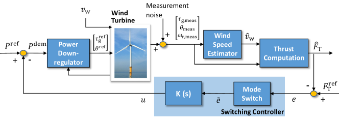
Figure 1: Block diagram of the proposed switching control architecture for constraining the turbine thrust forces. The novel switching controller is highlighted in light blue.

LRS approaches present lower aerodynamic loads and, consequently, lower structural loads on the blades and tower. In constrast with HRS approaches, the turbine response presents a monotone behavior from power demand to thrust. As an LRS approach, the Const-$\Omega$ [13] keeps the rotor speed constant avoiding high rotor speeds, but can reach extreme tip-speed ratio values and undesirable operation regions as wind speed changes. Furthermore, there exists the so-called min-C_T method based on steady state power coefficient (C_P) and thrust coefficient (C_T) look-up tables [13, 14]. C_P and C_T represent the wind turbine power and thrust conversion efficiencies, respectively. The method ideally leads to the smallest thrust compared to all the down-regulation strategies and demonstrates benefits for waked wind farms, which allows more available power to down-stream turbines [15, 16]. However, its operation in low tip-speed ratios is close to stall conditions, where the predominant flow stability along the blades can be lost, affecting the controlled turbine response. This latter drawback is overcome in [17] and [18] with the so-called “Active Power Control (APC) pitch” and KNU2, respectively. This approach pitches the blades to follow a reference generator speed, based on the function built from the conventional generator torque law [19, 20]. Although the power tracking response is slightly worse in the LRS approaches [17], [18], they are suitable for wind farm power tracking purposes on large farms. For instance, down-regulation providing power reserves were explored in [21].

This paper proposes a switching control architecture for wind turbines that must satisfy a user-defined constraint on the fore-aft thrust forces. This architecture allows to track a demanded power profile when the thrust forces are lower than a given maximum allowed value. When such a value is reached, the proposed controller switches from tracking the demanded power to tracking the maximum allowed thrust force, thus satisfying the constraint on the turbine maximum loading. In particular, the following contributions are presented:

1. The extension of an existing power tracking controller via a switching thrust tracking feedback law that modifies the former’s reference, by taking inspiration from the reference governor literature [22];

2. The introduction of an integral switching law for the thrust tracking controller in order to avoid chattering when the estimate thrust force lies on the constraint boundary;

3. A large eddy simulation (LES) study showing the effectiveness of the proposed scheme for both laminar and turbulent wind speed profiles.

The simulation study shows how the relative reduction in the thrust force results in a generated power reduction experienced by a given turbine. This allows to satisfy constraints on structural load, which can depend for instance on the current turbine state of structural health. Furthermore, the present paper will pave the way for the design of a wind farm power allocation control scheme, where healthy turbines can be assigned a larger demanded power to compensate for reductions in turbines that operate at their maximum allowed structural load.

The structure of this paper is as follows. First, the switching thrust tracking controller design is outlined in Section II. Next, the down-regulation method is discussed in Section II-D. Section III presents simulation results of the proposed thrust tracking controller. Finally, the paper is concluded in Section IV.

II Switching Control Architecture

This section presents the proposed switching control architecture for load constraining. First an overview of the architecture will be given. Then, the individual constituting blocks, namely the thrust estimator, the thrust tracking controller, the switching law, and the demanded power down regulator will be described.

II-A Overview of the architecture

The overall switching control architecture is presented in Figure 1, where we assume that external references $P^{\textrm{ref}}\in\mathbb{R}^{+}$ and $F_{T}^{\textrm{ref}}\in\mathbb{R}^{+}$ are provided for, respectively, the power to be generated by the given wind turbine and the maximum allowed fore-aft thrust forces. Starting from left, we can identify the following functional blocks

1. The power down-regulator $\mathcal{D}$, which can track a demanded power $P^{\textrm{dem}}\leq P^{\textrm{av}}$, where $P^{\textrm{av}}$ is the available aerodynamic power. $\mathcal{D}$ provides to the turbine a reference $\theta^{\textrm{ref}}$ and $\tau_{\textrm{g}}^{\textrm{ref}}$ for, respectively, the collective blade pitch and the generator torque (see Section II-D).

2. The wind turbine, which accepts as inputs the references $\theta^{\textrm{ref}}$ and $\tau_{\textrm{g}}^{\textrm{ref}}$ and provides the output measurements $\omega_{\textrm{r},\textrm{meas}}$, $\tau_{\textrm{g, meas}}$ and $\theta_{\textrm{meas}}$ representing the rotor speed, generator torque and the collective blade pitch angle, respectively.

3. The wind speed estimator, which uses the measurements $\omega_{\textrm{r},\textrm{meas}}$ and $\theta_{\textrm{meas}}$ to compute an estimate $\hat{v}_{\textrm{w}}$ of the rotor effective wind speed $v_{\textrm{w}}$. As in the present work we do not assume to have a reliable wind speed measurement, so the Immersion and Invariance (I&I) wind speed estimator of [23] will be used.

4. The thrust computation block, which uses the wind speed estimate $\hat{v}_{\textrm{w}}$, $\omega_{\textrm{r},\textrm{meas}}$ and $\theta_{\textrm{meas}}$ to compute an estimate of the fore-aft thrust force $\hat{F}_{\textrm{T}}$.

5. The mode switch block, which together with the transfer function $K(s)$ constitutes the novel switching controller proposed in the present paper for tracking the thrust force. The output of $K(s)$ is the signal $u$, which is subtracted from the external reference $P^{\textrm{ref}}$ to obtain the demanded power $P^{\textrm{dem}}=P^{\textrm{ref}}-u$.

In order to derive the proposed switching controller, we will introduce the following

Assumption 1

The down-regulation controller and wind speed estimator are asymptotically stable, as in [17, 18, 23].

Assumption 2

The dynamics from the demanded power to thrust force are represented by a first-order linear model as

$$\frac{F_{\mathrm{T}}(s)}{P^{\mathrm{dem}}(s)}=\frac{A}{s+B}\overset{\operatorname{def}}{=}G(s).$$ (1)

Remark 1

As Assumption 1 holds, in steady conditions both generated power and thrust force will converge to a constant value. Short term transient behaviors in the turbine operation are not the focus of our controller. This justifies the use of Assumption 2 for representing the dominant behavior.

We are now ready to introduce the control problem addressed by the present paper:

Problem 1

Design a feedback control law that extends, rather than replacing, the existing demanded power controller $\mathcal{D}$ such that:

1. the fore-aft thrust force $F_{\textrm{T}}$ does not exceed a user defined upper bound $\bar{F}_{\textrm{T}}$;

2. the tracking performance of the desired power reference $P^{\textrm{ref}}$ is unaltered whenever $F_{\textrm{T}}\leq\bar{F}_{\textrm{T}}$.

The next subsection introduces the novel switching controller developed in this paper.

II-B Switching Controller Design

This section describes the design of the Mode Switch and the transfer function $K(s)$ introduced in previous subsection, towards solving the control problem posed in Problem 1.

The first observation is that, in order to satisfy point 2 in Problem 1, it is sufficient that the signal $u$ becomes zero, and thus $P^{\textrm{dem}}=P^{\textrm{ref}}$. In order to do this, the Mode Switch will be designed such that the lower feedback loop in Figure 1 will be open whenever the constraint on the thrust force is not exceeded. In particular, the switching will be defined by introducing the following signal

$$\tilde{e}=\begin{cases}e,&\text{if }e<0\ \text{ or }e_{\mathrm{I}}<0\\ 0,&\text{otherwise}\end{cases}$$ (2)

where $e=F_{\textrm{T}}^{\mathrm{ref}}-\hat{F}_{\mathrm{T}}$ and $e_{\mathrm{I}}=\int_{0}^{t}{e(\tau)}\textrm{d}\tau$ represent, the difference between the estimated thrust force and its reference, herein set as equal to the upper bound, i.e. $F_{\textrm{T}}^{\mathrm{ref}}$ = $\bar{F}_{\textrm{T}}$, and the time integral of that, respectively. The rationale for this definition with the inclusion of the integral term is to avoid chattering when the thrust force is close to its reference, as is done for instance in the literature on Integral Sliding Mode control [24].

When the mode switch is active, that is when $\tilde{e}\neq 0$, the lower feedback loop involving the transfer function $K(s)$ is closed. The design of $K(s)$, outlined in the subsequent part, will thus determine the fulfillment of requirement 1 in Problem 1.

The approach is to design $K(s)$ such that $\hat{F}_{\mathrm{T}}$ will track its reference $F_{\textrm{T}}^{\mathrm{ref}}$. From this point of view, notice that variations of the power reference and wind speed also contribute to the thrust response. As such, $P^{\mathrm{ref}}$ and $v_{\mathrm{w}}$ are considered disturbances acting into the system. This said, the thrust response can be written in the Laplace domain as

$$F_{\mathrm{T}}(s)=-G(s)u(s)+G_{\mathrm{d,\,1}}(s)P^{\mathrm{ref}}(s)+G_{\mathrm{d,\,2}}(s)v_{\mathrm{w}}(s),$$ (3)

$$\mathrm{where}\,\,\,\,\,\ u(s)=-K(s)\tilde{e}(s)=-K(s)\left(F_{\mathrm{T}}^{\mathrm{ref}}(s)-F_{\mathrm{T}}(s)-n(s)\right).$$ (4)

$G(s)$ represents the transfer function of the join power down-regulator and wind turbine from the considered demanded power $P^{\mathrm{dem}}$ input and the thrust $F_{\mathrm{T}}$ output. $G_{\mathrm{d,\,1}}(s)=G(s)$ from $P^{\mathrm{ref}}$ to $F_{\mathrm{T}}$ and $G_{\mathrm{d,\,2}}(s)$ from $v_{\mathrm{w}}$ to $F_{\mathrm{T}}$ are the transfer functions from the considered disturbances on the down-regulated turbine. Furthermore, $n(s)=F_{\mathrm{T}}(s)-\hat{F}_{\mathrm{T}}(s)$ represents the estimation error between the true thrust and the estimated one (cfr. Section II-C).

Substituting Eq. (4) into Eq. (3), and reorganizing the terms we have the closed-loop response as

$$\begin{array}[]{cc}F_{\mathrm{T}}(s)&=\dfrac{K(s)G(s)}{1+K(s)G(s)}F_{\mathrm{T}}^{\mathrm{ref}}(s)+\dfrac{G_{\mathrm{d,\,1}}(s)}{1+K(s)G(s)}P^{\mathrm{ref}}(s)\\ &\\ &+\dfrac{G_{\mathrm{d,\,2}}(s)}{1+K(s)G(s)}v_{\mathrm{w}}(s)-\dfrac{K(s)G(s)}{1+K(s)G(s)}n(s).\end{array}$$ (5)

The controller $K(s)$ should be designed to stabilize the poles of the closed-loop system, i.e. the roots of $1+K(s)G(s)=0$, and to guarantee steady-state convergence from changes in the reference, disturbances and estimation error. A PI controller is therefore chosen in this paper as an effective way to track the reference, to reject the disturbances and to attenuate the estimation error

$$K(s)=K_{\mathrm{P}}+\frac{K_{\mathrm{I}}}{s}.$$ (6)

The closed-loop characteristic equation is then equal to

$$s^{2}+(B+K_{\mathrm{P}}A)s+K_{\mathrm{I}}A=s^{2}+2\zeta\omega_{\mathrm{n}}s+\omega_{\mathrm{n}}^{2}=0.$$ (7)

Proposition 1

The steady-state thrust tracking error is bounded for steps in reference, disturbances and estimation error.

Using Eq. 5, we can derive the thrust tracking error function

$$\begin{array}[]{cl}E(s)&=F_{\mathrm{T}}(s)-F_{\mathrm{T}}^{\mathrm{ref}}(s)\\ &=\underbrace{\left(T(s)-1\right)F_{\mathrm{T}}^{\mathrm{ref}}(s)}_{E_{1}(s)}+\underbrace{S(s)G_{\mathrm{d,\,1}}(s)P^{\mathrm{ref}}(s)}_{E_{2}(s)}\\ &\,\,\,\,+\underbrace{S(s)G_{\mathrm{d,\,2}}(s)v_{\mathrm{w}}(s)}_{E_{3}(s)}-\underbrace{T(s)n(s)}_{E_{4}(s)}\,,\end{array}$$ (8)

where $S(s)=1/(1+K(s)G(s))$ and $T(s)=K(s)G(s)/(1+K(s)G(s))$ are the sensitivity and complementary sensitivity functions, respectively.

By the final value theorem, the state steady errors due to steps on $F_{T}^{\mathrm{ref}}$, $P^{\mathrm{ref}}$, $v_{\mathrm{w}}$, and $n$ can be computed for the proposed controller as

$$\begin{array}[]{cl}e_{\mathrm{ss},i}&=\lim_{t\to\infty}e_{i}(t)\\ &=\lim_{s\to 0}sE_{i}(s),\end{array}$$ (9)

where $i=1,2,3,4$.

By Assumption 1, $G_{\mathrm{d,\,1}}(s)$ and $G_{\mathrm{d,\,2}}(s)$ are stable functions, as well as the estimation error $n$ is bounded. Therefore, the steady state error vector is $e_{\mathrm{ss}}=[0,\,0,\,0,\,-T(0)]$ for steps on $F_{T}^{\mathrm{ref}}$, $P^{\mathrm{ref}}$, $v_{\mathrm{w}}$, and $n$.

Remark 2

The controller can be calibrated with an offset in to the thrust reference to take into account $e_{\mathrm{ss,4}}$ if a constant bias in the thrust estimation exists. In addition, extra measurement devices can be used to improve the estimations and reduce the bias, such as the use of strain-gauges or accelerometers in the tower structure.

Remark 3

Deviations in the model from Assumption 2 can occur at different wind speeds given the non-linearity of the turbines, therefore it might degrade the designed controller performance. Nevertheless, as Assumption 1 and monotonicity from $\mathcal{D}$ still hold, the tracking is kept, as well as steps from disturbances rejected and from noise attenuated, even though model uncertainties exist.

II-C Thrust Computation

The estimated average fore-aft thrust force, representing the aerodynamic loads, is computed by

$$\hat{F}_{\mathrm{T}}=0.5\rho\pi R^{2}{\hat{v}_{\mathrm{w}}^{2}}C_{\mathrm{T}}\left(\frac{R\omega_{\textrm{r},\textrm{meas}}}{\hat{v}_{\mathrm{w}}},\theta_{\textrm{meas}}\right),$$ (10)

where $\hat{v}_{\mathrm{w}}$ is the estimated effective wind speed, $\rho$ the air density, $R$ the rotor radius and $C_{\mathrm{T}}$ the thrust coefficient computed with the measured rotor speed $\omega_{\textrm{r},\textrm{meas}}$ and collective blade pitch angle $\theta_{\textrm{meas}}$. In this work, the estimation of the effective wind speed is obtained from the I&I estimator [23] through measurements of rotor speed, generator torque and blade pitch angles.

II-D Power down-regulator

For the down-regulator $\mathcal{D}$ the APC pitch approach [17, 18] is adopted in this work, because of the following characteristics:

• A monotonic thrust reduction in response to monotonic demanded power reduction is achieved;

• Operation close to the min-$C_{T}$ method, see Fig. 2;

• Stability margin for the stall region [12].

The turbine is down-regulated using the blade pitch controller, which consists of a gain-scheduled PI control law

$$\begin{array}[]{cc}\theta=&\overline{K}_{\mathrm{P}}(\theta_{\mathrm{meas}})\left[\omega_{\mathrm{g,\,meas}}-\omega_{\mathrm{g}}^{\mathrm{ref}}(P^{\mathrm{dem}})\right]\\ &\,\,\,\,+\dfrac{\overline{K}_{\mathrm{I}}(\theta_{\mathrm{meas}})}{s}\left[\omega_{\mathrm{g,\,meas}}-\omega_{\mathrm{g}}^{\mathrm{ref}}(P^{\mathrm{dem}})\right],\end{array}$$ (11)

where $\omega_{\mathrm{g,\,meas}}$ and $\theta_{\mathrm{meas}}$ are the measured generator speed and the measured collective blade pitch angle, respectively. The reference generator speed as function of the demanded power $P^{\mathrm{dem}}$ is represented by $\omega_{\mathrm{g}}^{\mathrm{ref}}(P^{\mathrm{dem}})$. $\overline{K}_{\mathrm{P}}(\theta_{\mathrm{meas}})$ and $\overline{K}_{\mathrm{I}}(\theta_{\mathrm{meas}})$ are the gain-scheduled proportional and integral gains [25]. While the generator torque controller is applied to track the demanded power by multiplying it by the inverse of the measured generator speed as

$$\tau_{\mathrm{g}}=\frac{P^{\mathrm{dem}}}{\eta_{\mathrm{eff}}\omega_{\mathrm{g,\,meas}}}.$$ (12)

Both controllers are applied whenever the demanded power is lower than the rated power, and the measured generator speed is higher than the reference generator speed or the blade pitch angle is higher than a switch blade pitch angle. Otherwise, the turbine follows the conventional turbine controllers [25].

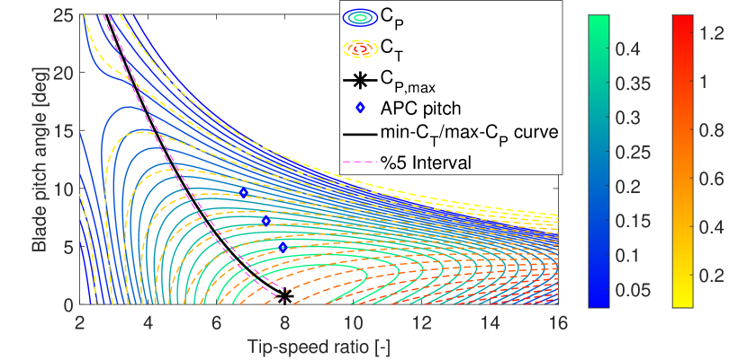
Figure 2: C_P and C_T of the operation points of “APC pitch” given a reduction in the demanded power (5, 4 and 3 MW) at 9 m/s wind speed and min-C_T/max-C_P curve for the DTU 10MW reference wind turbine.

III SIMULATIONS AND DISCUSSIONS

The proposed control architecture is evaluated in the high-fidelity simulation environment, Simulator for Wind Farm Applications (SOWFA), developed by the National Renewable Energy Laboratory [26]. SOWFA implements the actuator line method, embedded in a computational fluid dynamics flow, accounting for the Coriolis force and Buoyancy effects. Capturing turbine interactions, SOWFA was chosen aiming for future wind farm investigations. The DTU 10MW reference wind turbine is used in this work [27]. The control parameters of the controllers are based on the values provided with the NREL’s Reference OpenSource Controller (ROSCO) [25]. An overview of the parameters for the SOWFA simulations in this paper is shown in Table I.

TABLE I: SOWFA simulation parameters

Property	Value
Sub-grid-scale model	One-equation eddy viscosity
Domain size	3 km $\times$ 3 km $\times$ 1 km
Cell size outer regions	10 m $\times$ 10 m $\times$ 10 m
Cell size near rotor	2.5 m $\times$ 2.5 m $\times$ 2.5 m
Simulation timestep	0.04 s
Atmospheric boundary layer stability	Neutral
Mean inflow wind speed	9 m/s
Turbulence intensity	0.0 and 5.0 %
Turbine rotor approximation	Actuator Line Model
Turbine type	DTU 10 MW
Turbine rotor diameter	178.3 m
Turbine hub height	119 m
Blade smearing factor	5.0 m

At a mean wind speed of 9 m/s (i.e. below rated wind speed), the first-order model from Eq. (1) was identified from down-regulating 3 to 4 MW of power using the thrust step response, see Fig. 3. The model parameters were identified as $A=0.068$ and $B=0.625$. By considering a simple first-order model, only the dominant dynamic behavior is captured.

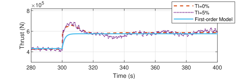
Figure 3: Thrust response of a step demanded power from 3 to 4 MW at 9 m/s with the down-regulator $\mathcal{D}$ defined in Section II-D.

For the controller design, we choose $K_{\mathrm{P}}=0$ and a damping coefficient $\zeta=0.7$, then $\omega_{\mathrm{n}}=0.446$ and $K_{\mathrm{I}}=2.947$. As is seen in Fig. 4, the integrator is sufficient to add tracking and robustness to the plant from $G$ to $L=KG$, where the disturbances are reduced and the estimation error is attenuated, as shown by $S$ and $T$. The controller provides an infinity gain margin and a phase margin of 65.2 degrees at frequency 0.047 Hz for the identified model. Up to 99% of tracking until frequencies of 0.2 Hz and at least 90.9% of reduction for frequencies greater than 7.16 Hz (from the crossover frequencies of L at $\pm$ 20 dB).

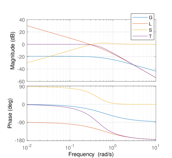
Figure 4: Bode magnitude and phase plots of L(s)=G(s)K(s), S(s) and T(s) for G(s) = 0.067625/s+0.625 and K(s)=2.947/s. The crossover frequencies 0.2 Hz and 7.16 Hz of L at +20dB and -20dB are considerable high and low, respectively. Meaning high tracking robustness and disturbance rejection [28].

The simulations were performed by feeding a reference power signal below the available power based on the normalized standard test signal [29]. The results of the thrust tracking controller are presented in Figs. 5 and 6, using an uniform wind inflow and a turbulent one, respectively. As the maximum thrust is about 512 kN by just tracking power, the thrust references were accordingly set as 500, 475, 450, 425 kN for the uniform inflow case. The results shown in Table II present a rough linear relation between the percentage of the maximum power loss and the percentage of reduction of thrust in the case studies.

TABLE II: Power loss as function of the thrust reference

Thrust	Percentage of	Maximum	Percentage of
reference	thrust reduction	power loss	power reduction
$\mathrm{[kN]}$	$[\%]$	$\mathrm{[MW]}$	$[\%]$
500	2.35	0.0750	2.1
475	7.23	0.2175	6.2
450	12.12	0.3826	10.9
425	16.99	0.5382	15.4

The proposed control architecture was able to track the computed thrust sufficiently, even though oscillations appear in the thrust force. These oscillations are due to the tower effect characterized by the blade passing frequency (3P) and to the inflow wind profile reproduced by SOWFA. They are partially accommodated by the adopted wind speed estimator and thrust computation. In addition, the proposed integral switching law presents robustness against chattering and smooth transitions.

Figure 5: Power and thrust of the simulations with no turbulence. Thrust tracking with reference of 450 kN.

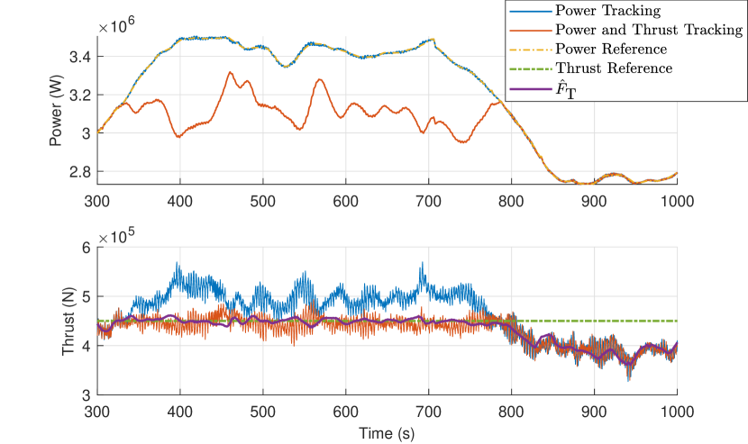
Figure 6: Power and thrust of the simulations with turbulence (turbulence intensity of 5%). Thrust tracking with reference of 450 kN

IV CONCLUSIONS

A closed-loop switching control architecture for addressing aerodynamic load constraints on wind turbines is presented. The framework makes use of down regulation and wind speed estimations. The proposed architecture effectively limits the aerodynamic loads, where the appropriate user-defined constraint would ensure safety on the system. In fact, such approaches present an undesirable loss in power production but it can be acceptable in a wind farm wide perspective. Therefore, the proposed architecture aims to prevent mechanical structures from failures and their associated costs by avoiding high stresses from the aerodynamic loads. Also, this can lead to a profit from keeping turbines operating in non-designed conditions, such as corroded structures.

Future work will focus on the development and the performance of model predictive controllers for down-regulation purposes, aiming to avoid unstable flow behaviors and oscillations in response signals, and expand the present framework to farm simulations.

References

- [1] T. Ashuri, M. Zaayer, J. Martins, G. van Bussel, and G. van Kuik, “Multidisciplinary design optimization of offshore wind turbines for minimum levelized cost of energy,” Renewable Energy, vol. 68, pp. 893–905, 2014.
- [2] H. J. Sutherland, “On the fatigue analysis of wind turbines,” Tech. Rep., 1999.
- [3] E. A. Bossanyi, “Wind turbine control for load reduction,” Wind Energy, vol. 6, no. 3, pp. 229–244, 2003.
- [4] S. J. Price and R. B. Figueira, “Corrosion protection systems and fatigue corrosion in offshore wind structures: Current status and future perspectives,” Coatings, vol. 7, no. 2, 2017.
- [5] A. May, D. McMillan, and S. Thöns, “Economic analysis of condition monitoring systems for offshore wind turbine sub-systems,” IET Renewable Power Generation, vol. 9, no. 8, pp. 900–907, 2015.
- [6] Y. Liu, R. Ferrari, P. Wu, X. Jiang, S. Li, and J.-W. van Wingerden, “Fault diagnosis of the 10mw floating offshore wind turbine benchmark: A mixed model and signal-based approach,” Renewable Energy, vol. 164, pp. 391–406, 2021.
- [7] D. T. Griffith, N. C. Yoder, B. Resor, J. White, and J. Paquette, “Structural health and prognostics management for the enhancement of offshore wind turbine operations and maintenance strategies,” Wind Energy, vol. 17, no. 11, pp. 1737–1751, 2014.
- [8] J. W. van Wingerden, L. Pao, J. Aho, and P. Fleming, “Active power control of waked wind farms,” IFAC-PapersOnLine, vol. 50, no. 1, pp. 4484 – 4491, 2017, 20th IFAC World Congress.
- [9] J. G. Silva, B. Doekemeijer, R. Ferrari, and J.-W. van Wingerden, “Active power control of waked wind farms: Compensation of turbine saturation and thrust force balance,” in 2021 European Control Conference (ECC), 2021, pp. 1223–1228.
- [10] M. Mirzaei, M. Soltani, N. K. Poulsen, and H. H. Niemann, “Model based active power control of a wind turbine,” in 2014 American Control Conference, 2014, pp. 5037–5042.
- [11] D. van der Hoek, S. Kanev, and W. Engels, “Comparison of down-regulation strategies for wind farm control and their effects on fatigue loads,” in 2018 Annual American Control Conference (ACC), 2018, pp. 3116–3121.
- [12] A. S. Deshpande and R. R. Peters, “Wind turbine controller design considerations for improved wind farm level curtailment tracking,” in 2012 IEEE Power and Energy Society General Meeting, 2012, pp. 1–6.
- [13] W. H. Lio, M. Mirzaei, and G. C. Larsen, “On wind turbine down-regulation control strategies and rotor speed set-point,” Journal of Physics: Conference Series, vol. 1037, p. 032040, jun 2018.
- [14] D. A. Juangarcia, I. Eguinoa, and T. Knudsen, “Derating a single wind farm turbine for reducing its wake and fatigue,” Journal of Physics: Conference Series, vol. 1037, p. 032039, jun 2018.
- [15] C. Santoni, U. Ciri, M. Rotea, and S. Leonardi, “Development of a high fidelity cfd code for wind farm control,” in 2015 American Control Conference (ACC), 2015, pp. 1715–1720.
- [16] K. Ma, J. Zhu, M. Soltani, A. Hajizadeh, and Z. Chen, “Wind turbine down-regulation strategy for minimum wake deficit,” in 2017 11th Asian Control Conference (ASCC), 2017, pp. 2652–2656.
- [17] J. Aho, P. Fleming, and L. Y. Pao, “Active power control of wind turbines for ancillary services: A comparison of pitch and torque control methodologies,” in 2016 American Control Conference (ACC), 2016, pp. 1407–1412.
- [18] K. Kim, H. Kim, C. Kim, I. Paek, C. Bottasso, and F. Campagnolo, “Design and validation of demanded power point tracking control algorithm of wind turbine,” Int. J. of Precision Engineering and Manufacturing-Green Technology, vol. 5, pp. 387–400, 07 2018.
- [19] J. J, S. Butterfield, W. Musial, and G. Scott, “Definition of a 5mw reference wind turbine for offshore system development,” National Renewable Energy Laboratory (NREL), 01 2009.
- [20] S. P. Mulders, M. B. Zaaijer, R. Bos, and J. W. van Wingerden, “Wind turbine control: open-source software for control education, standardization and compilation,” Journal of Physics: Conference Series, vol. 1452, p. 012010, jan 2020.
- [21] P. Fleming, J. Aho, P. Gebraad, L. Pao, and Y. Zhang, “Computational fluid dynamics simulation study of active power control in wind plants,” in 2016 American Control Conf. (ACC), 2016, pp. 1413–1420.
- [22] E. Garone, S. Di Cairano, and I. Kolmanovsky, “Reference and command governors for systems with constraints: A survey on theory and applications,” Automatica, vol. 75, pp. 306–328, 2017.
- [23] Y. Liu, A. K. Pamososuryo, R. M. G. Ferrari, and J.-W. van Wingerden, “The immersion and invariance wind speed estimator revisited and new results,” IEEE Control Systems Letters, vol. 6, pp. 361–366, 2022.
- [24] S. Laghrouche, F. Plestan, and A. Glumineau, “Higher order sliding mode control based on integral sliding mode,” Automatica, vol. 43, no. 3, pp. 531–537, 2007.
- [25] NREL, “ROSCO. Version 2.3.0,” 2021. [Online]. Available: https://github.com/NREL/rosco
- [26] M. J. Churchfield, S. Lee, J. Michalakes, and P. J. Moriarty, “A numerical study of the effects of atmospheric and wake turbulence on wind turbine dynamics,” J. of Turbulence, vol. 13, p. N14, 2012.
- [27] C. Bak, F. Zahle, R. Bitsche, T. Kim, A. Yde, L. Henriksen, M. Hansen, J. Blasques, M. Gaunaa, and A. Natarajan, “The dtu 10-mw reference wind turbine,” 2013, danish Wind Power Research 2013; Conference date: 27-05-2013 Through 28-05-2013.
- [28] S. Skogestad and I. Postlethwaite, Multivariable feedback control: Analysis and Design. Hoboken, NJ, USA: John Wiley, 2005.
- [29] C. Pilong, PJM Manual 12: Balancing Operations, 30th ed. Audubon, PA, USA: PJM, 2013.