Impacts of gravitational-wave standard siren observations from Einstein Telescope and Cosmic Explorer on weighing neutrinos in interacting dark energy models
Abstract
Multi-messenger gravitational-wave (GW) observation for binary neutron star merger events could provide a rather useful tool to explore the evolution of the universe. In particular, for the third-generation GW detectors, i.e., the Einstein Telescope (ET) and the Cosmic Explorer (CE), proposed to be built in Europe and the U.S., respectively, lots of GW standard sirens with known redshifts could be obtained, which would exert great impacts on the cosmological parameter estimation. The total neutrino mass could be measured by cosmological observations, but such a measurement is model-dependent and currently only gives an upper limit. In this work, we wish to investigate whether the GW standard sirens observed by ET and CE could help improve the constraint on the neutrino mass, in particular in the interacting dark energy (IDE) models. We find that the GW standard siren observations from ET and CE can only slightly improve the constraint on the neutrino mass in the IDE models, compared to the current limit. The improvements in the IDE models are weaker than those in the standard cosmological model. Although the limit on neutrino mass can only be slightly updated, the constraints on other cosmological parameters can be significantly improved by using the GW observations.
I Introduction
In the recent two decades, the study of cosmology has entered the era of precision cosmology. A standard model of cosmology has been established, usually called the cold dark matter (CDM) model. The measurements of cosmic microwave background (CMB) anisotropies from the Planck satellite mission have constrained the six primary parameters of the CDM model with unprecedented precision. However, with the measurement precisions of the cosmological parameters improved, some puzzling issues appeared. For example, the inferred values of the Hubble constant from the Planck observation of the CMB anisotropies (based on the CDM model) Aghanim et al. (2020) and from the Cepheid-supernova distance ladder measurement Riess et al. (2019) are inconsistent, with the tension between them more than 4 significance Riess et al. (2019). Namely, there is an inconsistency of measurements between the early and late universe, which is the so-called “Hubble tension” problem. The Hubble tension recently has been widely discussed in the literature (see, e.g., Refs. Riess (2019); Verde et al. (2019); Li et al. (2013a); Zhang et al. (2015a); Gao et al. (2021); Cai (2020); Cai et al. (2021); Zhao et al. (2017a); Guo et al. (2019, 2020); Yang et al. (2018); Yan et al. (2020); Vagnozzi (2020); Di Valentino et al. (2020a, b); Liu et al. (2020); Zhang and Huang (2020); Ding et al. (2020); Feng et al. (2020a); Lin et al. (2020); Xu and Zhang (2020); Li and Zhang (2020); Hryczuk and Jodłowski (2020); Wang et al. (2021); Vagnozzi et al. (2021); Vagnozzi (2021); Di Valentino et al. (2021); Dainotti et al. (2021); Ren et al. (2022)). Furthermore, theoretically, for the CDM model, the cosmological constant , which is equivalent to the density of vacuum energy, has always been suffering from serious theoretical challenges, such as the “fine-tuning” and “cosmic coincidence” problems Sahni and Starobinsky (2000); Bean et al. (2005). Thus, it is hard to say that the CDM model with only six base parameters is the eventual model of cosmology. All of these facts actually imply that the CDM model needs to be further extended and some extra parameters concerning new physics need to be introduced into the new models. Of course, some novel cosmological probes should also be further developed.
To extend the CDM cosmology, the primary idea is to consider the dynamical dark energy with the dark-energy density no longer a constant. In this class of models, the simplest one is the model with a dark energy having a constant equation-of-state (EoS) parameter, constant, which is usually called the CDM model. For some popular dark energy models, see, e.g., Refs. Chevallier and Polarski (2001); Linder (2003); Huterer and Turner (2001); Wetterich (2004); Jassal et al. (2005); Upadhye et al. (2005); Xia et al. (2005); Zhang (2005a); Zhang and Wu (2005); Zhang (2006); Linder (2006); Zhang and Wu (2007); Lazkoz et al. (2011); Ma and Zhang (2011); Li and Zhang (2011a, 2012); Li et al. (2012); Cai et al. (2016). There is also a class of models known as the interacting dark energy (IDE) models in which some direct, non-gravitational interaction between dark energy and dark matter is considered. The interaction between dark sectors could help resolve (or alleviate) the coincidence problem of dark energy, and also can help alleviate the Hubble tension. The IDE models have been widely studied and deeply explored till now (see, e.g., Refs. Amendola (2000, 1999); Tocchini-Valentini and Amendola (2002); Amendola and Tocchini-Valentini (2002); Comelli et al. (2003); Chimento et al. (2003); Cai and Wang (2005); Zhang et al. (2006); Ferrer et al. (2004); Zhang (2005b); Sadjadi and Alimohammadi (2006); Barrow and Clifton (2006); Sasaki et al. (2006); Abdalla et al. (2009); Bean et al. (2008); Guo et al. (2007); Zhang (2009); Caldera-Cabral et al. (2009); Valiviita et al. (2010); He et al. (2009); Koyama et al. (2009); Li et al. (2009); Xia (2009); Cai and Su (2010); Li and Zhang (2011b); Zhang et al. (2012); Xu et al. (2013); Zhang and Liu (2014); Wang et al. (2013); Salvatelli et al. (2013); Yang and Xu (2014); Wang et al. (2014); Faraoni et al. (2014); Fan et al. (2015); Yang et al. (2015); Duniya et al. (2015); Murgia et al. (2016); Costa et al. (2017); Xia and Wang (2016); Guo et al. (2017); Zhang (2017a); Feng et al. (2018); Yang et al. (2018); Guo et al. (2019); Zhao et al. (2020a); Feng et al. (2020b); Li et al. (2020a, b)).
Currently, the mainstream cosmological probes mainly include, e.g., the CMB anisotropies, baryon acoustic oscillations (BAO), type Ia supernovae (SN), direct determination of the Hubble constant (), weak gravitational lensing, redshift space distortions, and clusters of galaxies. The combinations of these cosmological data based on the electromagnetic (EM) observations have provided precise measurements for the base cosmological parameters. But for some extended parameters beyond the standard CDM model, e.g., the EoS parameter of dark energy, the tensor-to-scalar ratio, and the total mass of neutrinos, they still cannot be precisely measured. Therefore, on one hand, the EM observations should be further greatly developed, and on the other hand, some novel cosmological probes are also needed to be developed in the future. In the next few decades, the gravitational-wave (GW) standard siren observation is one of the most promising cosmological probes.
The detection of the GW event GW170817 Abbott et al. (2017a) from the binary neutron star (BNS) merger initiated the multi-messenger astronomy era. Because in this event, not only GWs but also the EM signals in various bands were detected for the same transient source Abbott et al. (2017b, c). From the analysis of the waveform of GW, one can obtain the absolute luminosity distance to the source. Furthermore, the redshift of the source can also be determined by identifying the EM counterpart of the GW source. With the known distance and redshift of a celestial source, a distance–redshift relation can be established, which can be used to explore the expansion history of the universe Schutz (1986). Such a tool of exploring the evolution of the universe provided by GWs is called “standard sirens” (note here that the case having EM counterparts is usually referred to as bright sirens, to be differentiated with the case of dark sirens without EM counterparts) Holz and Hughes (2005).
The main advantage of the GW standard siren method is that the absolute luminosity distances can be measured. This is obviously superior to the SN observation, in that the latter can only measure the ratio of luminosity distances at different redshifts. In addition, the GW observation can observe much higher redshift events, compared to the SN observation.
It is indisputable that the GW standard siren will be developed into a powerful cosmological probe in the future. The third-generation (3G) ground-based GW detectors, such as the Einstein Telescope (ET) ET- ; Punturo et al. (2010) in Europe and the Cosmic Explorer (CE) CE- ; Abbott et al. (2017d) in the United States, have been proposed. In the 2030s, ET will be brought into operation. CE will start its observation in the mid-2030s. The 3G ground-based GW detectors have a much wider detection-frequency range and a much better detection sensitivity, which can observe much more BNS events at much deeper redshifts. Recently, the GW standard sirens have been widely discussed in the literature Cai and Yang (2017); Cai et al. (2018a); Cai and Yang (2018); Zhang (2019); Zhao et al. (2018a); Du et al. (2019); Cai et al. (2018b); Yang et al. (2020, 2019); Bachega et al. (2020); Chang et al. (2019); He (2019); Liu et al. (2018a); Berti et al. (2018); Liu et al. (2018b); Will (1994); Zhao et al. (2020b); Wang et al. (2022a); Qi et al. (2021); Jin et al. (2021); Buchmuller et al. (2020); Borhanian and Sathyaprakash (2022); Colgáin (2022); Zhu et al. (2022); de Souza et al. (2022); Wang et al. (2022b); Jin et al. (2022); Wu et al. (2022) (see Ref. Bian et al. (2021) for a recent review). It is found that the GW standard siren observations from ET and CE would play an important role in the cosmological parameter estimation Zhang et al. (2020a, 2019a); Wang et al. (2018a); Zhang et al. (2019b); Li et al. (2020c); Jin et al. (2020).
In cosmology, neutrinos play a crucial role in helping shape the large-scale structure and the expansion history of the universe. The phenomenon of neutrino oscillation indicates that neutrinos have masses and there are mass splittings between different neutrino species. However, it is extremely difficult to measure the absolute masses of neutrinos. Neutrino oscillation experiments cannot measure the absolute neutrino masses, but can only give the squared mass differences between the different mass eigenstates of neutrinos. The solar and reactor experiments give and the atmospheric and accelerator beam experiments give Olive et al. (2014); Xing (2020). Thus, there are two possible mass hierarchies of the neutrino mass spectrum, namely, the normal hierarchy (NH) with and the inverted hierarchy (IH) with . In addition, in some cases one also considers the cosmological models of neglecting the neutrino mass splittings, namely , which is usually called the degenerate hierarchy (DH).
Although the neutrino masses can hardly be measured by particle physics experiments, they can be effectively constrained by the cosmological observations. This is because massive neutrinos can exert some impacts on the evolution of the universe. Using the current cosmological observations, an upper limit on the total neutrino mass can be obtained. So far, the most stringent limit on the total neutrino mass comes from the Planck 2018 CMB observation, and the combination CMB+BAO+SN gives the CL upper limit eV, for the DH case in the CDM model. See e.g. Refs. Hu et al. (1998); Reid et al. (2010); Thomas et al. (2010); Carbone et al. (2011); Huo et al. (2012); Wang et al. (2012); Li et al. (2013b); Audren et al. (2013); Riemer-Sørensen et al. (2014); Font-Ribera et al. (2014); Zhang et al. (2014a, b); Zhou and He (2014); Ade et al. (2016); Zhang et al. (2015b); Geng et al. (2016); Lu et al. (2016); Kumar and Nunes (2016); Xu and Huang (2018); Vagnozzi et al. (2017); Zhang (2017b); Zhao et al. (2018b); Vagnozzi et al. (2018); Li et al. (2018); Wang et al. (2018b); Feng et al. (2019); Zhao et al. (2017b); Zhang (2016); Huang et al. (2016); Wang et al. (2016); Giusarma et al. (2016); Allahverdi et al. (2017); Gariazzo et al. (2018); Roy Choudhury and Choubey (2018); Han et al. (2017); Zhang et al. (2020b); Diaz Rivero et al. (2019); Zhang et al. (2020c) for studies on neutrino mass in cosmology.
In a recent forecast Wang et al. (2018a), it was shown that the standard sirens observed by the ET can be used to improve the constraints on the total neutrino mass in the CDM model. Using 1000 GW standard siren data points of the BNS merger events, it is found that the upper limits on can be tightened by about Wang et al. (2018a). However, weighing neutrinos in cosmology depends on the cosmological model considered, and thus one would be curious about whether the role the GW data play in helping measure the neutrino mass will change if an extension to the CDM model is considered. In this work, we consider the IDE models, and we wish to see what will happen on measuring neutrino mass when the IDE models are considered.
In an IDE model, the energy conservation equations for dark energy and CDM satisfy
| (1) | |||
| (2) |
where is the energy transfer rate, and represent the energy densities of dark energy and CDM, respectively, is the Hubble parameter, and a dot represents the derivative with respect to the cosmic time . In this work, we consider the interaction form of , where is a dimensionless coupling parameter. Here, and means CDM decaying into dark energy and dark energy decaying into CDM, respectively.
In this work, we consider the IDE versions of the CDM and CDM models, which are called the ICDM and ICDM models. We will discuss the cosmological parameter estimation in the ICDM+ and ICDM+ models. Moreover, we will consider the three neutrino mass hierarchy cases, i.e., the NH, IH, DH cases. To avoid the perturbation divergence problem in the IDE models, in this work we employ the extended parameterized post-Friedmann (ePPF) framework Li et al. (2014a, b) to calculate the perturbations of dark energy.
We simulate the GW standard siren data observed by ET and CE, and we use these simulated GW data to investigate how well they can be used to improve the constraints on the neutrino mass as well as other cosmological parameters on the basis of the current CMB+BAO+SN constraints.
The rest of this paper is organized as follows. In Sec. II.1, we introduce the methods of simulating the GW standard siren data. In Sec. II.2 we describe the EM cosmological observations used in this work. In Sec. II.3, we briefly describe the methods of constraining cosmological parameters. In Sec. III, we give the constraint results and make some relevant discussions. The conclusion is given in Sec. IV.
II Method and data
In this section, we first introduce the method of simulating the GW standard siren data from ET and CE. Then, we describe the current mainstream EM cosmological observations used in this work. Finally, we briefly introduce the method of constraining cosmological parameters.
II.1 Simulation of the GW standard sirens
The primary GW sources in the detection frequency band of the ground-based GW detectors are the mergers of BNS, binary stellar-mass black hole (BBH), and so on. The BNS mergers could produce rich EM signals Li and Paczynski (1998) that can be detected by the EM observatories, thus enabling precise redshift measurements. Owing to the fact that there are no EM signals produced in the process of the BBH mergers, their redshifts could not be precisely measured through the detection of the EM counterparts. Hence, in this work, we only simulate the GW standard sirens from the BNS mergers.
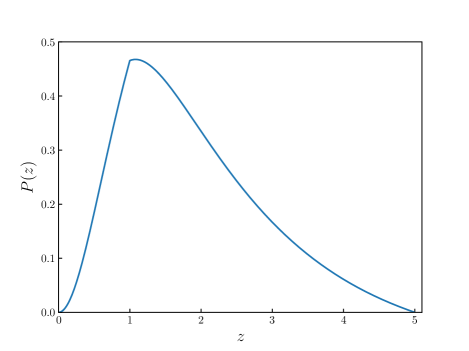
Following Refs. Zhao et al. (2011); Cai and Yang (2017), the redshift distribution of the BNS mergers takes the form
| (3) |
where is the comoving distance at the redshift , and represents the redshift evolution of the burst rate, which takes the form Schneider et al. (2001); Cutler and Holz (2009); Cai and Yang (2017)
| (4) |
In Fig. 1, we show the redshift distribution of BNS mergers.
Considering the transverse-traceless gauge, the strain in the GW interferometers can be described by two independent polarization amplitudes, and ,
| (5) |
where and are the antenna response functions, and describe the location of the GW source relative to the GW detector, and is the polarization angle.
The antenna response functions of ET are Zhao et al. (2011)
| (6) |
Since ET has three interferometers with inclined angles between each other, the other two response functions are and .
For CE, the antenna response functions are
| (7) |
We consider the waveform in the inspiralling stage for a non-spinning BNS system. Here we adopt the restricted post-Newtonian (PN) approximation and calculate the waveform to the 3.5 PN order Sathyaprakash and Schutz (2009); Blanchet and Iyer (2005),
| (8) |
where the Fourier amplitude is given by
| (9) |
where is the observed chirp mass, is the total mass of the coalescing binary system with and being the component masses, is the symmetric mass ratio, is the luminosity distance to the GW source, is the inclination angle between the binary’s orbital angular momentum and the line of sight, is the coalescence time, and is the coalescence phase. The definitions of the functions and can refer to Refs. Sathyaprakash and Schutz (2009); Blanchet and Iyer (2005).
The signal-to-noise ratio (SNR) for the network of (i.e., = 3 for ET and = 1 for CE) independent interferometers can be calculated by
| (10) |
where . The inner product is defined as
| (11) |
where is the lower cutoff frequency ( Hz for ET and Hz for CE), is the frequency at the last stable orbit with Zhao et al. (2011), and is the one-side noise power spectral density (PSD). We adopt PSD of ET from Ref. ETc and that of CE from Ref. CEc . In this work, we choose the threshold of SNR to be 8 in our simulation.
For the 3G ground-based GW detectors, a few BNS merger events per year could be detected, but only about 0.1% of them may have -ray bursts toward us Yu et al. (2021). Recently, in Ref. Chen et al. (2021) Chen et al. made a forecast and showed that 910 GW standard siren events could be observed by a 10-year observation of CE and Swift++. Therefore, in our forecast in the present work, for ET and CE, we simulate 1000 GW standard sirens from BNS mergers based on the 10-year observation.
We consider three measurement errors of , consisting of the instrumental error , the weak-lensing error , and the peculiar velocity error . Therefore, the total error of is
| (12) |
We first use the Fisher information matrix to calculate . For a GW event, when using Fisher information matrix to estimate , we consider a Fisher information matrix consisting of nine parameters of a GW source (, , , , , , , , ), and thus the correlations between the nine parameters are considered in the analysis. For a network of independent interferometers, the Fisher information matrix can be written as
| (13) |
with given by
| (14) |
where denotes nine parameters (, , , , , , , , ) for a GW event. Then we have
| (15) |
where is the total Fisher information matrix for the network of interferometers. Note that here .
The error caused by weak lensing is adopted from Refs. Hirata et al. (2010); Speri et al. (2021),
| (16) |
Here, we consider a delensing factor . We use dedicated matter surveys along the line of sight of the GW event in order to estimate the lensing magnification distribution, which can remove part of the uncertainty due to weak lensing. This reduces the weak lensing uncertainty. The delensing factor is given by
| (17) |
The error caused by the peculiar velocity of the GW source is given by Kocsis et al. (2006)
| (18) |
where is the Hubble parameter. is the peculiar velocity of the GW source and we roughly set .
For each simulated GW source, the sky location, the binary inclination, the coalescence phase, and the polarization angle are randomly chosen in the ranges of , , , , and . The mass of an NS is randomly chosen in the range of . Without loss of generality, the merger time is chosen to in our analysis. Here we wish to note that the inclination angle should be randomly chosen in the range of when simulating isotropic GW sources. However, in this work, we simulate GW events by detecting short -ray bursts (SGRBs) to determine sources’ redshifts. Owing to the fact that SGRBs are strongly beamed Rezzolla et al. (2011), the detectable inclination angle is about Li (2015); Yu et al. (2021). Hence, in the present work, we set the inclination angle to be in the range of . This is an ideal treatment, but for this work, since the number of simulated GW standard sirens is fixed, it has little effect on showing the impact of GW standard sirens on breaking cosmological parameter degeneracies and improving constraints on the cosmological parameters.
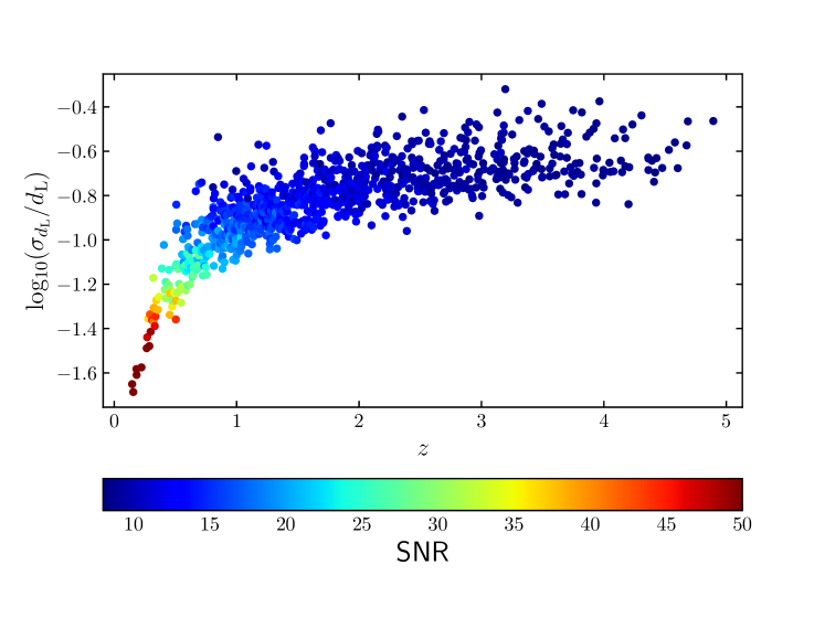
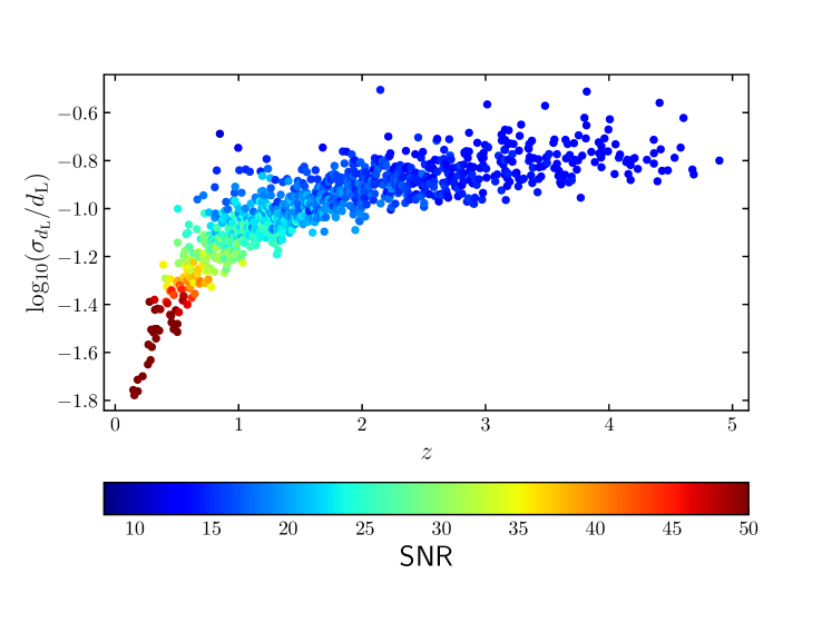
In Fig. 2, we show the scatter plot of the simulated standard siren data from ET (upper panel) and CE (lower panel).222Here we wish to note that in the colorbars of Fig. 2, we set the maximum value to be 50, i.e., a GW event with SNR greater than 50 has the same color as the GW event with SNR of 50. In fact, many red dots have SNRs greater than 50, e.g., SNR at for ET is 105.9, while for CE is 158.2. The reason of the design is that we can better highlight the comparison between ET and CE from the figure. If we set the maximal value of SNR higher (to about 100), almost all the data points are in blue, so it is difficult to visually compare SNRs of the two detectors from the figure. We can see that: (i) the total errors of from CE are smaller than those from ET; (ii) SNR of CE is higher than that of ET at the same redshift.
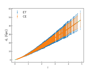
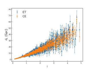
In Fig. 3, we show the simulated GW standard sirens from ET and CE. In the left panel, we show the standard siren data points without Gaussian randomness, where the central value of the luminosity distance is calculated by the fiducial cosmological model. In the right panel, in order to reflect the fluctuations in measured values resulting from actual observations, we show the standard siren data points with Gaussian randomization (the central values are populated according to a Gaussian distribution with mean being and standard deviation being ). In principle, the right panel is more representative of actual observational data, but the central values of have no effect on determining the absolute errors of cosmological parameters. Therefore, we use the data points in the left panel to constrain the cosmological models, because this is more helpful in investigating how the parameter degeneracies are broken to improve measurement precisions of cosmological parameters. We can clearly see that the measurement errors of from CE are smaller than those from ET, because CE has a better sensitivity than ET.
II.2 Other cosmological observations
In this work, we consider three current mainstream EM cosmological observations, including CMB, BAO, and SN. For the CMB data, we consider the Planck TT, TE, EE spectra at , the low- temperature Commander likelihood, and the low- SimAll EE likelihood from the Planck 2018 release Aghanim et al. (2020). For the BAO data, we consider the measurements from 6dFGS () Beutler et al. (2011), SDSS-MGS () Ross et al. (2015), and BOSS DR12 (, 0.51, and 0.61) Alam et al. (2017). For the SN data, we use the latest Pantheon sample, which is comprised of 1048 data points from the Pantheon compilation Scolnic et al. (2018).
II.3 Method of constraining cosmological parameters
To resolve the large-scale instability problem in the IDE cosmology Valiviita et al. (2008), we apply the ePPF approach Li et al. (2014a, b) for the IDE scenario so that the whole parameter space of IDE models can be explored without any divergence of the dark-energy perturbation. In this work, we employ the modified version of the available Markov-Chain Monte Carlo package CosmoMC Lewis and Bridle (2002), with the ePPF code Li et al. (2014a, b) inserted, to constrain the neutrino mass and other cosmological parameters. In order to show the impacts of GW data from CE and ET on constraining cosmological parameters, we use CMB+BAO+SN, CMB+BAO+SN+ET, and CMB+BAO+SN+CE to make our analysis. For convenience, we use CBS to standard for CMB+BAO+SN in the following.
For the GW standard siren observation with data points, the function can be written as
| (19) |
where , , and are the th GW event’s redshift, luminosity distance, and the measurement error of the luminosity distance, respectively. represents the set of cosmological parameters.
When considering the combination of the current EM observations and the GW standard siren observations, the total function is
| (20) |
| CDM | CMB+BAO+SN | CMB+BAO+SN+ET | CMB+BAO+SN+CE | |||||||||
|---|---|---|---|---|---|---|---|---|---|---|---|---|
| Parameter | NH | IH | DH | NH | IH | DH | NH | IH | DH | |||
| [eV] | ||||||||||||
| ICDM | CMB+BAO+SN | CMB+BAO+SN+ET | CMB+BAO+SN+CE | |||||||||
|---|---|---|---|---|---|---|---|---|---|---|---|---|
| Parameter | NH | IH | DH | NH | IH | DH | NH | IH | DH | |||
| [eV] | ||||||||||||
| ICDM | CMB+BAO+SN | CMB+BAO+SN+ET | CMB+BAO+SN+CE | |||||||||
|---|---|---|---|---|---|---|---|---|---|---|---|---|
| Parameter | NH | IH | DH | NH | IH | DH | NH | IH | DH | |||
| [eV] | ||||||||||||
III Results and discussion
In this section, we report the constraint results of cosmological parameters in the CDM+, ICDM+, and ICDM+ models. In these models, the three mass hierarchy cases of neutrinos, i.e., the NH, IH, and DH cases, have been considered. The constraint results of the NH case are shown as a representative in Figs. 4–6 and the constraint results are summarized in Tables 1–3. Note that for the constraints on the total neutrino mass, the upper limits are given. Note also that using the squared mass differences derived from the neutrino oscillation experiments, one can obtain the lower limits for the total neutrino mass, i.e., 0.05 eV for NH and 0.1 eV for IH; in the case of DH, the smallest value of the total neutrino mass is zero. For a parameter , we use and to represent its absolute and relative errors, respectively, with defined as .
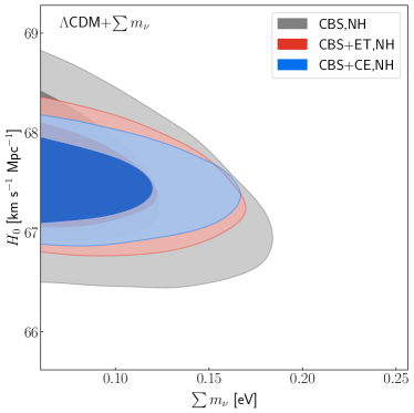
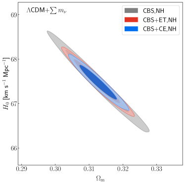
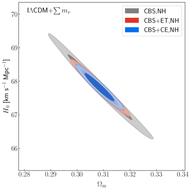
We first take a look at the results in the CDM+ model. In Fig. 4, we show the constraints on the CDM+ model in the – and – planes from the CBS, CBS+ET, and CBS+CE data. We find that the addition of the GW data to the CBS data could lead to the reduction of the upper limits of to some extent. The CBS+CE data give slightly smaller upper limits on than those from the CBS+ET data. Concretely, when adding the ET data to the CBS data, the upper limits on could be reduced by 2.7%–12.4% in the three hierarchy cases. While for CE, the upper limits on could be reduced by 4.3%–14.0% in the three hierarchy cases. Here the results of ET are consistent with the previous results in Ref. Wang et al. (2018a).
Although using the GW data could only slightly improve the limits on the neutrino mass, they can significantly help improve the constraints on other cosmological parameters. We find that the constraints on and could be improved by 29.0%–32.8% and 30.4%–34.7%, respectively, when adding the ET data to the CBS data, and by 40.3%–43.8% and 43.5%–46.9%, respectively, for the case of CE.
In Fig. 5, we show the constraints on the ICDM+ model in the – and – planes from the CBS, CBS+ET, and CBS+CE data. We can clearly see that, when considering the interaction between vacuum energy and dark matter, the improvement of the limits on by adding GW data is rather not evident. In the case of ET, the improvement of the limit on is only 0.7%–1.8%, and in the case of CE, the improvement is 1.8%–4.1%. Therefore, we find that compared with the standard CDM model, in its interaction version, the ICDM model, the improvement of the limits on by GW data from ET and CE becomes weaker. This is because the ICDM model considers an extra cosmological parameter compared with the CDM model, which will degenerate with other cosmological parameters when the CBS data are used to constrain the ICDM model. Hence, compared with the CDM model, the addition of the GW data to the CBS data for its interaction version leads to weaker improvement.
We also find that the constraints on the coupling parameter can be improved by using the GW data to a certain extent. In the ICDM+ model, the constraints on are improved by 19.2%–20.8% and 22.3%–26.2%, respectively, when the GW data of ET and CE are added on the basis of the CBS case.
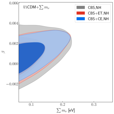
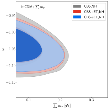
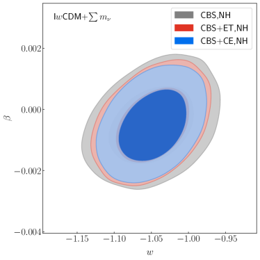
In Fig. 6, we show the constraints on the ICDM+ model in the – and – planes from the CBS, CBS+ET, and CBS+CE data. We find that in this case the improvement of the limits on the neutrino mass is better than in the previous case. For ET, the improvement of the limit on is 2.0%–5.4%, and for CE, the improvement is 5.3%–8.7%.
We find that in this case the constraints on the coupling parameter and the EoS parameter of dark energy can both be significantly improved by considering the addition of GW data. The constraints on and are improved by 2.4%–8.0% and 10.8%–13.2%, respectively, when considering the ET data, and by 7.1%–10.2% and 18.9%–21.1%, respectively, when considering the CE data.
In this work, we discuss the cosmological constraints on the IDE models in the cases of considering the GW standard siren observations from 3G ground-based GW detectors ET and CE. The results show that the limits on the neutrino mass can only be slightly improved with the help of the GW data, on the basis of the CBS constraint. Since the GW data can precisely constrain the Hubble constant , the addition of them in the cosmological fit can help break the cosmological parameter degeneracies formed by other cosmological observations. Therefore, the consideration of GW standard siren data can help significantly improve the constraints on the most cosmological parameters. However, the effect of massive neutrinos in the late universe and on the large scales cannot be distinctively distinguished from that of the cold dark matter, leading to the improvement of the limits on the neutrino mass by considering GW data is not obvious. Anyway, even though the impact on constraining the neutrino mass is not apparent, the GW standard sirens are rather useful in helping improve the constraints on the most cosmological parameters including the EoS of dark energy and the coupling between dark energy and dark matter.
IV Conclusion
In the era of 3G ground-based GW detectors, a lot of GW standard siren data with the know redshifts could be obtained by the multi-messenger observation for BNS merger events. Obviously, these standard sirens would exert great impacts on the cosmological parameter estimation. Since the GW standard sirens can tightly constrain the Hubble constant, the consideration of them in a joint cosmological fit can lead to the cosmological parameter degeneracies formed by other cosmological observations being well broken. The GW standard sirens can thus be used to help significantly improve the constraints on cosmological parameters in the future.
It is of great interest to investigate whether the limits on the total neutrino mass can also be effectively improved by considering the GW standard siren data. In particular, the cosmological constraints on the neutrino mass are strongly model-dependent, and so the cases in different cosmological scenarios are needed to be detailedly discussed. In this work, we discuss the issue of weighing neutrinos in the IDE models by using the GW standard siren observations by ET and CE.
We consider the simplest IDE models, namely the ICDM and ICDM models with . We simulate the GW standard siren data of the BNS mergers observed by ET and CE (in a way of multi-messenger detection). We investigate whether the GW standard sirens observed by ET and CE could help improve the constraint on the neutrino mass in the IDE models.
It is found that the GW standard siren observations from ET and CE can only slightly improve the constraint on the neutrino mass in the IDE models, compared to the current limit given by CMB+BAO+SN. This is mainly because the effect of massive neutrinos in the late universe and on the large scales cannot be distinctively distinguished from that of the CDM, leading to the improvement of the limits on the neutrino mass by considering GW data is not obvious. Although the limit on neutrino mass can only be slightly updated by considering the GW standard sirens, they are fairly useful in helping improve the constraints on the most cosmological parameters including the EoS of dark energy and the coupling between dark energy and dark matter.
Acknowledgements.
This work was supported by the National Natural Science Foundation of China (Grants Nos. 11975072, 11835009, 11875102, and 11690021), the Liaoning Revitalization Talents Program (Grant No. XLYC1905011), the Fundamental Research Funds for the Central Universities (Grant No. N2005030), the National 111 Project of China (Grant No. B16009), and the Science Research Grants from the China Manned Space Project (Grant No. CMS-CSST-2021-B01).References
- Aghanim et al. (2020) N. Aghanim et al. (Planck), Planck 2018 results. VI. Cosmological parameters, Astron. Astrophys. 641, A6 (2020), arXiv:1807.06209 [astro-ph.CO] .
- Riess et al. (2019) A. G. Riess, S. Casertano, W. Yuan, L. M. Macri, and D. Scolnic, Large Magellanic Cloud Cepheid Standards Provide a 1% Foundation for the Determination of the Hubble Constant and Stronger Evidence for Physics beyond CDM, Astrophys. J. 876, 85 (2019), arXiv:1903.07603 [astro-ph.CO] .
- Riess (2019) A. G. Riess, The Expansion of the Universe is Faster than Expected, Nature Rev. Phys. 2, 10 (2019), arXiv:2001.03624 [astro-ph.CO] .
- Verde et al. (2019) L. Verde, T. Treu, and A. G. Riess, Tensions between the Early and the Late Universe, Nature Astron. 3, 891 (2019), arXiv:1907.10625 [astro-ph.CO] .
- Li et al. (2013a) M. Li, X.-D. Li, Y.-Z. Ma, X. Zhang, and Z. Zhang, Planck Constraints on Holographic Dark Energy, JCAP 09, 021, arXiv:1305.5302 [astro-ph.CO] .
- Zhang et al. (2015a) J.-F. Zhang, Y.-H. Li, and X. Zhang, Sterile neutrinos help reconcile the observational results of primordial gravitational waves from Planck and BICEP2, Phys. Lett. B 740, 359 (2015a), arXiv:1403.7028 [astro-ph.CO] .
- Gao et al. (2021) L.-Y. Gao, Z.-W. Zhao, S.-S. Xue, and X. Zhang, Relieving the H 0 tension with a new interacting dark energy model, JCAP 07, 005, arXiv:2101.10714 [astro-ph.CO] .
- Cai (2020) R.-G. Cai, Editorial, Sci. China Phys. Mech. Astron. 63, 290401 (2020).
- Cai et al. (2021) R.-G. Cai, Z.-K. Guo, L. Li, S.-J. Wang, and W.-W. Yu, Chameleon dark energy can resolve the Hubble tension, Phys. Rev. D 103, 121302 (2021), arXiv:2102.02020 [astro-ph.CO] .
- Zhao et al. (2017a) M.-M. Zhao, D.-Z. He, J.-F. Zhang, and X. Zhang, Search for sterile neutrinos in holographic dark energy cosmology: Reconciling Planck observation with the local measurement of the Hubble constant, Phys. Rev. D 96, 043520 (2017a), arXiv:1703.08456 [astro-ph.CO] .
- Guo et al. (2019) R.-Y. Guo, J.-F. Zhang, and X. Zhang, Can the tension be resolved in extensions to CDM cosmology?, JCAP 02, 054, arXiv:1809.02340 [astro-ph.CO] .
- Guo et al. (2020) R.-Y. Guo, J.-F. Zhang, and X. Zhang, Inflation model selection revisited after a 1.91% measurement of the Hubble constant, Sci. China Phys. Mech. Astron. 63, 290406 (2020), arXiv:1910.13944 [astro-ph.CO] .
- Yang et al. (2018) W. Yang, S. Pan, E. Di Valentino, R. C. Nunes, S. Vagnozzi, and D. F. Mota, Tale of stable interacting dark energy, observational signatures, and the tension, JCAP 09, 019, arXiv:1805.08252 [astro-ph.CO] .
- Yan et al. (2020) S.-F. Yan, P. Zhang, J.-W. Chen, X.-Z. Zhang, Y.-F. Cai, and E. N. Saridakis, Interpreting cosmological tensions from the effective field theory of torsional gravity, Phys. Rev. D 101, 121301 (2020), arXiv:1909.06388 [astro-ph.CO] .
- Vagnozzi (2020) S. Vagnozzi, New physics in light of the tension: An alternative view, Phys. Rev. D 102, 023518 (2020), arXiv:1907.07569 [astro-ph.CO] .
- Di Valentino et al. (2020a) E. Di Valentino, A. Melchiorri, O. Mena, and S. Vagnozzi, Nonminimal dark sector physics and cosmological tensions, Phys. Rev. D 101, 063502 (2020a), arXiv:1910.09853 [astro-ph.CO] .
- Di Valentino et al. (2020b) E. Di Valentino, A. Melchiorri, O. Mena, and S. Vagnozzi, Interacting dark energy in the early 2020s: A promising solution to the and cosmic shear tensions, Phys. Dark Univ. 30, 100666 (2020b), arXiv:1908.04281 [astro-ph.CO] .
- Liu et al. (2020) M. Liu, Z. Huang, X. Luo, H. Miao, N. K. Singh, and L. Huang, Can Non-standard Recombination Resolve the Hubble Tension?, Sci. China Phys. Mech. Astron. 63, 290405 (2020), arXiv:1912.00190 [astro-ph.CO] .
- Zhang and Huang (2020) X. Zhang and Q.-G. Huang, Measuring H0 from low-z datasets, Sci. China Phys. Mech. Astron. 63, 290402 (2020), arXiv:1911.09439 [astro-ph.CO] .
- Ding et al. (2020) Q. Ding, T. Nakama, and Y. Wang, A gigaparsec-scale local void and the Hubble tension, Sci. China Phys. Mech. Astron. 63, 290403 (2020), arXiv:1912.12600 [astro-ph.CO] .
- Feng et al. (2020a) L. Feng, D.-Z. He, H.-L. Li, J.-F. Zhang, and X. Zhang, Constraints on active and sterile neutrinos in an interacting dark energy cosmology, Sci. China Phys. Mech. Astron. 63, 290404 (2020a), arXiv:1910.03872 [astro-ph.CO] .
- Lin et al. (2020) M.-X. Lin, W. Hu, and M. Raveri, Testing in Acoustic Dark Energy with Planck and ACT Polarization, Phys. Rev. D 102, 123523 (2020), arXiv:2009.08974 [astro-ph.CO] .
- Xu and Zhang (2020) Y. Xu and X. Zhang, Cosmological parameter measurement and neutral hydrogen 21 cm sky survey with the Square Kilometre Array, Sci. China Phys. Mech. Astron. 63, 270431 (2020), arXiv:2002.00572 [astro-ph.CO] .
- Li and Zhang (2020) H. Li and X. Zhang, A novel method of measuring cosmological distances using broad-line regions of quasars, Sci. Bull. 65, 1419 (2020), arXiv:2005.10458 [astro-ph.CO] .
- Hryczuk and Jodłowski (2020) A. Hryczuk and K. Jodłowski, Self-interacting dark matter from late decays and the tension, Phys. Rev. D 102, 043024 (2020), arXiv:2006.16139 [hep-ph] .
- Wang et al. (2021) L.-F. Wang, J.-H. Zhang, D.-Z. He, J.-F. Zhang, and X. Zhang, Constraints on interacting dark energy models from time-delay cosmography with seven lensed quasars, (2021), arXiv:2102.09331 [astro-ph.CO] .
- Vagnozzi et al. (2021) S. Vagnozzi, F. Pacucci, and A. Loeb, Implications for the Hubble tension from the ages of the oldest astrophysical objects, (2021), arXiv:2105.10421 [astro-ph.CO] .
- Vagnozzi (2021) S. Vagnozzi, Consistency tests of CDM from the early integrated Sachs-Wolfe effect: Implications for early-time new physics and the Hubble tension, Phys. Rev. D 104, 063524 (2021), arXiv:2105.10425 [astro-ph.CO] .
- Di Valentino et al. (2021) E. Di Valentino, O. Mena, S. Pan, L. Visinelli, W. Yang, A. Melchiorri, D. F. Mota, A. G. Riess, and J. Silk, In the realm of the Hubble tension—a review of solutions, Class. Quant. Grav. 38, 153001 (2021), arXiv:2103.01183 [astro-ph.CO] .
- Dainotti et al. (2021) M. G. Dainotti, B. De Simone, T. Schiavone, G. Montani, E. Rinaldi, and G. Lambiase, On the Hubble constant tension in the SNe Ia Pantheon sample, Astrophys. J. 912, 150 (2021), arXiv:2103.02117 [astro-ph.CO] .
- Ren et al. (2022) X. Ren, S.-F. Yan, Y. Zhao, Y.-F. Cai, and E. N. Saridakis, Gaussian processes and effective field theory of gravity under the tension, (2022), arXiv:2203.01926 [astro-ph.CO] .
- Sahni and Starobinsky (2000) V. Sahni and A. A. Starobinsky, The Case for a positive cosmological Lambda term, Int. J. Mod. Phys. D 9, 373 (2000), arXiv:astro-ph/9904398 .
- Bean et al. (2005) R. Bean, S. M. Carroll, and M. Trodden, Insights into dark energy: interplay between theory and observation, (2005), arXiv:astro-ph/0510059 .
- Chevallier and Polarski (2001) M. Chevallier and D. Polarski, Accelerating universes with scaling dark matter, Int. J. Mod. Phys. D 10, 213 (2001), arXiv:gr-qc/0009008 .
- Linder (2003) E. V. Linder, Exploring the expansion history of the universe, Phys. Rev. Lett. 90, 091301 (2003), arXiv:astro-ph/0208512 .
- Huterer and Turner (2001) D. Huterer and M. S. Turner, Probing the dark energy: Methods and strategies, Phys. Rev. D 64, 123527 (2001), arXiv:astro-ph/0012510 .
- Wetterich (2004) C. Wetterich, Phenomenological parameterization of quintessence, Phys. Lett. B 594, 17 (2004), arXiv:astro-ph/0403289 .
- Jassal et al. (2005) H. K. Jassal, J. S. Bagla, and T. Padmanabhan, WMAP constraints on low redshift evolution of dark energy, Mon. Not. Roy. Astron. Soc. 356, L11 (2005), arXiv:astro-ph/0404378 .
- Upadhye et al. (2005) A. Upadhye, M. Ishak, and P. J. Steinhardt, Dynamical dark energy: Current constraints and forecasts, Phys. Rev. D 72, 063501 (2005), arXiv:astro-ph/0411803 .
- Xia et al. (2005) J.-Q. Xia, B. Feng, and X.-M. Zhang, Constraints on oscillating quintom from supernova, microwave background and galaxy clustering, Mod. Phys. Lett. A 20, 2409 (2005), arXiv:astro-ph/0411501 .
- Zhang (2005a) X. Zhang, Statefinder diagnostic for holographic dark energy model, Int. J. Mod. Phys. D 14, 1597 (2005a), arXiv:astro-ph/0504586 .
- Zhang and Wu (2005) X. Zhang and F.-Q. Wu, Constraints on holographic dark energy from Type Ia supernova observations, Phys. Rev. D 72, 043524 (2005), arXiv:astro-ph/0506310 .
- Zhang (2006) X. Zhang, Dynamical vacuum energy, holographic quintom, and the reconstruction of scalar-field dark energy, Phys. Rev. D 74, 103505 (2006), arXiv:astro-ph/0609699 .
- Linder (2006) E. V. Linder, The paths of quintessence, Phys. Rev. D 73, 063010 (2006), arXiv:astro-ph/0601052 .
- Zhang and Wu (2007) X. Zhang and F.-Q. Wu, Constraints on Holographic Dark Energy from Latest Supernovae, Galaxy Clustering, and Cosmic Microwave Background Anisotropy Observations, Phys. Rev. D 76, 023502 (2007), arXiv:astro-ph/0701405 .
- Lazkoz et al. (2011) R. Lazkoz, V. Salzano, and I. Sendra, Oscillations in the dark energy EoS: new MCMC lessons, Phys. Lett. B 694, 198 (2011), arXiv:1003.6084 [astro-ph.CO] .
- Ma and Zhang (2011) J.-Z. Ma and X. Zhang, Probing the dynamics of dark energy with novel parametrizations, Phys. Lett. B 699, 233 (2011), arXiv:1102.2671 [astro-ph.CO] .
- Li and Zhang (2011a) H. Li and X. Zhang, Probing the dynamics of dark energy with divergence-free parametrizations: A global fit study, Phys. Lett. B 703, 119 (2011a), arXiv:1106.5658 [astro-ph.CO] .
- Li and Zhang (2012) H. Li and X. Zhang, Constraining dynamical dark energy with a divergence-free parametrization in the presence of spatial curvature and massive neutrinos, Phys. Lett. B 713, 160 (2012), arXiv:1202.4071 [astro-ph.CO] .
- Li et al. (2012) X.-D. Li, S. Wang, Q.-G. Huang, X. Zhang, and M. Li, Dark Energy and Fate of the Universe, Sci. China Phys. Mech. Astron. 55, 1330 (2012), arXiv:1202.4060 [astro-ph.CO] .
- Cai et al. (2016) Y.-F. Cai, S. Capozziello, M. De Laurentis, and E. N. Saridakis, f(T) teleparallel gravity and cosmology, Rept. Prog. Phys. 79, 106901 (2016), arXiv:1511.07586 [gr-qc] .
- Amendola (2000) L. Amendola, Coupled quintessence, Phys. Rev. D 62, 043511 (2000), arXiv:astro-ph/9908023 .
- Amendola (1999) L. Amendola, Scaling solutions in general nonminimal coupling theories, Phys. Rev. D 60, 043501 (1999), arXiv:astro-ph/9904120 .
- Tocchini-Valentini and Amendola (2002) D. Tocchini-Valentini and L. Amendola, Stationary dark energy with a baryon dominated era: Solving the coincidence problem with a linear coupling, Phys. Rev. D 65, 063508 (2002), arXiv:astro-ph/0108143 .
- Amendola and Tocchini-Valentini (2002) L. Amendola and D. Tocchini-Valentini, Baryon bias and structure formation in an accelerating universe, Phys. Rev. D 66, 043528 (2002), arXiv:astro-ph/0111535 .
- Comelli et al. (2003) D. Comelli, M. Pietroni, and A. Riotto, Dark energy and dark matter, Phys. Lett. B 571, 115 (2003), arXiv:hep-ph/0302080 .
- Chimento et al. (2003) L. P. Chimento, A. S. Jakubi, D. Pavon, and W. Zimdahl, Interacting quintessence solution to the coincidence problem, Phys. Rev. D 67, 083513 (2003), arXiv:astro-ph/0303145 .
- Cai and Wang (2005) R.-G. Cai and A. Wang, Cosmology with interaction between phantom dark energy and dark matter and the coincidence problem, JCAP 03, 002, arXiv:hep-th/0411025 .
- Zhang et al. (2006) X. Zhang, F.-Q. Wu, and J. Zhang, A New generalized Chaplygin gas as a scheme for unification of dark energy and dark matter, JCAP 01, 003, arXiv:astro-ph/0411221 .
- Ferrer et al. (2004) F. Ferrer, S. Rasanen, and J. Valiviita, Correlated isocurvature perturbations from mixed inflaton-curvaton decay, JCAP 10, 010, arXiv:astro-ph/0407300 .
- Zhang (2005b) X. Zhang, Statefinder diagnostic for coupled quintessence, Phys. Lett. B 611, 1 (2005b), arXiv:astro-ph/0503075 .
- Sadjadi and Alimohammadi (2006) H. M. Sadjadi and M. Alimohammadi, Cosmological coincidence problem in interactive dark energy models, Phys. Rev. D 74, 103007 (2006), arXiv:gr-qc/0610080 .
- Barrow and Clifton (2006) J. D. Barrow and T. Clifton, Cosmologies with energy exchange, Phys. Rev. D 73, 103520 (2006), arXiv:gr-qc/0604063 .
- Sasaki et al. (2006) M. Sasaki, J. Valiviita, and D. Wands, Non-Gaussianity of the primordial perturbation in the curvaton model, Phys. Rev. D 74, 103003 (2006), arXiv:astro-ph/0607627 .
- Abdalla et al. (2009) E. Abdalla, L. R. W. Abramo, L. Sodre, Jr., and B. Wang, Signature of the interaction between dark energy and dark matter in galaxy clusters, Phys. Lett. B 673, 107 (2009), arXiv:0710.1198 [astro-ph] .
- Bean et al. (2008) R. Bean, E. E. Flanagan, and M. Trodden, Adiabatic instability in coupled dark energy-dark matter models, Phys. Rev. D 78, 023009 (2008), arXiv:0709.1128 [astro-ph] .
- Guo et al. (2007) Z.-K. Guo, N. Ohta, and S. Tsujikawa, Probing the Coupling between Dark Components of the Universe, Phys. Rev. D 76, 023508 (2007), arXiv:astro-ph/0702015 .
- Zhang (2009) X. Zhang, Holographic Ricci dark energy: Current observational constraints, quintom feature, and the reconstruction of scalar-field dark energy, Phys. Rev. D 79, 103509 (2009), arXiv:0901.2262 [astro-ph.CO] .
- Caldera-Cabral et al. (2009) G. Caldera-Cabral, R. Maartens, and B. M. Schaefer, The Growth of Structure in Interacting Dark Energy Models, JCAP 07, 027, arXiv:0905.0492 [astro-ph.CO] .
- Valiviita et al. (2010) J. Valiviita, R. Maartens, and E. Majerotto, Observational constraints on an interacting dark energy model, Mon. Not. Roy. Astron. Soc. 402, 2355 (2010), arXiv:0907.4987 [astro-ph.CO] .
- He et al. (2009) J.-H. He, B. Wang, and Y. P. Jing, Effects of dark sectors’ mutual interaction on the growth of structures, JCAP 07, 030, arXiv:0902.0660 [gr-qc] .
- Koyama et al. (2009) K. Koyama, R. Maartens, and Y.-S. Song, Velocities as a probe of dark sector interactions, JCAP 10, 017, arXiv:0907.2126 [astro-ph.CO] .
- Li et al. (2009) M. Li, X.-D. Li, S. Wang, Y. Wang, and X. Zhang, Probing interaction and spatial curvature in the holographic dark energy model, JCAP 12, 014, arXiv:0910.3855 [astro-ph.CO] .
- Xia (2009) J.-Q. Xia, Constraint on coupled dark energy models from observations, Phys. Rev. D 80, 103514 (2009), arXiv:0911.4820 [astro-ph.CO] .
- Cai and Su (2010) R.-G. Cai and Q. Su, On the Dark Sector Interactions, Phys. Rev. D 81, 103514 (2010), arXiv:0912.1943 [astro-ph.CO] .
- Li and Zhang (2011b) Y.-H. Li and X. Zhang, Running coupling: Does the coupling between dark energy and dark matter change sign during the cosmological evolution?, Eur. Phys. J. C 71, 1700 (2011b), arXiv:1103.3185 [astro-ph.CO] .
- Zhang et al. (2012) Z. Zhang, S. Li, X.-D. Li, X. Zhang, and M. Li, Revisit of the Interaction between Holographic Dark Energy and Dark Matter, JCAP 06, 009, arXiv:1204.6135 [astro-ph.CO] .
- Xu et al. (2013) X.-D. Xu, B. Wang, P. Zhang, and F. Atrio-Barandela, The effect of Dark Matter and Dark Energy interactions on the peculiar velocity field and the kinetic Sunyaev-Zel’dovich effect, JCAP 12, 001, arXiv:1308.1475 [astro-ph.CO] .
- Zhang and Liu (2014) M.-J. Zhang and W.-B. Liu, Observational constraint on the interacting dark energy models including the Sandage-Loeb test, Eur. Phys. J. C 74, 2863 (2014), arXiv:1312.0224 [astro-ph.CO] .
- Wang et al. (2013) Y. Wang, D. Wands, L. Xu, J. De-Santiago, and A. Hojjati, Cosmological constraints on a decomposed Chaplygin gas, Phys. Rev. D 87, 083503 (2013), arXiv:1301.5315 [astro-ph.CO] .
- Salvatelli et al. (2013) V. Salvatelli, A. Marchini, L. Lopez-Honorez, and O. Mena, New constraints on Coupled Dark Energy from the Planck satellite experiment, Phys. Rev. D 88, 023531 (2013), arXiv:1304.7119 [astro-ph.CO] .
- Yang and Xu (2014) W. Yang and L. Xu, Testing coupled dark energy with large scale structure observation, JCAP 08, 034, arXiv:1401.5177 [astro-ph.CO] .
- Wang et al. (2014) S. Wang, Y.-Z. Wang, J.-J. Geng, and X. Zhang, Effects of time-varying in SNLS3 on constraining interacting dark energy models, Eur. Phys. J. C 74, 3148 (2014), arXiv:1406.0072 [astro-ph.CO] .
- Faraoni et al. (2014) V. Faraoni, J. B. Dent, and E. N. Saridakis, Covariantizing the interaction between dark energy and dark matter, Phys. Rev. D 90, 063510 (2014), arXiv:1405.7288 [gr-qc] .
- Fan et al. (2015) Y. Fan, P. Wu, and H. Yu, Cosmological perturbations of non-minimally coupled quintessence in the metric and Palatini formalisms, Phys. Lett. B 746, 230 (2015).
- Yang et al. (2015) T. Yang, Z.-K. Guo, and R.-G. Cai, Reconstructing the interaction between dark energy and dark matter using Gaussian Processes, Phys. Rev. D 91, 123533 (2015), arXiv:1505.04443 [astro-ph.CO] .
- Duniya et al. (2015) D. G. A. Duniya, D. Bertacca, and R. Maartens, Probing the imprint of interacting dark energy on very large scales, Phys. Rev. D 91, 063530 (2015), arXiv:1502.06424 [astro-ph.CO] .
- Murgia et al. (2016) R. Murgia, S. Gariazzo, and N. Fornengo, Constraints on the Coupling between Dark Energy and Dark Matter from CMB data, JCAP 04, 014, arXiv:1602.01765 [astro-ph.CO] .
- Costa et al. (2017) A. A. Costa, X.-D. Xu, B. Wang, and E. Abdalla, Constraints on interacting dark energy models from Planck 2015 and redshift-space distortion data, JCAP 01, 028, arXiv:1605.04138 [astro-ph.CO] .
- Xia and Wang (2016) D.-M. Xia and S. Wang, Constraining interacting dark energy models with latest cosmological observations, Mon. Not. Roy. Astron. Soc. 463, 952 (2016), arXiv:1608.04545 [astro-ph.CO] .
- Guo et al. (2017) R.-Y. Guo, Y.-H. Li, J.-F. Zhang, and X. Zhang, Weighing neutrinos in the scenario of vacuum energy interacting with cold dark matter: application of the parameterized post-Friedmann approach, JCAP 05, 040, arXiv:1702.04189 [astro-ph.CO] .
- Zhang (2017a) X. Zhang, Probing the interaction between dark energy and dark matter with the parametrized post-Friedmann approach, Sci. China Phys. Mech. Astron. 60, 050431 (2017a), arXiv:1702.04564 [astro-ph.CO] .
- Feng et al. (2018) L. Feng, Y.-H. Li, F. Yu, J.-F. Zhang, and X. Zhang, Exploring interacting holographic dark energy in a perturbed universe with parameterized post-Friedmann approach, Eur. Phys. J. C 78, 865 (2018), arXiv:1807.03022 [astro-ph.CO] .
- Zhao et al. (2020a) M. Zhao, R. Guo, D. He, J. Zhang, and X. Zhang, Dark energy versus modified gravity: Impacts on measuring neutrino mass, Sci. China Phys. Mech. Astron. 63, 230412 (2020a), arXiv:1810.11658 [astro-ph.CO] .
- Feng et al. (2020b) L. Feng, H.-L. Li, J.-F. Zhang, and X. Zhang, Exploring neutrino mass and mass hierarchy in interacting dark energy models, Sci. China Phys. Mech. Astron. 63, 220401 (2020b), arXiv:1903.08848 [astro-ph.CO] .
- Li et al. (2020a) C. Li, X. Ren, M. Khurshudyan, and Y.-F. Cai, Implications of the possible 21-cm line excess at cosmic dawn on dynamics of interacting dark energy, Phys. Lett. B 801, 135141 (2020a), arXiv:1904.02458 [astro-ph.CO] .
- Li et al. (2020b) H.-L. Li, J.-F. Zhang, and X. Zhang, Constraints on neutrino mass in the scenario of vacuum energy interacting with cold dark matter after Planck 2018, Commun. Theor. Phys. 72, 125401 (2020b), arXiv:2005.12041 [astro-ph.CO] .
- Abbott et al. (2017a) B. P. Abbott et al. (LIGO Scientific, Virgo), GW170817: Observation of Gravitational Waves from a Binary Neutron Star Inspiral, Phys. Rev. Lett. 119, 161101 (2017a), arXiv:1710.05832 [gr-qc] .
- Abbott et al. (2017b) B. P. Abbott et al. (LIGO Scientific, Virgo, Fermi-GBM, INTEGRAL), Gravitational Waves and Gamma-rays from a Binary Neutron Star Merger: GW170817 and GRB 170817A, Astrophys. J. Lett. 848, L13 (2017b), arXiv:1710.05834 [astro-ph.HE] .
- Abbott et al. (2017c) B. P. Abbott et al. (LIGO Scientific, Virgo, Fermi GBM, INTEGRAL, IceCube, AstroSat Cadmium Zinc Telluride Imager Team, IPN, Insight-Hxmt, ANTARES, Swift, AGILE Team, 1M2H Team, Dark Energy Camera GW-EM, DES, DLT40, GRAWITA, Fermi-LAT, ATCA, ASKAP, Las Cumbres Observatory Group, OzGrav, DWF (Deeper Wider Faster Program), AST3, CAASTRO, VINROUGE, MASTER, J-GEM, GROWTH, JAGWAR, CaltechNRAO, TTU-NRAO, NuSTAR, Pan-STARRS, MAXI Team, TZAC Consortium, KU, Nordic Optical Telescope, ePESSTO, GROND, Texas Tech University, SALT Group, TOROS, BOOTES, MWA, CALET, IKI-GW Follow-up, H.E.S.S., LOFAR, LWA, HAWC, Pierre Auger, ALMA, Euro VLBI Team, Pi of Sky, Chandra Team at McGill University, DFN, ATLAS Telescopes, High Time Resolution Universe Survey, RIMAS, RATIR, SKA South Africa/MeerKAT), Multi-messenger Observations of a Binary Neutron Star Merger, Astrophys. J. Lett. 848, L12 (2017c), arXiv:1710.05833 [astro-ph.HE] .
- Schutz (1986) B. F. Schutz, Determining the Hubble Constant from Gravitational Wave Observations, Nature 323, 310 (1986).
- Holz and Hughes (2005) D. E. Holz and S. A. Hughes, Using gravitational-wave standard sirens, Astrophys. J. 629, 15 (2005), arXiv:astro-ph/0504616 .
- (103) ET, https://www.et-gw.eu/.
- Punturo et al. (2010) M. Punturo et al., The Einstein Telescope: A third-generation gravitational wave observatory, Class. Quant. Grav. 27, 194002 (2010).
- (105) CE, https://cosmicexplorer.org/.
- Abbott et al. (2017d) B. P. Abbott et al. (LIGO Scientific), Exploring the Sensitivity of Next Generation Gravitational Wave Detectors, Class. Quant. Grav. 34, 044001 (2017d), arXiv:1607.08697 [astro-ph.IM] .
- Cai and Yang (2017) R.-G. Cai and T. Yang, Estimating cosmological parameters by the simulated data of gravitational waves from the Einstein Telescope, Phys. Rev. D 95, 044024 (2017), arXiv:1608.08008 [astro-ph.CO] .
- Cai et al. (2018a) R.-G. Cai, T.-B. Liu, X.-W. Liu, S.-J. Wang, and T. Yang, Probing cosmic anisotropy with gravitational waves as standard sirens, Phys. Rev. D 97, 103005 (2018a), arXiv:1712.00952 [astro-ph.CO] .
- Cai and Yang (2018) R.-G. Cai and T. Yang, Standard sirens and dark sector with Gaussian process, EPJ Web Conf. 168, 01008 (2018), arXiv:1709.00837 [astro-ph.CO] .
- Zhang (2019) X. Zhang, Gravitational wave standard sirens and cosmological parameter measurement, Sci. China Phys. Mech. Astron. 62, 110431 (2019), arXiv:1905.11122 [astro-ph.CO] .
- Zhao et al. (2018a) W. Zhao, B. S. Wright, and B. Li, Constraining the time variation of Newton’s constant with gravitational-wave standard sirens and supernovae, JCAP 10, 052, arXiv:1804.03066 [astro-ph.CO] .
- Du et al. (2019) M. Du, W. Yang, L. Xu, S. Pan, and D. F. Mota, Future constraints on dynamical dark-energy using gravitational-wave standard sirens, Phys. Rev. D 100, 043535 (2019), arXiv:1812.01440 [astro-ph.CO] .
- Cai et al. (2018b) Y.-F. Cai, C. Li, E. N. Saridakis, and L. Xue, gravity after GW170817 and GRB170817A, Phys. Rev. D 97, 103513 (2018b), arXiv:1801.05827 [gr-qc] .
- Yang et al. (2020) W. Yang, S. Pan, E. Di Valentino, B. Wang, and A. Wang, Forecasting interacting vacuum-energy models using gravitational waves, JCAP 05, 050, arXiv:1904.11980 [astro-ph.CO] .
- Yang et al. (2019) W. Yang, S. Vagnozzi, E. Di Valentino, R. C. Nunes, S. Pan, and D. F. Mota, Listening to the sound of dark sector interactions with gravitational wave standard sirens, JCAP 07, 037, arXiv:1905.08286 [astro-ph.CO] .
- Bachega et al. (2020) R. R. A. Bachega, A. A. Costa, E. Abdalla, and K. S. F. Fornazier, Forecasting the Interaction in Dark Matter-Dark Energy Models with Standard Sirens From the Einstein Telescope, JCAP 05, 021, arXiv:1906.08909 [astro-ph.CO] .
- Chang et al. (2019) Z. Chang, Q.-G. Huang, S. Wang, and Z.-C. Zhao, Low-redshift constraints on the Hubble constant from the baryon acoustic oscillation “standard rulers” and the gravitational wave “standard sirens”, Eur. Phys. J. C 79, 177 (2019).
- He (2019) J.-h. He, Accurate method to determine the systematics due to the peculiar velocities of galaxies in measuring the Hubble constant from gravitational-wave standard sirens, Phys. Rev. D 100, 023527 (2019), arXiv:1903.11254 [astro-ph.CO] .
- Liu et al. (2018a) T. Liu, X. Zhang, and W. Zhao, Constraining gravity in solar system, cosmology and binary pulsar systems, Phys. Lett. B 777, 286 (2018a), arXiv:1711.08991 [astro-ph.CO] .
- Berti et al. (2018) E. Berti, K. Yagi, and N. Yunes, Extreme Gravity Tests with Gravitational Waves from Compact Binary Coalescences: (I) Inspiral-Merger, Gen. Rel. Grav. 50, 46 (2018), arXiv:1801.03208 [gr-qc] .
- Liu et al. (2018b) T. Liu, X. Zhang, W. Zhao, K. Lin, C. Zhang, S. Zhang, X. Zhao, T. Zhu, and A. Wang, Waveforms of compact binary inspiral gravitational radiation in screened modified gravity, Phys. Rev. D 98, 083023 (2018b), arXiv:1806.05674 [gr-qc] .
- Will (1994) C. M. Will, Testing scalar - tensor gravity with gravitational wave observations of inspiraling compact binaries, Phys. Rev. D 50, 6058 (1994), arXiv:gr-qc/9406022 .
- Zhao et al. (2020b) Z.-W. Zhao, L.-F. Wang, J.-F. Zhang, and X. Zhang, Prospects for improving cosmological parameter estimation with gravitational-wave standard sirens from Taiji, Sci. Bull. 65, 1340 (2020b), arXiv:1912.11629 [astro-ph.CO] .
- Wang et al. (2022a) L.-F. Wang, S.-J. Jin, J.-F. Zhang, and X. Zhang, Forecast for cosmological parameter estimation with gravitational-wave standard sirens from the LISA-Taiji network, Sci. China Phys. Mech. Astron. 65, 210411 (2022a), arXiv:2101.11882 [gr-qc] .
- Qi et al. (2021) J.-Z. Qi, S.-J. Jin, X.-L. Fan, J.-F. Zhang, and X. Zhang, Using a multi-messenger and multi-wavelength observational strategy to probe the nature of dark energy through direct measurements of cosmic expansion history, JCAP 12 (12), 042, arXiv:2102.01292 [astro-ph.CO] .
- Jin et al. (2021) S.-J. Jin, L.-F. Wang, P.-J. Wu, J.-F. Zhang, and X. Zhang, How can gravitational-wave standard sirens and 21-cm intensity mapping jointly provide a precise late-universe cosmological probe?, Phys. Rev. D 104, 103507 (2021), arXiv:2106.01859 [astro-ph.CO] .
- Buchmuller et al. (2020) W. Buchmuller, V. Domcke, H. Murayama, and K. Schmitz, Probing the scale of grand unification with gravitational waves, Phys. Lett. B 809, 135764 (2020), arXiv:1912.03695 [hep-ph] .
- Borhanian and Sathyaprakash (2022) S. Borhanian and B. S. Sathyaprakash, Listening to the Universe with Next Generation Ground-Based Gravitational-Wave Detectors, (2022), arXiv:2202.11048 [gr-qc] .
- Colgáin (2022) E. O. Colgáin, Probing the Anisotropic Universe with Gravitational Waves (2022) arXiv:2203.03956 [astro-ph.CO] .
- Zhu et al. (2022) L.-G. Zhu, L.-H. Xie, Y.-M. Hu, S. Liu, E.-K. Li, N. R. Napolitano, B.-T. Tang, J.-d. Zhang, and J. Mei, Constraining the Hubble constant to a precision of about 1% using multi-band dark standard siren detections, Sci. China Phys. Mech. Astron. 65, 259811 (2022), arXiv:2110.05224 [astro-ph.CO] .
- de Souza et al. (2022) J. M. S. de Souza, R. Sturani, and J. Alcaniz, Cosmography with standard sirens from the Einstein Telescope, JCAP 03 (03), 025, arXiv:2110.13316 [gr-qc] .
- Wang et al. (2022b) L.-F. Wang, G.-P. Zhang, Y. Shao, and X. Zhang, Achieving precision cosmology with gravitational-wave bright sirens from SKA-era pulsar timing arrays, (2022b), arXiv:2201.00607 [astro-ph.CO] .
- Jin et al. (2022) S.-J. Jin, T.-N. Li, J.-F. Zhang, and X. Zhang, Precisely measuring the Hubble constant and dark energy using only gravitational-wave dark sirens, (2022), arXiv:2202.11882 [gr-qc] .
- Wu et al. (2022) P.-J. Wu, Y. Shao, S.-J. Jin, and X. Zhang, A path to precision cosmology: Synergy between four promising late-universe cosmological probes, (2022), arXiv:2202.09726 [astro-ph.CO] .
- Bian et al. (2021) L. Bian et al., The Gravitational-wave physics II: Progress, Sci. China Phys. Mech. Astron. 64, 120401 (2021), arXiv:2106.10235 [gr-qc] .
- Zhang et al. (2020a) J.-F. Zhang, H.-Y. Dong, J.-Z. Qi, and X. Zhang, Prospect for constraining holographic dark energy with gravitational wave standard sirens from the Einstein Telescope, Eur. Phys. J. C 80, 217 (2020a), arXiv:1906.07504 [astro-ph.CO] .
- Zhang et al. (2019a) X.-N. Zhang, L.-F. Wang, J.-F. Zhang, and X. Zhang, Improving cosmological parameter estimation with the future gravitational-wave standard siren observation from the Einstein Telescope, Phys. Rev. D 99, 063510 (2019a), arXiv:1804.08379 [astro-ph.CO] .
- Wang et al. (2018a) L.-F. Wang, X.-N. Zhang, J.-F. Zhang, and X. Zhang, Impacts of gravitational-wave standard siren observation of the Einstein Telescope on weighing neutrinos in cosmology, Phys. Lett. B 782, 87 (2018a), arXiv:1802.04720 [astro-ph.CO] .
- Zhang et al. (2019b) J.-F. Zhang, M. Zhang, S.-J. Jin, J.-Z. Qi, and X. Zhang, Cosmological parameter estimation with future gravitational wave standard siren observation from the Einstein Telescope, JCAP 09, 068, arXiv:1907.03238 [astro-ph.CO] .
- Li et al. (2020c) H.-L. Li, D.-Z. He, J.-F. Zhang, and X. Zhang, Quantifying the impacts of future gravitational-wave data on constraining interacting dark energy, JCAP 06, 038, arXiv:1908.03098 [astro-ph.CO] .
- Jin et al. (2020) S.-J. Jin, D.-Z. He, Y. Xu, J.-F. Zhang, and X. Zhang, Forecast for cosmological parameter estimation with gravitational-wave standard siren observation from the Cosmic Explorer, JCAP 03, 051, arXiv:2001.05393 [astro-ph.CO] .
- Olive et al. (2014) K. A. Olive et al. (Particle Data Group), Review of Particle Physics, Chin. Phys. C 38, 090001 (2014).
- Xing (2020) Z.-z. Xing, Flavor structures of charged fermions and massive neutrinos, Phys. Rept. 854, 1 (2020), arXiv:1909.09610 [hep-ph] .
- Hu et al. (1998) W. Hu, D. J. Eisenstein, and M. Tegmark, Weighing neutrinos with galaxy surveys, Phys. Rev. Lett. 80, 5255 (1998), arXiv:astro-ph/9712057 .
- Reid et al. (2010) B. A. Reid, L. Verde, R. Jimenez, and O. Mena, Robust Neutrino Constraints by Combining Low Redshift Observations with the CMB, JCAP 01, 003, arXiv:0910.0008 [astro-ph.CO] .
- Thomas et al. (2010) S. A. Thomas, F. B. Abdalla, and O. Lahav, Upper Bound of 0.28eV on the Neutrino Masses from the Largest Photometric Redshift Survey, Phys. Rev. Lett. 105, 031301 (2010), arXiv:0911.5291 [astro-ph.CO] .
- Carbone et al. (2011) C. Carbone, L. Verde, Y. Wang, and A. Cimatti, Neutrino constraints from future nearly all-sky spectroscopic galaxy surveys, JCAP 03, 030, arXiv:1012.2868 [astro-ph.CO] .
- Huo et al. (2012) Y. Huo, T. Li, Y. Liao, D. V. Nanopoulos, and Y. Qi, Constraints on Neutrino Velocities Revisited, Phys. Rev. D 85, 034022 (2012), arXiv:1112.0264 [hep-ph] .
- Wang et al. (2012) X. Wang, X.-L. Meng, T.-J. Zhang, H. Shan, Y. Gong, C. Tao, X. Chen, and Y. F. Huang, Observational constraints on cosmic neutrinos and dark energy revisited, JCAP 11, 018, arXiv:1210.2136 [astro-ph.CO] .
- Li et al. (2013b) Y.-H. Li, S. Wang, X.-D. Li, and X. Zhang, Holographic dark energy in a Universe with spatial curvature and massive neutrinos: a full Markov Chain Monte Carlo exploration, JCAP 02, 033, arXiv:1207.6679 [astro-ph.CO] .
- Audren et al. (2013) B. Audren, J. Lesgourgues, S. Bird, M. G. Haehnelt, and M. Viel, Neutrino masses and cosmological parameters from a Euclid-like survey: Markov Chain Monte Carlo forecasts including theoretical errors, JCAP 01, 026, arXiv:1210.2194 [astro-ph.CO] .
- Riemer-Sørensen et al. (2014) S. Riemer-Sørensen, D. Parkinson, and T. M. Davis, Combining Planck data with large scale structure information gives a strong neutrino mass constraint, Phys. Rev. D 89, 103505 (2014), arXiv:1306.4153 [astro-ph.CO] .
- Font-Ribera et al. (2014) A. Font-Ribera, P. McDonald, N. Mostek, B. A. Reid, H.-J. Seo, and A. Slosar, DESI and other dark energy experiments in the era of neutrino mass measurements, JCAP 05, 023, arXiv:1308.4164 [astro-ph.CO] .
- Zhang et al. (2014a) J.-F. Zhang, Y.-H. Li, and X. Zhang, Cosmological constraints on neutrinos after BICEP2, Eur. Phys. J. C 74, 2954 (2014a), arXiv:1404.3598 [astro-ph.CO] .
- Zhang et al. (2014b) J.-F. Zhang, J.-J. Geng, and X. Zhang, Neutrinos and dark energy after Planck and BICEP2: data consistency tests and cosmological parameter constraints, JCAP 10, 044, arXiv:1408.0481 [astro-ph.CO] .
- Zhou and He (2014) X.-Y. Zhou and J.-H. He, Weighing neutrinos in gravity in light of BICEP2, Commun. Theor. Phys. 62, 102 (2014), arXiv:1406.6822 [astro-ph.CO] .
- Ade et al. (2016) P. A. R. Ade et al. (Planck), Planck 2015 results. XIII. Cosmological parameters, Astron. Astrophys. 594, A13 (2016), arXiv:1502.01589 [astro-ph.CO] .
- Zhang et al. (2015b) J.-F. Zhang, M.-M. Zhao, Y.-H. Li, and X. Zhang, Neutrinos in the holographic dark energy model: constraints from latest measurements of expansion history and growth of structure, JCAP 04, 038, arXiv:1502.04028 [astro-ph.CO] .
- Geng et al. (2016) C.-Q. Geng, C.-C. Lee, R. Myrzakulov, M. Sami, and E. N. Saridakis, Observational constraints on varying neutrino-mass cosmology, JCAP 01, 049, arXiv:1504.08141 [astro-ph.CO] .
- Lu et al. (2016) J. Lu, M. Liu, Y. Wu, Y. Wang, and W. Yang, Cosmic constraint on massive neutrinos in viable gravity with producing CDM background expansion, Eur. Phys. J. C 76, 679 (2016), arXiv:1606.02987 [astro-ph.CO] .
- Kumar and Nunes (2016) S. Kumar and R. C. Nunes, Probing the interaction between dark matter and dark energy in the presence of massive neutrinos, Phys. Rev. D 94, 123511 (2016), arXiv:1608.02454 [astro-ph.CO] .
- Xu and Huang (2018) L. Xu and Q.-G. Huang, Detecting the Neutrinos Mass Hierarchy from Cosmological Data, Sci. China Phys. Mech. Astron. 61, 039521 (2018), arXiv:1611.05178 [astro-ph.CO] .
- Vagnozzi et al. (2017) S. Vagnozzi, E. Giusarma, O. Mena, K. Freese, M. Gerbino, S. Ho, and M. Lattanzi, Unveiling secrets with cosmological data: neutrino masses and mass hierarchy, Phys. Rev. D 96, 123503 (2017), arXiv:1701.08172 [astro-ph.CO] .
- Zhang (2017b) X. Zhang, Weighing neutrinos in dynamical dark energy models, Sci. China Phys. Mech. Astron. 60, 060431 (2017b), arXiv:1703.00651 [astro-ph.CO] .
- Zhao et al. (2018b) M.-M. Zhao, J.-F. Zhang, and X. Zhang, Measuring growth index in a universe with massive neutrinos: A revisit of the general relativity test with the latest observations, Phys. Lett. B 779, 473 (2018b), arXiv:1710.02391 [astro-ph.CO] .
- Vagnozzi et al. (2018) S. Vagnozzi, S. Dhawan, M. Gerbino, K. Freese, A. Goobar, and O. Mena, Constraints on the sum of the neutrino masses in dynamical dark energy models with are tighter than those obtained in CDM, Phys. Rev. D 98, 083501 (2018), arXiv:1801.08553 [astro-ph.CO] .
- Li et al. (2018) E.-K. Li, H. Zhang, M. Du, Z.-H. Zhou, and L. Xu, Probing the Neutrino Mass Hierarchy beyond CDM Model, JCAP 08, 042, arXiv:1703.01554 [astro-ph.CO] .
- Wang et al. (2018b) S. Wang, Y.-F. Wang, and D.-M. Xia, Constraints on the sum of neutrino masses using cosmological data including the latest extended Baryon Oscillation Spectroscopic Survey DR14 quasar sample, Chin. Phys. C 42, 065103 (2018b), arXiv:1707.00588 [astro-ph.CO] .
- Feng et al. (2019) L. Feng, J.-F. Zhang, and X. Zhang, Search for sterile neutrinos in a universe of vacuum energy interacting with cold dark matter, Phys. Dark Univ. 23, 100261 (2019), arXiv:1712.03148 [astro-ph.CO] .
- Zhao et al. (2017b) M.-M. Zhao, Y.-H. Li, J.-F. Zhang, and X. Zhang, Constraining neutrino mass and extra relativistic degrees of freedom in dynamical dark energy models using Planck 2015 data in combination with low-redshift cosmological probes: basic extensions to CDM cosmology, Mon. Not. Roy. Astron. Soc. 469, 1713 (2017b), arXiv:1608.01219 [astro-ph.CO] .
- Zhang (2016) X. Zhang, Impacts of dark energy on weighing neutrinos after Planck 2015, Phys. Rev. D 93, 083011 (2016), arXiv:1511.02651 [astro-ph.CO] .
- Huang et al. (2016) Q.-G. Huang, K. Wang, and S. Wang, Constraints on the neutrino mass and mass hierarchy from cosmological observations, Eur. Phys. J. C 76, 489 (2016), arXiv:1512.05899 [astro-ph.CO] .
- Wang et al. (2016) S. Wang, Y.-F. Wang, D.-M. Xia, and X. Zhang, Impacts of dark energy on weighing neutrinos: mass hierarchies considered, Phys. Rev. D 94, 083519 (2016), arXiv:1608.00672 [astro-ph.CO] .
- Giusarma et al. (2016) E. Giusarma, M. Gerbino, O. Mena, S. Vagnozzi, S. Ho, and K. Freese, Improvement of cosmological neutrino mass bounds, Phys. Rev. D 94, 083522 (2016), arXiv:1605.04320 [astro-ph.CO] .
- Allahverdi et al. (2017) R. Allahverdi, Y. Gao, B. Knockel, and S. Shalgar, Indirect Signals from Solar Dark Matter Annihilation to Long-lived Right-handed Neutrinos, Phys. Rev. D 95, 075001 (2017), arXiv:1612.03110 [hep-ph] .
- Gariazzo et al. (2018) S. Gariazzo, M. Archidiacono, P. F. de Salas, O. Mena, C. A. Ternes, and M. Tórtola, Neutrino masses and their ordering: Global Data, Priors and Models, JCAP 03, 011, arXiv:1801.04946 [hep-ph] .
- Roy Choudhury and Choubey (2018) S. Roy Choudhury and S. Choubey, Updated Bounds on Sum of Neutrino Masses in Various Cosmological Scenarios, JCAP 09, 017, arXiv:1806.10832 [astro-ph.CO] .
- Han et al. (2017) J. Han, R. Wang, W. Wang, and X.-N. Wei, Neutrino mass matrices with one texture equality and one vanishing neutrino mass, Phys. Rev. D 96, 075043 (2017), arXiv:1705.05725 [hep-ph] .
- Zhang et al. (2020b) J.-F. Zhang, B. Wang, and X. Zhang, Forecast for weighing neutrinos in cosmology with SKA, Sci. China Phys. Mech. Astron. 63, 280411 (2020b), arXiv:1907.00179 [astro-ph.CO] .
- Diaz Rivero et al. (2019) A. Diaz Rivero, V. Miranda, and C. Dvorkin, Observable Predictions for Massive-Neutrino Cosmologies with Model-Independent Dark Energy, Phys. Rev. D 100, 063504 (2019), arXiv:1903.03125 [astro-ph.CO] .
- Zhang et al. (2020c) M. Zhang, J.-F. Zhang, and X. Zhang, Impacts of dark energy on constraining neutrino mass after Planck 2018, Commun. Theor. Phys. 72, 125402 (2020c), arXiv:2005.04647 [astro-ph.CO] .
- Li et al. (2014a) Y.-H. Li, J.-F. Zhang, and X. Zhang, Parametrized Post-Friedmann Framework for Interacting Dark Energy, Phys. Rev. D 90, 063005 (2014a), arXiv:1404.5220 [astro-ph.CO] .
- Li et al. (2014b) Y.-H. Li, J.-F. Zhang, and X. Zhang, Exploring the full parameter space for an interacting dark energy model with recent observations including redshift-space distortions: Application of the parametrized post-Friedmann approach, Phys. Rev. D 90, 123007 (2014b), arXiv:1409.7205 [astro-ph.CO] .
- Li and Paczynski (1998) L.-X. Li and B. Paczynski, Transient events from neutron star mergers, Astrophys. J. Lett. 507, L59 (1998), arXiv:astro-ph/9807272 .
- Zhao et al. (2011) W. Zhao, C. Van Den Broeck, D. Baskaran, and T. G. F. Li, Determination of Dark Energy by the Einstein Telescope: Comparing with CMB, BAO and SNIa Observations, Phys. Rev. D 83, 023005 (2011), arXiv:1009.0206 [astro-ph.CO] .
- Schneider et al. (2001) R. Schneider, V. Ferrari, S. Matarrese, and S. F. Portegies Zwart, Gravitational waves from cosmological compact binaries, Mon. Not. Roy. Astron. Soc. 324, 797 (2001), arXiv:astro-ph/0002055 .
- Cutler and Holz (2009) C. Cutler and D. E. Holz, Ultra-high precision cosmology from gravitational waves, Phys. Rev. D 80, 104009 (2009), arXiv:0906.3752 [astro-ph.CO] .
- Sathyaprakash and Schutz (2009) B. S. Sathyaprakash and B. F. Schutz, Physics, Astrophysics and Cosmology with Gravitational Waves, Living Rev. Rel. 12, 2 (2009), arXiv:0903.0338 [gr-qc] .
- Blanchet and Iyer (2005) L. Blanchet and B. R. Iyer, Hadamard regularization of the third post-Newtonian gravitational wave generation of two point masses, Phys. Rev. D 71, 024004 (2005), arXiv:gr-qc/0409094 .
- (190) https://www.et-gw.eu/index.php/etsensitivities/.
- (191) https://cosmicexplorer.org/sensitivity.html.
- Yu et al. (2021) J. Yu, H. Song, S. Ai, H. Gao, F. Wang, Y. Wang, Y. Lu, W. Fang, and W. Zhao, Multimessenger Detection Rates and Distributions of Binary Neutron Star Mergers and Their Cosmological Implications, Astrophys. J. 916, 54 (2021), arXiv:2104.12374 [astro-ph.HE] .
- Chen et al. (2021) H.-Y. Chen, P. S. Cowperthwaite, B. D. Metzger, and E. Berger, A Program for Multimessenger Standard Siren Cosmology in the Era of LIGO A+, Rubin Observatory, and Beyond, Astrophys. J. Lett. 908, L4 (2021), arXiv:2011.01211 [astro-ph.CO] .
- Hirata et al. (2010) C. M. Hirata, D. E. Holz, and C. Cutler, Reducing the weak lensing noise for the gravitational wave Hubble diagram using the non-Gaussianity of the magnification distribution, Phys. Rev. D 81, 124046 (2010), arXiv:1004.3988 [astro-ph.CO] .
- Speri et al. (2021) L. Speri, N. Tamanini, R. R. Caldwell, J. R. Gair, and B. Wang, Testing the Quasar Hubble Diagram with LISA Standard Sirens, Phys. Rev. D 103, 083526 (2021), arXiv:2010.09049 [astro-ph.CO] .
- Kocsis et al. (2006) B. Kocsis, Z. Frei, Z. Haiman, and K. Menou, Finding the electromagnetic counterparts of cosmological standard sirens, Astrophys. J. 637, 27 (2006), arXiv:astro-ph/0505394 .
- Rezzolla et al. (2011) L. Rezzolla, B. Giacomazzo, L. Baiotti, J. Granot, C. Kouveliotou, and M. A. Aloy, The missing link: Merging neutron stars naturally produce jet-like structures and can power short Gamma-Ray Bursts, Astrophys. J. Lett. 732, L6 (2011), arXiv:1101.4298 [astro-ph.HE] .
- Li (2015) T. G. Li, Extracting physics from gravitational waves: testing the strong-field dynamics of general relativity and inferring the large-scale structure of the Universe (Springer, 2015).
- Beutler et al. (2011) F. Beutler, C. Blake, M. Colless, D. H. Jones, L. Staveley-Smith, L. Campbell, Q. Parker, W. Saunders, and F. Watson, The 6dF Galaxy Survey: Baryon Acoustic Oscillations and the Local Hubble Constant, Mon. Not. Roy. Astron. Soc. 416, 3017 (2011), arXiv:1106.3366 [astro-ph.CO] .
- Ross et al. (2015) A. J. Ross, L. Samushia, C. Howlett, W. J. Percival, A. Burden, and M. Manera, The clustering of the SDSS DR7 main Galaxy sample – I. A 4 per cent distance measure at , Mon. Not. Roy. Astron. Soc. 449, 835 (2015), arXiv:1409.3242 [astro-ph.CO] .
- Alam et al. (2017) S. Alam et al. (BOSS), The clustering of galaxies in the completed SDSS-III Baryon Oscillation Spectroscopic Survey: cosmological analysis of the DR12 galaxy sample, Mon. Not. Roy. Astron. Soc. 470, 2617 (2017), arXiv:1607.03155 [astro-ph.CO] .
- Scolnic et al. (2018) D. M. Scolnic et al., The Complete Light-curve Sample of Spectroscopically Confirmed SNe Ia from Pan-STARRS1 and Cosmological Constraints from the Combined Pantheon Sample, Astrophys. J. 859, 101 (2018), arXiv:1710.00845 [astro-ph.CO] .
- Valiviita et al. (2008) J. Valiviita, E. Majerotto, and R. Maartens, Instability in interacting dark energy and dark matter fluids, JCAP 07, 020, arXiv:0804.0232 [astro-ph] .
- Lewis and Bridle (2002) A. Lewis and S. Bridle, Cosmological parameters from CMB and other data: A Monte Carlo approach, Phys. Rev. D 66, 103511 (2002), arXiv:astro-ph/0205436 .