Using -ray observations of dwarf spheroidal galaxies to test the possible common origin of the W-boson mass anomaly and the GeV -ray/antiproton excesses
Abstract
A recent result from Fermilab suggests that the measured W-boson mass deviates from the prediction of the Standard Model (SM) with a significance of , and there may exist new physics beyond the SM. It is proposed that the inert two Higgs doublet model (i2HDM) can well explain the new W-boson mass. Meanwhile, the lightest neutral scalar in the i2HDM can be stable and play the role of dark matter with a preferred dark matter mass of GeV. It is also found that part of the parameter space of this model can explain both the Galactic center GeV gamma-ray excess detected by -LAT and the GeV antiproton excess detected by AMS-02 through a annihilation. In this paper, we aim to test the possible common i2HDM origin of the three anomaly/excesses using the -LAT observations of Milky Way dwarf spheroidal (dSph) galaxies. We perform single and stacking analyses on 19 dSphs that have J-factor measurements. We find that our upper limits are below the favored parameters and seems to be able to exclude the possibility of a common origin of the three anomaly/excesses. However, because the J-factor measurements include relatively large uncertainties, which come from the measurements of stellar kinematics, whether this model could be reliably excluded needs to be further confirmed by future observations.
I Introduction
The presence of dark matter (DM) particles in the universe is supported by many astrophysical observations. Latest observation results show that non-baryonic cold DM contributes 84% of the matter density of the Universe Ade et al. (2016). However, the particle nature of the DM is still unknown. The most promising DM candidates are weakly interacting massive particles (WIMPs). WIMPs can produce -ray or cosmic-ray signals through annihilating or decaying into the Standard Model (SM) particles Jungman et al. (1996); Bertone et al. (2005); Hooper and Profumo (2007); Feng (2010); Evans et al. (2004), which provide a possible approach for probing DM particles. With the astrophysical instruments such as the Large Area Telescope (-LAT Atwood et al. (2009); Charles et al. (2016)) and the Dark Matter Particle Explorer (DAMPE Chang et al. (2017); Ambrosi et al. (2017); Liu et al. (2022)), a lot of efforts have been made to search for WIMP DM.
The Collider Detector at Fermilab (CDF) collaboration recently reported an exciting progress in physics, providing an informative hint for the study of DM. They reported their newly measured W-boson mass Aaltonen et al. (2022), which deviates from the prediction of the SM by (note however that the measurements by Refs. Schael et al. (2013); Aaboud et al. (2018); Aaij et al. (2022) slightly conflict with this new measurement). Such a large discrepancy provides strong evidence of the presence of new physics. The most straightforward explanation for the mass anomaly is the existence of new particles/fields interacting with W-boson, which can enhance the W-boson mass through a radiative correction. Various new particles and/or fields have been introduced to interpret the W-boson mass anomaly Athron et al. (2023); Lu et al. (2022); Tang et al. (2023); Yuan et al. (2022); Du et al. (2023); Yang and Zhang (2022); Strumia (2022); Endo and Mishima (2022); Han et al. (2022); Ahn et al. (2022); Zheng et al. (2022); Fileviez Perez et al. (2022); Zhang and Feng (2023); Borah et al. (2022); Zeng et al. (2023); Du et al. (2022). As one of the simplest models, Ref. Fan et al. (2022) proposed that the inert two Higgs doublet model (i2HDM) can interpret the new W-boson mass without violating other astrophysical/experimental constraints. More intriguingly, in this model the lightest new scalar is stable and can be a dark matter particle (more details of the model are described in Sec. II), the annihilation of which through and channels will produce antiprotons and gamma rays Fan et al. (2022); Zhu et al. (2022), and can simultaneously explain the Galactic center (GC) GeV excess Hooper and Goodenough (2011); Gordon and Macias (2013); Hooper and Slatyer (2013); Daylan et al. (2016); Zhou et al. (2015); Calore et al. (2015); Ackermann et al. (2017) and antiproton excess signals Cui et al. (2017); Cuoco et al. (2017). The consistency of the DM particle parameters required to account for the three anomaly signals suggests a possible common origin of them.
The kinematic observations show that dwarf spheroidal galaxies (dSphs) are DM-dominated systems. Besides the GC, the dSphs are another most promising targets for indirect detection of DM due to their vicinity and low gamma-ray background Lake (1990); Baltz and Wai (2004); Strigari (2013). Previously, based on the non-detection of a robust gamma-ray signal in the direction of dSphs, people have set very strong constraints on the mass and the annihilation cross section of the particle DM Ackermann et al. (2011); Geringer-Sameth and Koushiappas (2011); Cholis and Salucci (2012); Tsai et al. (2013); Ackermann et al. (2014); Zhao et al. (2016); Geringer-Sameth et al. (2015); Ackermann et al. (2015); Hoof et al. (2020). In this work, we aim to test the i2HDM model with the -LAT observations of the Galactic dSphs. We only consider the dSphs that have J-factor measurements. The sample used for analysis are listed in Table 1. We search for gamma-ray signals from these sources and then compare the results with the model-predicted gamma-ray flux from the annihilation. To enhance the sensitivity, we also apply a stacking method (not the same as the commonly used combined likelihood analysis Ackermann et al. (2011); Tsai et al. (2013); Ackermann et al. (2014, 2015)) to simultaneously consider all our sources together. We do not find any signals from these dSphs and give constraints on the parameter of .
II Inert two Higgs doublet model
The inert two Higgs doublet model is a minimal SM extension that introduces an additional Higgs doublet on the basis of the Standard Model Deshpande and Ma (1978); Ma (2006); Barbieri et al. (2006); Lopez Honorez et al. (2007). In contrast, there exists only one Higgs doublet in the SM, i.e.
| (1) |
where , are the charged and neutral Goldstone bosons, is the SM Higgs field and is its vacuum expectation value. In addition to the SM Higgs, four new particles beyond the SM are introduced, namely the two neutral Higgs bosons and , and a pair of charged Higgs . The most general gauge-invariant and renormalizable scalar potential of i2HDM can be written as
| (2) | ||||
with , , , , the 5 free parameters.
The masses of electroweak gauge bosons in the SM are produced by the spontaneous symmetry breaking. When the additional scalar doublet is introduced, the non-SM scalar can increase the W-boson mass by a loop correction, and thus can explain the W-boson mass anomaly of CDF II (the mass anomaly can also be explained by introducing other new particles beyond the SM, e.g., axion-like particles, dark photons Yuan et al. (2022)). In the i2HDM model, the W-boson mass is related to the one in the SM by Peskin and Takeuchi (1992); Eriksson et al. (2010)
| (3) |
where and with the Weinberg angle, is the fine structure constant and the Z boson mass. The oblique parameters , , parameterize the contributions of possible new physics beyond the SM to electroweak radiative corrections. The i2HDM model has been shown to be able to explain both the CDF II W-boson mass without violating various existing astrophysical and experimental constraints Fan et al. (2022). The allowed model parameters on the panel are shown in Fig. 2 of Sec. IV.
Another motivation for the i2HDM model to introduce an additional Higgs doublet is to interpret the dark matter. The two neutral scalars and contained in the second inert doublet can serve as the role of DM. Consider the existence of a discrete symmetry, which has two eigenstates: -even (eigenvalue ) and -odd (eigenvalue ), assuming that all particles in the SM are -even (), and that the lightest new particle beyond the SM is -odd (), then the new particle is not able to decay into a -even SM particle and is therefore stable, providing a natural candidate for dark matter. In agreement with Ref. Fan et al. (2022), the scalar is assumed to be lighter and therefore a DM particle (hence in the latter part of this paper the symbols and denote the same particle). Due to the symmetry of and , the results will not change if is the DM Fan et al. (2022); Arhrib et al. (2014); Tsai et al. (2020). The particles in the DM halo of the Milky Way can annihilate producing gamma rays or cosmic-ray particles. Annihilation through the or channels is found to be able to explain the GeV gamma-ray excess in the Galactic Center as well as the possible GeV antiproton excess Zhu et al. (2022). More interestingly, the allowed parameters overlap with some of the parameters that can explain the W-boson mass anomaly, which suggests that they may have a common origin. The purpose of this paper is to use the Fermi-LAT observations of dSphs to test whether these overlapping parameters can be supported by the dSph observations.
III Searching for dark matter emission from the dSphs
We use 14 years (i.e. MET 239557417 - 705811348, from 2008 October 27 to 2023 May 15) of -LAT Pass 8 data in the energy range of 500 MeV to 500 GeV. To remove the Earth’s limb emission, we use only the events with zenith angle . Meanwhile, the quality-filter cuts (DATA_QUAL==1 && LAT_CONFIG==1) are applied to ensure the data valid for scientific analysis. We take a region of interest (ROI) for each target to perform a binned analysis. The latest version (Ver. 2.2.0) of Fermitools is used to analyze the -LAT data. To model the background, we consider all 4FGL-DR3 111https://fermi.gsfc.nasa.gov/ssc/data/access/lat/10yr_catalog/ sources Abdollahi et al. (2020) within a 15∘ circle region centered on each target and two diffuse models (the Galactic diffuse gamma-ray emission gll_iem_v07.fits and the isotropic component iso_P8R3_SOURCE_V3_v1.txt). All dSphs are modeled as point-like sources.
We first perform a standard binned likelihood analysis 222https://fermi.gsfc.nasa.gov/ssc/data/analysis/scitools/binned_likelihood_tutorial.html to obtain the best-fit background model. During the fit, the parameters of all 4FGL-DR3 sources within the ROI, together with the re-scale factor of the two diffuse components are set free. On the basis of the best-fit background, we search for gamma-ray emission from the dSphs and derive the test-statistic (TS) values and flux upper limits of the targets. The TS is a quantity used to quantify the significance of the putative gamma-ray emission from dSph and is defined as Mattox et al. (1996), where the and are the best-fit likelihood values for the background-only model and the model containing a putative dSph, respectively. The significance is roughly the .
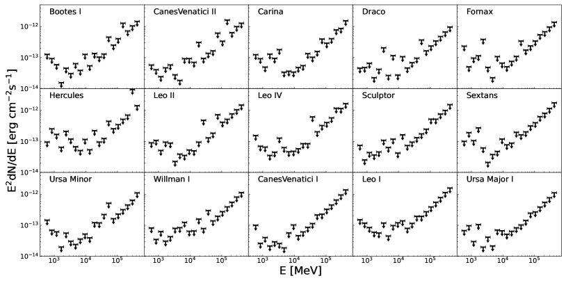
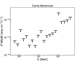
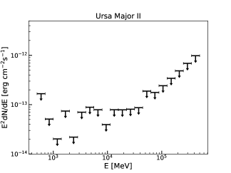
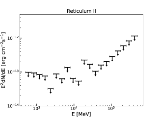
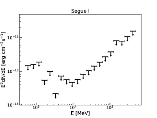
To obtain energy-dependent flux upper limits, we divide the whole energy range of into 20 logarithmically-spaced energy bins. For each energy bin, the background sources are fixed and a power-law spectral model () with =2 Ackermann et al. (2015) is used to model the putative dSph source. We get the upper limits on flux at a confidence level when the log-likelihood () changes by 1.35 Rolke et al. (2005). The energy-dependent flux upper limits for the 4 sources with the biggest J-factors are shown in Fig. 1, while the flux upper limits for other dSphs in our sample are presented in Appendix B.
| Name | TS | |||
|---|---|---|---|---|
| [deg] | [] | [] | ||
| Bootes I | (358.1, 69.6) | 16.54 / 16.84 | 0.00 | |
| CanesVenatici II | (113.6, 82.7) | 17.48 / 17.94 | 2.51 | |
| Carina | (260.1, -22.2) | 17.90 / 18.15 | 0.00 | |
| ComaBerenices | (241.9, 83.6) | 18.56 / 18.85 | 0.00 | |
| Draco | (86.4, 34.7) | 18.87 / 19.00 | 0.00 | |
| Fornax | (237.1, -65.7) | 18.07 / 18.29 | 1.73 | |
| Hercules | (28.7, 36.9) | 16.56 / 17.28 | 4.53 | |
| Leo II | (220.2, 67.2) | 17.41 / 17.49 | 0.00 | |
| Leo IV | (265.4, 56.5) | 16.48 / 16.90 | 0.00 | |
| Sculptor | (287.5, -83.2) | 18.56 / 18.80 | 0.00 | |
| Segue I | (220.5, 50.4) | 19.26 / 19.66 | 2.74 | |
| Sextans | (243.5, 42.3) | 17.77 / 18.04 | 0.00 | |
| UrsaMajor II | (152.5, 37.4) | 19.15 / 19.77 | 0.00 | |
| UrsaMinor | (105.0, 44.8) | 18.96 / 19.47 | 1.20 | |
| Willman I | (158.6, 56.8) | 19.14 / 19.54 | 8.16 | |
| CanesVenatici I | (74.3, 79.8) | 17.15 / 17.46 | 0.00 | |
| Leo I | (226.0, 49.1) | 17.75 / 17.89 | 1.53 | |
| UrsaMajor I | (159.4, 54.4) | 18.11 / 19.11 | 0.00 | |
| Reticulum II | (266.3, -49.7) | 18.50 / 19.06 | 7.36 |
- •
-
•
2 J-factors taken from Sanders et al. (2016), which have accounted for the flattening of the dSphs. The left and right values are for the oblate and prolate cases, respectively.
To improve the sensitivity, we also perform a stacking analysis of our sample. The stacking analysis can give a better sensitivity by merging the observations of multiple sources. We sum the data (i.e. the count cubes in the binned likelihood analysis) of these sources together. The likelihood is evaluated by
| (4) |
where and is the model-predicted and observed counts in each pixel, respectively, and the index runs over all energy and spatial bins. For our stacking analysis, and with index summing over all target sources. The is obtained using the gtmodel command in the Fermitool software, while the is the counts cube obtained using the gtbin command. The model map is related to the DM model parameters and the dSph J-factor, . The DM annihilation flux is implemented in the analysis with a FileFunction spectrum333https://fermi.gsfc.nasa.gov/ssc/data/analysis/scitools/source_models.html#FileFunction (see Sec. IV for the calculation of the expected DM spectrum). Note that the method used here is not the same as the commonly-used combined likelihood analysis Ackermann et al. (2011); Tsai et al. (2013); Ackermann et al. (2014, 2015). The advantage of our method is that it can effectively avoid the loss of sensitivity due to the uncertainty of J-factor. For comparison, we also perform the combined analysis (see Appendix A for details) which gives similar results and the same conclusion.
We use the above method to scan a series of DM masses. Since we are focusing on the i2HDM model that can commonly interpret the W-boson mass anomaly, the GC GeV excess and the antiproton excess, we scan the masses from 45 GeV to 140 GeV for DM annihilation channel . For all dSphs, no significant (i.e. ) signals are found in our analyses. We show our results in Table 1. One reason why our analysis does not give a relatively high TS value (i.e. ) as in previous results Geringer-Sameth et al. (2015); Hooper and Linden (2015); Drlica-Wagner et al. (2015); Albert et al. (2017); Li et al. (2018); Hoof et al. (2020) for the source Reticulum II is that we have added an additional source 0.15∘ away from Reticulum II into the background model. In our previous work we have shown that the excess from the direction of Reticulum II offsets this dSph by and may be not associated with it Li et al. (2021). If not subtracting this excess, we will obtain weaker constraints on the model, but the conclusions would not change. In the stacking analysis, the TS value for the total emission from the dSphs is .
IV Constraints on the cross section of annihilation
Since we do not find any signals from the directions of these dSphs (both individual and stacking analyses), we test whether the i2HDM parameters accounting for the three anomaly/excesses are in tension with the dSph’s null results. We derive the upper limits on the cross section for a series of DM masses of 45-140 GeV. The method described in the Sec. III are used to get the constraints on the cross section. The expected -ray flux from DM annihilation reads
| (5) |
where and are the DM particle mass and the velocity-averaged DM annihilation cross section. The term
| (6) |
is the so-called J-factor, which can be determined through stellar kinematics. The J-factors of our sources are listed in Table 1 which are extracted from Ref. Ackermann et al. (2015); Simon et al. (2015). The is the differential -ray yield per annihilation. For the channel and when the DM mass is , the off-shell annihilation into is considered and we use the spectra the same as those in Zhu et al. (2022), which is simulated with MadGraph5_aMC@NLO Alwall et al. (2014) and PYTHIA8 Sjöstrand et al. (2015). For the DM mass , the DM spectra are obtained from PPP4DMID Cirelli et al. (2011).
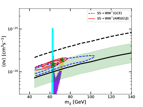
The obtained constraints are shown in Fig. 2. The i2HDM parameters that can simultaneously interpret the W-boson mass anomaly, the GC GeV excess and the GeV antiproton excess are the overlapping parameters of the red and blue contours and the colored points, and are within very small regions around the star symbols. We find that our upper limits (the thick black line) are below the favored parameters, suggesting that the dSph observations seem to be able to exclude such a model.
We would like to give some comments and discussions on this result. Firstly, it should be noted that our results exclude only the parameter space that can simultaneously explain the three anomaly/excesses, but not the whole i2HDM model of accounting for the W-boson mass anomaly. For the i2HDM model with cross section , it can still be used to explain the CDF II W-boson mass. In fact, as is shown in Fig. 2, our limits mainly exclude the parameters related to the GC excess (blue contour) and the GeV antiproton excess (red contour). Such a conclusion is supported by some previous works, which also showed that the best-fit GC excess parameters are not favored by the dSph observations Ackermann et al. (2015); Albert et al. (2017); Hoof et al. (2020); Abdalla et al. (2021).
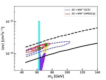
However, the dSph constraints (including our results) are reliant on the accuracy of the J-factor measurements, but actually there are substantial uncertainties in current J-factor measurements. As seen in Liang et al. (2016), for the same data analysis, the use of J-factors provided by different groups can lead to results that differ by a factor of several. Moreover, some studies have revealed that the existing estimations of J-factors are not conservative. For example, Ref. Ichikawa et al. (2017) figures out that considering the contamination of foreground stars may decrease the J-factors by a factor of 3 (thus weakening the dSph constraints by a factor of 3); numerical simulations of galaxy formation that take into account the baryonic effects also point out that the flux of DM annihilation from dSphs may be much lower than that of the Galactic center Grand and White (2021), thus making the null detection in our analysis reasonable even if the GC GeV excess was a true DM signal. Another source of uncertainty that should also be assessed is the flattening of the dSphs. Our benchmark limits (the thick black line in Fig. 2) is derived based on the J-factors that are calculated assuming spherical models of the dSphs. It is argued that the flattening of the galaxies will lead to J-factor values different by tens of percent Sanders et al. (2016) (the J-factors that consider the flattening are also listed in Table I). The shaded band in Fig. 2 illustrates the variation of the limits on due to the flattening, where the upper (bottom) bound assumes that the dSphs are all oblate (prolate). Finally we also do not consider the extension of dSphs in our data analysis, instead treating dSphs as point-like sources. Ref. Di Mauro et al. (2022) has shown that taking into account the extension of dSphs, the limits on DM parameters will be weakened by a factor of . Considering all these factors, the constraints from dSphs are possible to be several times weaker and thus unable to constrain the model (see the dashed line in Fig. 2).
Therefore, it will be crucial to use better observations of dSphs from future observatories (e.g., Vera C. Rubin Observatory LSST Science Collaboration et al. (2009)) to accurately determine the J-factor values. The next generation gamma-ray telescopes with a sensitivity several times better (e.g., VLAST Fan et al. (2022)) is also promising to give a reliable answer to the problem.
V Summary
The new measurement of W-boson mass by the CDF collaboration shows that the mass deviates from the Standard Model prediction with a significance of Aaltonen et al. (2022). This result indicates there may exist new physics beyond the SM (see however the recent W-boson mass measurements by the ATLAS collaboration The ATLAS collaboration (2023); Aaboud et al. (2018), which do not support the results by CDF). Ref. Fan et al. (2022); Zhu et al. (2022) proposed that the inert two Higgs doublet model (i2HDM) can well explain the new W-boson mass. More encouragingly, they found that this model can also explain both the GeV gamma-ray excess in the Galactic center and the GeV antiproton excess with common parameters. The gamma rays and cosmic rays are produced through a annihilation with the lightest stable particle in the i2HDM which can play the role of DM.
In this paper, we have tested the possible common origin of the three anomaly/excesses by analyzing the Fermi-LAT observations of dSphs using the dSph J-factors reported in Refs. Ackermann et al. (2015); Simon et al. (2015). The Milky Way dSphs are an ideal source population to test DM models due to their large J-factors and low gamma-ray background. We do not find any significant signal in both the single-source and the stacking analyses. Based on the null results, we place constraints on the cross section of the self-annihilation of the DM paticle . We find that our constraints seems to be able to exclude, at a 95% confidence level, the favored parameters reported in Ref. Zhu et al. (2022) that can simultaneously interpret the W-boson mass anomaly, the GC excess and the antiproton excess. However, we point out that there exist uncertainties in our exclusion limits and we still cannot reliably claim that the common origin has been excluded. The reason is that the model parameters are only marginally excluded while the exclusion line we obtained relies on the accuracy of the J-factor measurements which however suffers from considerable uncertainties. It is expected that future detectors with higher sensitivity (e.g., VLAST) will be able to solve this problem (either reliably exclude the model or detect a signal).
Acknowledgements.
We thank Yizhong Fan, Ziqing Xia, Zhaohuan Yu and Qiang Yuan for providing us the DM annihilation spectra of channel and for the helpful communications. This work is supported by the National Key Research and Development Program of China (No. 2022YFF0503304) and the Guangxi Science Foundation (grant No. 2019AC20334).References
- Ade et al. (2016) P. A. R. Ade et al. (Planck Collaboration), “Planck 2015 results. XIII. Cosmological parameters,” Astron. Astrophys. 594, A13 (2016), arXiv:1502.01589.
- Jungman et al. (1996) G. Jungman, M. Kamionkowski, and K. Griest, “Supersymmetric dark matter,” Phys. Rept. 267, 195 (1996), arXiv:hep-ph/9506380.
- Bertone et al. (2005) G. Bertone, D. Hooper, and J. Silk, “Particle dark matter: Evidence, candidates and constraints,” Phys. Rept. 405, 279 (2005), arXiv:hep-ph/0404175.
- Hooper and Profumo (2007) D. Hooper and S. Profumo, “Dark matter and collider phenomenology of universal extra dimensions,” Phys. Rept. 453, 29 (2007), arXiv:hep-ph/0701197.
- Feng (2010) J. L. Feng, “Dark Matter Candidates from Particle Physics and Methods of Detection,” Ann. Rev. Astron. Astrophys. 48, 495 (2010), arXiv:1003.0904.
- Evans et al. (2004) N. W. Evans, F. Ferrer, and S. Sarkar, “A travel guide to the dark matter annihilation signal,” Phys. Rev. D 69, 123501 (2004).
- Atwood et al. (2009) W. B. Atwood et al. (Fermi-LAT Collaboration), “The Large Area Telescope on the Fermi Gamma-ray Space Telescope Mission,” Astrophys. J. 697, 1071 (2009), arXiv:0902.1089.
- Charles et al. (2016) E. Charles et al. (Fermi-LAT Collaboration), “Sensitivity Projections for Dark Matter Searches with the Fermi Large Area Telescope,” Phys. Rept. 636, 1 (2016), arXiv:1605.02016.
- Chang et al. (2017) J. Chang et al. (DAMPE Collaboration), “The DArk Matter Particle Explorer mission,” Astropart. Phys. 95, 6 (2017), arXiv:1706.08453.
- Ambrosi et al. (2017) G. Ambrosi et al. (DAMPE Collaboration), “Direct detection of a break in the teraelectronvolt cosmic-ray spectrum of electrons and positrons,” Nature 552, 63 (2017), arXiv:1711.10981.
- Liu et al. (2022) T.-C. Liu, J.-G. Cheng, Y.-F. Liang, and E.-W. Liang, “Search for gamma-ray line signals around the black hole at the galactic center with DAMPE observation,” Sci. China Phys. Mech. Astron. 65, 269512 (2022), arXiv:2203.08078.
- Aaltonen et al. (2022) T. Aaltonen et al. (CDF Collaboration), “High-precision measurement of the boson mass with the CDF II detector,” Science 376, 170 (2022).
- Schael et al. (2013) S. Schael et al. (ALEPH, DELPHI, L3, OPAL, LEP Electroweak Collaboration), “Electroweak Measurements in Electron-Positron Collisions at W-Boson-Pair Energies at LEP,” Phys. Rept. 532, 119 (2013), arXiv:1302.3415.
- Aaboud et al. (2018) M. Aaboud et al. (ATLAS Collaboration), “Measurement of the -boson mass in pp collisions at TeV with the ATLAS detector,” Eur. Phys. J. C 78, 110 (2018), [Erratum: Eur.Phys.J.C 78, 898 (2018)], arXiv:1701.07240.
- Aaij et al. (2022) R. Aaij et al. (LHCb Collaboration), “Measurement of the W boson mass,” JHEP 01, 036 (2022), arXiv:2109.01113.
- Athron et al. (2023) P. Athron, A. Fowlie, C.-T. Lu, L. Wu, Y. Wu, and B. Zhu, “Hadronic uncertainties versus new physics for the W boson mass and Muon g 2 anomalies,” Nature Commun. 14, 659 (2023), arXiv:2204.03996.
- Lu et al. (2022) C.-T. Lu, L. Wu, Y. Wu, and B. Zhu, “Electroweak precision fit and new physics in light of the W boson mass,” Phys. Rev. D 106, 035034 (2022), arXiv:2204.03796.
- Tang et al. (2023) T.-P. Tang, M. Abdughani, L. Feng, Y.-L. S. Tsai, J. Wu, and Y.-Z. Fan, “NMSSM neutralino dark matter for CDF II W-boson mass and muon g 2 and the promising prospect of direct detection,” Sci. China Phys. Mech. Astron. 66, 239512 (2023), arXiv:2204.04356.
- Yuan et al. (2022) G.-W. Yuan, L. Zu, L. Feng, Y.-F. Cai, and Y.-Z. Fan, “Is the W-boson mass enhanced by the axion-like particle, dark photon, or chameleon dark energy?” Sci. China Phys. Mech. Astron. 65, 129512 (2022), arXiv:2204.04183.
- Du et al. (2023) X. K. Du, Z. Li, F. Wang, and Y. K. Zhang, “The muon g2 anomaly in EOGM with adjoint messengers,” Nucl. Phys. B 989, 116151 (2023), arXiv:2204.04286.
- Yang and Zhang (2022) J. M. Yang and Y. Zhang, “Low energy SUSY confronted with new measurements of W-boson mass and muon g-2,” Sci. Bull. 67, 1430 (2022), arXiv:2204.04202.
- Strumia (2022) A. Strumia, “Interpreting electroweak precision data including the W-mass CDF anomaly,” JHEP 08, 248 (2022), arXiv:2204.04191.
- Endo and Mishima (2022) M. Endo and S. Mishima, “New physics interpretation of W-boson mass anomaly,” Phys. Rev. D 106, 115005 (2022), arXiv:2204.05965.
- Han et al. (2022) X.-F. Han, F. Wang, L. Wang, J. M. Yang, and Y. Zhang, “Joint explanation of W-mass and muon g–2 in the 2HDM*,” Chin. Phys. C 46, 103105 (2022), arXiv:2204.06505.
- Ahn et al. (2022) Y. H. Ahn, S. K. Kang, and R. Ramos, “Implications of New CDF-II Boson Mass on Two Higgs Doublet Model,” Phys. Rev. D 106, 055038 (2022), arXiv:2204.06485.
- Zheng et al. (2022) M.-D. Zheng, F.-Z. Chen, and H.-H. Zhang, “The -vertex corrections to W-boson mass in the R-parity violating MSSM,” (2022), arXiv:2204.06541.
- Fileviez Perez et al. (2022) P. Fileviez Perez, H. H. Patel, and A. D. Plascencia, “On the W mass and new Higgs bosons,” Phys. Lett. B 833, 137371 (2022), arXiv:2204.07144.
- Zhang and Feng (2023) K.-Y. Zhang and W.-Z. Feng, “Explaining the W boson mass anomaly and dark matter with a U(1) dark sector*,” Chin. Phys. C 47, 023107 (2023), arXiv:2204.08067.
- Borah et al. (2022) D. Borah, S. Mahapatra, D. Nanda, and N. Sahu, “Type II Dirac seesaw with observable Neff in the light of W-mass anomaly,” Phys. Lett. B 833, 137297 (2022), arXiv:2204.08266.
- Zeng et al. (2023) Y.-P. Zeng, C. Cai, Y.-H. Su, and H.-H. Zhang, “Z boson mixing and the mass of the W boson,” Phys. Rev. D 107, 056004 (2023), arXiv:2204.09487.
- Du et al. (2022) M. Du, Z. Liu, and P. Nath, “CDF W mass anomaly with a Stueckelberg-Higgs portal,” Phys. Lett. B 834, 137454 (2022), arXiv:2204.09024.
- Fan et al. (2022) Y.-Z. Fan, T.-P. Tang, Y.-L. S. Tsai, and L. Wu, “Inert Higgs Dark Matter for CDF II W-Boson Mass and Detection Prospects,” Phys. Rev. Lett. 129, 091802 (2022), arXiv:2204.03693.
- Zhu et al. (2022) C.-R. Zhu, M.-Y. Cui, Z.-Q. Xia, Z.-H. Yu, X. Huang, Q. Yuan, and Y.-Z. Fan, “Explaining the GeV Antiproton Excess, GeV -Ray Excess, and W-Boson Mass Anomaly in an Inert Two Higgs Doublet Model,” Phys. Rev. Lett. 129, 231101 (2022), arXiv:2204.03767.
- Hooper and Goodenough (2011) D. Hooper and L. Goodenough, “Dark Matter Annihilation in The Galactic Center As Seen by the Fermi Gamma Ray Space Telescope,” Phys. Lett. B 697, 412 (2011), arXiv:1010.2752.
- Gordon and Macias (2013) C. Gordon and O. Macias, “Dark Matter and Pulsar Model Constraints from Galactic Center Fermi-LAT Gamma Ray Observations,” Phys. Rev. D 88, 083521 (2013), [Erratum: Phys. Rev.D89,no.4,049901(2014)], arXiv:1306.5725.
- Hooper and Slatyer (2013) D. Hooper and T. R. Slatyer, “Two Emission Mechanisms in the Fermi Bubbles: A Possible Signal of Annihilating Dark Matter,” Phys. Dark Univ. 2, 118 (2013), arXiv:1302.6589.
- Daylan et al. (2016) T. Daylan, D. P. Finkbeiner, D. Hooper, T. Linden, S. K. N. Portillo, N. L. Rodd, and T. R. Slatyer, “The characterization of the gamma-ray signal from the central Milky Way: A case for annihilating dark matter,” Physics of the Dark Universe 12, 1 (2016), arXiv:1402.6703.
- Zhou et al. (2015) B. Zhou, Y.-F. Liang, X. Huang, X. Li, Y.-Z. Fan, L. Feng, and J. Chang, “GeV excess in the Milky Way: The role of diffuse galactic gamma-ray emission templates,” Phys. Rev. D 91, 123010 (2015), arXiv:1406.6948.
- Calore et al. (2015) F. Calore, I. Cholis, and C. Weniger, “Background model systematics for the Fermi GeV excess,” JCAP 1503, 038 (2015), arXiv:1409.0042.
- Ackermann et al. (2017) M. Ackermann et al., “The Fermi Galactic Center GeV Excess and Implications for Dark Matter,” Astrophys. J. 840, 43 (2017), arXiv:1704.03910.
- Cui et al. (2017) M.-Y. Cui, Q. Yuan, Y.-L. S. Tsai, and Y.-Z. Fan, “Possible Dark Matter Annihilation Signal in the AMS-02 Antiproton Data,” Physical Review Letters 118, 191101 (2017), arXiv:1610.03840.
- Cuoco et al. (2017) A. Cuoco, M. Krämer, and M. Korsmeier, “Novel Dark Matter Constraints from Antiprotons in Light of AMS-02,” Physical Review Letters 118, 191102 (2017), arXiv:1610.03071.
- Lake (1990) G. Lake, “Detectability of gamma-rays from clumps of dark matter,” Nature 346, 39 (1990).
- Baltz and Wai (2004) E. A. Baltz and L. Wai, “Diffuse inverse Compton and synchrotron emission from dark matter annihilations in galactic satellites,” Phys. Rev. D 70, 023512 (2004), arXiv:astro-ph/0403528.
- Strigari (2013) L. E. Strigari, “Galactic Searches for Dark Matter,” Phys. Rept. 531, 1 (2013), arXiv:1211.7090.
- Ackermann et al. (2011) M. Ackermann et al., “Constraining Dark Matter Models from a Combined Analysis of Milky Way Satellites with the Fermi Large Area Telescope,” Physical Review Letters 107, 241302 (2011), arXiv:1108.3546.
- Geringer-Sameth and Koushiappas (2011) A. Geringer-Sameth and S. M. Koushiappas, “Exclusion of canonical WIMPs by the joint analysis of Milky Way dwarfs with Fermi,” Phys. Rev. Lett. 107, 241303 (2011), arXiv:1108.2914.
- Cholis and Salucci (2012) I. Cholis and P. Salucci, “Extracting limits on dark matter annihilation from gamma ray observations towards dwarf spheroidal galaxies,” Phys. Rev. D 86, 023528 (2012), arXiv:1203.2954.
- Tsai et al. (2013) Y.-L. S. Tsai, Q. Yuan, and X. Huang, “A generic method to constrain the dark matter model parameters from Fermi observations of dwarf spheroids,” JCAP 1303, 018 (2013), arXiv:1212.3990.
- Ackermann et al. (2014) M. Ackermann et al., “Dark matter constraints from observations of 25 Milky Way satellite galaxies with the Fermi Large Area Telescope,” Phys. Rev. D 89, 042001 (2014), arXiv:1310.0828.
- Zhao et al. (2016) Y. Zhao, X.-J. Bi, H.-Y. Jia, P.-F. Yin, and F.-R. Zhu, “Constraint on the velocity dependent dark matter annihilation cross section from Fermi-LAT observations of dwarf galaxies,” Phys. Rev. D93, 083513 (2016), arXiv:1601.02181.
- Geringer-Sameth et al. (2015) A. Geringer-Sameth, S. M. Koushiappas, and M. G. Walker, “Comprehensive search for dark matter annihilation in dwarf galaxies,” Phys. Rev. D 91, 083535 (2015), arXiv:1410.2242.
- Ackermann et al. (2015) M. Ackermann et al., “Searching for Dark Matter Annihilation from Milky Way Dwarf Spheroidal Galaxies with Six Years of Fermi Large Area Telescope Data,” Physical Review Letters 115, 231301 (2015), arXiv:1503.02641.
- Hoof et al. (2020) S. Hoof, A. Geringer-Sameth, and R. Trotta, “A global analysis of dark matter signals from 27 dwarf spheroidal galaxies using 11 years of Fermi-LAT observations,” J. Cosmol. Astropart. Phys. 2020, 012 (2020), arXiv:1812.06986.
- Deshpande and Ma (1978) N. G. Deshpande and E. Ma, “Pattern of Symmetry Breaking with Two Higgs Doublets,” Phys. Rev. D 18, 2574 (1978).
- Ma (2006) E. Ma, “Verifiable radiative seesaw mechanism of neutrino mass and dark matter,” Phys. Rev. D 73, 077301 (2006), arXiv:hep-ph/0601225.
- Barbieri et al. (2006) R. Barbieri, L. J. Hall, and V. S. Rychkov, “Improved naturalness with a heavy Higgs: An Alternative road to LHC physics,” Phys. Rev. D 74, 015007 (2006), arXiv:hep-ph/0603188.
- Lopez Honorez et al. (2007) L. Lopez Honorez, E. Nezri, J. F. Oliver, and M. H. G. Tytgat, “The Inert Doublet Model: An Archetype for Dark Matter,” JCAP 02, 028 (2007), arXiv:hep-ph/0612275.
- Peskin and Takeuchi (1992) M. E. Peskin and T. Takeuchi, “Estimation of oblique electroweak corrections,” Phys. Rev. D 46, 381 (1992).
- Eriksson et al. (2010) D. Eriksson, J. Rathsman, and O. Stal, “2HDMC: Two-Higgs-Doublet Model Calculator Physics and Manual,” Comput. Phys. Commun. 181, 189 (2010), arXiv:0902.0851.
- Arhrib et al. (2014) A. Arhrib, Y.-L. S. Tsai, Q. Yuan, and T.-C. Yuan, “An Updated Analysis of Inert Higgs Doublet Model in light of the Recent Results from LUX, PLANCK, AMS-02 and LHC,” JCAP 06, 030 (2014), arXiv:1310.0358.
- Tsai et al. (2020) Y.-L. S. Tsai, V. Q. Tran, and C.-T. Lu, “Confronting dark matter co-annihilation of Inert two Higgs Doublet Model with a compressed mass spectrum,” JHEP 06, 033 (2020), arXiv:1912.08875.
- Abdollahi et al. (2020) S. Abdollahi et al., “Fermi Large Area Telescope Fourth Source Catalog,” Astrophys. J. Suppl. 247, 33 (2020), arXiv:1902.10045.
- Mattox et al. (1996) J. R. Mattox et al., “The Likelihood Analysis of EGRET Data,” Astrophys. J. 461, 396 (1996).
- Rolke et al. (2005) W. A. Rolke, A. M. López, and J. Conrad, “Limits and confidence intervals in the presence of nuisance parameters,” Nuclear Instruments and Methods in Physics Research Section A: Accelerators, Spectrometers, Detectors and Associated Equipment 551, 493 (2005).
- Simon et al. (2015) J. D. Simon et al. (DES Collaboration), “Stellar Kinematics and Metallicities in the Ultra-Faint Dwarf Galaxy Reticulum II,” Astrophys. J. 808, 95 (2015), arXiv:1504.02889.
- Sanders et al. (2016) J. L. Sanders, N. W. Evans, A. Geringer-Sameth, and W. Dehnen, “Indirect Dark Matter Detection for Flattened Dwarf Galaxies,” Phys. Rev. D 94, 063521 (2016), arXiv:1604.05493.
- Geringer-Sameth et al. (2015) A. Geringer-Sameth, M. G. Walker, S. M. Koushiappas, S. E. Koposov, V. Belokurov, G. Torrealba, and N. W. Evans, “Indication of Gamma-ray Emission from the Newly Discovered Dwarf Galaxy Reticulum II,” Phys. Rev. Lett. 115, 081101 (2015), arXiv:1503.02320.
- Hooper and Linden (2015) D. Hooper and T. Linden, “On The Gamma-Ray Emission From Reticulum II and Other Dwarf Galaxies,” JCAP 1509, 016 (2015), arXiv:1503.06209.
- Drlica-Wagner et al. (2015) A. Drlica-Wagner et al. (DES, Fermi-LAT Collaboration), “Search for Gamma-Ray Emission from DES Dwarf Spheroidal Galaxy Candidates with Fermi-LAT Data,” Astrophys. J. 809, L4 (2015), arXiv:1503.02632.
- Albert et al. (2017) A. Albert et al. (Fermi-LAT, DES Collaboration), “Searching for Dark Matter Annihilation in Recently Discovered Milky Way Satellites with Fermi-LAT,” Astrophys. J. 834, 110 (2017), arXiv:1611.03184.
- Li et al. (2018) S. Li et al., “Search for gamma-ray emission from the nearby dwarf spheroidal galaxies with 9 years of Fermi-LAT data,” Phys. Rev. D 97, 122001 (2018), arXiv:1805.06612.
- Li et al. (2021) S. Li, Y.-F. Liang, and Y.-Z. Fan, “Search for gamma-ray emission from the 12 nearby dwarf spheroidal galaxies with 12 years of Fermi-LAT data,” Phys. Rev. D 104, 083037 (2021), arXiv:2110.01157.
- Alwall et al. (2014) J. Alwall, R. Frederix, S. Frixione, V. Hirschi, F. Maltoni, O. Mattelaer, H. S. Shao, T. Stelzer, P. Torrielli, and M. Zaro, “The automated computation of tree-level and next-to-leading order differential cross sections, and their matching to parton shower simulations,” Journal of High Energy Physics 2014, 79 (2014), arXiv:1405.0301.
- Sjöstrand et al. (2015) T. Sjöstrand, S. Ask, J. R. Christiansen, R. Corke, N. Desai, P. Ilten, S. Mrenna, S. Prestel, C. O. Rasmussen, and P. Z. Skands, “An introduction to PYTHIA 8.2,” Computer Physics Communications 191, 159 (2015), arXiv:1410.3012.
- Cirelli et al. (2011) M. Cirelli, G. Corcella, A. Hektor, G. Hutsi, M. Kadastik, P. Panci, M. Raidal, F. Sala, and A. Strumia, “PPPC 4 DM ID: A Poor Particle Physicist Cookbook for Dark Matter Indirect Detection,” JCAP 1103, 051 (2011), [Erratum: JCAP1210,E01(2012)], arXiv:1012.4515.
- Abdalla et al. (2021) H. Abdalla et al. (Hess, HAWC, VERITAS, MAGIC, H.E.S.S., Fermi-LAT Collaboration), “Combined dark matter searches towards dwarf spheroidal galaxies with Fermi-LAT, HAWC, H.E.S.S., MAGIC, and VERITAS,” PoS ICRC2021, 528 (2021), arXiv:2108.13646.
- Liang et al. (2016) Y.-F. Liang, Z.-Q. Xia, Z.-Q. Shen, X. Li, W. Jiang, Q. Yuan, Y.-Z. Fan, L. Feng, E.-W. Liang, and J. Chang, “Search for gamma-ray line features from Milky Way satellites with Fermi LAT Pass 8 data,” Phys. Rev. D94, 103502 (2016), arXiv:1608.07184.
- Ichikawa et al. (2017) K. Ichikawa, M. N. Ishigaki, S. Matsumoto, M. Ibe, H. Sugai, K. Hayashi, and S.-i. Horigome, “Foreground effect on the -factor estimation of classical dwarf spheroidal galaxies,” Mon. Not. Roy. Astron. Soc. 468, 2884 (2017), arXiv:1608.01749.
- Grand and White (2021) R. J. J. Grand and S. D. M. White, “Baryonic effects on the detectability of annihilation radiation from dark matter subhaloes around the Milky Way,” Mon. Not. R. Astron. Soc. 501, 3558 (2021), arXiv:2012.07846.
- Di Mauro et al. (2022) M. Di Mauro, M. Stref, and F. Calore, “Investigating the effect of Milky Way dwarf spheroidal galaxies extension on dark matter searches with Fermi-LAT data,” Phys. Rev. D 106, 123032 (2022), arXiv:2212.06850.
- LSST Science Collaboration et al. (2009) LSST Science Collaboration et al., “LSST Science Book, Version 2.0,” arXiv e-prints , arXiv:0912.0201 (2009), arXiv:0912.0201.
- Fan et al. (2022) Y. Z. Fan et al., “Very Large Area Gamma-ray Space Telescope (VLAST),” Acta Astronomica Sinica 63, 27 (2022).
- The ATLAS collaboration (2023) The ATLAS collaboration (ATLAS Collaboration), “Improved W boson Mass Measurement using 7 TeV Proton-Proton Collisions with the ATLAS Detector,” ATLAS conference note (2023).
Appendix A Combined likelihood analysis
In order to verify the stacking analysis employed in our main text (the data and model are respectively summed over all sources before calculating the likelihood), here we also use the combined likelihood analysis (the likelihoods are calculated source by source and then summed together to obtain a total likelihood), which has been widely used in previous studies Ackermann et al. (2011); Tsai et al. (2013); Ackermann et al. (2014, 2015), to derive the corresponding results for comparison. We divide the data in the energy range of 500 MeV-500 GeV into 20 logarithmically-spaced energy bins. For each energy bin we vary the scale parameter of the dSph component and derive the relation between the likelihood and the target flux within the th bin , (namely the likelihood profile). The total likelihood considering all energy bins for the DM model with parameters and is given by:
| (7) |
To combine all sources in the sample, the combined likelihood is
| (8) |
with the Eq. (7) and for the th source. In the combined analysis, we also consider the statistical uncertainty in the J-factors, which is incorporated into the likelihood through the term
| (9) |
where and are the measured J-factor and its uncertainty for the source . For a given , the upper limit on at a 95% confidence level is derived by requiring to change by 1.35. We show the constraints based on the combined analysis in Fig. 3.
Appendix B Bin-by-bin flux upper limits for other sources