TTK-22-14
Dark Matter constraints from Planck observations
of the Galactic polarized synchrotron emission
Abstract
Dark Matter (DM) annihilation in our Galaxy may produce a linearly polarized synchrotron signal. We use, for the first time, synchrotron polarization to constrain the DM annihilation cross section by comparing theoretical predictions with the latest polarization maps obtained by the Planck satellite collaboration. We find that synchrotron polarization is typically more constraining than synchrotron intensity by about one order of magnitude, independently of uncertainties in the modeling of electron and positron propagation, or of the Galactic magnetic field. Our bounds compete with Cosmic Microwave Background limits in the case of leptophilic DM.
Introduction. High-energetic cosmic-ray (CR) electrons and positrons ( in what follows) can be either accelerated in primary sources such as supernova remnants and pulsar wind nebulae, or produced by spallation of hadronic CRs. Besides, CR might also be produced by the annihilation or decay of dark matter (DM) particles in the Galactic DM halo. Relativistic then gyrate and propagate in the interstellar Galactic magnetic field (GMF), and produce secondary emissions such as radio and microwave emission through the synchrotron process. The synchrotron signal of DM origin has been extensively investigated in the past using many radio and microwave surveys, such as WMAP and Planck, finding constraints which are complementary to other probes both for the Galactic halo Blasi et al. (2003); Hooper (2008); Borriello et al. (2009); Regis and Ullio (2009); Delahaye et al. (2012); Fornengo et al. (2012); Mambrini et al. (2012); Bringmann et al. (2014); Egorov et al. (2016); Cirelli and Taoso (2016) and extragalactic targets Tasitsiomi et al. (2004); Colafrancesco et al. (2006); Siffert et al. (2010); Fornengo et al. (2011); Carlson et al. (2013); Regis et al. (2014); Hooper et al. (2012); Fornengo et al. (2014). Previous DM searches focused on the synchrotron total intensity, i.e., the Stokes parameter . However, synchrotron emission of relativistic is partially linearly polarized, and a signal in polarization amplitude (i.e., Stokes ) is thus expected. We here exploit for the first time the Planck polarization maps in order to constrain Galactic DM signals. Polarization data have also been used together with total intensity data to study Galactic synchrotron emission and constrain CR propagation and large scale GMF models in absence of DM annihilation, see e.g. Jaffe et al. (2010); Sun et al. (2008); Strong et al. (2011); Bringmann et al. (2012); Jansson and Farrar (2012a, b); Di Bernardo et al. (2013); Mertsch and Sarkar (2013); Orlando and Strong (2013); Planck Collaboration (2016); Orlando (2018); Jew and Grumitt (2020).
The total intensity and the polarization properties of the DM synchrotron emission depend on the strength and orientation of the GMF, as well as on the spatial and energetic distribution of CR produced by DM. As we shall detail in what follows, the synchrotron intensity and polarization signals are complementary, since they are controlled by different properties of the GMF. We thus expect them to be affected by different systematic uncertainties.
Microwave maps. The Planck instrument measures both the intensity and polarization of the microwave and sub-millimeter sky, in terms of the Stokes components I (intensity) and Q, U (polarization). The polarization amplitude is defined as . In particular, Planck has so far provided the deepest and highest-resolution view of the microwave and sub-millimeter sky by mapping anisotropies in the cosmic microwave background (CMB) radiation. This made it possible to put strong constraints on the standard cosmological model and its possible variations Aghanim et al. (2020a).
The Planck sky maps contain contributions from the CMB as well as many other astrophysical components ranging from compact Galactic and extragalactic sources to diffuse backgrounds as synchrotron and free-free emission in our Galaxy, see e.g. Fig.4 in Ref. Aghanim et al. (2020a). Here we are interested in constraining a possible diffuse signal coming from DM annihilation in our Galaxy which, depending on the DM properties, may contribute significantly to the diffuse background. Since the CMB contribution is well-measured, we consider CMB-subtracted maps. We refrain from modeling and subtracting any other contribution from the diffuse backgrounds, such as the Galactic synchrotron emission. We thus derive conservative DM constraints requiring that the DM signal does not exceed the observed emission, once the CMB contribution has been subtracted.


We use data products corresponding to the third release by the Planck collaboration (PR3) for the low frequency instruments (LFI) at and GHz. Regarding the polarization emission, the PR3 release supersedes all previous releases thanks to significantly lower contamination from systematic errors Akrami et al. (2020). CMB-subtracted maps can be obtained using multi-frequency information. We use the maps processed with the NILC method Akrami et al. (2020), which still contain all the diffuse backgrounds.
They can be downloaded from the Planck legacy archive 111http://pla.esac.esa.int/pla/#maps, files named LFI_ CompMap_Foregrounds-nilc-0XX_R3.00.fits, where XX stands for the frequency channel of 30,44,70 GHz. with a resolution of Nside=1024 222The total number of pixels in the map is related to NSide as = 12 Nside2. in the HEALPix pixelization scheme Górski et al. (2005). This corresponds to a mean spacing between adjacent pixels of about degrees. For each frequency, the downloaded files contain three maps, one for each of the three Stokes parameters . These maps contain the observed blackbody differential brightness temperature 333The relation between the brightness temperature and the flux is recalled in Eq. (2), see also Eq. (S3). in units of , which is connected to the Rayleigh-Jeans differential brightness temperature in by a conversion formula that also accounts for color and leakage corrections based on instrument bandpass, see Ref. Planck Collaboration (2016) for more details.
Before comparing the DM predicted map with observations, we need to build the experimental map and its error map from the available and maps. This is achieved with the following steps:
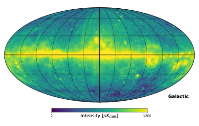
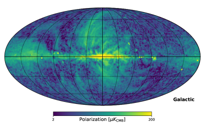
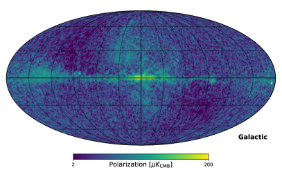
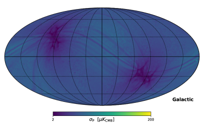
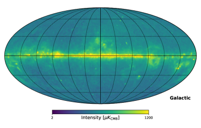
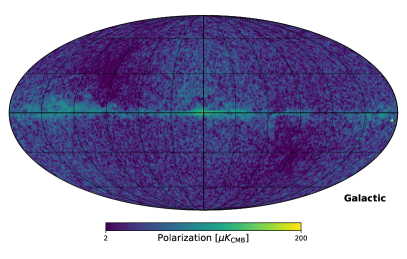
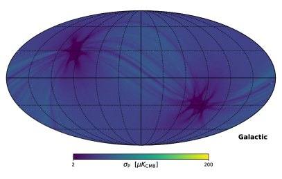
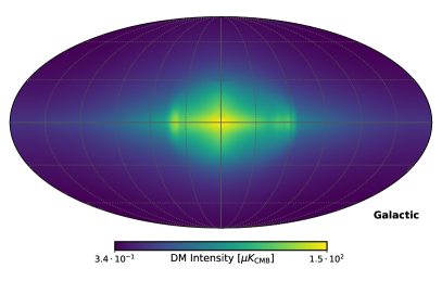
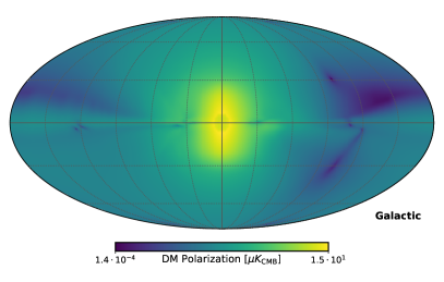
(i) Smoothing. We first smooth the CMB-subtracted maps with a Gaussian beam of degree FWHM, in order to increase the signal-to-noise ratio and reduce systematic effects caused by beam asymmetries. We then create a polarization amplitude map defined as , keeping the original NSide resolution of the maps. The resulting and full-sky maps at GHz are shown in the upper panels of Fig. 1. We provide the full-sky maps at GHz in the supplemental material sup .
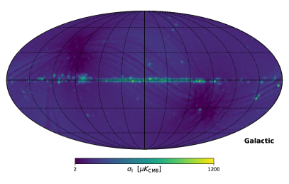
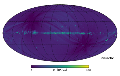
(ii) Error estimation. For the purpose of obtaining robust DM constraints, we need to build error maps from the maps themselves. We estimate the error at each pixel as the variance of all neighboring pixels up to 0.5 degrees, while sticking to the native NSide resolution. This provides an estimate of the noise except in the vicinity of point sources 444In the vicinity of sharp features, like point sources, our method is expected to be biased and to return an error estimate larger than the true one. Nonetheless, this does not affect the final results since pixels with a large error will not contribute to constrain DM.. The error map for is derived from the error maps using error propagation. The resulting sky maps for () for GHz are illustrated in the left (right) lower panel of Fig. 1. One can see by eye that error maps follow the scanning pattern of Planck: the error is smaller where the instrument observes longer, and vice versa.
(iii) Degrading. If needed, the above maps are degraded to a larger pixel resolution. While this is straightforward for the maps, for the error maps one needs to take into account that the error scales with the pixel size. Going from NSide 1024 to a generic lower resolution , we have .
Synchrotron from Galactic dark matter. We consider WIMPs as benchmark DM candidates Roszkowski et al. (2018), and we concentrate on the annihilation signal. However, we stress that the approach presented here could be extended to any search for DM or other exotic particles if they inject in the interstellar medium through annihilation and/or decay processes.
The source term for produced from (Majorana fermions) WIMP annihilations in the Milky Way DM halo reads:
| (1) |
where is the DM mass, is the DM density profile in the Galaxy (assumed to be spherically symmetric), runs over the considered DM annihilation channels, is the velocity averaged cross section, and is the energy spectrum per annihilation for each annihilation channel .
The DM radial distribution in the Galaxy at distance from the halo center can be effectively described by the Navarro-Frenk-White (NFW) and generalized NFW density profile Navarro et al. (1996, 2010), where we fix the scale radius to kpc and enforce the local DM density at the solar position to be GeV/cm3 de Salas and Widmark (2021). To estimate the uncertainties related to the DM radial distribution, particularly relevant for the innermost part, we also consider two additional cases sup . To avoid numerical divergences at the profiles are truncated as detailed in Ref. Egorov et al. (2016). Contributions connected to the presence of DM substructures on top of the main, smooth halo could boost the total DM annihilation rate, and are conservatively not considered here Ando et al. (2019); Ishiyama and Ando (2020).
We consider standard WIMPs with masses between GeV and TeV annihilating into three representative channels: two leptonic channels, and , expected to produce more in their final states, and one hadronic channel , producing a much softer spectrum. The reference thermally averaged annihilation cross section is cm3s-1. The energy spectrum for each channel is taken from the PPPC4DMID library Cirelli et al. (2011) and includes electroweak corrections Ciafaloni et al. (2011).
Cosmic-ray propagation and maps. The propagation of in the interstellar medium can be described through a transport equation which can be solved semi-analytically Maurin (2020) or numerically by different means Hanasz et al. (2021). We here use GALPROP version v54r2766 555publicy available at https://gitlab.mpcdf.mpg.de/aws/galprop as adapted in Ref. Egorov et al. (2016) 666publicy available at https://github.com/a-e-egorov/GALPROP_DM to numerically solve the transport equation and predict the all-sky synchrotron signal maps from DM annihilations. In particular, the computation of the total synchrotron intensity and polarization amplitude is based on the GALPROP developments described in Refs. Strong et al. (2011); Orlando and Strong (2013), and includes free-free absorption, which is however expected to be subdominant at Planck frequencies. GALPROP can solve the transport equation both in two and three spatial dimensions. Since the GMFs we consider are intrinsically 3D, the 3D implementation has to be used to obtain correct predictions. We employ a spatial resolution of pc in each spatial dimension.
To gauge the uncertainties related to propagation we consider three propagation models taken from the literature sup . We employ as a benchmark the plain diffusion model without convection and reacceleration (named PDDE). Refs. Orlando (2018, 2019) found this model to be in agreement with cosmic-ray, synchrotron and gamma-ray data using a similar GALPROP setup. We test also a model with diffusive reacceleration from the same Refs. Orlando (2018, 2019) (named DRE), and a model with convection (named BASE) from the recent Ref. Korsmeier and Cuoco (2021).
We note that GALPROP produces synchrotron maps in units of energyflux, i.e., in units of erg cm-2/s/Hz/sr, where is the frequency and are galactic coordinates. We convert this in brightness temperature as:
| (2) |
which is the temperature that a body with a Rayleigh Jeans (RJ) spectrum would need in order to emit the same intensity at a given frequency . This defines the RJ brightness temperature in units of Kelvins ().
Magnetic field models. The main systematic uncertainty of the present work is anticipated to be associated to the modeling of the GMF, which is still poorly constrained Jaffe (2019). The magnetic field of our Galaxy is know to have at least two components: a large-scale, regular field and an isotropic turbulent, random one. The need for an additional component, called ’ordered random’ Jaffe et al. (2010) or ’striated’ Jansson and Farrar (2012a) has been also recently investigated. This new component corresponds to a large scale ordering of the field, and its intensity is expected to be stronger in the regions between the optical spiral arms. For a comprehensive review on the available tracers, a detailed recap of some current models and their outstanding issues we refer the reader to Ref. Jaffe (2019) (and references therein). We thus rely on past studies which fitted the most updated GMF models to multiwavelength data. To bracket the uncertainties associated to GMF modeling, we consider the following three benchmarks: The Sun+10 model proposed in Refs. Sun et al. (2008); Sun and Reich (2010), the model proposed in Ref. Pshirkov et al. (2011) (Psh+11), and the more sophisticated model presented by Jansson & Farrar for the regular Jansson and Farrar (2012a) and random Jansson and Farrar (2012b) magnetic fields (JF12) sup .
These models differ both for the regular and the random MF component. A crucial observation is the fact that intensity and polarization have a different dependence on the MF. While intensity depends on the total MF (random+ordered), polarization only depends on the regular component. This makes the two probes highly complementary.

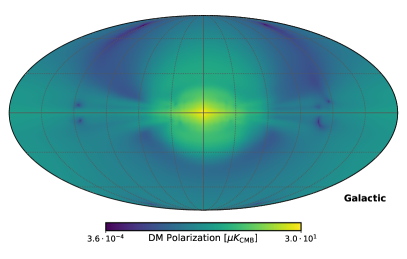
Dark matter signal and constraints. To illustrate the morphology of the polarization DM signals, we show in Fig. 2 the polarization amplitude at GHz for one GMF model (Psh+11). The map is computed for a DM particle of GeV annihilating into pairs with cm3s-1, using the PDDE propagation and for NSide=128. The polarization amplitude of the DM signal is, as expected, peaked at the Galactic center and extends away from the plane following the morphology of the regular magnetic field in the Milky Way disk and halo from Psh+11.
We have validated our results comparing the synchrotron DM maps and spectra with previous works Egorov et al. (2016); Cirelli and Taoso (2016), finding similar results when computing the DM signal within the same setup, when possible. We refer to sup for more examples of the intensity and polarization DM signal maps.
In the following we use Planck LFI maps at GHz as reference, while we show results using higher frequencies maps in sup . For each simulated DM map, i.e., for each DM mass and annihilation channel, we compute an upper bound on the DM annihilation cross section by requiring that the DM intensity or polarization signal at a given frequency does not exceed the observed Planck signal plus the error estimated before, in this way producing limits at the 68% C.L. We enforce this requirement in each pixel at deg, and we provide the upper limit corresponding to the most constraining pixel.
As a preliminary step, we study the effect of pixel size sup . With a small pixel we are sensitive to the detailed morphology of the signal, but the noise per pixel is large, while with a large pixel we have a smaller noise but we lose the details of the morphology. We find that the constraints are optimized for a choice of an NSide=128, that we adopt in the following sup .
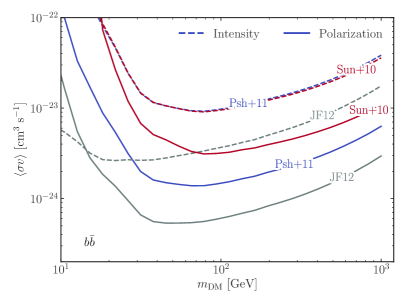
Our results for the upper limits obtained using Planck intensity and polarization data are illustrated in Fig. 3 (left) for different GMF models and for the channel and PDDE propagation setup. At fixed GMF model, we find that the polarization maps are more constraining than the intensity maps by almost one order of magnitude for DM masses larger than 20 GeV. The Sun+10 and Psh+11 models use the same parametrizations and intensity values for the random field, and thus the intensity constraints are very similar. The random field of the JF12 model has instead a more complicated morphology and a larger strength, which translates into stronger limits by a factor of two. The different morphology and strength for the ordered GMF translate into an uncertainty of about one order of magnitude in the upper limits obtained with the polarization data. The JF12 model is in this case associated to the most stringent upper limits given the non-zero striated component included. We recall that the strength of the GMF is highly degenerate with the normalization of the CR density in the Galaxy, and a consistent assessment of the parameters of the GMFs should contextually fit also the CR injection and propagation parameters. We leave this assessment to future work, in which potentially stronger constraints can be derived by modeling and subtracting the astrophysical Galactic synchrotron emission within the same framework.
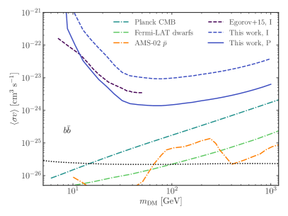
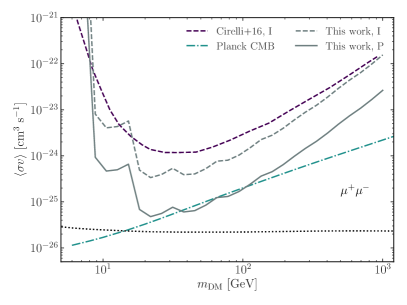
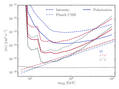
The upper limits corresponding to the three annihilation channels are illustrated in Fig. 3 (right), for a fixed choice of Psh+11 GMF and PDDE propagation setup. The limits reach approximately the same value at about GeV, where the synchrotron emission spectrum from DM annihilations at GHz has similar values for all channels. For all channels, the synchrotron polarization data provide constraints at least a factor of five better than the intensity. For different MF (left panel) this is valid for GeV. At tens of GeV and for annihilations, we exclude larger than about cm3s-1. This is compared to the thermal relic cross section Steigman et al. (2012) shown as a dotted line. For the channel our upper limits using Planck polarization are competitive with Planck CMB constraints Aghanim et al. (2020b) (dot-dashed lines) between about 50 GeV and 100 GeV. We interpret the stronger DM constraints from polarization as coming from two effects. First, the astrophysical backgrounds are lower in polarization rather than in the intensity sup . Secondly, the intensity and polarization maps have significantly different morphologies. In particular, as can be seen in Fig. 1 the polarization map presents filaments, or arms, extending many degrees in the sky. This leaves inter-arms regions with very low background very close to the Galactic center, where the DM signal peaks. Instead, the background for the intensity has a more uniform structure towards the inner Galaxy.
While these limits on WIMPs are overall weaker than some other constraints available in the literature Albert et al. (2017); Leane et al. (2018); Calore et al. (2018); Regis et al. (2021); Cuoco et al. (2017); Kahlhoefer et al. (2021); Calore et al. (2022), the conservative analysis presented in this letter is the first step towards a more detailed assessment of the constraining power of polarization data when also the astrophysical background will be included.
Further systematic uncertainties related to the choice of the propagation setup or the DM radial profile are discussed in sup .
Conclusions. This paper presents a new method to constrain DM properties using for the first time as observable the map of CMB foreground polarization. We have derived new, conservative (i.e., removing only the CMB) DM constraints using Planck synchrotron microwave polarization sky maps. We obtain competitive bounds on the WIMP annihilation cross-section, while we find that polarization maps provide DM limits up to one order of magnitude stronger than the ones coming from intensity maps. Our method could be generalized to other types of particles with electromagnetic annihilation or decay products. The bounds could be straightened by a proper removal of astrophysical foregrounds on top of the CMB background, by a more accurate modeling of the GMF and of the DM density profile, and finally by more sensitive full-sky observations of the polarized millimeter sky (which should be delivered by the LiteBird satellite Hazumi et al. (2020)).
Acknowledgements.
Acknowledgments. We thank Michael Krämer for insightful discussion in the initial stages of this work and GALPROP developers for useful conversation. We also thank Fabio Finelli and Andrea Zacchei for providing further insight on the Planck LFI maps. The work of A.C. is supported by: “Departments of Excellence 2018-2022” grant awarded by the Italian Ministry of Education, University and Research (MIUR) L. 232/2016; Research grant “The Dark Universe: A Synergic Multimessenger Approach” No. 2017X7X85K, PRIN 2017, funded by MIUR; Research grant TAsP (Theoretical Astroparticle Physics) funded by INFN. Simulations were performed with computing resources granted by RWTH Aachen University.References
- Blasi et al. (2003) P. Blasi, A. V. Olinto, and C. Tyler, Astropart. Phys. 18, 649 (2003), arXiv:astro-ph/0202049 .
- Hooper (2008) D. Hooper, Phys. Rev. D 77, 123523 (2008), arXiv:0801.4378 [hep-ph] .
- Borriello et al. (2009) E. Borriello, A. Cuoco, and G. Miele, Phys. Rev. D79, 023518 (2009), arXiv:0809.2990 [astro-ph] .
- Regis and Ullio (2009) M. Regis and P. Ullio, Phys. Rev. D 80, 043525 (2009), arXiv:0904.4645 [astro-ph.GA] .
- Delahaye et al. (2012) T. Delahaye, C. Boehm, and J. Silk, Mon. Not. Roy. Astron. Soc. 422, L16 (2012), arXiv:1105.4689 [astro-ph.GA] .
- Fornengo et al. (2012) N. Fornengo, R. A. Lineros, M. Regis, and M. Taoso, JCAP 2012, 005 (2012), arXiv:1110.4337 [astro-ph.GA] .
- Mambrini et al. (2012) Y. Mambrini, M. H. G. Tytgat, G. Zaharijas, and B. Zaldivar, JCAP 11, 038 (2012), arXiv:1206.2352 [hep-ph] .
- Bringmann et al. (2014) T. Bringmann, M. Vollmann, and C. Weniger, Phys. Rev. D 90, 123001 (2014), arXiv:1406.6027 [astro-ph.HE] .
- Egorov et al. (2016) A. E. Egorov, J. M. Gaskins, E. Pierpaoli, and D. Pietrobon, JCAP 03, 060 (2016), arXiv:1509.05135 [astro-ph.CO] .
- Cirelli and Taoso (2016) M. Cirelli and M. Taoso, JCAP 1607, 041 (2016), arXiv:1604.06267 [hep-ph] .
- Tasitsiomi et al. (2004) A. Tasitsiomi, J. M. Siegal-Gaskins, and A. V. Olinto, Astropart. Phys. 21, 637 (2004), arXiv:astro-ph/0307375 .
- Colafrancesco et al. (2006) S. Colafrancesco, S. Profumo, and P. Ullio, Astron. Astrophys. 455, 21 (2006), arXiv:astro-ph/0507575 .
- Siffert et al. (2010) B. B. Siffert, A. Limone, E. Borriello, G. Longo, and G. Miele, Monthly Notices of the Royal Astronomical Society 410, 2463–2471 (2010).
- Fornengo et al. (2011) N. Fornengo, R. Lineros, M. Regis, and M. Taoso, Phys. Rev. Lett. 107, 271302 (2011), arXiv:1108.0569 [hep-ph] .
- Carlson et al. (2013) E. Carlson, D. Hooper, T. Linden, and S. Profumo, JCAP 07, 026 (2013), arXiv:1212.5747 [astro-ph.CO] .
- Regis et al. (2014) M. Regis, S. Colafrancesco, S. Profumo, W. J. G. de Blok, M. Massardi, and L. Richter, JCAP 10, 016 (2014), arXiv:1407.4948 [astro-ph.CO] .
- Hooper et al. (2012) D. Hooper, A. V. Belikov, T. E. Jeltema, T. Linden, S. Profumo, and T. R. Slatyer, Phys. Rev. D 86, 103003 (2012), arXiv:1203.3547 [astro-ph.CO] .
- Fornengo et al. (2014) N. Fornengo, R. A. Lineros, M. Regis, and M. Taoso, JCAP 04, 008 (2014), arXiv:1402.2218 [astro-ph.CO] .
- Jaffe et al. (2010) T. R. Jaffe, J. P. Leahy, A. J. Banday, S. M. Leach, S. R. Lowe, and A. Wilkinson, Monthly Notices of the Royal Astronomical Society 401, 1013–1028 (2010).
- Sun et al. (2008) X. H. Sun, W. Reich, A. Waelkens, and T. Enslin, Astron. Astrophys. 477, 573 (2008), arXiv:0711.1572 [astro-ph] .
- Strong et al. (2011) A. W. Strong, E. Orlando, and T. R. Jaffe, Astronomy & Astrophysics 534, A54 (2011).
- Bringmann et al. (2012) T. Bringmann, F. Donato, and R. A. Lineros, JCAP 01, 049 (2012), arXiv:1106.4821 [astro-ph.GA] .
- Jansson and Farrar (2012a) R. Jansson and G. R. Farrar, Astrophys. J. 757, 14 (2012a), arXiv:1204.3662 [astro-ph.GA] .
- Jansson and Farrar (2012b) R. Jansson and G. R. Farrar, Astrophys. J. Lett. 761, L11 (2012b), arXiv:1210.7820 [astro-ph.GA] .
- Di Bernardo et al. (2013) G. Di Bernardo, C. Evoli, D. Gaggero, D. Grasso, and L. Maccione, JCAP 03, 036 (2013), arXiv:1210.4546 [astro-ph.HE] .
- Mertsch and Sarkar (2013) P. Mertsch and S. Sarkar, JCAP 06, 041 (2013), arXiv:1304.1078 [astro-ph.GA] .
- Orlando and Strong (2013) E. Orlando and A. Strong, Mon. Not. Roy. Astron. Soc. 436, 2127 (2013), arXiv:1309.2947 [astro-ph.GA] .
- Planck Collaboration (2016) Planck Collaboration, A&A 596, A103 (2016), arXiv:1601.00546 [astro-ph.GA] .
- Orlando (2018) E. Orlando, MNRAS 475, 2724 (2018), arXiv:1712.07127 [astro-ph.HE] .
- Jew and Grumitt (2020) L. Jew and R. Grumitt, Mon. Not. Roy. Astron. Soc. 495, 578 (2020), arXiv:1907.11426 [astro-ph.CO] .
- Aghanim et al. (2020a) N. Aghanim et al. (Planck), Astron. Astrophys. 641, A1 (2020a), arXiv:1807.06205 [astro-ph.CO] .
- Akrami et al. (2020) Y. Akrami et al. (Planck), Astron. Astrophys. 641, A4 (2020), arXiv:1807.06208 [astro-ph.CO] .
- Note (1) http://pla.esac.esa.int/pla/#maps, files named LFI_ CompMap_Foregrounds-nilc-0XX_R3.00.fits, where XX stands for the frequency channel of 30,44,70 GHz.
- Note (2) The total number of pixels in the map is related to NSide as = 12 Nside2.
- Górski et al. (2005) K. M. Górski, E. Hivon, A. J. Banday, B. D. Wandelt, F. K. Hansen, M. Reinecke, and M. Bartelman, Astrophys. J. 622, 759 (2005), arXiv:astro-ph/0409513 .
- Note (3) The relation between the brightness temperature and the flux is recalled in Eq. (2), see also Eq. (S3).
- (37) See Supplemental Material at [URL will be inserted by publisher]. Sec. I for details on data processing; Sec. II for modeling of the synchrotron emission from Galactic DM: density profile, cosmic ray propagation, and GMF models adopted; Sec. III for extended results on DM signal (maps and spectra) and on DM constraints, varying pixel size, DM density profile, propagation parameters, Planck frequencies, and for comparisons with other works.
- Note (4) In the vicinity of sharp features, like point sources, our method is expected to be biased and to return an error estimate larger than the true one. Nonetheless, this does not affect the final results since pixels with a large error will not contribute to constrain DM.
- Roszkowski et al. (2018) L. Roszkowski, E. M. Sessolo, and S. Trojanowski, Rept. Prog. Phys. 81, 066201 (2018), arXiv:1707.06277 [hep-ph] .
- Navarro et al. (1996) J. F. Navarro, C. S. Frenk, and S. D. M. White, Astrophys. J. 462, 563 (1996), arXiv:astro-ph/9508025 .
- Navarro et al. (2010) J. F. Navarro, A. Ludlow, V. Springel, J. Wang, M. Vogelsberger, S. D. M. White, A. Jenkins, C. S. Frenk, and A. Helmi, Mon. Not. Roy. Astron. Soc. 402, 21 (2010), arXiv:0810.1522 [astro-ph] .
- de Salas and Widmark (2021) P. F. de Salas and A. Widmark, Rept. Prog. Phys. 84, 104901 (2021), arXiv:2012.11477 [astro-ph.GA] .
- Ando et al. (2019) S. Ando, T. Ishiyama, and N. Hiroshima, Galaxies 7, 68 (2019), arXiv:1903.11427 [astro-ph.CO] .
- Ishiyama and Ando (2020) T. Ishiyama and S. Ando, Mon. Not. Roy. Astron. Soc. 492, 3662 (2020), arXiv:1907.03642 [astro-ph.CO] .
- Cirelli et al. (2011) M. Cirelli, G. Corcella, A. Hektor, G. Hutsi, M. Kadastik, P. Panci, M. Raidal, F. Sala, and A. Strumia, JCAP 03, 051 (2011), [Erratum: JCAP 10, E01 (2012)], arXiv:1012.4515 [hep-ph] .
- Ciafaloni et al. (2011) P. Ciafaloni, D. Comelli, A. Riotto, F. Sala, A. Strumia, and A. Urbano, JCAP 03, 019 (2011), arXiv:1009.0224 [hep-ph] .
- Maurin (2020) D. Maurin, Comput. Phys. Commun. 247, 106942 (2020), arXiv:1807.02968 [astro-ph.IM] .
- Hanasz et al. (2021) M. Hanasz, A. Strong, and P. Girichidis, Living Rev Comput Astrophys 07, 02 (2021), arXiv:2106.08426 [astro-ph.HE] .
- Note (5) Publicy available at https://gitlab.mpcdf.mpg.de/aws/galprop.
- Note (6) Publicy available at https://github.com/a-e-egorov/GALPROP_DM.
- Orlando (2019) E. Orlando, Phy. Rev. D 99, 043007 (2019), arXiv:1901.08604 [astro-ph.HE] .
- Korsmeier and Cuoco (2021) M. Korsmeier and A. Cuoco, Phys. Rev. D 103, 103016 (2021), arXiv:2103.09824 [astro-ph.HE] .
- Jaffe (2019) T. Jaffe, Galaxies 7, 52 (2019).
- Sun and Reich (2010) X.-H. Sun and W. Reich, Research in Astronomy and Astrophysics 10, 1287–1297 (2010).
- Pshirkov et al. (2011) M. S. Pshirkov, P. G. Tinyakov, P. P. Kronberg, and K. J. Newton-McGee, ApJ 738, 192 (2011), arXiv:1103.0814 [astro-ph.GA] .
- Aghanim et al. (2020b) N. Aghanim et al. (Planck), Astron. Astrophys. 641, A6 (2020b), [Erratum: Astron.Astrophys. 652, C4 (2021)], arXiv:1807.06209 [astro-ph.CO] .
- Steigman et al. (2012) G. Steigman, B. Dasgupta, and J. F. Beacom, Phys. Rev. D 86, 023506 (2012), arXiv:1204.3622 [hep-ph] .
- Albert et al. (2017) A. Albert et al. (Fermi-LAT, DES), Astrophys. J. 834, 110 (2017), arXiv:1611.03184 [astro-ph.HE] .
- Leane et al. (2018) R. K. Leane, T. R. Slatyer, J. F. Beacom, and K. C. Y. Ng, Phys. Rev. D 98, 023016 (2018), arXiv:1805.10305 [hep-ph] .
- Calore et al. (2018) F. Calore, P. D. Serpico, and B. Zaldivar, JCAP 10, 029 (2018), arXiv:1803.05508 [astro-ph.HE] .
- Regis et al. (2021) M. Regis et al., JCAP 11, 046 (2021), arXiv:2106.08025 [astro-ph.HE] .
- Cuoco et al. (2017) A. Cuoco, M. Krämer, and M. Korsmeier, Phys. Rev. Lett. 118, 191102 (2017), arXiv:1610.03071 [astro-ph.HE] .
- Kahlhoefer et al. (2021) F. Kahlhoefer, M. Korsmeier, M. Krämer, S. Manconi, and K. Nippel, JCAP 12, 037 (2021), arXiv:2107.12395 [astro-ph.HE] .
- Calore et al. (2022) F. Calore, M. Cirelli, L. Derome, Y. Genolini, D. Maurin, P. Salati, and P. D. Serpico, arXiv e-prints , arXiv:2202.03076 (2022), arXiv:2202.03076 [hep-ph] .
- Hazumi et al. (2020) M. Hazumi et al. (LiteBIRD), Proc. SPIE Int. Soc. Opt. Eng. 11443, 114432F (2020), arXiv:2101.12449 [astro-ph.IM] .
- Benito et al. (2019) M. Benito, A. Cuoco, and F. Iocco, JCAP 03, 033 (2019), arXiv:1901.02460 [astro-ph.GA] .
- Murgia (2020) S. Murgia, Ann. Rev. Nucl. Part. Sci. 70, 455 (2020).
- Burkert (1995) A. Burkert, Astrophys. J. Lett. 447, L25 (1995), arXiv:astro-ph/9504041 .
- Note (7) Https://sourceforge.net/projects/galprop/.
- Aguilar et al. (2021) M. Aguilar et al., Physics Reports 894, 1 (2021).
Supplemental Material:
Dark Matter constraints from Planck observations of the Galactic polarized synchrotron emission
Silvia Manconi, Alessandro Cuoco, Julien Lesgourges

II More on microwave maps
In Fig. S1-S2 we illustrate, similarly to Fig. 1 in the main text, the intensity and polarization amplitude as measured by Planck and the error estimates for the other two LFI frequencies of GHz and GHz.
The temperature in units of and the brightness temperature in units of are related as:
| (S1) |
where , is the central frequency of the considered channel (e.g. 30 GHz), K, is the Boltzmann constant and is a color correction factor, equal to for synchrotron radiation and the GHz channel, see Ref. Planck Collaboration (2016) for more details.
Before comparing the DM predicted polarization with the observed we need to build the experimental map and its error map from the and maps. We here provide additional details on the construction of these maps. As anticipated in the main text, after the first smoothing step, we proceed with the error estimation. Using the (unsmoothed) maps at the native NSide resolution, for each pixel we consider neighboring pixels up to 0.5 degrees and we use them to compute the variance and the in that pixel. The resulting error maps are then smoothed with a Gaussian beam of FWHM of deg to remove some residual small scale noise. The error map for is derived at this point from the error maps on using error propagation:
| (S2) |
Comparing the error maps with the maps in the upper panel of Fig. 1, we note that, as expected, the map has an overall larger relative error. We provide the resulting sky maps for the error for GHz and GHz in Fig S1 and Fig S2. We note that this procedure returns the total variance, which is the sum of the intrinsic variance of the map (which is anisotropic due to the morphology of the Galactic backgrounds) plus the noise. Nonetheless, at the small scales where we perform the calculation the map is dominated by noise. Thus, the obtained variance is a good estimate of the noise, i.e., of the error.
Finally, in order to compare Planck data to theoretical predictions for the DM annihilation signal, we proceed by degrading the maps to low resolution using the healpy.ud_grade routine. This procedure averages the high-resolution pixels in each lower resolution ones. We note that this might be problematic for non-scalar quantities such as , since the used healpy routine does not include parallel transport. However, this causes only small uncertainties close to the coordinates poles, and has no impact for the current analysis. When degrading the error maps, we must take into account the fact that they represent an error per pixel. Thus they need to be rescaled if the pixel size is changed. Assuming we are not in a systematic-limited regime, the error will scale with the number of observations, i.e. the number of pixels. Since at each degrading step four pixels are grouped together, going from NSide 1024 to NSide 512 a rescaling factor of must be applied, i.e., the signal-to-noise increases for larger pixels. For a generic lower resolution , the rescaling factor reads .
We have tested that using the CMB-subtracted maps obtained using other methods (COMMANDER, SEVEM, or SMICA) instead of NILC (see main text) would change our results only by few percent. Subtracting the CMB avoids the need to deal with negative values in intensity maps arising from regions in which the CMB has cold temperature fluctuations not compensated by astrophysical backgrounds or by noise. This choice has only a minor impact on DM limits from synchrotron polarization, since the CMB signal is anyway subdominant in polarization maps at the low frequencies we are interested in. We note that this is a difference with respect to some previous works computing conservative DM limits (using total intensity only, see e.g. Refs. Egorov et al. (2016); Cirelli and Taoso (2016)) which typically use the native maps without subtracting the CMB contribution.
Since some negative pixels are left after the preprocessing of the intensity map at large latitudes in the southern hemisphere, we cut latitudes deg. We checked that for polarization this is not changing the results, since the most constraining pixel is always lying at deg towards the Galactic center, where the DM signal is larger (see Fig. 2).
III Synchrotron emission from Galactic dark matter
Galactic synchrotron is among the main diffuse emissions observed by Planck LFI, both in the total intensity and in polarization. At frequencies below about GHz, the total intensity also contains significant contributions from the free-free emission coming from bremsstrahlung in electron-ion collisions and from spinning dust. At frequencies above about GHz, the thermal dust emission is expected to dominate both the total intensity and the polarization signal Aghanim et al. (2020a). In what follows we describe how we compute the potential synchrotron emission produced by Galactic DM annihilation, leaving an extended analysis of the DM signal together with astrophysical backgrounds for future work.
The DM synchrotron emission for each Stokes parameter (in units of erg cm-2/s/Hz/sr ) can be written as:
| (S3) |
The second integral in the energy depicts the synchrotron emissivity for a cell located at position along the line of sight. This is obtained by convolving the number density at Galactic position (which depends on DM properties and propagation) with the synchrotron emission power emitted at frequency by relativistic with energy (which depends on the GMF properties). This emissivity is then integrated spatially over the line of sight (los) distance , individuated by the Galactic coordinates . The synchrotron intensity and polarization fluxes in Eq. (S3) can be expressed as brightness temperature, see Eq. (2).
As anticipated in the main text, we use GALPROP version v54r2766 as adapted in Ref. Egorov et al. (2016) to compute all-sky synchrotron signal maps from DM annihilations defined by Eq. (S3). The computation of the total synchrotron intensity and polarization amplitude is based on the GALPROP developments described in Ref. Strong et al. (2011); Orlando and Strong (2013), and includes free-free absorption, which we recall is however expected to be subdominant at Planck frequencies. In what follows we complement the main text by detailing the assumptions used to compute each term in Eq. (S3).
The DM modeling is based on the one discussed in Ref. Egorov et al. (2016), with modifications described in what follows. We then detail the GALPROP configuration used to solve the transport of from DM in the Galaxy and the propagation models explored. Finally, we summarize the GMF models employed in this study.
III.1 Dark matter modeling
The distribution of DM in our Galaxy is still poorly constrained, especially within the Solar circle Benito et al. (2019). Here, we assume the DM density profile in the Galaxy entering in Eq. (1) to be spherical symmetric, and, to gauge the uncertainties associated with it, we consider different radial profiles. As a benchmark, we consider the DM radial distribution in the Galaxy at distance from the halo center to be described by a standard NFW density profile Navarro et al. (1996, 2010):
| (S4) |
where and are the density and the scale radius. The parameters determine the shape of the profile, and are fixed as . We fix kpc and the local DM density at the solar position to be GeV/cm3 de Salas and Widmark (2021). To estimate the uncertainties related to the DM radial distribution, particularly relevant for the innermost part, we also consider two additional cases. Dark matter profiles steeper than , such as the so-called generalized NFW (gNFW) profiles with can accomodate baryonic effects in simulations of cold DM, and are currently suggested by most analysis interpreting the GeV excess in the inner Galaxy in terms of DM annihilations Murgia (2020). We thus consider a gNFW with and kpc, see also Ref.Egorov et al. (2016). Finally, a cored Burkert profile Burkert (1995) is considered, with kpc. All the profiles are normalized to the same local DM density GeV/cm3 as illustrated in the left panel of Fig. S7. We see that the cored, Burkert profile predicts a much smaller DM density in the innermost part of our Galaxy, while the NFW and the gNFW have a much steeper density profile. This has a significant impact on the constraints on the DM synchrotron signal, as demonstrated in the right panel of Fig. S7, and further discussed below.
III.2 Cosmic-ray propagation
The GALPROP setup we use to numerically solve the transport equation and compute the number density of from DM annihilations at each position in the Galaxy includes spatial diffusion with an isotropic and spatially-independent diffusion coefficient, diffusive reacceleration in the interstellar medium, convection from the Galactic wind, energy losses via ionization, Coulomb losses, bremsstrahlung, synchrotron radiation and inverse Compton scattering on the interstellar radiation fields. We refer to Refs.777https://sourceforge.net/projects/galprop/-Egorov et al. (2016) for the description and the implementation in GALPROP of these different processes. We recall that this specific public version of GALPROP was adapted in Ref. Egorov et al. (2016) to introduce a DM source of CRs following Eq. (1).
In order to solve the propagation equation, the parameters of the diffusion model have to be specified. Many recent works used the wealth of high-precision AMS-02 CR data Aguilar et al. (2021) to constrain the available parameter space, see e.g. Orlando (2018, 2019); Korsmeier and Cuoco (2021). We summarize in Tab. SI the parameters of the three models employed to bracket the uncertainties related the propagation (PDDE, DRE, BASE, see main text). Note that the diffusion coefficient is defined as cm2s-1, and is normalized at GV for PDDE and DRE models and GV for BASE model. The parameters describe the break in the diffusion coefficient, is the Alfven velocity for the reacceleration term, is the convection velocity and the half-width of diffusion halo of the Galaxy. We refer to the original publications Orlando (2018, 2019); Korsmeier and Cuoco (2021) for a detailed description of these propagation models and their compatibility with CR and multiwavelength data.
| Model parameters | PDDE | DRE | BASE |
|---|---|---|---|
| [cm2s-1] | |||
| [GV] | - | ||
| [km s-1] | - | - | |
| [km s-1] | - | - | |
| [kpc] |
III.3 Galactic magnetic field models
We here briefly recall some basic concepts and list the specific models we explored, while we refer the reader to Ref. Jaffe (2019) (and references therein) for a comprehensive review. The intensity and spatial structure of the GMF are still uncertain, and currently constrained through Faraday rotation measurements of pulsars and extragalactic source, and surveys of diffuse synchrotron emission and polarization at radio and microwave frequencies Jaffe (2019). The state of the art is represented by several models, which share common features such as 3D spiral structures in disks, but cover a variety of morphologies for the regular and random components, and constrained using different quantitative approaches. Previous works estimating the synchrotron intensity signals from DM often shaped the GMF by a double-exponential for the sake of simplicity Egorov et al. (2016); Cirelli and Taoso (2016). However, the polarized signal is ruled by the regular (and striated) component, and thus a much more refined description of its large scale structure is required. The polarized signal from standard astrophysical sources has been studied in detail Orlando and Strong (2013); Orlando (2018, 2019); Planck Collaboration (2016) by using a number of state-of-the-art GMF models. In particular, CR propagation models and GMF parameters where fitted together to reproduce multiwavelength data, including WMAP and Planck. This is particularly important, e.g., to tune the normalization of the random magnetic field component, which is degenerate with the normalization of CR leptons.
As anticipated in the main text, we consider three models for the GMF, which are detailed in what follows.
-
•
The Sun+10 model proposed in Refs. Sun et al. (2008); Sun and Reich (2010) describes the regular disk field as an axisymmetric spiral plus reversals in rings (ASS+RING model), and the halo field as a double torus. The GMF implementation and parameters are taken as described and fitted to multiwavelength data in Ref. Orlando and Strong (2013) and recently updated in Ref. Orlando (2018). In particular, the regular fields have G. We take the striated component to be negligible or very low according to Ref. Orlando (2018).
-
•
In the model proposed in Ref. Pshirkov et al. (2011) (Psh+11) the regular field in the disk is characterized as a logarithmic bisymmetric spiral (BSS model Pshirkov et al. (2011)), and the halo field as an asymmetric halo. Also this implementation is based on Ref. Orlando and Strong (2013) and updated according to Ref. Orlando (2018), with G. We note that in Ref. Orlando (2018) only the parameters of the Sun+10 model have been updated. However, comparing with the earlier results in Ref. Orlando and Strong (2013), in which both models have been fitted, the values of and are overall similar between the Psh+11 and the Sun+10 models. The random component is modeled as for Sun+10.
-
•
A more sophisticated model has been presented by Jansson & Farrar for the regular Jansson and Farrar (2012a) and random magnetic fields Jansson and Farrar (2012b) (JF12). The work of JF12 describes the regular field as the superposition of a disk, a toroidal halo and a X-field, plus a striated component and a detailed model for the random field strength. We base our implementation in GALPROP on the one provided by Ref. Fornengo et al. (2014) and set all the parameters as in the original model for the regular Jansson and Farrar (2012a), striated and random Jansson and Farrar (2012b) fields. We note that a non-zero striated component and a larger strength of the random field are predicted by this model compared to the other two.

IV Dark matter signal and constraints: extended results
IV.1 Dark matter maps
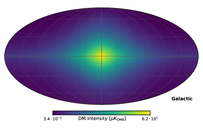
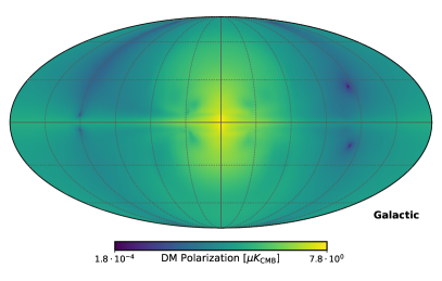
Fig. S3 shows the DM synchrotron maps for GHz for the intensity (left) and polarization amplitude (right), and for different GMF models (one for each row). The morphologies of the Sun+10 and Psh+11 DM intensity signal (left panels, first two rows) are both peaked at the Galactic Center and very similar, consistently with the fact that they use the same model for the random magnetic field, i.e., a double exponential. The JF12 model (left panel, lower row) instead predicts a more structured DM signal, with a bright peak at the Galactic center and other peaks in the Galactic plane reflecting the random field structure in the spiral arms. Overall, the JF12 model predicts a larger DM signal. This is explained by the larger field strength, see parameters in Ref.Jansson and Farrar (2012b) for more details. The morphology of the polarization amplitude signal is instead more complicated. The signal again peaks at the Galactic center, similarly to the intensity signal, but extends to higher latitudes following the ordered halo field. Again, the JF12 model predicts a larger signal away from the Galactic center, given the presence of a X-field and striated component on top of the disk and halo fields.
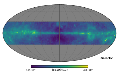
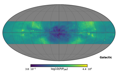
We show in Fig. S4 the map of the ratio between the Planck data at 30 GHz and a benchmark map for the annihilation of GeV into computed with the PDDE propagation and the Psh+11 model (so the same as the upper row in Fig. S3). Before computing the ratio, the error estimate for intensity and polarization has been added to the respective Planck data map. The lower value in the color map corresponds thus to our 68% C.L. upper limit, see main text. Since the DM signal and the backgrounds have different morphologies, the most constraining region does not coincide with the Galactic center, although the two signals both peak at the Galactic center. Instead, the most constraining pixels are located in a region various degrees above or below the Galactic Plane where the background is lower and the DM signal is still significant (compare with Fig. S3), providing the optimal signal to noise (S/N). For the polarization the optimal region is closer to the Galactic plane (GLON 358.2, GLAT 6.6 degrees) than in the case of the intensity (GLON 356.5, GLAT -14.8 degrees). This is due to the filamentary morphology of the polarization Planck map which leaves regions of low background in between the filaments very close to the Galactic center, contrary to the intensity case. This in part explains why polarization is more constraining than intensity regarding the DM signal.
Since we do not mask the microwave point sources in the map, their positions correspond to large values of log10(), and log10(), and thus weak DM constraints.
IV.2 Dark matter spectra
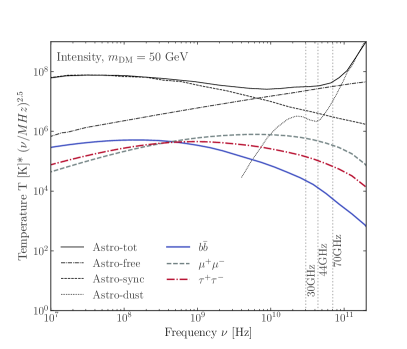
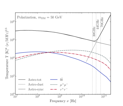
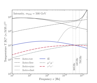
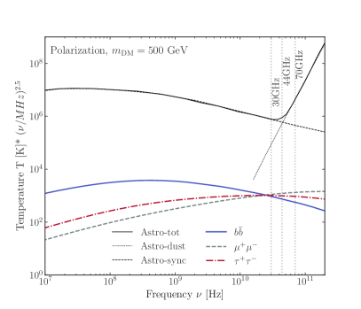
To illustrate the synchrotron spectra we explore a wide range of frequencies above and below the Planck LFI values in Fig. S5, for fixed masses of GeV (left and right panels, respectively) and the three benchmark annihilation channels. The spectrum of the polarization amplitude is very similar to the intensity one, with an overall smaller normalization value at the representative line of sight of (l,b)=(20,20)deg, at intermediate latitudes in the sky. At Planck LFI frequencies, an higher signal is expected in the leptonic channels, in particular in the . The hadronic channels might be better constrained using data at lower frequencies, see e.g. Ref. Cirelli and Taoso (2016).
For a tentative comparison, we include the spectra of the background emissions (’Astro’) as estimated in Ref. Orlando and Strong (2013) at high latitudes. Specifically, we take the total astrophysical emission which fits their multiwavelength dataset at high latitudes (right hand plots in their Figure 4), as well as the individual contributions estimated for synchrotron, dust, and free-free emission. For polarization below few tens of GHz, this is just the synchrotron contribution; for intensity, at the WMAP/Planck frequencies the free-free and spinning dust contributions are also important. As a further argument compelling our main results, we see that at the Planck frequencies the DM polarization signal is a factor 3-4 closer to the astrophysical emission derived in Ref. Orlando and Strong (2013) (which fits the data) with respect to the DM intensity. A computation of the astrophysical synchrotron intensity and polarization emission maps and spectra within the same sky region, propagation and GMF model is left to future work.
IV.3 Pixel size
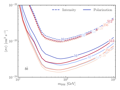
To investigate the effect of the pixel size in deriving DM upper limits with the Planck intensity and polarization maps we compute the constraints for different NSide values, from 16 to 512. For each resolution, the data and error maps are built as described in the main text, while the GALPROP prediction computed for NSide=512 is downgraded to low resolution using the healpy.ud_grade routine. We show the resulting upper limits for the synchrotron intensity (dashed lines) and the polarization amplitude (solid lines) as a function of the NSide value (line label, color scale from blue (16) to red (512)) in Fig. S6. The results are obtained fixing the PDDE propagation parameters, the Psh+11 GMF model and the annihilation channel. We first note that the DM constraints from intensity are only weakly dependent on the pixel size. This is consistent with the fact that the Planck measured intensity is in a regime of high S/N, as indeed can be seen comparing the intensity and error maps in Fig. 1. On the contrary Planck polarization has still a large noise and the pixel size has a larger impact on the DM constraints. A large pixel size increase the S/N at the price of losing the details of the morphology, while with a small pixel size the morphology of the signal is retained but with a lower S/N. As can be seen in Fig. S6, indeed, Nside 16 and NSide 512 provide the worst constraints while the optimal constraints are provided by the intermediate choice of NSide 128, i.e., for pixel mean spacing of about 0.5 deg, which is the one adopted for the results in the main text. We note, nonetheless, that even for the worst cases of Nside 16 and NSide 512 the polarization constraints are better than the intensity ones by a factor of 5, while in the optimal case of NSide 128 they are better by about one order of magnitude.
IV.4 Dark matter density profile
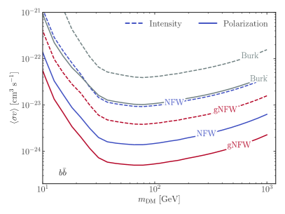
The effect of varying the DM density profile on the upper limits is illustrated in Fig. S7 (right panel). The blue lines refer to the benchmark NFW model, while the red and gray lines to the gNFW and Burkert cored profile, respectively. As it can be seen, the systematic uncertainty connected to the choice of the DM density profile is about one order of magnitude for both intensity and polarization. This is expected since the constraining power of our analysis comes from the Galactic center region (compare with Fig. S4), where the DM signal peaks, and in this region the different choices of profile differ significantly (see Fig. S7 left panel) giving large differences in the predicted DM signal. Our benchmark choice, the NFW profile, provides an intermediate result between the gNFW and the Burkert profile.

IV.5 Propagation parameters
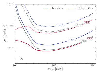
Another important systematic uncertainty for our DM upper limits is connected to the choice of the propagation setup. We illustrate the results for the three models we have employed in Fig. S8 (left). It can be seen that the limits differ in particular for low DM masses. Specifically, the DRE model, which is the only one with non-vanishing reacceleration, provides more stringent constraints at masses GeV. This is because the rather high Alfven velocity in the DRE model increases the density of low energy , and so their synchrotron emission, see Refs. Orlando (2018, 2019) for the corresponding propagated spectra at Earth. The PDDE propagation model provides the most conservative results among the explored models. Overall, the systematic uncertainty related to propagation effects is at the level of 20-30% for DM masses above 30 GeV.
IV.6 Upper limits for 44-70 GHz
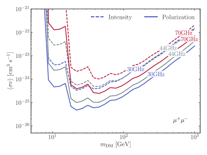
The upper limits computed using all the three Planck LFI frequency maps are illustrated in Fig. S8 (right panel) for the case of DM annihilating into pairs. The limits for 44 and 70 GHz are obtained following the same procedure as the GHz case. We find that the data at GHz provide the most constraining results in all the DM mass interval, with the only exception being a slight improvement for the GHz intensity case at masses larger than about 100 GeV. In principle, looking at the synchrotron emission spectrum in Fig. S5, an improvement of the limits at high DM masses for the leptonic annihilation channels is expected, especially for polarization, since the ratio of signal over background is increasing with increasing frequency, confront, e.g, the lower panels of Fig. S5 for the case GeV. In practice, however, the relative error on the Planck measured polarization increases significantly at 44 and 70 GHz (see maps in Figs.S1-S2) and this degrades the constraints at a level that makes the previous expectation not satisfied. We verified, indeed, that, when not considering the error estimation in the upper limit computation, the GHz frequencies are more constraining for GeV.
IV.7 Comparison with other works and probes
We show in Fig. S9 a comparison of our benchmark results (Psh+11 GMF, PDDE propagation, GHz Planck data) with representative upper limits obtained with similar or complementary probes of DM annihilation in our Galaxy and beyond. By exploiting the DM Galactic signal from synchrotron intensity only and early microwave data from WMAP and Planck , the authors of Ref. Egorov et al. (2016) (left panel, channel) and Ref. Cirelli and Taoso (2016) (right panel, channel) obtain results similar to our intensity constraints. Differences can be explained in terms of different choices of the GMF, propagation parameters and DM density profile, see the respective papers for more details. Results for the channel are not competitive with other DM targets and probes, such as traditional template fitting analysis of gamma-rays from dwarfs in Fermi-LAT data Albert et al. (2017) (see also more conservative, data-driven results presented in Ref. Calore et al. (2018)) or AMS-02 (limits taken from Ref. Kahlhoefer et al. (2021), comparable to other works, see e.g., Cuoco et al. (2017); Calore et al. (2022)). This is expected since the synchrotron signal probes mostly the leptonic annihilation channels. Indeed, our results using Planck polarization are competitive with Planck CMB constraints Aghanim et al. (2020b) between about 50 GeV and 100 GeV for the channel. This motivates further interest in going beyond the conservative approach presented in this paper.