Exploring and Validating Exoplanet Atmospheric Retrievals with Solar System Analog Observations

Abstract

Solar System observations that serve as analogs for exoplanet remote sensing data can provide important opportunities to validate ideas and models related to exoplanet environments. Critically, and unlike true exoplanet observations, Solar System analog data benefit from available high-quality ground- or orbiter-derived “truth” constraints that enable strong validations of exoplanet data interpretation tools. In this work, we first present a versatile atmospheric retrieval suite, capable of application to reflected light, thermal emission, and transmission observations spanning a broad range of wavelengths and thermochemical conditions. The tool — dubbed rfast — is designed, in part, to enable exoplanet mission concept feasibility studies. Following model validation, the retrieval tool is applied to a range of Solar System analog observations for exoplanet environments. Retrieval studies using Earth reflected light observations from NASA’s EPOXI mission provide a key proof-of-concept for under-development exo-Earth direct imaging concept missions. Inverse modeling applied to an infrared spectrum of Earth from the Mars Global Surveyor Thermal Emission Spectrometer achieves good constraints on atmospheric gases, including many biosignature gases. Finally, retrieval analysis applied to a transit spectrum of Titan derived from the Cassini Visual and Infrared Mapping Spectrometer provides a proof-of-concept for interpreting more feature-rich transiting exoplanet observations from NASA’s James Webb Space Telescope (JWST). In the future, Solar System analog observations for exoplanets could be used to verify exoplanet models and parameterizations, and future exoplanet analog observations of any Solar System worlds from planetary science missions should be encouraged.

1 Introduction

Atmospheric remote sensing has proven essential to interpreting exoplanet observations (Madhusudhan, 2018; Fortney et al., 2021), with applications ranging from some of the first-ever potential constraints on the composition of exoplanet atmospheres (Tinetti et al., 2007; Pont et al., 2008; Swain et al., 2008; Sing et al., 2009; Bean et al., 2010) through to the more-modern atmospheric retrieval (or inverse modeling) approaches developed in a wide range of studies (Irwin et al., 2008; Madhusudhan & Seager, 2009; Line et al., 2012; Benneke & Seager, 2012; Line et al., 2013, 2014; Kreidberg et al., 2014; Knutson et al., 2014; Stevenson et al., 2014; Morley et al., 2016; Barstow et al., 2017; MacDonald & Madhusudhan, 2017; Tsiaras et al., 2019; Mollière et al., 2019; Benneke et al., 2019; Zhang et al., 2019; Kitzmann et al., 2020; Colón et al., 2020; Min et al., 2020; Mansfield et al., 2022). In the very near future, atmospheric retrieval tools are likely to see widespread application to exoplanet observations from NASA’s JWST (Cowan et al., 2015; Greene et al., 2016; Krissansen-Totton et al., 2018; Nixon & Madhusudhan, 2022). Inverse modeling tools are also likely to prove key when interpreting exoplanet observations from near-future exoplanet-themed missions, such as NASA’s Nancy Grace Roman Space Telescope (Roman; Akeson et al., 2019; Kasdin et al., 2020; Marley et al., 2014; Lupu et al., 2016; Nayak et al., 2017) and ESA’s Ariel mission (Tinetti et al., 2016; Barstow et al., 2022).

Recommendations from the recent Decadal Survey on Astronomy and Astrophysics 2020 indicate that studies of exoplanet environments should continue to expand in both quantity and quality, engaging complementary ground- and space-based resources. When looking forward to future exoplanet exploration strategies, atmospheric inverse modeling will play at least two major roles. First, and most obviously, atmospheric retrieval tools will be needed to interpret data from any near- or far-future observing facilities and characterize exoplanet properties. Second, and maybe less obviously, inverse models can provide the connection between proposed instrument/telescope performance and the expected constraints on the parameters that describe an exoplanet environment. In fact, atmospheric retrieval is actively being used to refine designs of the Habitable Exoplanet Observatory (HabEx; Gaudi et al., 2018), the Large UltraViolet-Optical-InfraRed Surveyor (LUVOIR; Roberge & Moustakas, 2018), and the Origins Space Telescope (Battersby et al., 2018) mission concepts (or their successors; Feng et al., 2018; Smith et al., 2020; Tremblay et al., 2020; Damiano & Hu, 2021).

Given the large number of exoplanet-themed missions and instruments, either operational or on the horizon, it may be easy to become focused on environments that are many parsecs away from Earth. Such an outlook can miss important opportunities that Solar System worlds present for guiding exoplanet science (Roberge et al., 2017; Keithly & Savransky, 2021). For example, Solar System planets and moons can serve as models for the predicted appearance of analogous exoplanet targets (Tinetti et al., 2005, 2006; Stam, 2008; Kaltenegger & Traub, 2009; Zugger et al., 2010; Robinson et al., 2011; Fujii et al., 2014; Robinson et al., 2014; Dalba et al., 2015; Mayorga et al., 2016; Lustig-Yaeger et al., 2018; Macdonald & Cowan, 2019; Kane et al., 2019; Mayorga et al., 2020, 2021).

From the perspective of exoplanet atmospheric remote sensing, Solar System worlds and observations can yield opportunities to both validate retrieval model results and capabilities and to test the simplifying parameterizations necessarily adopted in these tools. A recent review of connections between Solar System planetary science and exoplanet science (Kane et al., 2021) highlighted measurables from Solar System worlds as a “pathway forward” for more-correct interpretations of exoplanet data. However, relatively few works have examined such applications of Solar System observations. Marley et al. (2014) (and a more-formal companion study, Lupu et al., 2016), in exploratory work relevant to (what is now) Roman, performed retrievals on visible-wavelength observations of Jupiter, Saturn, and Uranus (from Karkoschka, 1998) and demonstrated that methane abundances could be reliably inferred using a forward model that included two distinct cloud decks. The assumption of grey cloud properties was found to be generally acceptable, although haze absorption at wavelengths shorter than those considered in the study would be an important consideration for future mission concepts. Heng & Li (2021) used high-quality phase curves of Jupiter from the Cassini Imaging Science Subsystem (Porco et al., 2004; Li et al., 2018) to infer properties of Jovian clouds with potential implications for JWST. Finally, Tribbett et al. (2021) performed retrievals on effective transit spectra of Titan — generated from stellar occultations observed by the Cassini Ultraviolet Imaging Spectrograph (Esposito et al., 2004; Koskinen et al., 2011) — and showed that simple parameterizations of haze extinction failed to detect the presence of known haze layers/over-densities.

The work that follows explores a variety of novel retrieval studies for Solar System worlds treated as exoplanet analogs, which is a strongly under-explored area of study. Section 2 develops a versatile and efficient inverse modeling suite whose origins stem from exoplanet direct imaging mission concept studies. Validations against existing tools are showcased in Section 3. Section 4 first demonstrates an application to direct imaging studies of Earth-like exoplanets and subsequently demonstrates retrieval results as applied to disk-integrated reflected light observations of Earth, disk-integrated infrared observations of Earth, and near-infrared transit spectra of Titan. Key findings from these retrieval studies are discussed in the context of near- and further-future exoplanet-themed missions in Section 5 while take-away findings are enumerated in Section 6.

2 Methods

Atmospheric retrieval (or inference) requires a suite of interconnected tools: a parameter space sampling tool, a radiative transfer “forward” model, and an instrument model. When retrieving on a noisy observation, the sampling tool uses information about goodness of fit to statistically explore a posterior distribution for a collection of atmospheric and planetary parameters (i.e., “state” vectors). For a particular instance of a state vector, the radiative transfer model, in general, predicts a high resolution spectrum that is subsequently spectrally degraded to match the resolution of the observed spectrum via the instrument model. A likelihood comparison between the observed spectrum and the degraded prediction then enables the sampling algorithm to further explore posterior space. For mission design purposes — where true observations do not yet exist — it is often the case that faux/synthetic observations must be generated using a forward model and an instrument model. Adopting this faux observation into the retrieval framework then enables exploration of how changes to key mission/instrument parameters map to changes in expected constraints on planetary environments.

Material below describes the components of a computationally efficient, open source, and user friendly generalized atmospheric retrieval package, called rfast. Core elements of the rfast package were developed to support studies for the HabEx and LUVOIR mission concepts. Direct imaging capabilities were inspired by a rocky exoplanet retrieval tool described in Feng et al. (2018), although many changes and upgrades have been introduced: opting for a fully Python-based implementation rather than merged Python/Fortran, allowing for a wider variety of atmospheric gases (and, thus, planet types) with both pressure- and temperature-dependent opacities, and enabling users to straightforwardly toggle on/off which atmospheric and planetary parameters should be included in the retrieval analysis and what priors should be adopted for these parameters. Other notable model capabilities include treatments for vertically-varying gas and temperature profiles and the ability to divide a synthetic spectrum into bands with distinct wavelength coverages, noise levels, and spectral resolutions. Finally, to enable both mission concept and feasibility studies beyond reflected light direct imaging scenarios, the rfast suite also includes options for spectroscopic studies in thermal emission, combined reflected light and thermal emission, and transit transmission.

2.1 Reflected Light Forward Model

The rfast tool includes treatments of reflected light spectroscopy and photometry where the planet is either treated as a single plane-parallel scene (one-dimensional) or as a pixelated globe (three-dimensional). Radiative transfer for each pixel in the three dimensional treatment makes a local plane-parallel assumption and thereby allows for simulated observations that depend on planetary phase angle. While the single scene option does not allow for phase-dependent studies, the reduction from three dimensional to one dimensional geometry retains suitability for broad mission concept studies while also offering large computational efficiency improvements (i.e., usually at least an order of magnitude improvement in runtime).

Radiative transfer in the single scene option follows a diffuse two-stream flux adding treatment developed in Robinson & Crisp (2018). For each model layer, layer reflectivity ($r_{k}$) and transmissivity ($t_{k}$) terms are computed by integrating the hemispheric mean two-stream radiative transfer equations over optical depth assuming a diffuse illumination source, yielding,

$$r_{k}=\frac{A_{\infty}\left(1-e^{-2a_{k}b_{k}\Delta\tau_{k}}\right)}{1-A_{\infty}^{2}e^{-2a_{k}b_{k}\Delta\tau_{k}}}~{}~{}~{}\left(0\leq\omega_{k}<1\right)\ ,$$ (1)

$$t_{k}=\frac{\left(1-A_{\infty}^{2}\right)e^{-a_{k}b_{k}\Delta\tau_{k}}}{1-A_{\infty}^{2}e^{-2a_{k}b_{k}\Delta\tau_{k}}}~{}~{}~{}\left(0\leq\omega_{k}<1\right)\ ,$$ (2)

with $a_{k}=\sqrt{1-\omega_{k}}$, $b_{k}=\frac{3}{2}\sqrt{1-w_{k}g_{k}}$, and $A_{\infty}=(\frac{2}{3}b_{k}-a_{k})/(a_{k}+\frac{2}{3}b_{k})$. Here, $\Delta\tau_{k}$ is the layer extinction optical depth, $\omega_{k}$ is the layer single scattering albedo, $g_{k}$ is the layer scattering asymmetry parameter, and $A_{\infty}$ is the layer reflectivity as the optical depth tends to infinity, all of which can generally depend on wavelength. A single scattering albedo of unity represents a special case where,

$$r_{k}=\frac{\frac{3}{4}(1-g_{k})\Delta\tau_{k}}{1+\frac{3}{4}(1-g_{k})\Delta\tau_{k}}~{}~{}~{}(\omega_{k}=1)\ ,$$ (3)

$$t_{k}=\frac{1}{1+\frac{3}{4}(1-g_{k})\Delta\tau_{k}}~{}~{}~{}(\omega_{k}=1)\ .$$ (4)

The reflectivity of the inhomogeneous atmospheric column extending upward from the surface is then determined via a recursive relation,

$$R_{k}=r_{k}+\frac{t_{k}^{2}R_{k+1}}{1-r_{k}R_{k+1}}\ ,$$ (5)

where $R_{k}$ is the reflectivity of the atmospheric column extending from the surface to the top of the $k$-th layer (i.e., so that $R_{1}$ can be taken as the planetary reflectivity in the single scene model). The lower boundary condition for a model with $N$ atmospheric levels is applied as $R_{N}=A_{\rm s}$, where $A_{\rm s}$ is the wavelength-dependent surface albedo.

The phase-dependent option adds a treatment for the direct solar beam that follows Hapke (1981). In each pixel, radiation scattered in a given layer that does not remain in the direct beam enters the diffuse field and is included in layer flux upwelling and downwelling source terms ($s_{j}^{+}$ and $s_{j}^{-}$, respectively). The fraction of the diffuse flux that enters either the upwelling or downwelling source terms is determined via integrating the scattering phase function over the upwelling and downwelling directions given the pixel illumination geometry. Given the layer source terms and the layer reflectivity and transmissivity (which only apply to the diffuse field), the diffuse flux traveling upward at the top of the atmospheric pixel is determined using Equations (4), (5), and (7–9) in Robinson & Crisp (2018). Combining the diffuse flux with the emergent direct beam intensity yields the total emergent intensity from a plane-parallel pixel.

Summation over the pixelated disk is accomplished using Gauss-Chebyshev integration, as detailed in Horak & Little (1965). For a model with spatial degree $M$, the Gauss points and weights ($x_{{\rm G},i}$ and $w_{{\rm G},i}$, respectively) are based on the roots of the Legendre polynomials of degree $M$, while the Chebyshev points and weights ($x_{{\rm C},j}$ and $w_{{\rm C},j}$) are based on the Chebyshev polynomials of the first kind (see Section 2 of Webber et al., 2015). The cosine of the solar and observer zenith angles for a given pixel are then given, respectively, by,

$$\mu_{\rm s,ij}=\sin\left(\cos^{-1}x_{{\rm C},j}\right)\cos\left(\zeta_{i}-\alpha\right)\ ,$$ (6)

$$\mu_{\rm o,ij}=\sin\left(\cos^{-1}x_{{\rm C},j}\right)\cos\left(\zeta_{i}\right)\ ,$$ (7)

where $\alpha$ is the planetary phase angle and,

$$\sin\zeta_{i}=\frac{\cos\alpha+1}{2}\left(x_{{\rm G},i}-\frac{\cos\alpha-1}{\cos\alpha+1}\right)\ .$$ (8)

Given this formalism, the flux emerging from the spatially integrated disk is,

$$F_{\lambda}\left(\alpha\right)=\frac{\cos\alpha+1}{2}\sum_{i=1}^{M}\sum_{j=1}^{M}w_{{\rm G},i}w_{{\rm C},j}I_{\lambda}\left(\tau=0;\alpha,\mu_{\rm s,ij},\mu_{\rm o,ij}\right)\ ,$$ (9)

where $I_{\lambda}\left(\tau=0;\alpha,\mu_{\rm s,ij},\mu_{\rm o,ij}\right)$ is the wavelength-dependent specific intensity emerging from the $ij$-th pixel at the given planetary phase angle. The number of pixels on the illuminated disk scales as $M^{2}$ and spatially homogeneous models can halve the number of Chebyshev points due to a symmetry about the illumination equator. Adopting a normal-incidence top-of-atmosphere specific stellar flux of unity causes Equation 9 to yield the wavelength-dependent planetary geometric albedo ($A_{\rm g}$) at full phase ($\alpha=0$) and the product of the geometric albedo and the planetary phase function ($\Phi\left(\alpha\right)$) at other phase angles.

2.2 Emitted Light Forward Model

Treatments for emitted light spectra are similar to the single scene reflected light model. Layer reflectivity and transmissivity are computed as in the reflected light case, and it is useful to define a layer absorptivity,

$$a_{k}=1-r_{k}-t_{k}\ .$$ (10)

Following Robinson & Crisp (2018), layer thermal flux source terms in the upwelling and downwelling directions are given by,

$$s_{k}^{+}=\pi\left[a_{k}B_{\lambda}\left(T_{k}\right)-\delta B_{\lambda,k}\right]\ ,$$ (11)

$$s_{k}^{-}=\pi\left[a_{k}B_{\lambda}\left(T_{k+1}\right)+\delta B_{\lambda,k}\right]\ ,$$ (12)

where $B_{\lambda}$ is the Planck function, $T_{k}$ is the temperature at level $k$ (incrementing downward), and,

$$\delta B_{\lambda,k}=\left(1-a_{k}+\frac{a_{k}}{1-a_{k}}\right)\left[B_{\lambda}\left(T_{k}\right)-B_{\lambda}\left(T_{k+1}\right)\right]\ ,$$ (13)

which is a correction that ensures the net thermal flux across a layer tends towards the radiation diffusion limit for large optical depths. Lower boundary conditions use a surface emissivity and a Planck-like surface emission term while the upper boundary condition is zero incident downwelling thermal radiation. Upwelling thermal flux at the top of the planetary atmosphere is determined using the flux adding expressions in Equations (4), (5), and (7–9) of Robinson & Crisp (2018).

2.3 Transit Spectroscopy Forward Model

Transit spectra are computed in the geometric limit (i.e., assuming straight line ray trajectories) using the one-dimensional path distribution approach developed by Robinson (2017) (see also MacDonald & Lewis, 2021). For an atmospheric layer centered at radial distance $r_{k}$ with width $\Delta r_{k}$, and for a ray incident on the atmosphere with impact parameter $b$, the geometric path distribution is given by,

$$\mathcal{P}_{b}\!\left(r_{k}\right)=\begin{cases}0\ ,&b\geq r_{k}+\Delta r_{k}/2\\ \frac{2}{\Delta r_{k}}\sqrt{\left(r_{k}+\Delta r_{k}/2\right)^{2}-b^{2}}\ ,&r_{k}-\Delta r_{k}/2<b<r_{k}+\Delta r_{k}/2\\ \frac{2}{\Delta r_{k}}\left[\sqrt{\left(r_{k}+\Delta r_{k}/2\right)^{2}-b^{2}}-\sqrt{\left(r_{k}-\Delta r_{k}/2\right)^{2}-b^{2}}\right]\ ,&b\leq r_{k}-\Delta r_{k}/2\ .\\ \end{cases}$$ (14)

For an atmospheric model with $N$ levels and assuming that the grid of impact parameters corresponds to layer midpoints, the geometric path distribution is a matrix of size $N-1\times N-1$. Given a vector of layer differential optical depths, $\boldsymbol{\Delta\tau}$, the wavelength-dependent slant path transmissivity, $\boldsymbol{t}$, for each impact parameter can be computed using matrix algebra with,

$$\boldsymbol{t}=\boldsymbol{1}-\boldsymbol{a}={\rm{EXP}}\!\left(-\boldsymbol{\Delta\tau}\cdot\boldsymbol{\mathcal{P}}\right)\ ,$$ (15)

where we have defined the absorptivity vector, $\boldsymbol{a}$. If we define a vector of annulus areas as $A_{k}=2\pi b_{k}\Delta b_{k}$, then the wavelength dependent transit spectrum can be written as,

$$\left(\frac{R_{\rm{p},\lambda}}{R_{\rm{s}}}\right)^{\!\!2}=\frac{1}{R_{\rm{s}}^{2}}\left(R_{\rm{p}}^{2}+\frac{1}{\pi}\boldsymbol{a}\cdot\boldsymbol{A}\right)\ ,$$ (16)

where $R_{\rm p}$ is a reference planetary radius (e.g., the solid body radius or the radius at a specified atmospheric pressure) and $R_{\rm s}$ is the host stellar radius.

Transit spectra in the rfast tool are generally treated in the pure absorption limit, so that the optical depths adopted in the expressions above are extinction optical depths. For particles, aerosol forward scattering — which can reduce slant path optical depths — is treated using the analytic formalism of Robinson et al. (2017). A refractive floor to the transit spectrum follows existing analytic treatments (Sidis & Sari, 2010; Bétrémieux & Kaltenegger, 2014; Robinson et al., 2017).

2.4 Other Model Considerations

The relationship between pressure and altitude — which is especially important for transit spectroscopy — is determined by solving the hydrostatic equation given the atmospheric thermal and chemical state. Assuming that gravitational acceleration is proportional to $\left(R_{\rm p}+z\right)^{2}$ (where $z$ is altitude above the planetary radius) and that temperature varies linearly with pressure through a layer yields the recursion,

$$\frac{R_{\rm p}}{1+z_{k}/R_{\rm p}}=\frac{R_{\rm p}}{1+z_{k+1}/R_{\rm p}}-h_{k}$$ (17)

with,

$$h_{k}=\frac{k_{\rm B}}{g_{\rm s}m_{k}}\left[\left(T_{k+1}-\frac{T_{k}-T_{k+1}}{p_{k}-p_{k+1}}\right)\ln\frac{p_{k+1}}{p_{k}}-T_{k}+T_{k+1}\right]\ ,$$ (18)

where $k_{\rm B}$ is Boltzmann’s constant, $g_{\rm s}$ is the acceleration due to gravity at $R_{\rm p}$ (e.g., at the planetary surface), $m$ is the layer mean molecular mass, and $T$ and $p$ are the level-dependent temperature and pressure, respectively. The acceleration due to gravity at any altitude is simply,

$$g\left(z\right)=\frac{g_{\rm s}}{\left(1+z/R_{\rm p}\right)^{2}}\ .$$ (19)

Unless otherwise noted, molecular opacities are derived from the HITRAN database (Gordon et al., 2022) using the Line-By-Line ABSorption Coefficients tool (LBLABC; Meadows & Crisp, 1996). The rfast radiative transfer tools can also interface to the Freedman et al. (2008) opacities database (see also Freedman et al., 2014). Full line-resolving opacities are placed onto a wavenumber grid at 1 cm^-1 resolution (0.1 cm^-1-resolved opacities are also available for high-resolution applications) and then further degraded in resolution when forward or inverse modeling to at least an order of magnitude finer resolving power than the relevant observational data. For each incorporated molecule, opacities span 0.1–100 $\upmu$m so that the highest resolving power that can be accommodated (assuming no over-sampling) at optical/near-infrared/thermal wavelengths is roughly 10,000/2,000/100. As the core radiative transfer solvers for rfast are indifferent to thermochemical conditions, the input opacities are then the only determinant of the types of worlds that can be simulated using the rfast suite. Cold and clement worlds are emphasized below, so the adopted opacities span only 50–700 K. Nevertheless, LBLABC-generated opacities have been shown to compare well to other tools even under hot Jupiter-like conditions (Robinson, 2017).

A primary design consideration for the rfast tool is rapid exploration of retrieval scenarios. Software is nearly entirely written using linear algebra techniques, thereby taking advantage of vectorized computational approaches. Exceptions occur for aspects of atmospheric recursion relations and integration over atmospheric pixels in the three-dimensional reflected light option. As the number of atmospheric levels or planetary pixels are generally at least 1–2 orders of magnitude smaller than the number of spectral points, these exceptions do not impart any significant model inefficiencies. On a single processor, the rfast tool can generate a spectrum with 10k spectral points for a model atmosphere with 50 vertical levels and eight absorbing gas species (including opacity interpolation over both pressure and temperature) in 400 ms for the single scene reflectance option, 1 s for the three-dimensional phase-dependent reflectance option (with $M=3$), 600 ms for the thermal emission option, and 300 ms for the transit spectroscopy option.

The rfast model currently adopts the widely-used and versatile emcee Markov chain Monte Carlo sampler (Foreman-Mackey et al., 2013) when employed as a retrieval tool. Functions for computing the likelihood, prior probability, and posterior probability could straightforwardly be adapted for use with analogous samplers, and efficiencies may be gained by adopting a multi-nested sampling routine (Buchner et al., 2014). The rfast framework allows for retrieving on more than 20 atmospheric, planetary, and orbital parameters: atmospheric surface pressure, atmospheric temperature, surface albedo, atmospheric mean molar weight, planetary radius, planetary mass, surface gravity, cloud top pressure, cloud vertical extent, cloud optical thickness, fractional cloudiness, orbital distance, planetary phase angle, as well as gas mixing ratios for argon, molecular nitrogen, molecular oxygen, water vapor, carbon dioxide, ozone, carbon monoxide, nitrous oxide, methane, helium, and molecular hydrogen. Users may adopt uninformed or Gaussian priors in either log or linear space. Additionally, gas abundance retrievals may be performed with the center-log ratio approach, which has been adapted in exoplanet applications to prevent biased priors for a background gas in Benneke & Seager (2012) (see also Damiano & Hu, 2021; Piette et al., 2022).

3 Model Validations

Theoretical aspects of the rfast forward model have already seen applications in various Solar System and exoplanet studies, although implementations there were Fortran-based (Robinson et al., 2011; Robinson, 2017; Robinson & Crisp, 2018). Nevertheless, the novel applications within the rfast framework warrant validation. Importantly, aspects of core radiative transfer engines as well as overall forward modeling capabilities require verification. Finally, the retrieval capabilities of the rfast suite can be verified against a key initial investigation into atmospheric inference for directly imaged Earth-like exoplanets (Feng et al., 2018).

3.1 Isochromatic Core Radiative Transfer Model Validations

A standard check of the radiative properties of a single homogeneous atmospheric layer (i.e., a layer with uniform optical properties throughout) is to compare against the detailed numerical solutions of Hunt (1973). In this earlier work, the flux reflectivity, transmissivity, and emissivity (analogous to $r_{k}$, $t_{k}$, and $a_{k}$ in this present work) were studied for layers of various optical thickness and constant single scattering albedo and asymmetry parameter. Figure 1 compares results from the Hunt (1973) study to those from the rfast two-stream treatment for two limiting cases — pure absorption and forward scattering. While systematic biases are apparent, these are equivalent to other two-stream approaches (Toon et al., 1989). More specifically, reflectivity and transmissivity biases are comparable in magnitude and direction to those reported in Toon et al. (1989). Emissivity biases can be large (greater than 10%) for cases with small optical depths (i.e., optical depths below a few tenths), and two-stream models presented in Toon et al. (1989) also struggle in these conditions. Note that these layer properties underpin the single scene reflectance and thermal emission options in rfast as well as the treatment of multiply-scattered radiation in the phase-dependent option.

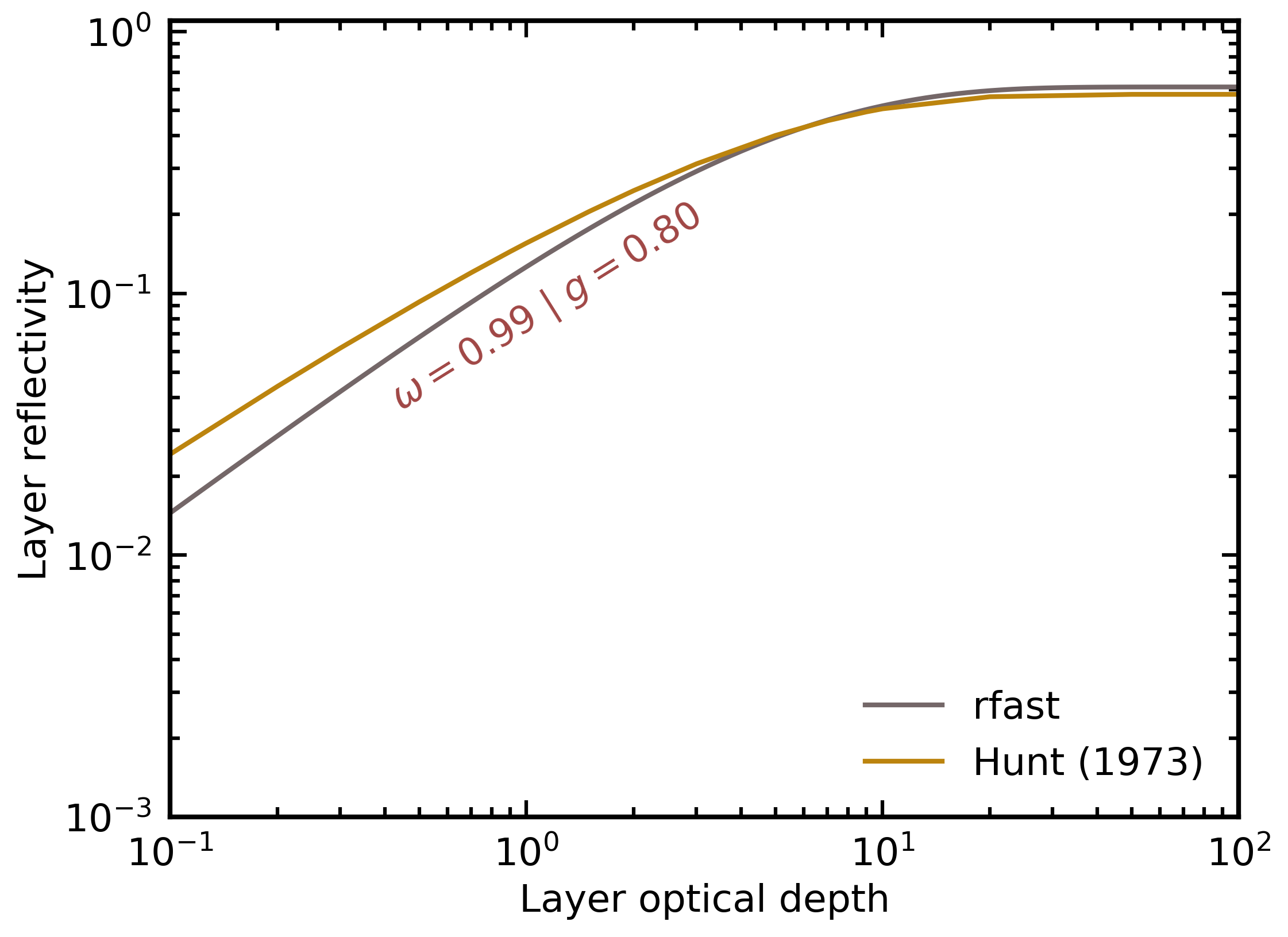
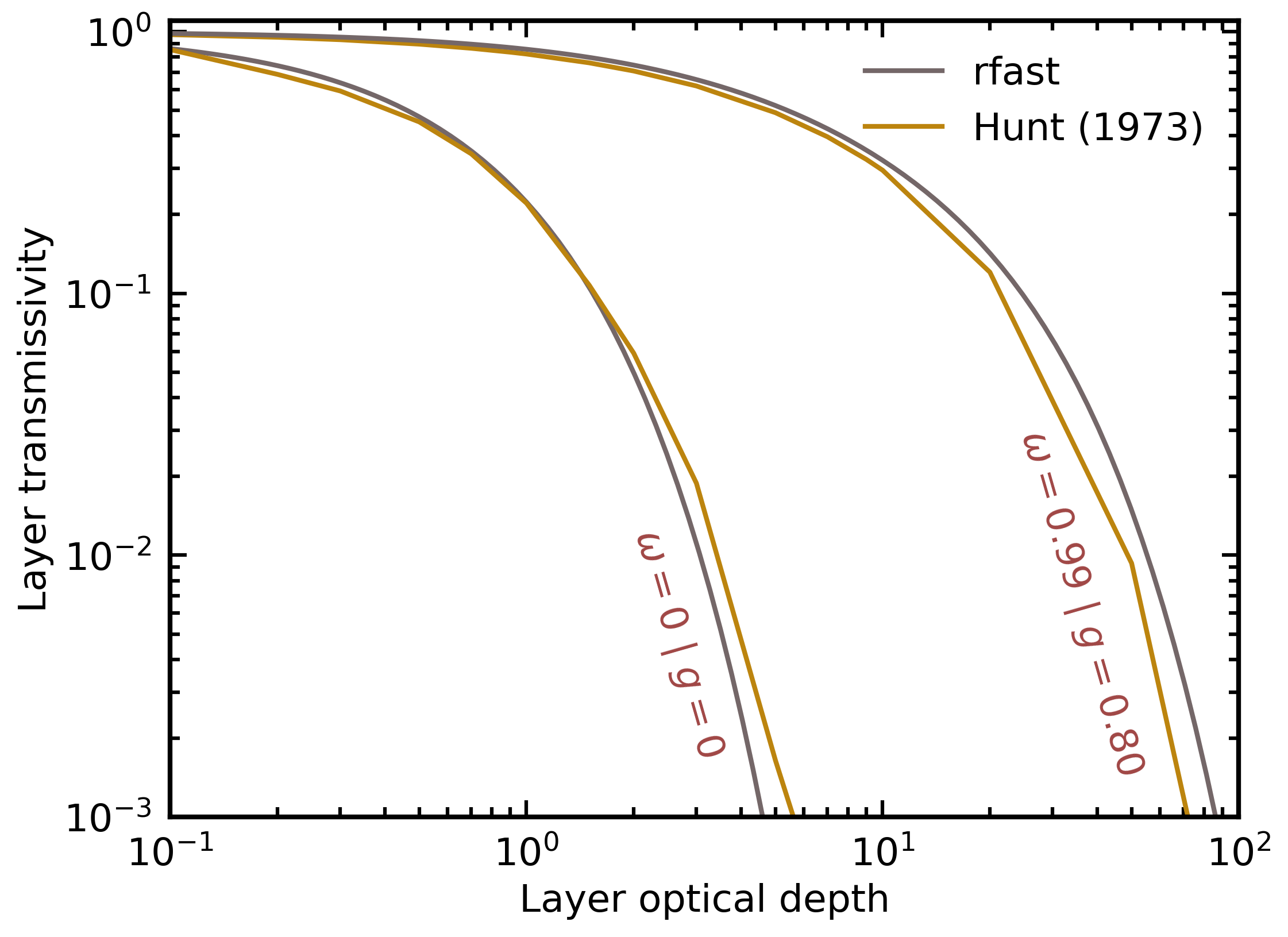
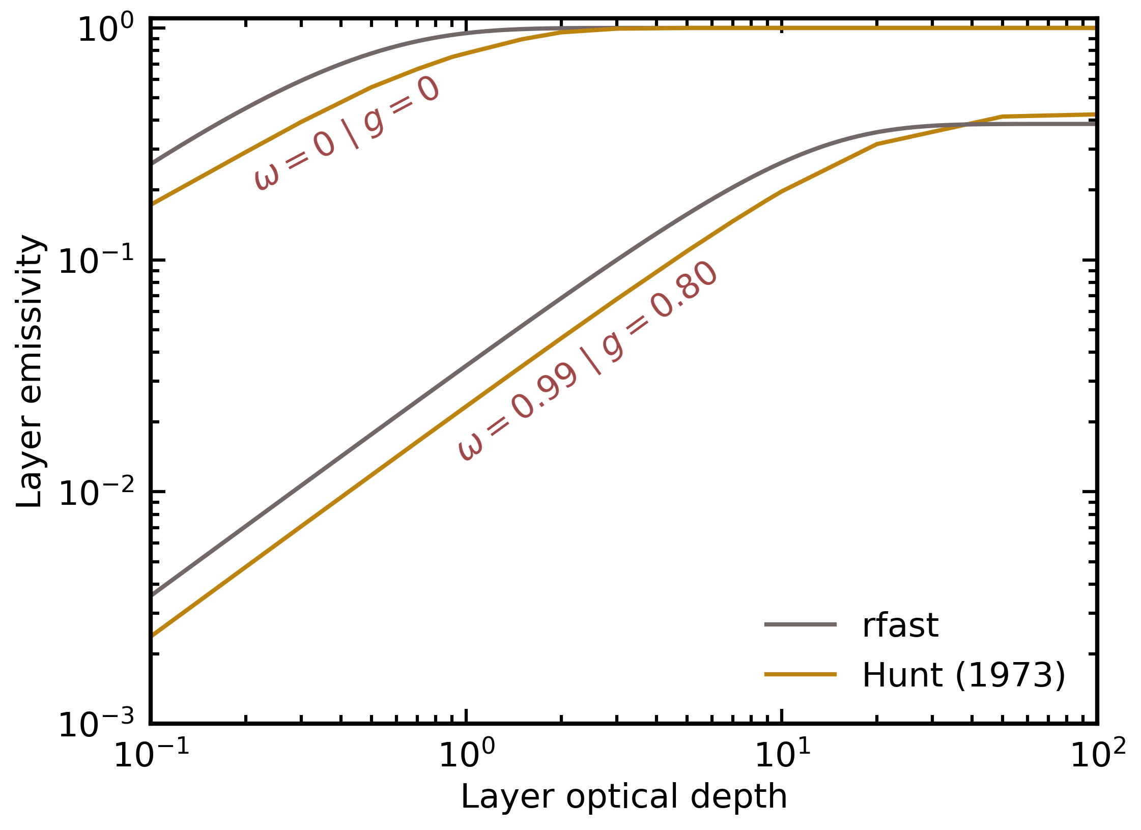
Figure 1: Layer reflectivity (top left), transmissivity (top right), and emissivity (bottom) as a function of layer extinction optical depth in the rfast model (grey lines) versus detailed calculations from Hunt (1973) (yellow lines). Limiting cases of pure absorption and forward scattering are considered, where layers have no reflectivity in the pure absorption case.

The theoretical study of the phase-dependent reflection of planetary bodies with homogeneous atmospheres has a long history (Horak, 1950; Sobolev, 1975). More recent studies provide straightforward opportunities to validate phase-dependent treatments within rfast — both Madhusudhan & Burrows (2012) and Heng et al. (2021) present analytic or near-analytic results for light reflection from planetary bodies with homogeneous atmospheres (or surfaces) that have different scattering properties. Figure 2 compares phase-dependent reflectance values (i.e., the product of the geometric albedo and planetary phase function) from the Madhusudhan & Burrows (2012) work to those from rfast for (optically) infinitely deep Rayleigh and isotropically scattering cases. A Lambertian surface case (where the phase-dependent reflectance has an analytic solution) is well-reproduced by rfast so is not shown. Similarly, Figure 3 compares results from Heng et al. (2021) and rfast for the planetary geometric albedo and spherical albedo ($A_{\rm s}$) as a function of single scattering albedo for an infinitely deep atmosphere whose medium has a Henyey-Greenstein phase function of asymmetry parameter $g=0.508$ (Henyey & Greenstein, 1941). (Note that the planetary spherical albedo is given by the integral of $A_{\rm g}\phi\left(\alpha\right)\sin\alpha$ over all phase angles.) All phase-dependent validations adopt $M=10$ for Gauss-Chebyshev integration, which was shown to provide better than 1% precision. Discrepancies between rfast and the more-sophisticated calculations do occur for geometric albedo and reflectivity calculations (which are most relevant to reflected light observations) at the level of 10% (or more, under some circumstances), which stems from the simplifying assumption of hemispheric mean radiative transfer in the multiply-scattered radiation field. Future work could incorporate more-accurate radiative transfer solvers that still maintain high computational efficiency (e.g., Spurr & Natraj, 2011). As described in Section 5, this precludes some phase-dependent retrievals on observational data, but does not preclude retrievals performed on phase-dependent synthetic observations generated with rfast.

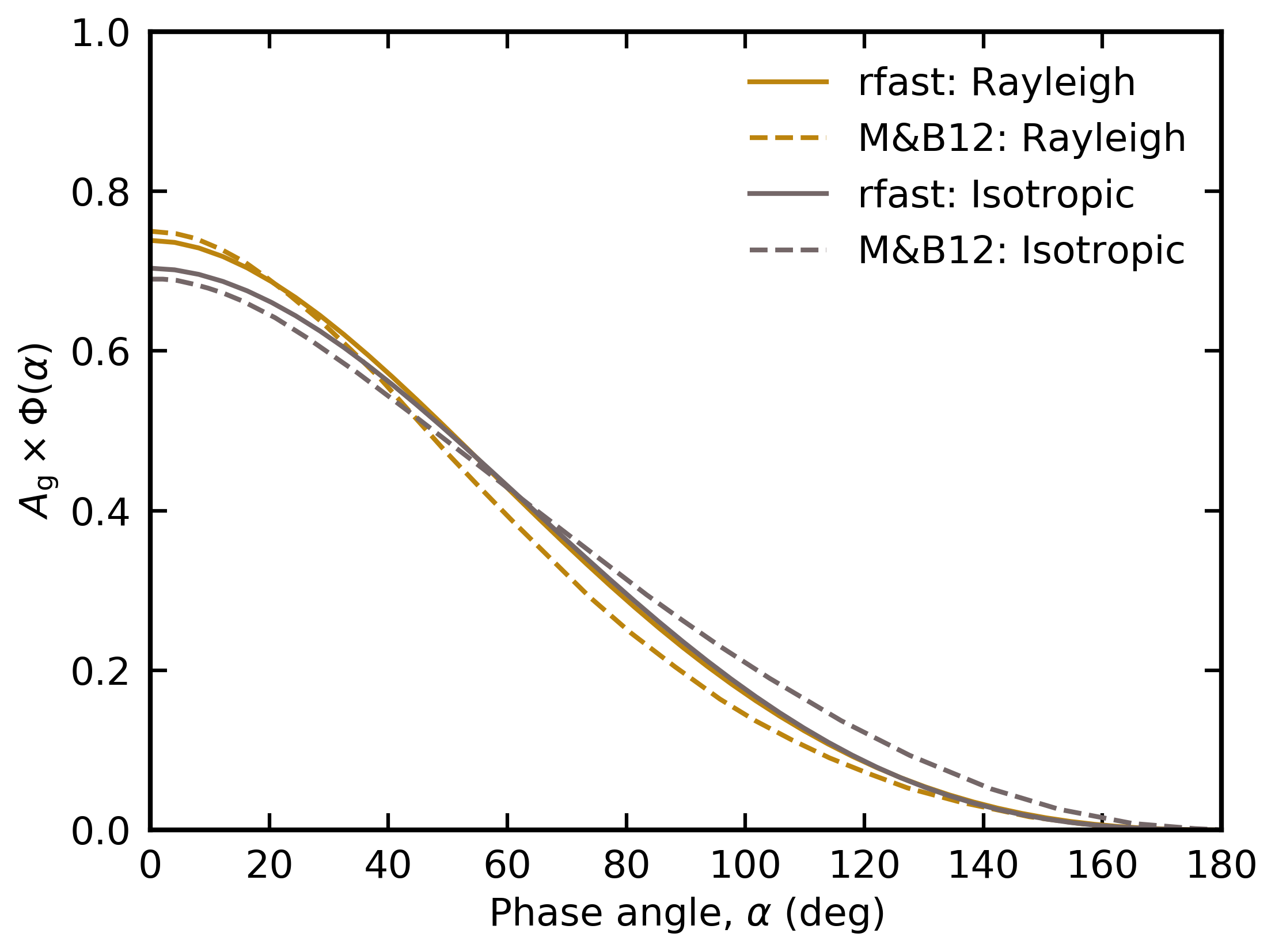
Figure 2: Phase-dependent planetary reflectivity for infinitely deep Rayleigh and isotropic scattering atmospheres from Madhusudhan & Burrows (2012) as compared to rfast.

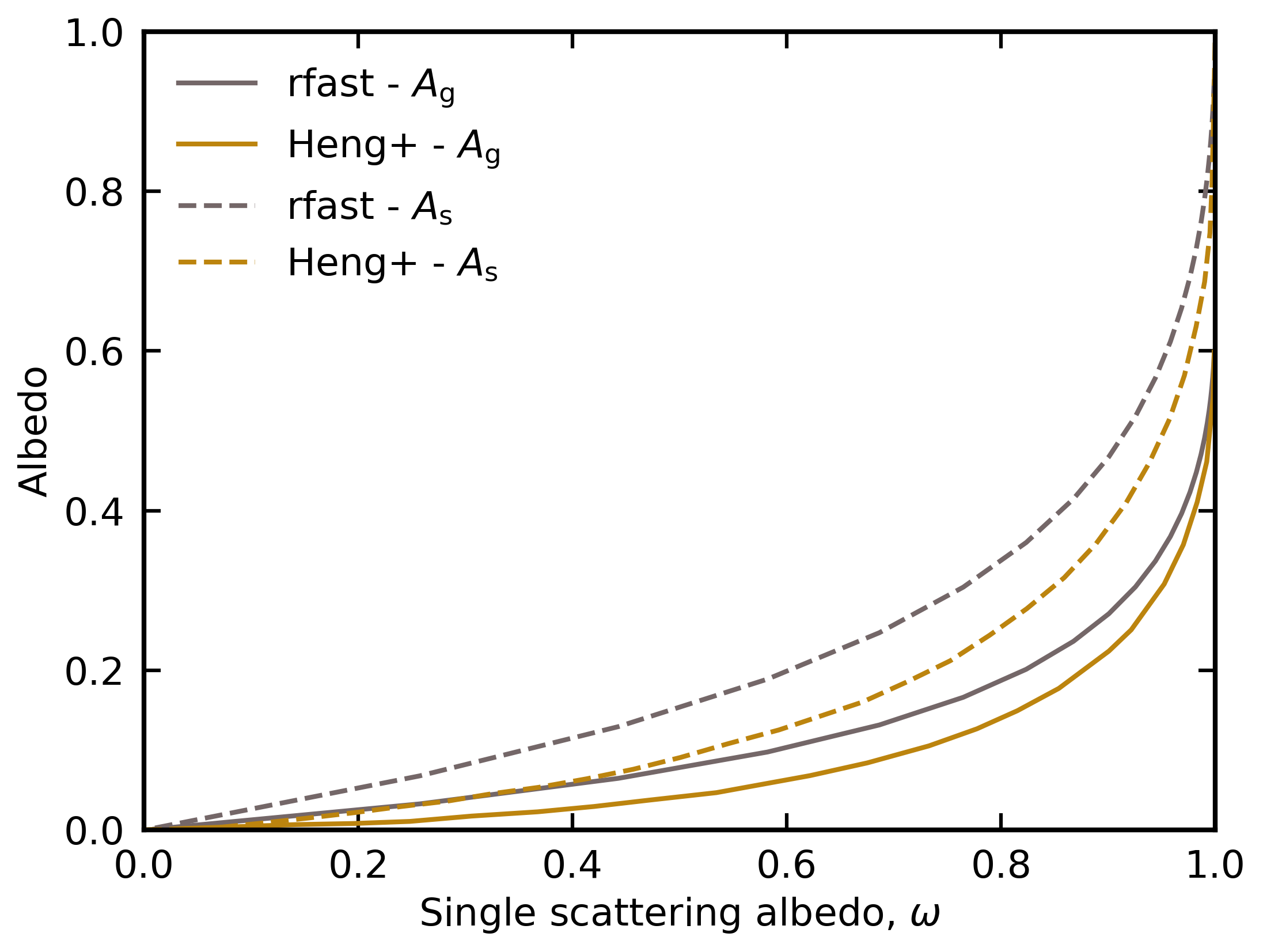
Figure 3: Planetary geometric ($A_{\rm g}$; solid lines) and spherical ($A_{\rm s}$; dashed lines) albedo as a function of single scattering albedo from Heng et al. (2021) and rfast for an infinitely deep atmosphere whose medium obeys a Henyey-Greenstein scattering phase function of asymmetry parameter 0.508 (selected to reproduce population-level results for hot Jupiters by Heng et al., 2021).

3.2 Spectral Validations

The primary utility of the rfast tool is in generating spectra, so spectral validations are of central importance. Comparisons/validations in reflected or emitted light presented here are against the plane-parallel, line-by-line, multiple scattering Spectral Mapping Atmospheric Radiative Transfer (SMART) model (developed by D. Crisp; Meadows & Crisp, 1996) while transit spectrum comparisons are against the scaTran addition to SMART (Robinson, 2017). Phase-dependent SMART results come from a disk integration technique developed in Robinson et al. (2011). All comparisons adopt a standard Earth atmospheric model (McClatchey et al., 1972) and include gas opacity from N₂, O₂, H₂O, CO₂, O₃, CO, CH₄, and N₂O.

Figure 4 compares results from plane-parallel SMART and single-scene rfast, both at a resolving power ($\lambda$/$\Delta\lambda$) of 200. Simulations with both rfast and SMART include 50% coverage of water ice and liquid clouds with realistic wavelength-dependent scattering properties and a Henyey-Greenstein phase function. The SMART simulation adopts a solar zenith angle of 60°, and all results adopt a Lambert-like scaling factor of 2/3 to convert from scene albedo to geometric albedo. Agreement between the two models is strong, especially considering the large difference in model complexity. Figure 4 also shows an analogous comparison between three-dimensional SMART and rfast cases, both shown at full phase. Discrepancies between the pair of three-dimensional treatments are larger than single-scene cases, owing to the rather simple treatment of diffuse scattering in the rfast model. Marked differences are seen in the Rayleigh scattering continuum and in the continuum near 1.6 $\upmu$m. Issues in the Rayleigh continuum stem from the scattering at these wavelengths coming from a combination of cloud optical properties and Rayleigh scattering. The more-simple rfast treatment of diffuse scattering also struggles near 1.6 $\upmu$m where ice clouds become more absorptive while liquid water clouds remain reflective, which is consistent with overestimates of geometric albedo shown in Figure 3.

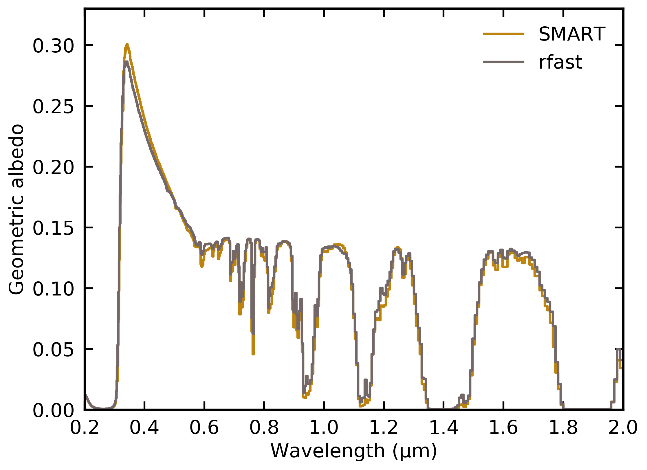
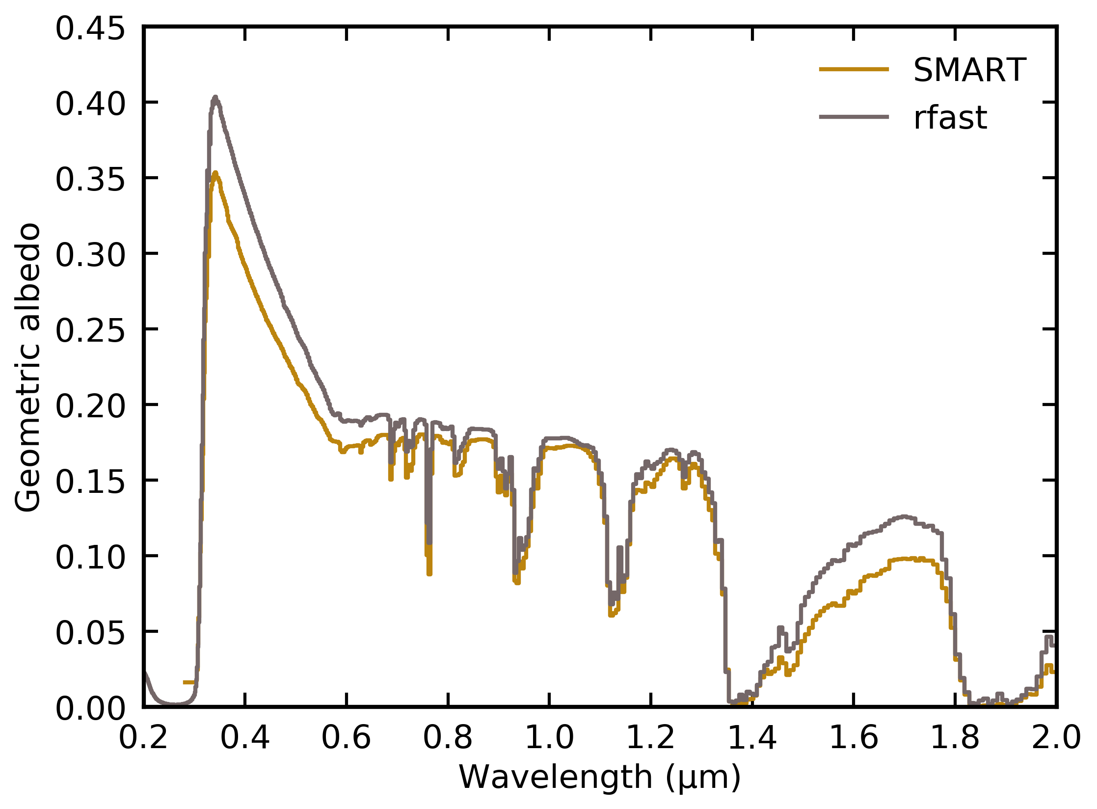
Figure 4: Reflection spectra for a partially-clouded (50% cloud coverage) Earth-like case from the rfast (grey) and SMART (yellow) models. Left figure is for a single-scene, plane-parallel setup. Right figure is for a three-dimensional treatment where plane-parallel calculations are run for pixels on the planetary disk and then spatially integrated.

Figures 5 and 6 show comparisons between rfast and SMART for clearsky thermal emission and transit spectroscopy cases, respectively. Thermal spectra are at a resolving power of 100 and show excellent agreement. Transit spectroscopy cases are also at a resolving power of 100 and plot effective transit altitude ($z_{\rm eff}$), which is defined by separating the solid-body contribution to a transit spectrum from the atmospheric component,

$$\left(\frac{R_{\rm p}+z_{\rm eff}}{R_{\rm s}}\right)^{\!\!2}=\left(\frac{R_{\rm{p},\lambda}}{R_{\rm{s}}}\right)^{\!\!2}\ .$$ (20)

The transit spectrum comparison shows scenarios that both include and exclude refraction effects for an Earth-Sun twin, where the scaTran addition to the SMART model incorporates refraction effects through ray tracing. A discrepancy (at less than one atmospheric pressure scale height) in the location of the transit floor for the rfast model arises as the incorporated analytic treatment of refraction can only be derived assuming an isothermal atmosphere. As the refractive bending is sensitive to atmospheric number densities, ray tracing through an atmosphere with a thermal structure profile yields a different (and more accurate) result than the analytic treatment. Fortunately, earlier modeling results show that refractive effects will be quite limited for the types of close-in exoplanets typically studied with transit spectroscopy (Bétrémieux & Kaltenegger, 2014; Misra et al., 2014; Bétrémieux & Swain, 2016; Robinson et al., 2017).

To summarize, the underlying radiative transfer routines within the rfast suite work well for transit applications (especially when refraction can be ignored), as the transmissivity calculations are in-line with more-sophisticated tools. Single-scene and thermal emission applications of rfast agree well with high-fidelity models, but biases can arise at levels typically less than 5–10%. Three-dimensional calculations of planetary reflectivity with rfast have larger disagreements when compared to high-fidelity models, and applications of the rfast inverse model to phase-dependent observations should be done with this limitation in mind. For comparison purposes, the high-fidelity, fully line-resolving, cloud-free column SMART simulations for single-scene reflectance, three-dimensional reflectance, thermal emission, and transit required single-core runtimes of 55 min, 430 min, 4.3 min, and 13.3 min, respectively, while the analogous rfast spectra required runtimes of 0.66 s, 6.8 s, 0.19 s, and 0.36 s, respectively. Thus, runtimes differ by a factor of 1,300–5,000.

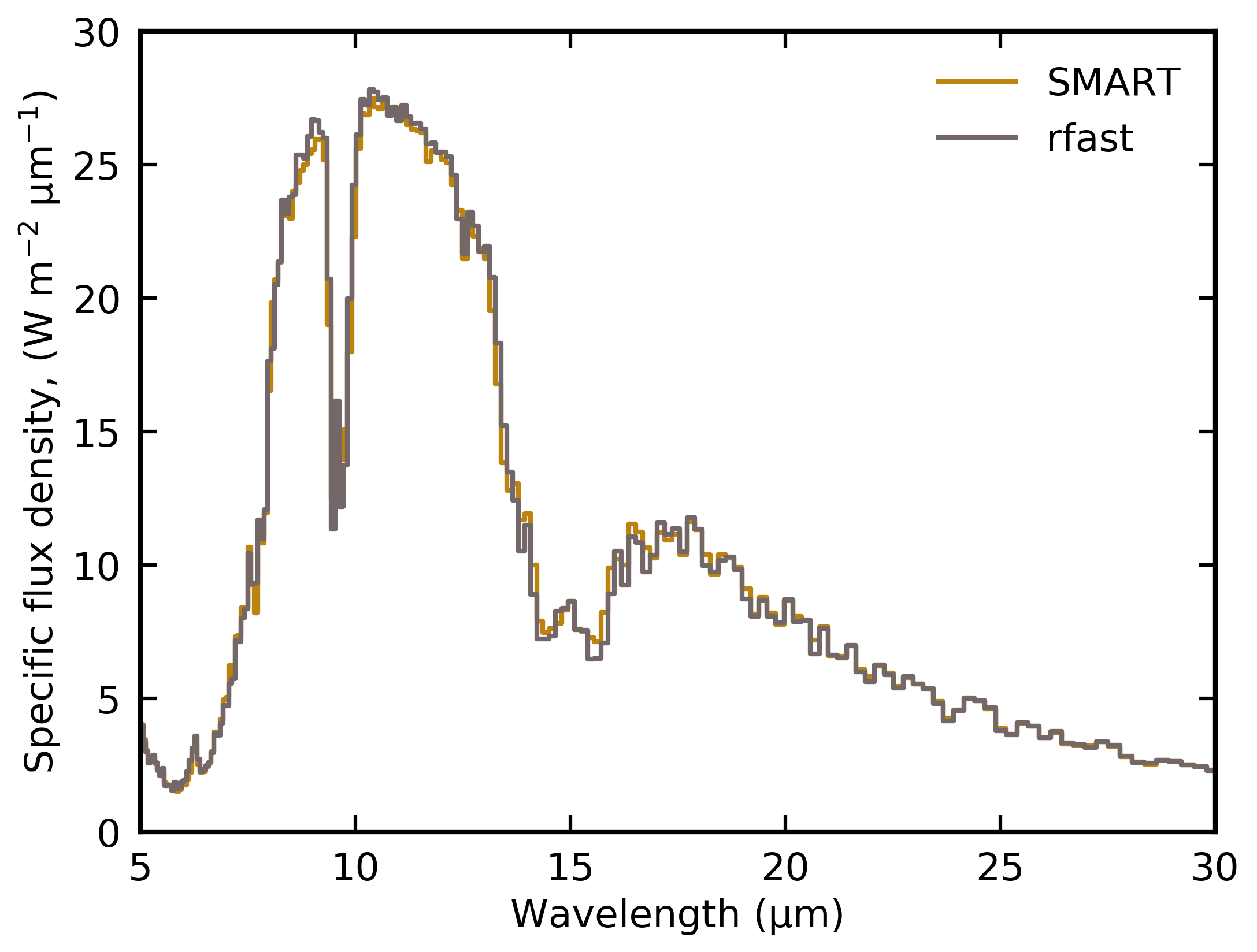
Figure 5: Thermal emission spectra for a clearsky Earth-like case from the rfast (grey) and SMART (yellow) models.

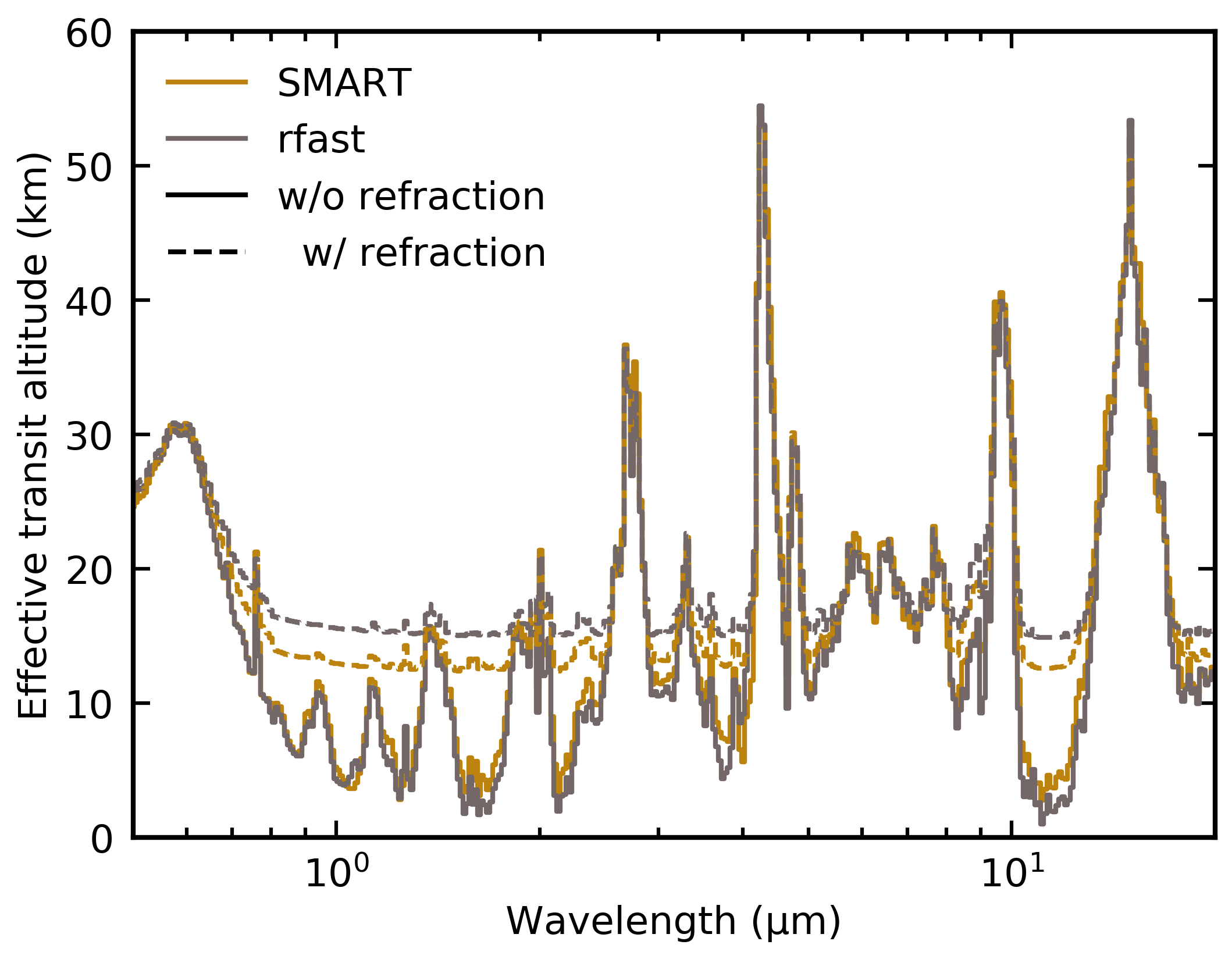
Figure 6: Transit spectra for a clearsky Earth-like case from the rfast (grey) and SMART (yellow) models. Scenarios that both include (dashed) and exclude (solid) refraction are shown.

3.3 Retrieval Validations

Feng et al. (2018) presented atmospheric retrieval results for simulated reflected light high contrast imaging observations of Earth-like exoplanets. Driven by initial ideas for the HabEx and LUVOIR concept missions, the Feng et al. (2018) results focused on visible wavelengths (0.4–1.0 $\upmu$m). Retrievals included 11 inferred parameters: planetary surface pressure ($p_{\rm s}$), planetary radius, planetary surface gravity, a grey surface albedo ($A_{\rm s}$), cloud top pressure ($p_{\rm c}$), cloud thickness (i.e., pressure extent; $\Delta p_{\rm c}$), cloud extinction optical depth ($\tau_{\rm c}$), cloud coverage fraction on the planetary disk ($f_{\rm c}$), and gas mixing ratios for water, ozone, and molecular oxygen ($f_{\rm H2O}$, $f_{\rm O3}$, and $f_{\rm O2}$, respectively; assumed to have constant vertical profiles). Except for planetary radius, all parameters were retrieved in log-space and molecular nitrogen was taken as the background gas. Uninformed priors were adopted for all parameters.

Figures 7 and 8 show retrieval results from the rfast tool that are analogous to a scenario in the Feng et al. (2018) work where the resolving power was fixed at 140 and the V-band SNR was taken as 20 (see simulated data with error bars in Figure 7). The simulated observations did not have uncertainties randomly applied to maintain consistency with Feng et al. (2018), who demonstrated that a statistical sampling of retrievals with randomized spectral errors yielded similar inference results to a case where errors are non-randomized and simply centered on the noise-free simulation. Note that the Feng et al. (2018) model is three-dimensional and uses 100 Gauss-Chebyshev integration points over the illuminated disk while the rfast retrieval was executed using the single-scene option. Figure 8 visualizes the full posterior distribution using the Python corner package (Foreman-Mackey, 2016) with one-dimensional marginal distributions for each parameter shown along the diagonal. Figure 7 shows forward model swaths at the 16–84 and 5–95 percentiles (i.e., 1- and 2-sigma for a Gaussian distribution).

For validation purposes, Table 1 compares inferred parameter values at the 16/50/84 percentiles from the Feng et al. (2018) study to those from rfast. Note that planetary radius was retrieved in log space with the rfast tool and then re-sampled to linear space for comparison to the Feng et al. (2018) results. Agreement between constraints is generally strong with 16–84 percentile spreads for nearly all cloud-unrelated parameters in rfast falling within 40% of the Feng et al. (2018) values, as indicated by the spread comparison column which differences the 16–84th percentile ranges from the two tools relative to the Feng et al. (2018) spread. Key exceptions occur for parameters related to clouds ($p_{\rm c}$, $\Delta p_{\rm c}$, $\tau_{\rm c}$, and $f_{\rm c}$) where rfast finds markedly weaker constraints. Detailed investigation reveals that the Feng et al. (2018) retrievals did not sufficiently progress Markov chain Monte Carlo simulations to map out the posterior distributions for poorly-constrained parameters — 100k walker steps are taken in the rfast retrieval versus 10k–20k for the Feng et al. (2018) retrievals. An equivalent test with the three-dimensional version of rfast further confirmed these results. Importantly, this comparison shows that, for low-SNR simulated data and retrievals related to mission concept studies, three-dimensional spectral models are likely not required for a first-order understanding of the mapping from predicted data quality to parameter constraints. When comparing the rfast tool to the Feng et al. (2018) model, this results in a runtime savings that scales with the number of disk integration points in the three-dimensional model.

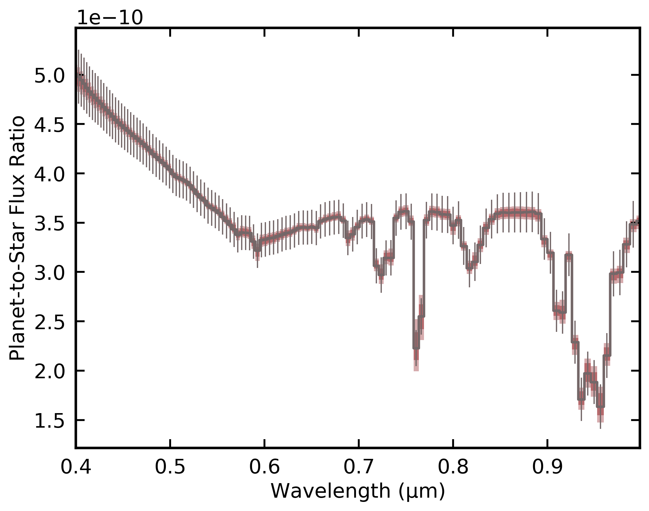
Figure 7: Simulated visible-wavelength reflected light observation of an exo-Earth at resolving power of 140 and a V-band SNR of 20 (points and associated error-bars, after Feng et al., 2018). Forward model spread from retrieval analysis as applied to the simulated observation is shown as darker and lighter swaths for 16–84 and 5–95 percentiles.

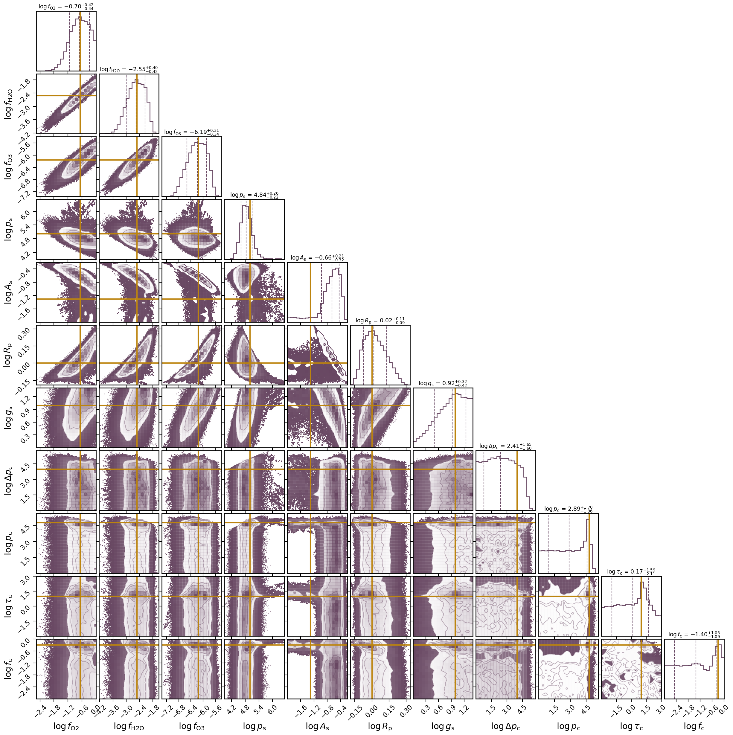
Figure 8: Visualized posterior distribution for eleven parameters from the rfast tool when retrieving on the simulated observations in Figure 7. One-dimensional marginal distributions are shown along the diagonal with associated 16/50/84-percentile values indicated above. Values used to generate the faux observation (i.e., “truth” values) are indicated as orange vertical and horizontal lines.

Table 1: Retrieval Model Comparison

Parameter	Units	Input	Feng+18	rfast	Spread Comparison
$\log p_{\rm s}$	log Pa	$5.0$	$5.07^{+0.39}_{-0.31}$	$4.84^{+0.26}_{-0.22}$	0.31
$R_{\rm p}$	$R_{\oplus}$	$1.0$	$1.05^{+0.42}_{-0.27}$	$1.04^{+0.20}_{-0.31}$	0.26
$\log g_{\rm s}$	log m s-2	$0.99$	$1.20^{+0.50}_{-0.64}$	$0.92^{+0.32}_{-0.42}$	0.35
$\log A_{\rm s}$		$-1.3$	$-0.79^{+0.34}_{-0.69}$	$-0.66^{+0.21}_{-0.32}$	0.49
$\log p_{\rm c}$	log Pa	$4.8$	$4.34^{+0.53}_{-0.85}$	$2.89^{+1.70}_{-1.96}$	1.65
$\log\Delta p_{\rm c}$	log Pa	$4.0$	$3.51^{+1.00}_{-0.98}$	$2.41^{+1.65}_{-1.60}$	0.64
$\log\tau_{\rm c}$		$1.0$	$0.79^{+0.87}_{-1.40}$	$0.17^{+1.59}_{-2.11}$	0.63
$\log f_{\rm c}$		$-0.3$	$-0.76^{+0.54}_{-1.26}$	$-1.40^{+1.05}_{-1.09}$	0.19
$\log f_{\rm H2O}$		$-2.5$	$-2.43^{+0.39}_{-0.56}$	$-2.55^{+0.40}_{-0.42}$	0.14
$\log f_{\rm O3}$		$-6.2$	$-6.03^{+0.34}_{-0.48}$	$-6.19^{+0.31}_{-0.34}$	0.21
$\log f_{\rm O2}$		$-0.68$	$-0.60^{+0.43}_{-0.59}$	$-0.70^{+0.42}_{-0.44}$	0.16

4 Results

In what follows, inferences from a variety of Solar System analog observations for exoplanets are explored using the rfast tool. Prior to these explorations, a demonstration application of the rfast tool is provided for a scenario near to its original design use — exoplanet direct imaging feasibility studies. Following this demonstration, the rfast tool is applied to reflected light observations of the distant Earth from NASA’s EPOXI mission (Livengood et al., 2011), providing a strong proof-of-concept for future exoplanet direct imaging missions. Next, retrieval analysis is used to understand information from a spacecraft-measured whole-disk infrared spectrum of Earth. Finally, an observationally-derived transit spectrum of Titan is studied using the rfast tool. As is common for exoplanet atmospheric retrievals, gas mixing ratios are assumed constant throughout the atmosphere (although the rfast tool can accommodate vertical structure in gas mixing ratios). The studies in this section are not intended to be exhaustive — myriad questions could be asked of these analog observations, likely motivating many stand-alone studies. Instead, the studies below are meant to be an example of how retrieval approaches can be understood and validated through application to worlds where detailed in situ (or orbiter/spacecraft) data exist. Finally, note that any detailed discussion of results derived in this section are reserved for Section 5.

4.1 Exo-Earth Reflected Light Direct Imaging

The rfast tool was originally designed to rapidly answer questions for development of exoplanet characterization-focused missions. As an example, Figure 9 shows a characteristic exo-Earth spectrum at resolving powers relevant to the HabEx and LUVOIR mission concepts (i.e., resolving powers of 7, 140, and 70 in the ultraviolet, optical, and near-infrared, respectively). Spectral impacts of species that are radiatively active in the depicted wavelength range are also indicated.

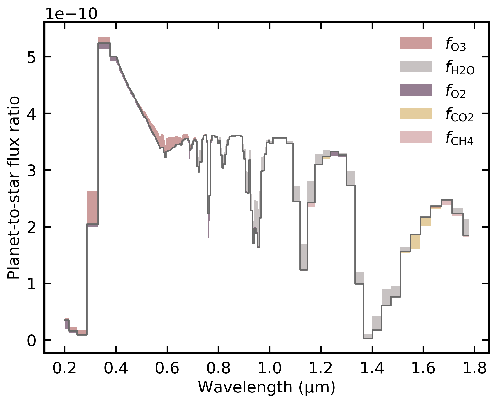
Figure 9: Simulated spectrum of an exo-Earth orbiting a solar twin at characteristic HabEx/LUVOIR spectral coverage and resolving power (ultraviolet [0.2–0.4 $\upmu$m], visible [0.4–1.0 $\upmu$m], and near-infrared [1.0–1.8 $\upmu$m] at resolving power of 7, 140, and 70, respectively). Gas spectral impacts are indicated by showing sensitivity to mixing ratio changes for key species. For the sensitivity test, and relative to fiducial values, the water vapor and ozone mixing ratios were halved, the molecular oxygen mixing ratios was doubled, and the carbon dioxide and methane mixing ratios were increased by a factor of 5.

Both the HabEx and LUVOIR mission concepts did not include capabilities to perform observations that simultaneously spanned the full ultraviolet through near-infrared range. Thus, extended spectral coverage could be traded for increased exposure time (and, thus, SNR) in a given band. Figure 10 demonstrates how gas constraints are impacted by spectral coverage and band SNR. For the underlying retrievals, the simulated observation was derived from the baseline spectrum in Figure 9, the rfast tool was run in its single-scene mode for reflected light, and the inferred parameters are the same 11 parameters as in Section 3.3 with the addition of mixing ratio inferences for CO₂ and CH₄: surface pressure ($p_{\rm s}$), planetary radius ($R_{\rm p}$), surface gravity ($g_{\rm s}$), grey surface albedo ($A_{\rm s}$), cloud-top pressure ($p_{\rm c}$), cloud pressure extent ($\Delta p_{\rm c}$), cloud optical depth ($\tau_{\rm c}$), cloud covering fraction ($f_{\rm c}$), and mixing ratios for water vapor, ozone, and molecular oxygen. One retrieval exercise was performed with the full spectral coverage (i.e., ultraviolet through near-infrared) and a V-band SNR of 20 (typical of what was proposed by the HabEx and LUVOIR concepts), another retrieval exercise used only the optical (0.4–1.0 $\upmu$m) range and a V-band SNR of 35, and a third retrieval exercise omitted the ultraviolet band, adopted a reduced optical SNR of 10, and used an enhanced near-infrared SNR of 45. The feasibility of these observing scenarios would depend on a number of parameters, including target distance and the presence of any systematic noise floors, and the rfast tool is designed to enable exploration of any such relevant observing scenarios. Future work could intercompare observing scenarios for different types of worlds using the rfast suite.

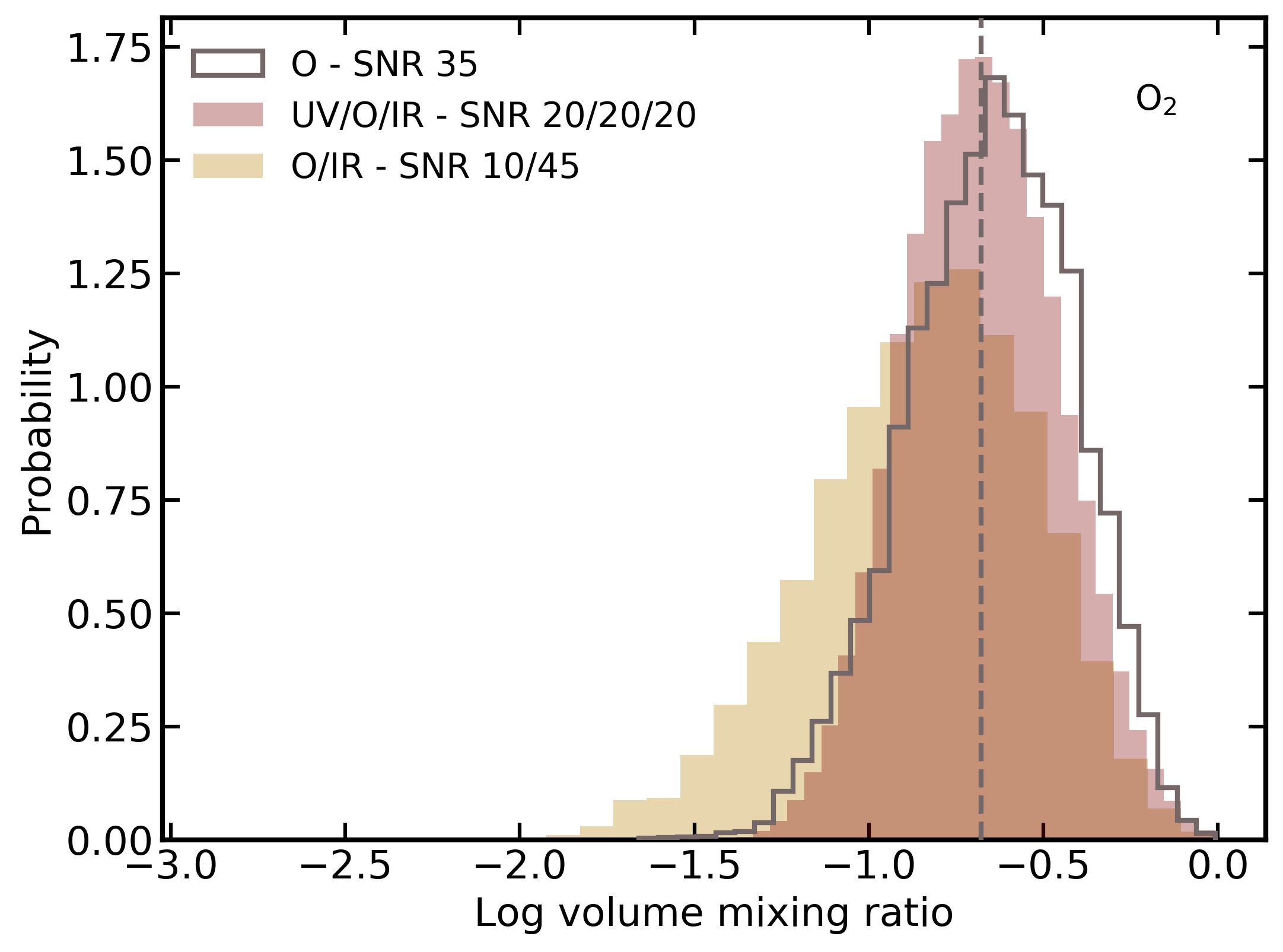
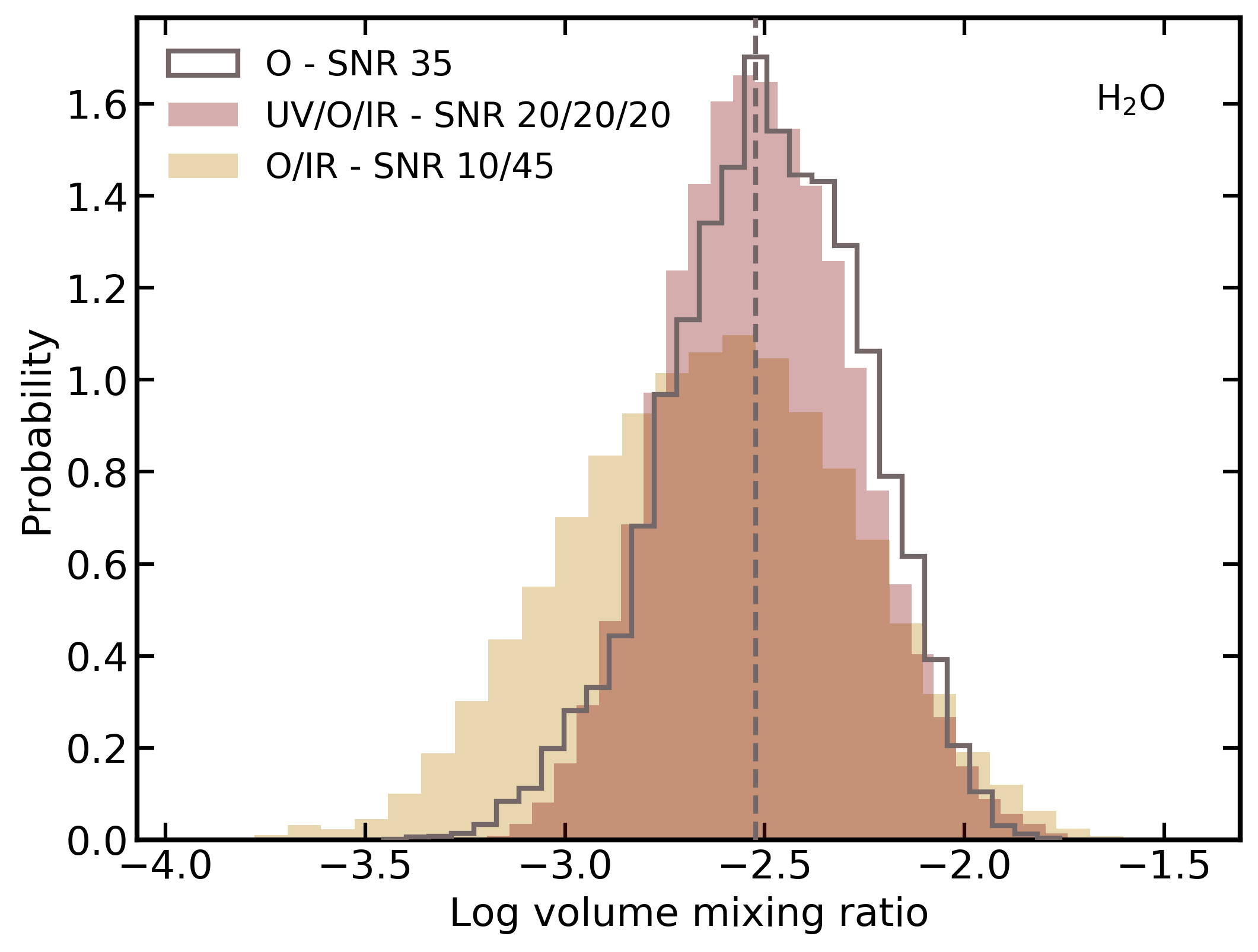
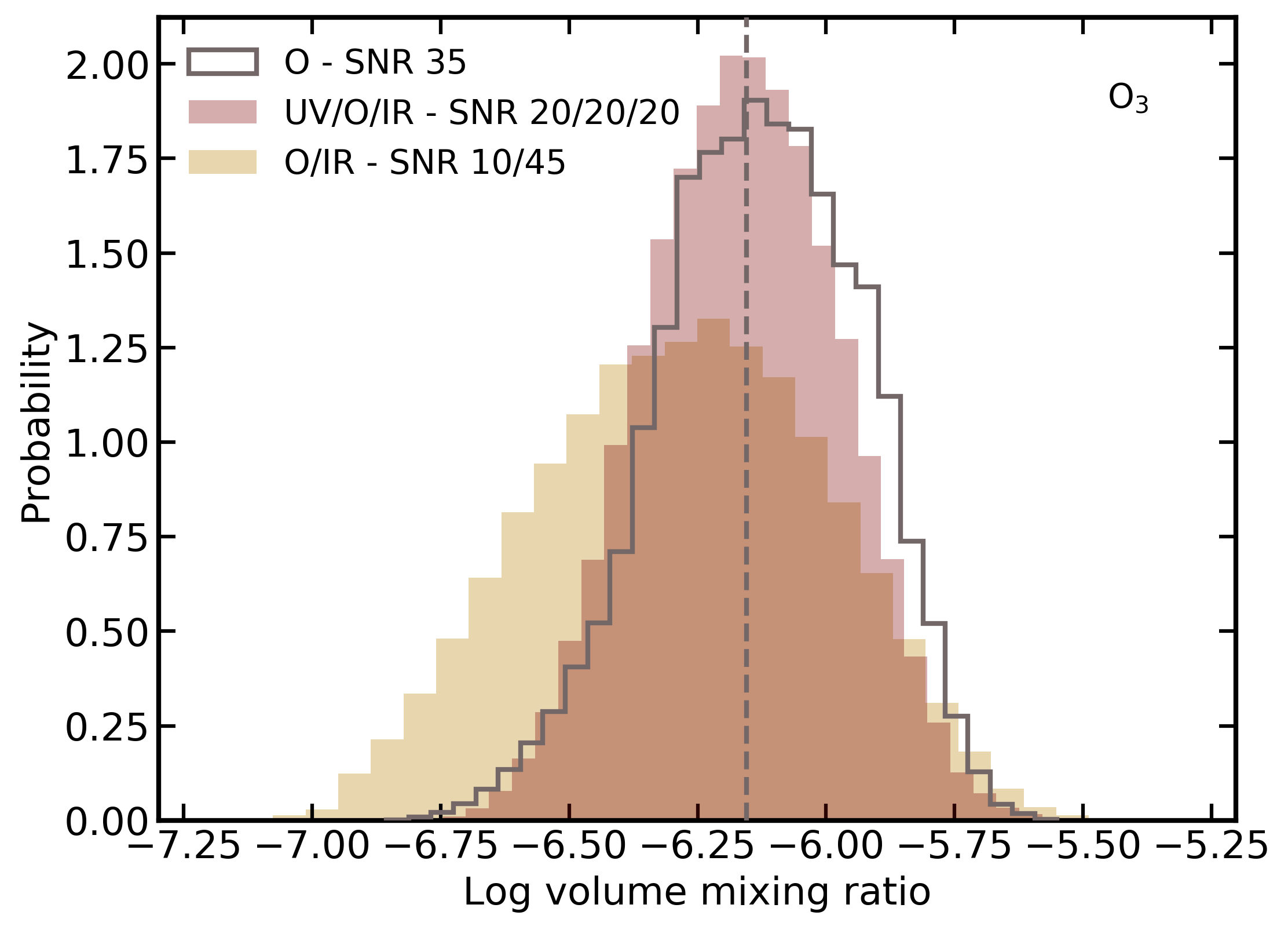
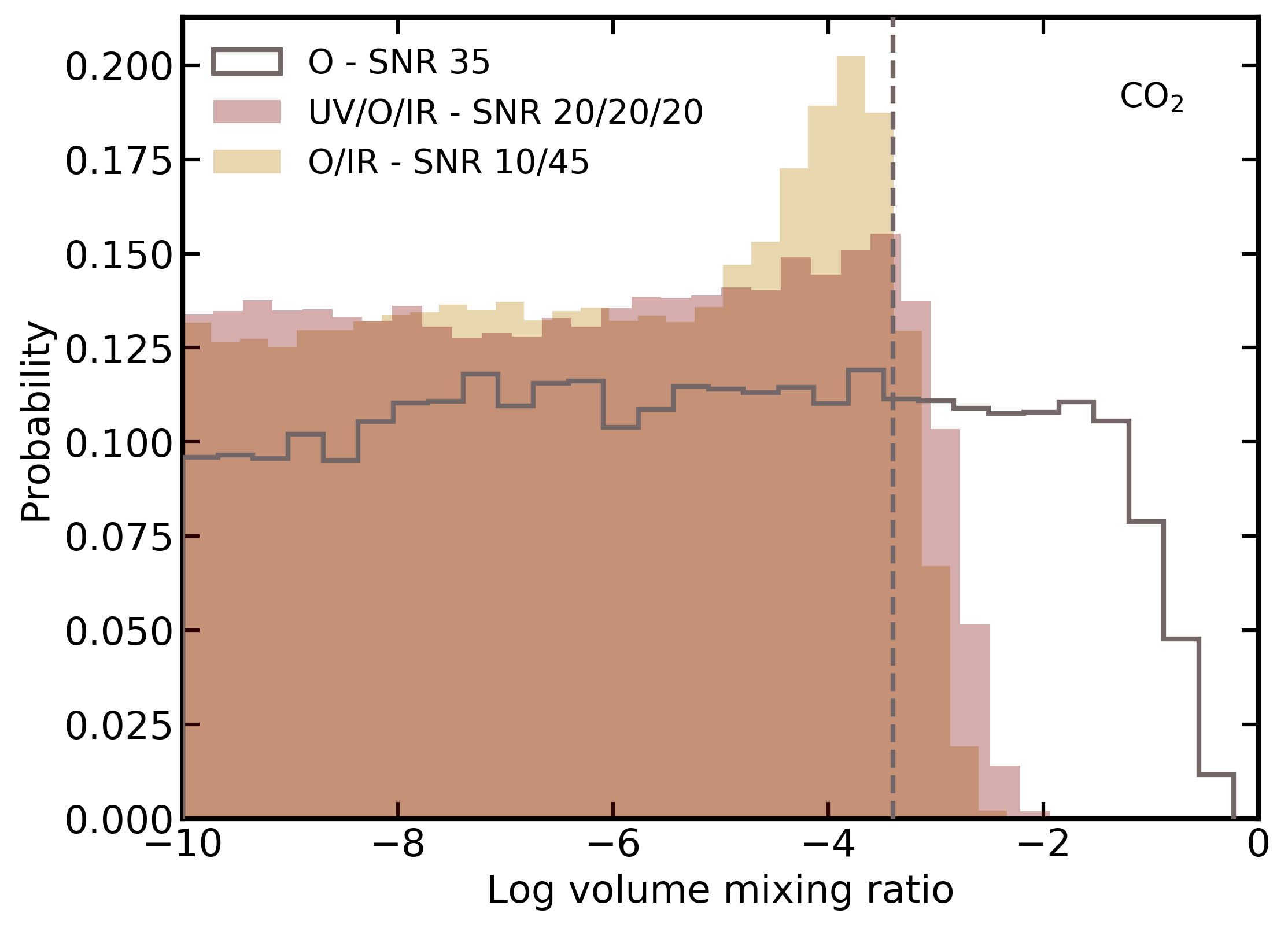
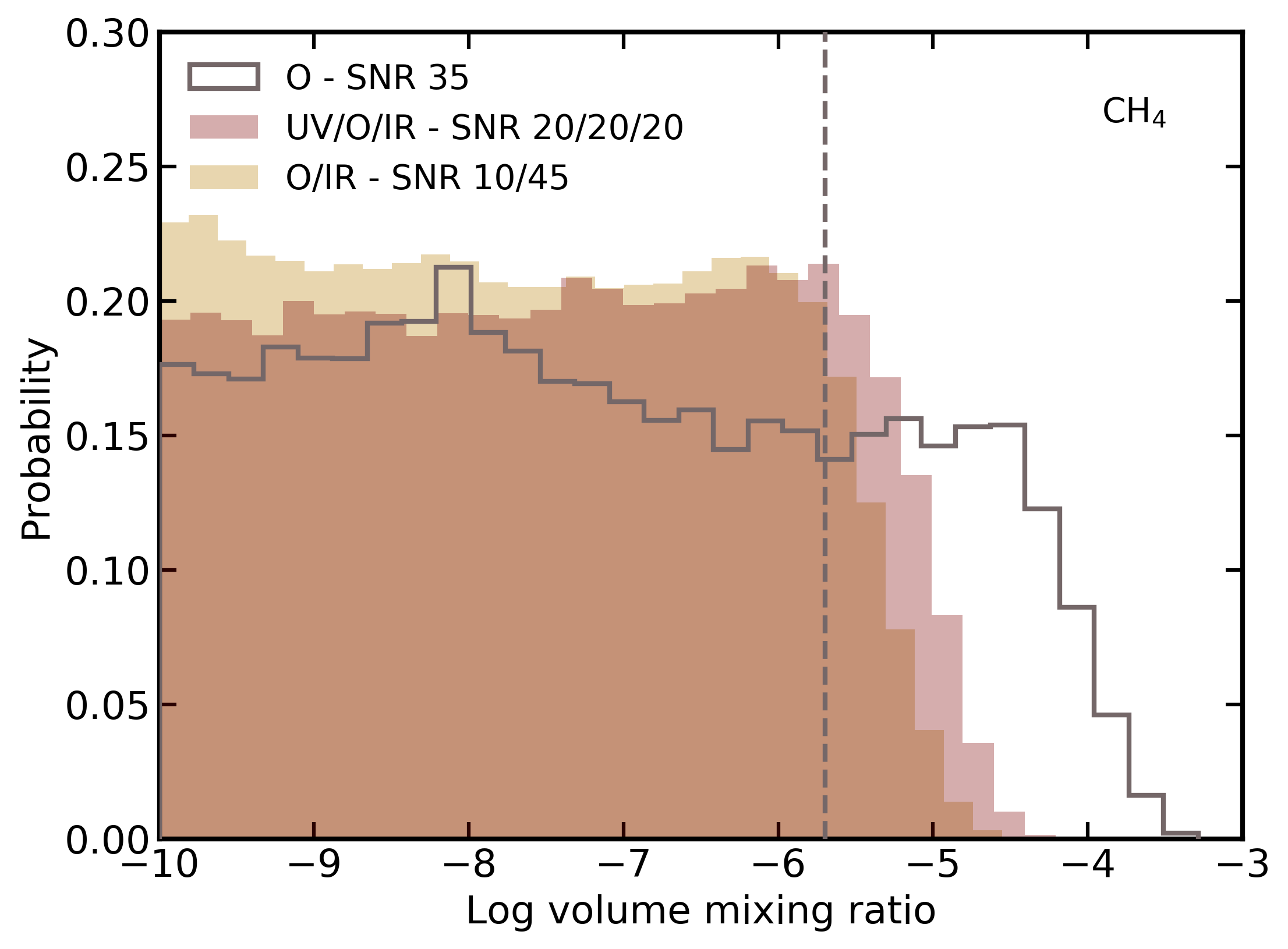
Figure 10: Constraints on key atmospheric species for three different HabEx/LUVOIR-like observing scenarios where spectral coverage and SNR are traded. One scenario has SNR of 20 across the ultraviolet, optical, and near-infrared bands, a second scenario has optical-only coverage at a enhanced SNR of 35, and a third has a reduced optical SNR of 10 and an enhanced near-infrared SNR of 45.

4.2 EPOXI Earth Retrievals

A repurposed application of NASA’s Deep Impact flyby spacecraft, dubbed the EPOXI mission, acquired whole-disk observations of Earth at distances of 0.18–0.34 au on three separate occasions in northern spring 2008 (Livengood et al., 2011). These data are important testing grounds for ideas related to exo-Earth atmospheric inference for HabEx- or LUVOIR-like concepts as the observations span ultraviolet through near-infrared wavelengths. Specifically, ultraviolet and visible wavelengths (0.37–0.95 $\upmu$m) are spanned by seven photometric bandpasses while near-infrared spectroscopy (1.1–4.54 $\upmu$m) is acquired at variable resolving power ($\lambda/\Delta\lambda$ of 215–730). For retrieval studies presented here, data from the 18–19 March observing sequence (at a phase angle of 57.7°) was rotationally averaged and trimmed to emphasize wavelengths plainly dominated by reflected light (i.e., data longward of 2.5 $\upmu$m were omitted). Additionally, data were scaled to full phase using a Lambertian phase function, which is an acceptable transformation for Earth at phase angles smaller than roughly 90° (Robinson et al., 2010). Trimmed and scaled data are shown in Figure 11 with uncertainties that are wavelength-independent and yield a SNR of 20 at V-band (i.e., characteristic of predicted HabEx and LUVOIR uncertainties for exo-Earth targets).

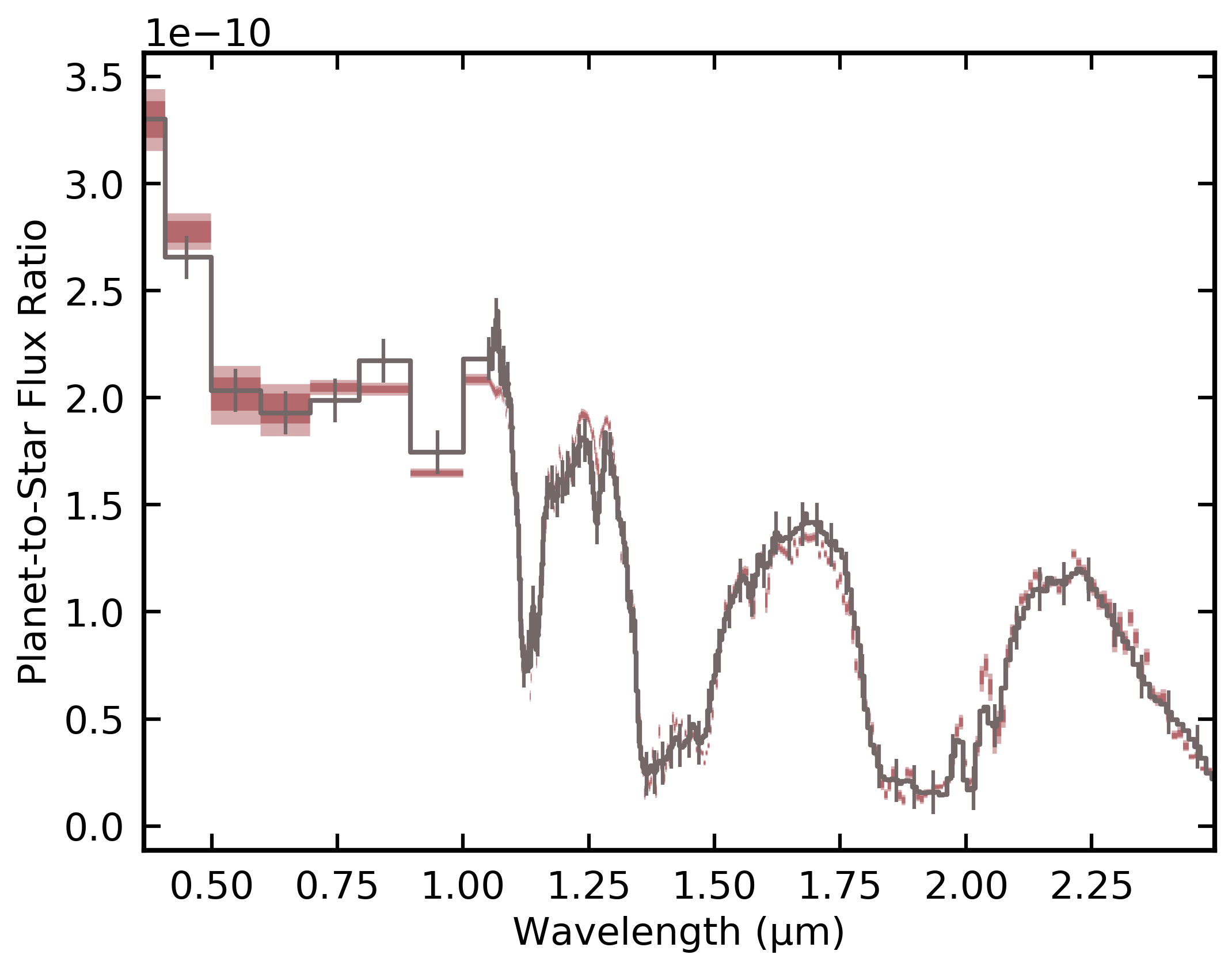
Figure 11: Photometric (below 1 $\upmu$m) and spectroscopic (above 1 $\upmu$m) reflected light observation of Earth from NASA’s EPOXI mission, rotationally averaged from the 18–19 Mar 2008 dataset (Livengood et al., 2011). Simulated wavelength-independent error bars yielding a V-band SNR of 20 are indicated, and only every fifth error bar is shown for spectroscopic data for clarity. Forward model spread from retrieval analysis is shown as darker and lighter swaths for 16–84 and 5–95 percentiles.

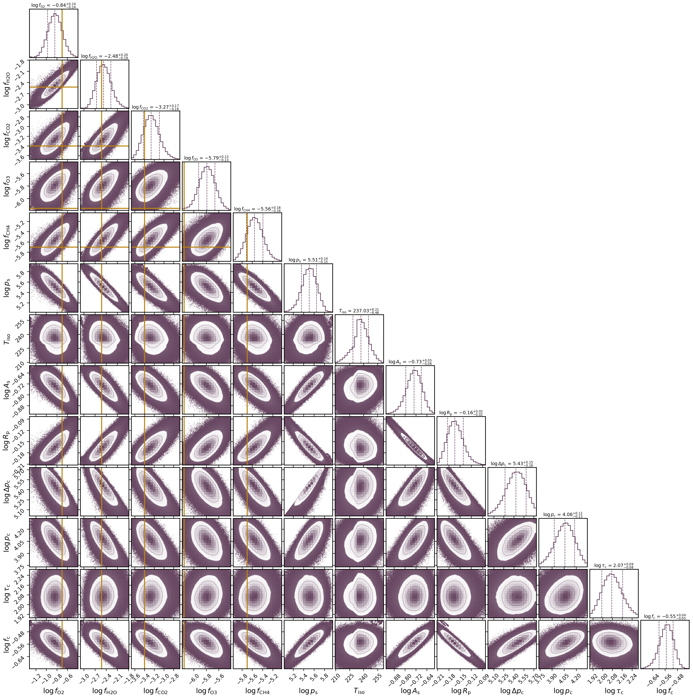
Figure 20: Visualized posterior distribution for a 13-parameters fit to the SNR of 20 EPOXI Earth observations in Figure 11. One-dimensional marginal distributions are shown along the diagonal with associated 16/50/84-percentile values indicated above and with vertical dashed lines. When relevant a priori values are well-known, a vertical line indicates the characteristic “truth” value for Earth.

Retrievals were performed on the EPOXI data shown in Figure 11 using the rfast single scene reflected light mode. Thirteen (13) parameters are retrieved: the volume mixing ratios for O₂, H₂O, CO₂, O₃, and CH₄, as well as surface pressure ($p_{\rm s}$), an isothermal atmospheric temperature ($T_{\rm iso}$), a grey surface albedo ($A_{\rm s}$), planetary radius ($R_{\rm p}$), cloud pressure extent ($\Delta p_{\rm c}$), top-of-cloud pressure ($p_{\rm c}$), cloud optical thickness ($\tau_{\rm c}$), and cloud coverage fraction ($f_{\rm c}$). Blended water liquid/ice optical properties were assumed for cloud asymmetry parameter and single scattering albedo. Planetary mass was fixed at $1\,M_{\oplus}$, as could be the case for an exo-Earth with a mass constraint from radial velocity data. Figure 20 (in Appendix) shows constraints from analyzing the EPOXI spectrum at a SNR of 20, which are generally comparable to those from the SNR of 20 experiment in Section 4.1. Notable differences include that both carbon dioxide and methane are confidently inferred in the EPOXI retrievals, stemming from the presence of relatively strong carbon dioxide and methane features in the 1.8–2.5 $\upmu$m range. Cloud fraction is constrained at roughly 30% from the EPOXI data and cases with opaque clouds that extend through the deep atmosphere with a cloud top pressure near the tropopause are preferred.

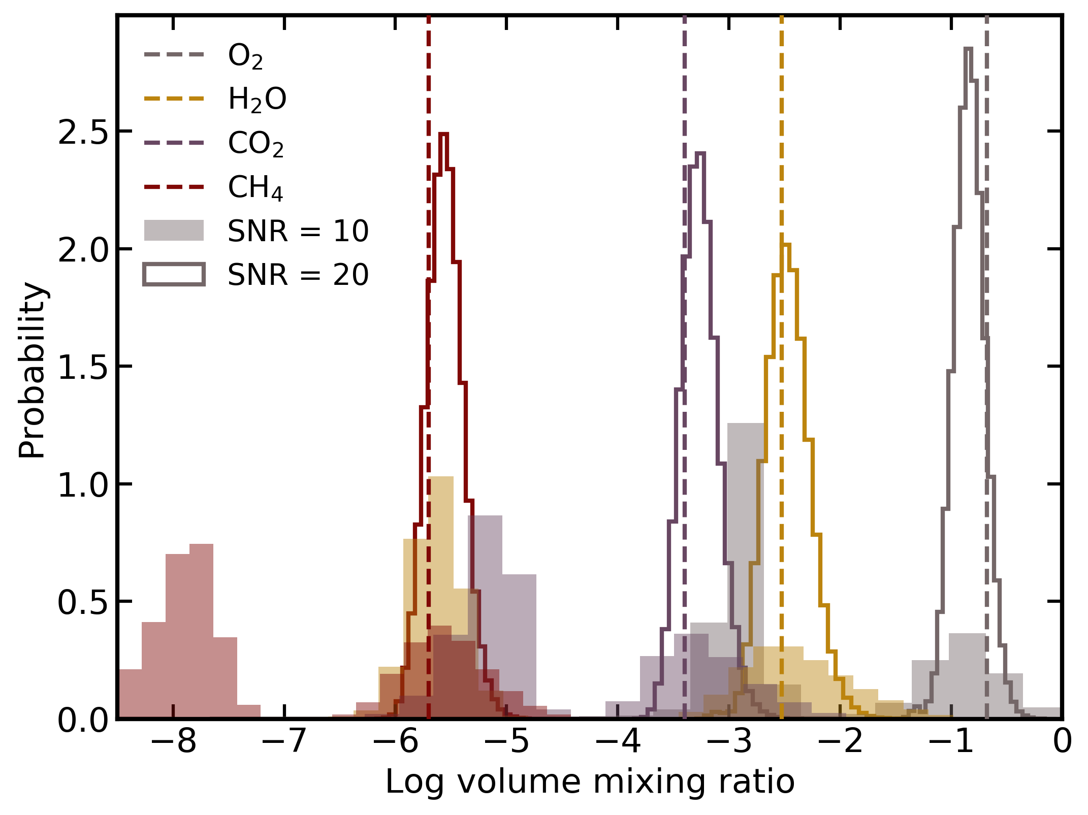
Figure 12: Gas mixing ratio constraints from retrievals performed on EPOXI observations of Earth degraded to V-band SNR of 10 (filled) and 20 (unfilled). Gases are represented with different colors and vertical lines indicate known “truth” values. At SNR of 10, gas posteriors include a peak near a realistic value and a second, unrealistic peak due to an inability to rule out solutions with a deep atmosphere.

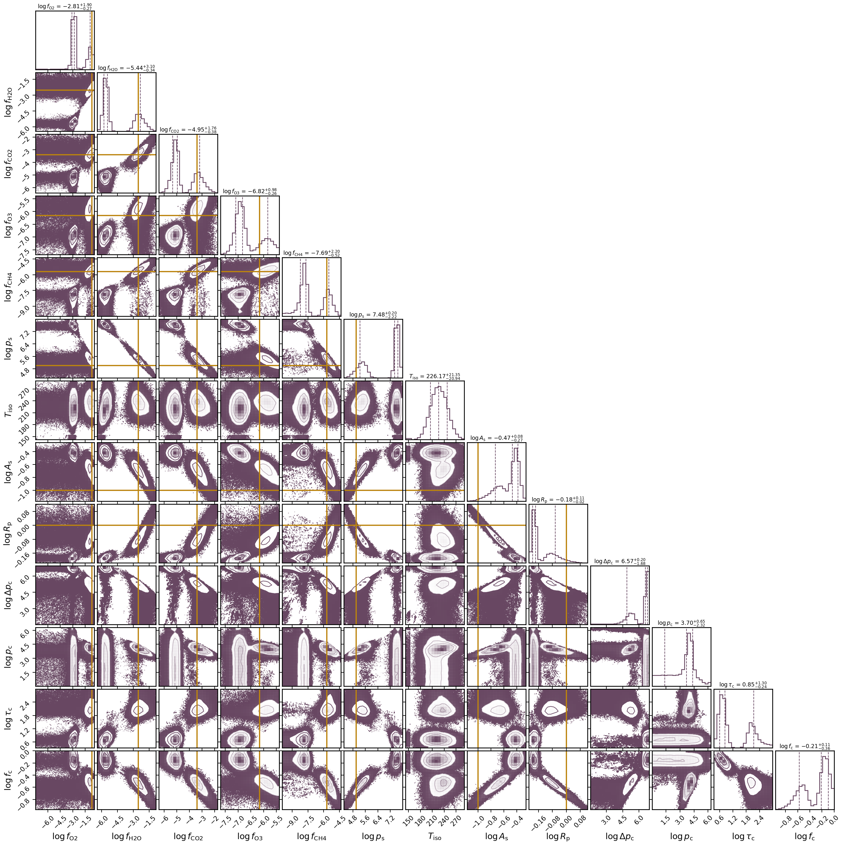
Figure 21: Same as Figure 20 except that the underlying EPOXI Earth observations have been degraded to a V-band SNR of 10.

An additional experiment was run retrieving on the EPOXI data where the wavelength-independent noise was then set to yield a SNR of 10 in V-band. Results are shown in Figure 21 (in Appendix). Comparing the inferences from the SNR of 20 scenario to those from the SNR of 10 scenario provides insight into how constraints on atmospheric and planetary parameters degrade with decreasing SNR. Unsurprisingly, broader ranges of parameters (i.e., poorer constraints) are found to be consistent with the SNR of 10 EPOXI data. More specifically, two distinct categories of atmospheric states are inferred as providing acceptable fits — an atmospheric state that is similar to the solutions found in the SNR of 20 experiment as well as an atmospheric model that has (1) near-total coverage of extended, diffuse clouds, (2) a deep atmosphere/surface boundary (i.e., large $p_{\rm s}$), and (3) gas mixing ratios that are reduced by orders of magnitude (to maintain roughly fixed column number density at these larger pressures). Figure 12 demonstrates the impact on gas mixing ratio constraints as the SNR is degraded from 20 to 10, and Figure 13 shows the correlation between “surface” pressure and cloud fraction for the SNR of 10 scenario where an unrealistic set of solutions with an effectively infinitely deep atmosphere cannot be ruled out. In such a case, additional prior information or longer exposure times would be required to better-refine constraints on the atmospheric state.

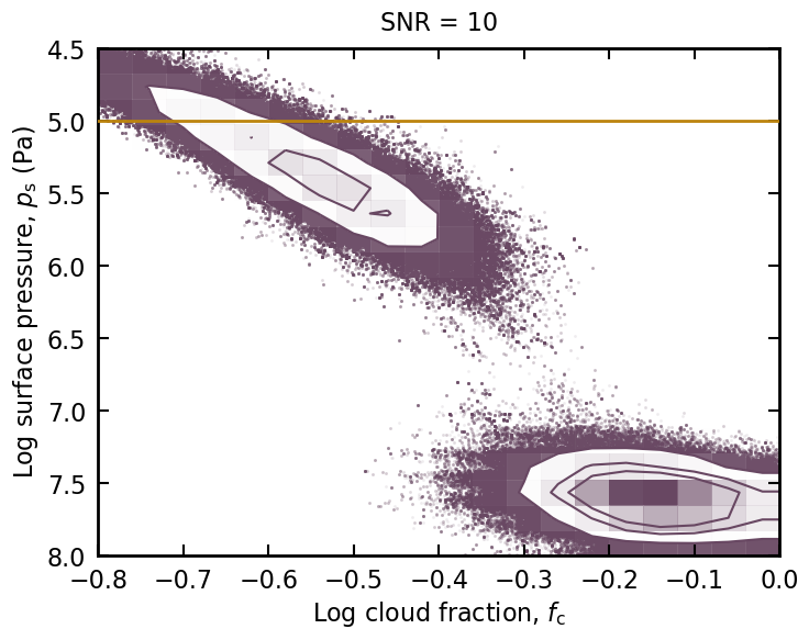
Figure 13: Correlation between inferred cloud coverage fraction and surface pressure for retrievals performed on EPOXI data at SNR of 10. Two classes of solutions emerge: one with realistic surface pressures (horizontal line) and cloud coverages and another with a deep atmosphere and near-global coverage of modest-thickness clouds.

4.3 Earth Infrared Retrievals

The Mars Global Surveyor Thermal Emission Spectrometer (MGS-TES) captured a full-disk infrared spectrum of Earth on November 24, 1996, from a distance of $4.8\times 10^{6}$ km (0.032 au) (Christensen & Pearl, 1997). The observing sequence was centered over the Pacific ocean at 18° N and 152° W, and spanned 6–50 $\upmu$m at a constant resolution of 10 cm^-1 (i.e., spanning resolving powers of 160–14 from the shortest to longest wavelengths). For retrieval studies presented here, data shortward of 7 $\upmu$m and longward of 40 $\upmu$m are omitted; flux densities at the shortest wavelengths are anomalously large (see Figure 10 of Robinson & Reinhard, 2020) (which strongly biased early retrieval studies explored for this work) and brightness temperatures at the longest wavelengths are unphysically large (i.e., exceeding 1,000 K). The truncated spectrum is shown in Figure 14 where wavelength-independent uncertainties have been added to yield a SNR of 20 at 10 $\upmu$m. Thus, adopted data quality is roughly consistent with under-study mid-infrared exo-Earth direct imaging mission concepts (Quanz et al., 2021a), where studies have investigated wavelength coverage of 3–20 $\upmu$m, resolving powers of 20–100, and SNRs of 5–20 (Konrad et al., 2021).

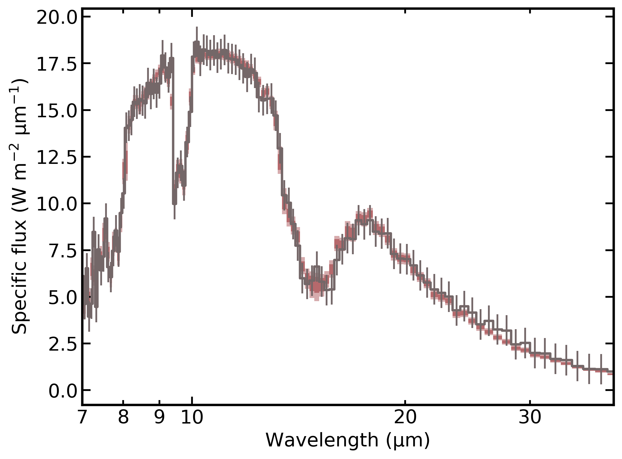
Figure 14: Earth thermal infrared spectrum from MGS-TES (Christensen & Pearl, 1997) trimmed to 7–40 $\upmu$m, as described in text. Adopted error bars are constant in wavelength and yield SNR of 20 at 10 $\upmu$m. Forward model spread from retrieval analysis is shown as darker and lighter swaths for 16–84 and 5–95 percentiles.

A retrieval was performed on the data (with faux uncertainties) shown in Figure 14 using the rfast tool. Twelve (12) parameters were inferred, including: surface pressure ($p_{\rm s}$), planetary radius ($R_{\rm p}$), cloud fraction ($f_{\rm c}$), cloud-top pressure ($p_{\rm c}$), and the volume mixing ratios for water vapor, carbon dioxide, ozone, nitrous oxide, and methane. Planetary mass (or, equivalently, surface gravity) was assumed to be well-known, as would be the case, e.g., if prior precision radial velocity data were available (recent, analogous retrieval results have shown that spectral inference does not serve to improve mass estimates beyond a mass prior; Alei et al., 2022). Additionally, to maintain a simple model for clouds, the cloud pressure extent was taken as a single scale height. Finally, a baseline model assumes a thermal structure that follows a power-law from the surface through the “troposphere,” with,

$$T\left(p\right)=T_{\rm s}\left(\frac{p}{p_{\rm s}}\right)^{\beta_{\rm t}}\ ,$$ (21)

where the surface temperature, $T_{\rm s}$, and $p$-$T$ power-law index, $\beta_{\rm t}$, are fitted parameters. The “stratosphere” was taken as isothermal at a temperature $T_{\rm iso}$, which was also fitted. All priors were uninformed.

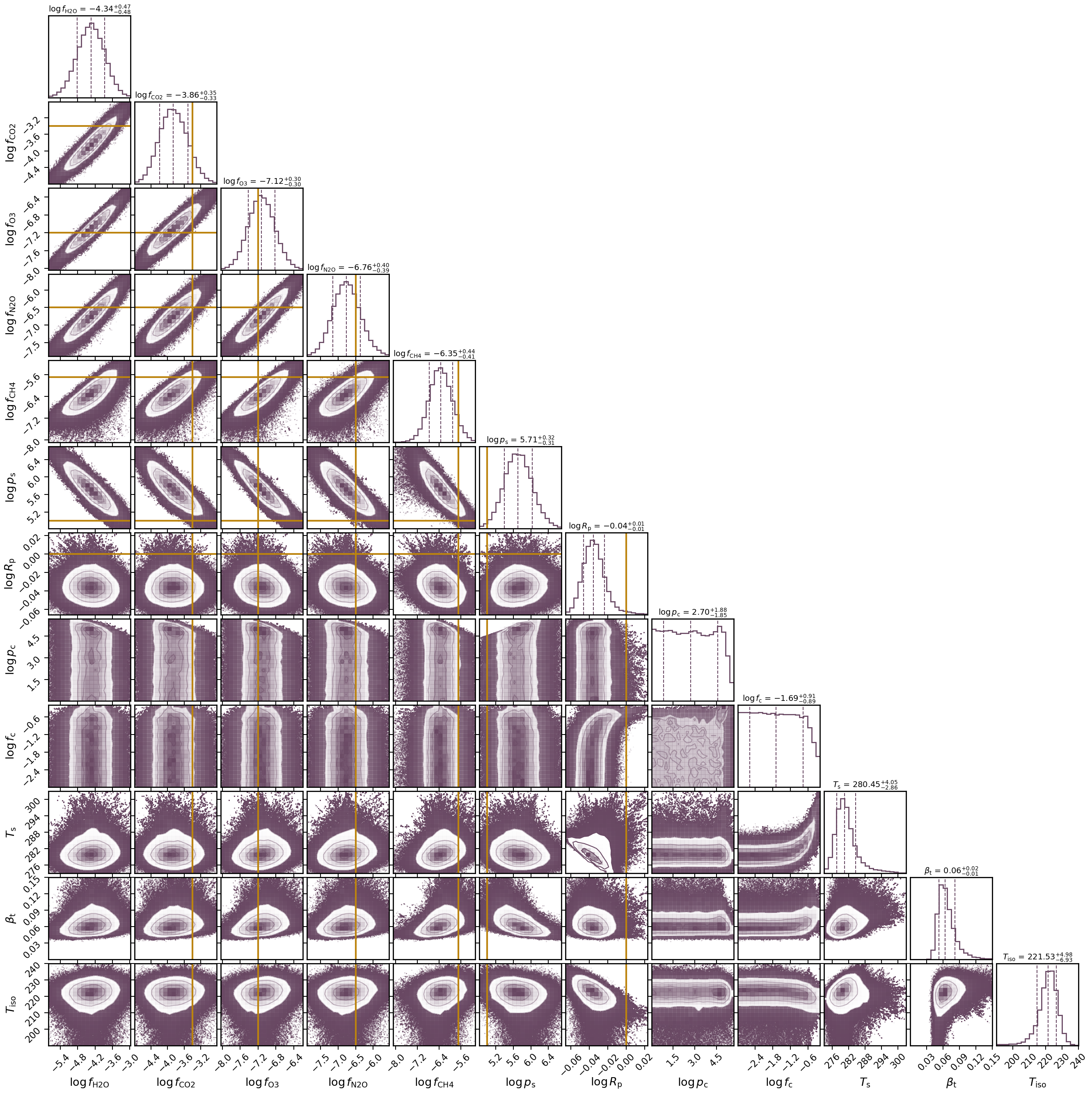
Figure 22: Visualized posterior distribution for a 12-parameters fit to the MGS-TES Earth observations in Figure 14. One-dimensional marginal distributions are shown along the diagonal with associated 16/50/84-percentile values indicated above and with the vertical dashed lines.

Figure 22 (in Appendix) shows retrieval results for the 12-dimensional fit to the MGS-TES observations. As shown in Figure 15, gas mixing ratios are well-constrained and generally reasonable — characteristic values for the log of volume mixing ratios for carbon dioxide, nitrous oxide, and methane (in 1996) are -3.4, -6.5, and -5.7, respectively. Ozone mixing ratios in the deep atmosphere — as is mainly probed by the 9.6 $\upmu$m ozone feature — span -7.3 to -6.3 (in log space). The inferred water vapor volume mixing ratio distribution (with characteristic values below about 0.01%) appears to be biased low, potentially pointing to remaining systematic issues affecting the 6.3 $\upmu$m water vapor band. Surface pressures are biased high by roughly a factor of $5$ and the planetary radius constraint — which would be strong by most exoplanet standards — is biased towards smaller radii (by about 10%). Cloud-top pressure is largely unconstrained and only near-total cloud coverage fractions are ruled out. The inferred surface temperature is generally above the water freezing temperature, and preferred thermal structures have decreasing temperatures with pressures. Figure 14 shows spectral forward model swaths at the 16–84 and 5–95 percentiles.

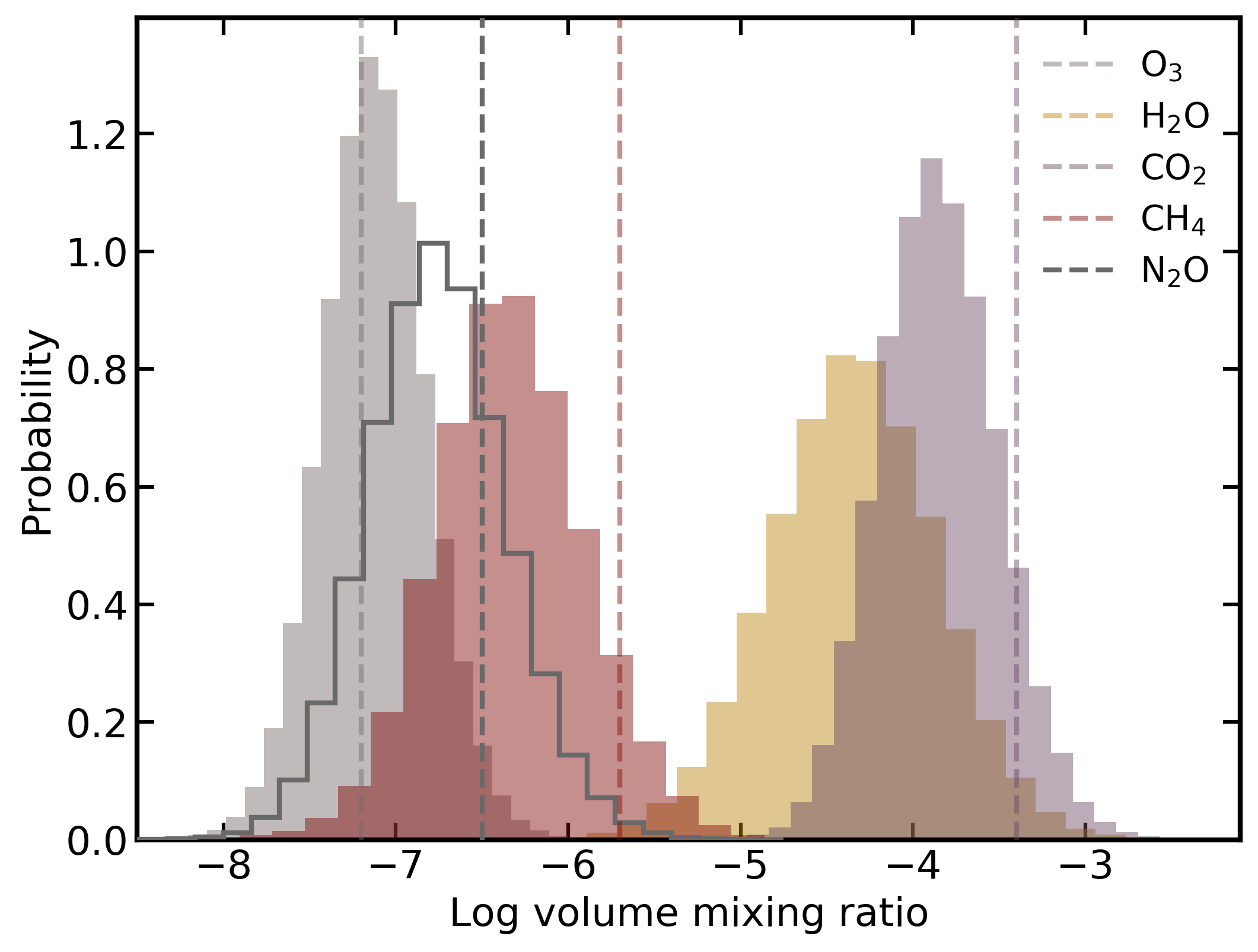
Figure 15: Gas mixing ratio constraints from retrievals performed on the MGS/TES observations of Earth shown in Figure 14. Gases are represented with different colors and vertical lines indicate known “truth” values.

Figure 16 shows a two-dimensional histogram of inferred thermal structures for the 12-dimensional fit (and its three-parameter thermal structure model). Characteristic Earth thermal structure profiles (tropical and mid-latitudes) from McClatchey et al. (1972) are also shown. Model isothermal stratospheres show a strong preference for values near 220 K, and agreement with realistic Earth $p$-$T$ data is acceptable through the upper troposphere. However, retrieved thermal structures generally have a less-steep $p$-$T$ relation through the troposphere (as compared to the Earth data) and extend to higher pressures (stemming from the biased-high surface pressure constraint). To explore a more realistic thermal structures — and given that the largest data-model discrepancies in Figure 14 occur in the core of the 15 $\upmu$m carbon dioxide band (which is sensitive to a thermal inversion in the stratosphere of Earth) — a second retrieval was performed with a thermal structure model that introduced a stratospheric $p$-$T$ power law, thereby allowing for thermal inversions. Thermal structures from this 13-dimensional fit are shown in Figure 16, which demonstrates only weak constraints on a stratospheric inversion. Reduced chi-squared values for the 12-dimensional and 13-dimensional fits are nearly identical (0.72 versus 0.71, respectively), which disfavors the model with an added treatment for stratospheric inversions.

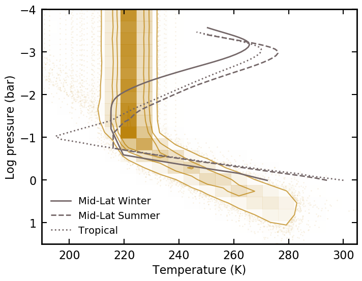
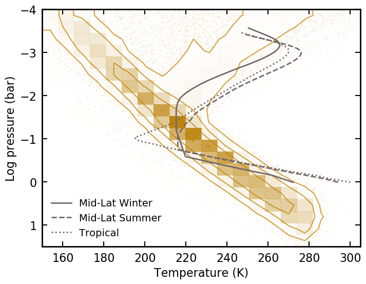
Figure 16: Two-dimensional histograms of thermal structure models randomly selected from retrievals on MGS-TES Earth observations. Standard Earth thermal structures from McClatchey et al. (1972) are shown as grey lines. Left figure is from a retrieval with a three-parameters thermal structure model (power-law troposphere profile and isothermal stratosphere) while right figure is from a retrieval with a four-parameters thermal structure model (power laws in both the troposphere and stratosphere).

4.4 Titan Transit Retrievals

The Visual and Infrared Mapping Spectrometer (VIMS; Brown et al., 2004) aboard NASA’s Cassini mission observed many solar occultations by Titan (Bellucci et al., 2009; Hayne et al., 2014; Maltagliati et al., 2015), and these can be translated into effective transit spectra (Robinson et al., 2014). Figure 17 shows a Titan transit spectrum derived from an occultation observation at 27° N, which was observed in September of 2011 and is an intermediate haze-extinction case provided by Robinson et al. (2014). Data span 0.88–5 $\upmu$m and resolution increases with wavelength from 12 nm to 18 nm. Refractive loss effects were removed from the underlying occultation data (following Robinson et al., 2014) so that fits to the resulting Titan transit spectrum need not consider refraction.

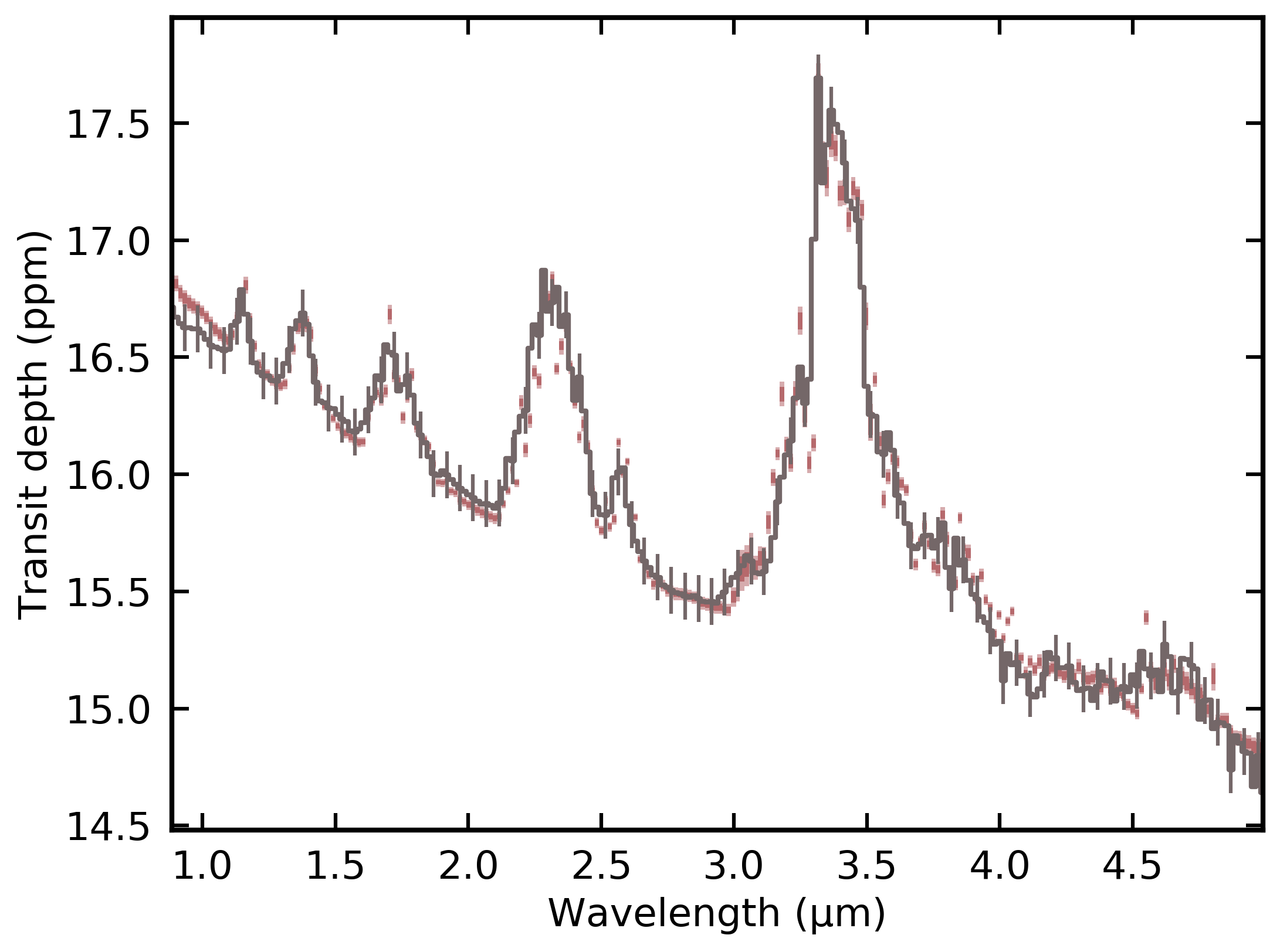
Figure 17: Titan transit spectrum derived from Cassini-VIMS observations (from Robinson et al., 2014). Adopted error bars are 0.1 ppm and are constant with wavelength, as justified in the text. Forward model spread from retrieval analysis is shown as darker and lighter swaths for 16–84 and 5–95 percentiles.

The rfast model was used to perform atmospheric retrievals on the transit spectrum shown in Figure 17. Faux error bars were assigned at the level of 0.1 ppm, which results in a ratio of error bar size to spectral feature depth that is roughly comparable to those from JWST-relevant clearsky, solar metallicity, warm Neptune cases investigated by Greene et al. (2016). Based on previous work analyzing VIMS Titan occultation data (Maltagliati et al., 2015; Cours et al., 2020), fits included volume mixing ratios for carbon monoxide, methane, acetylene (C₂H₂), and propane (C₃H₈). The fitted planetary radius was applied at the 10 mbar pressure level (Benneke & Seager, 2012). The spectral impact of haze was incorporated using a three-parameter model with (1) the vertical optical depth following an exponential with scale height, $H_{\rm h}$, (2) the wavelength-dependent opacity following a power law in wavelength with exponent $\beta_{\rm h}$, and (3) the optical depth at a wavelength of 1 $\upmu$m and at 10 mbar atmospheric pressure given by $\tau_{\rm h}$. To capture the known strong decrease in temperature from Titan’s stratosphere to a cold tropopause, a three-parameter temperature model was adopted that follows,

$$T\left(p\right)=\left(T_{\rm{st}}-T_{0}\right)e^{-\frac{p}{p_{\rm T}}}+T_{0}\,$$ (22)

where $T_{\rm{st}}$ represents the hot stratopause temperature, $T_{0}$ represents a cold deep-atmosphere temperature, and $p_{\rm T}$ is the pressure scale for the decrease in stratospheric temperatures.

Initial retrievals resulted in inferred values for $\beta_{\rm h}$ that were much smaller than previously-derived results (Hubbard et al., 1993; Tomasko et al., 2008; Bellucci et al., 2009; Robinson et al., 2014). Closer investigations revealed that these errant power values were driven by attempts to use haze opacity to fit continuum near 4.3 $\upmu$m. Experiments revealed that this continuum could be better reproduced by including N₂-N₂ collision-induced absorption, so the nitrogen volume mixing ratio was added as a fitted parameter.

Several previous works have highlighted the role of a 3.4 $\upmu$m C-H stretch feature in Titan occultation observations (Maltagliati et al., 2015; Robinson et al., 2014; Cours et al., 2020). Optical depth data from interstellar medium observations were adopted to model the shape of this stretch feature (Pendleton & Allamandola, 2002). As the feature tracks condensed-phase hydrocarbons, the stretch feature optical depths were fitted by scaling the 1 $\upmu$m haze optical depths by a factor $x_{\rm C-H}$, and multiplying by the interstellar medium optical depths to capture the wavelength-dependent feature shape.

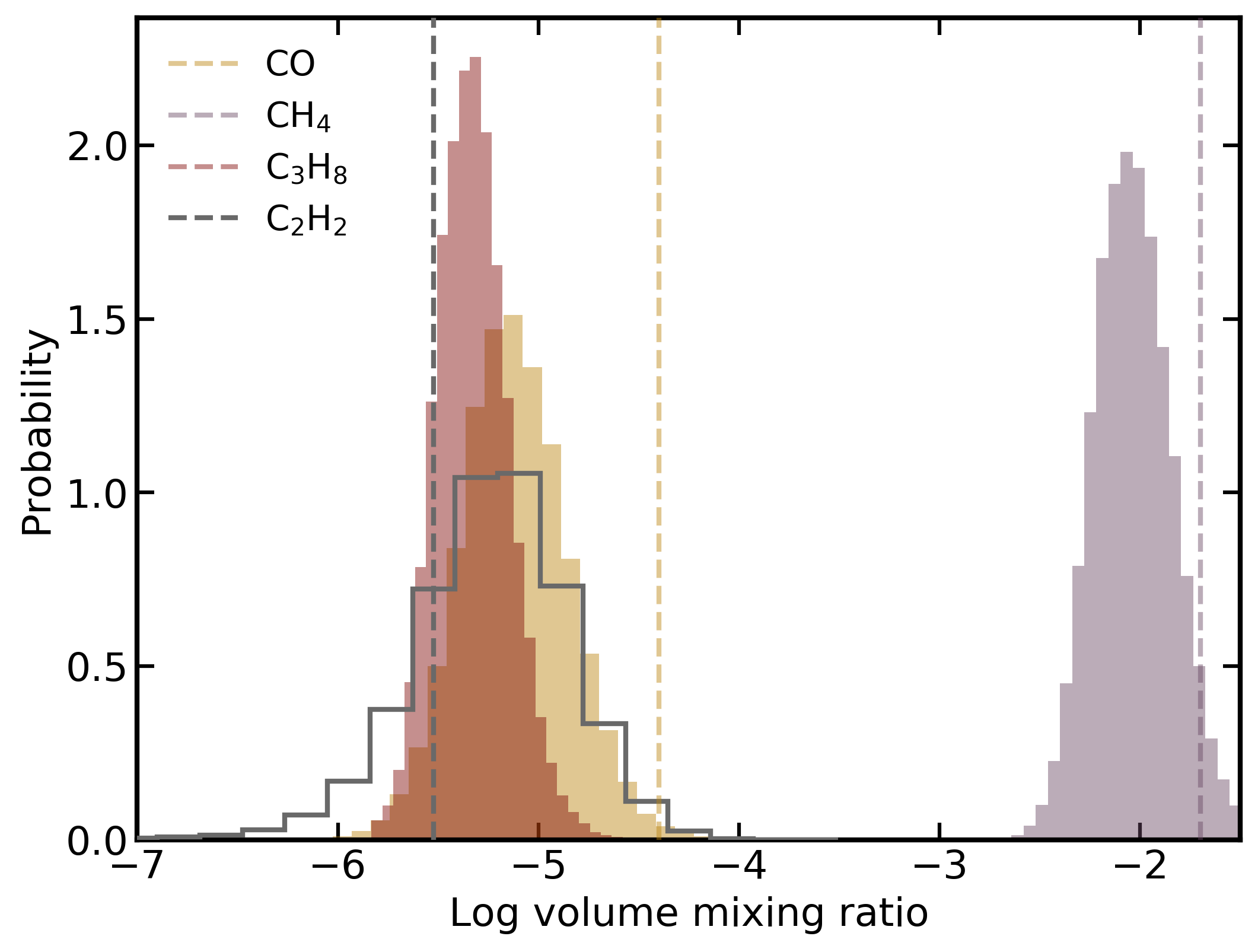
Figure 18: Gas mixing ratio constraints from retrievals performed on the Cassini/VIMS-derived transit spectrum for Titan shown in Figure 17. Gases are represented with different colors and vertical lines indicate known “truth” values, when available.

Figure 23 (in Appendix) shows retrieval results for the 13-dimensional fit to the Titan transit spectrum derived from Cassini-VIMS observations. When applicable or available, “truth” parameter values are indicated as solid vertical lines and are taken from separate analyses of the occultation observations (Maltagliati et al., 2015). Figure 18 demonstrates constraints on all gases (except molecular nitrogen), where only the carbon monoxide constraint shows a substantial bias (i.e., is underestimated at roughly the 95% confidence level). As this feature forms deeper in the atmosphere, this bias could result from our adopted thermal structure model and poor constraints on the deep-atmosphere temperatures in the transit spectrum. Upper-atmosphere temperatures are biased roughly 20% warmer than a thermal structure inferred from Cassini Composite Infrared Spectrometer (CIRS) data (Vinatier et al., 2015), potentially pointing to minor issues with using HITRAN-derived opacities versus more specialized linelists (Campargue et al., 2013). Finally, at least at the adopted artificial noise level, the presence of C-H stretch opacity is not well-constrained or even required. In fact, an analogous retrieval with the C-H stretch parameter removed yielded a slightly improved reduced chi-squared (1.49 versus 1.50).

5 Discussion

The rfast atmospheric retrieval suite developed above is designed to enable efficient explorations of the mapping between observational quality and constraints on atmospheric/planetary parameters. Comparisons to more-sophisticated radiative transfer results and tools in Figures 1–6 provide strong validations of the core treatments of radiation within the rfast forward model. The most significant differences when compared to full-physics models occur for the three-dimensional approach to planetary reflectivity (Figure 4, right panel) where simplifications in the scattering treatment can lead to discrepancies at the level of several tens of percents. Thus, retrievals on real reflected light observations using the three-dimensional rfast forward model could lead to biased results. However, retrievals on synthetic observations created by the three-dimensional rfast forward model are still useful for informing mission designs as systematic effects will cancel out.

Retrieval comparisons between the single-scene rfast mode and the three-dimensional retrieval results presented in Feng et al. (2018) are in good agreement, as shown in Table 1. This indicates that computationally-expensive three-dimensional treatments are not necessarily needed for understanding the connection between SNR and atmospheric constraints, at least at moderate SNRs or when planetary phase is not an important consideration. Thus, future exoplanet direct imaging mission concept studies can save computational resources by exploring atmospheric retrievals with tools analogous to the single-scene approach described above. Section 4.1 demonstrates an application of the rfast single-scene reflectance mode to a concept relevant to the development of an exo-Earth direct imaging mission — trading exposure times in different bandpasses for atmospheric constraints. As shown in Figure 10, the addition of near-infrared capabilities provides better upper limit constraints in methane abundances and markedly improved upper limit constraints on carbon dioxide. Omitting ultraviolet observations and reducing optical SNRs while enhancing near-infrared SNRs slightly weakens detections/constraints on molecular oxygen, water vapor, and ozone while weakly improving upper limit constraints on methane and carbon dioxide. A near-infrared SNR of 45 results in constraints on carbon dioxide that are not quite a true detection, which indicates that slightly higher near-infrared SNRs would be needed to detect carbon dioxide for a modern Earth analog (and lower SNRs would be needed to detect carbon dioxide for Earth-like worlds with enhanced atmospheric CO₂ abundances).

The bulk of the results presented above emphasize the utility of Solar System observations in exploring retrieval approaches for exoplanets. Unfortunately, exoplanet analog Solar System observations are rare (see, e.g., Robinson & Reinhard, 2020). However, the limited available data that do exist have potential applications that span exoplanet transit observations with JWST to further-future exoplanet direct imaging missions.

5.1 EPOXI Earth Discussion

Retrievals on EPOXI observations of the distant Earth in Section 4.2 are a strong proof-of-concept for future exoplanet direct imaging missions. At SNR of 20, gas abundances are constrained to better than 0.5 dex. As mentioned above, the methane and carbon dioxide constraints rely most heavily on bands beyond 1.8 $\upmu$m, which is typically the longest wavelength adopted for exo-Earth direct imaging mission concepts (beyond this wavelength, telescope thermal emission becomes a leading noise term for non-cooled telescopes). The inferred surface pressure is biased high while the inferred planetary radius is biased low. The Rayleigh scattering feature in Earth’s reflectance spectrum plays an important role in constraining both of these quantities, and it may be that a bias results from using a one-dimensional reflectance model to represent the complex, three-dimensional disk of Earth. Finally, opaque clouds are detected in the observations and cover roughly 30% of the illuminated disk.

As contrasted to the SNR of 20 EPOXI retrievals, the SNR of 10 results tell a cautionary tale. Specifically, the lower-SNR observations cannot rule out scenarios with near-total, deeper-atmosphere cloud coverage on the illuminated disk. In these cases, the surface pressure can be large (to be beneath the near planet-wide cloud deck at roughly 0.1 bar), and gas mixing ratios become erroneously small to maintain constant column abundance. Thus, future exo-Earth direct imaging missions may need to obtain spectra at SNRs larger than 10 to enable reliable results from atmospheric retrieval analyses.

5.2 MGS-TES Earth Discussion

Section 4.3 explores thermal infrared retrievals on a disk-integrated Earth spectrum from MGS-TES, where findings are relevant to the under-development Large Interferometer For Exoplanets (LIFE) mission concept (Quanz et al., 2021a, b; Dannert et al., 2022). At the adopted SNR of 20, concentrations of water vapor, carbon dioxide, ozone, nitrous oxide, and methane — the latter three of which are key biosignature gases — are detected and well-constrained, with 16/84-percentile ranges being smaller than an order of magnitude. Importantly, the inferred surface temperature is found to be above the freezing point of water at the 99.7% confidence level (i.e., 3-$\sigma$), and warmer surface temperatures are permitted for scenarios with higher fractional cloudiness. There is no strong evidence for a stratospheric thermal inversion.

While surface pressure and planetary radius are also well-constrained, the inferred values for these parameters are biased high and low, respectively, at roughly the 95% confidence level (i.e., 2-$\sigma$). As both constraints on surface pressure and planetary radius are sensitive to continuum levels and spectral regions are from band centers, it may be that systematic calibration uncertainties as well as continuum-based data scaling (noted in Christensen & Pearl, 1997) have led to slight biases in these parameters. A key message may then be that, for exoplanet atmospheric characterization in general, some parameters will be more sensitive to systematic calibration uncertainties than others. One additional contributing factor to these biases may be water vapor pressure-induced absorption in the 10 $\upmu$m window. Models adopted here use a constant water vapor mixing ratio profile, and the 6.3 $\upmu$m water vapor band constrains such a column-averaged quantity to be small (below 1%). At such low mixing ratios pressure-induced absorption is not significant, and models could compensate by using larger surface pressures to broaden the 15 $\upmu$m carbon dioxide band. It may be that adopting a water vapor profile shape appropriate for a condensing gas could lead to improved constraints, which was an approach used in von Paris et al. (2013).

A striking result from the MGS-TES Earth retrievals is that the inferred thermal structures present an extremely low tropospheric lapse rate, with $d\ln T/d\ln p$ values near 0.06. By comparison, a typical Earth $d\ln T/d\ln p$ value is closer to 0.2 (Robinson & Catling, 2014). Figure 19 explores one potential explanation for this biasing. As thermal structure from the lower-stratosphere to the surface is constrained by spectral observations spanning the core to the wings of the 15 $\upmu$m carbon dioxide band, allowing for clouds at multiple locations throughout the troposphere provides better control over fitting the band shape (e.g., high altitude clouds impact fluxes at all wavelengths that would probe the deep atmosphere while low clouds only impact wavelengths that probe the near-surface levels). Thus, and as a proof-of-concept, Figure 19 shows the best-fit model from the retrieval exercises presented above (which only adopted a single cloud type/location) as compared to an example model with Earth-like parameters (including an Earth-like thermal structure) and both a high and low altitude cloud, each covering about 30% of the disk. While not definitive, results in Figure 19 show that adopting multiple cloud types could enable more accurate constraints on the tropospheric thermal structure, which is an important consideration for any future infrared emission-focused exoplanet direct imaging missions.

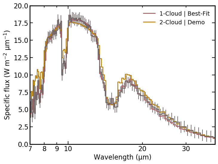
Figure 19: Comparison between the retrieved best-fit model from the single-cloud retrievals in Figure 22 (red) and a demonstration with a two-clouds model and a realistic Earth thermal structure profile (yellow).

Comparisons can be made between the MGS-TES Earth retrievals presented above and previous infrared retrieval efforts for Earth-like planets by von Paris et al. (2013) and Konrad et al. (2021), although direct comparisons are difficult as these previous studies adopted synthetic observations from cloud-free models and used constant resolving power (as a reminder, the full MGS-TES data have resolving power of 160–14 at wavelengths spanning 6–50 $\upmu$m and were trimmed to use only 7–40 $\upmu$m). The most relevant comparison point from von Paris et al. (2013) is an SNR 20 scenario with resolving power of 20 spanning 5–20 $\upmu$m. Here, surface temperature and pressure constraints are similar, but gas mixing ratio constraints are weaker in von Paris et al. (2013), likely owing to the limited number of spectral points spanning key gas absorption bands at such low resolving power. Also, constraints on the upper atmospheric temperatures are markedly weaker in results from von Paris et al. (2013), which is likely driven by a modeling approach that applies a “top of atmosphere” temperature at an atmospheric pressure of $10^{-4}$ bar where emission spectra have very little sensitivity to the thermal structure.

Work by Konrad et al. (2021) includes a relevant comparison point where the synthetic emission spectra for an Earth-like target are at a SNR of 20 and span 3–20 $\upmu$m at a resolving power of 50. Overall, constraints on gas mixing ratios, surface pressure, surface temperature, and planetary radius are comparable. As the Konrad et al. (2021) study adopted cloud-free synthetic data and models, this leads to the conclusion that thermal direct imaging missions can achieve strong constraints on key atmospheric parameters for Earth-like worlds even when the target has patchy clouds.

5.3 Cassini/VIMS Titan Discussion

Transit retrievals explored in Section 4.4 provide a strong proof-of-concept for using Solar System occultation observations as a validation point for exoplanet inference tools. While Solar System worlds with atmospheres may not be direct analogs for some exoplanet types, transit spectra and adopted error bars can be scaled to achieve a proper feature depth-to-uncertainty ratio. In general, Solar System analog transit spectra (Robinson et al., 2014; Dalba et al., 2015; Macdonald & Cowan, 2019) can be used to understand how constraints and model complexity relate to data quality and provide a timely connection to forthcoming JWST observations. The Titan retrievals presented above show gas mixing ratio constraints that are generally consistent with orbiter retrievals. Temperature constraints are biased modestly warm. As some temperature information is gleaned, in part, from a somewhat limited number of more-strongly temperature sensitive lines, the biasing may be a result of application of the HITRAN linelist at conditions far from Earth-like. Titan transit retrievals also provide an important insight into how broad gas absorption features (e.g., N₂-N₂ collision-induced absorption near 4.3 $\upmu$m) can impact haze/cloud inferences. A method for incorporating broad C-H stretch mode opacity near 3.4 $\upmu$m was presented, although such a treatment was not needed at the data qualities adopted here.

5.4 Broader Considerations

Taken altogether, the Solar System retrievals presented here show promise while also demonstrating cautionary tales. On the positive side, the wide-ranging retrieval results explored above indicate that there is great utility in using Solar System analog observations to validate and refine approaches to exoplanet remote sensing. Caution is urged, however, as many of the findings above rely on using a prior knowledge to “know” when a solution is adequate or inadequate. For example, biasing in the tropospheric thermal gradient inferred for Earth from the MGS-TES retrievals may not have been easily deduced to a truly external observer. Similarly, the addition of N₂-N₂ collision-induced absorption to the Titan-focused retrievals was introduced to better-reproduce the known wavelength-dependent slope in haze opacity.

Finally, the retrieval studies explored here — which span reflected light, thermal emission, and transit transmission — only scratch the surface of what can be learned from analog observations. Open questions remain, for example, regarding the complexity of cloud treatments warranted in reflected light retrievals, the extent to which thermal information can be extracted, and how well surface reflection signatures can be constrained. For thermal emission, an important next step is understanding how cloud treatments may (or may not) bias thermal structure inferences. Finally, Solar System transiting exoplanet analog studies provide an opportunity to test standard assumptions like constant profiles of either gas mixing ratios and/or atmospheric temperature. Any and all exoplanet-specific retrieval models could benefit from validation against Solar System observations.

6 Conclusions

Solar System observations that can serve as analogs for exoplanet observations provide unique testing and validation opportunities for exoplanet science. While such analog observations are currently limited in number, future Solar System planetary science missions could make acquisition of exoplanet analog data more standard. The utility of Solar System analog observations for exoplanets was investigated here through a broad range of scenarios, and key findings/results are:

• The new rfast retrieval suite compares well to more-sophisticated radiative transfer and inference models. This publicly-available tool was created with user-ease in mind and enables rapid and efficient explorations of how spectral data quality relates to constraints on key atmospheric and planetary parameters.

• Retrievals using the rfast model were applied to synthetic HabEx/LUVOIR-style exo-Earth observations to understand how bandpass SNR can be traded against wavelength coverage. Upper limit constraints on trace gases, such as methane and carbon dioxide — while not true detections — will still have utility for understanding exoplanet environments. The HabEx/LUVOIR-style retrievals showed that ultraviolet and/or visible data or data quality can be removed/reduced and near-infrared data qualities enhanced to achieve better constraints on difficult-to-detect gases like methane and carbon dioxide. Near-infrared SNRs of slightly greater than 45 may be required for carbon dioxide detections at the low levels present in modern Earth’s atmosphere.

• Observations of Earth from NASA’s EPOXI mission can serve as a testing ground for exo-Earth reflected light direct imaging mission concepts. Retrievals for data limited to 0.3–2.5 $\upmu$m at V-band SNR of 20 showed good constraints on gas mixing ratios and cloud parameters as well as a constraint on planet/column-averaged temperature. These are a strong proof-of-concept for a HabEx/LUVOIR-style missions, although carbon dioxide and methane constraints were enabled by features beyond 1.8 $\upmu$m. Retrievals on the same data but at a V-band SNR of 10 cannot rule out scenarios with near planet-wide cloud coverage and a deep atmosphere underneath, and distinguish this from an Earth-like atmospheric state.

• Emitted-light retrievals were performed on observations of Earth from MGS-TES instrument at a 10 $\upmu$m SNR of 20. Realistic constraints on H₂O, CO₂, O₃, N₂O, and CH₄ were achieved, which, amongst other science cases, demonstrates feasibility of detecting key biosignature gases with an infrared exo-Earth direct imaging mission. Surface pressure and planetary radius constraints were biased high and low, respectively, potentially pointing to issues with calibration and/or the treatment of water vapor pressure-induced absorption. Surface temperature was constrained to be within the habitable range, although the inferred temperature gradient in the troposphere was unrealistically small. A cloud modeling treatment that allows for multiple cloud decks was shown to potentially remedy issues with tropospheric lapse rate.

• Transit retrievals on spectra derived from Cassini-VIMS occultation observations of Titan are a strong proving ground for validation of concepts related to transiting exoplanet studies with JWST, especially as the VIMS wavelength range (0.88–5 $\upmu$m) overlaps with the ranges of several JWST instruments. At a data quality similar to previous JWST-relevant modeling studies (Greene et al., 2016), Titan transit spectra retrievals obtain gas mixing ratio constraints with uncertainties that are better than 0.5 dex and that are roughly consistent with orbiter-derived results. Constrained temperatures are biased high by about 20%, which may be due to linelist sensitivities. An approach to modeling the 3.4 $\upmu$m C-H stretch mode feature is suggested, although the VIMS-derived Titan transit spectrum can be sufficiently fitted without this treatment at the adopted noise level of 0.1 ppm.

Figure 23: Visualized posterior distribution for a 13-parameters fit to the Cassini-VIMS Titan observations (Figure 17). One-dimensional marginal distributions are shown along the diagonal with associated 16/50/84-percentile values indicated above and shown by the vertical dashed lines. Fiducial “truth” values from which the Figure 17 observed spectrum is obtained are indicated with the vertical solid lines.

References

- Akeson et al. (2019) Akeson, R., Armus, L., Bachelet, E., et al. 2019, arXiv e-prints, arXiv:1902.05569. https://arxiv.org/abs/1902.05569
- Alei et al. (2022) Alei, E., Konrad, B. S., Angerhausen, D., et al. 2022, A&A, 665, A106, doi: 10.1051/0004-6361/202243760
- Barstow et al. (2017) Barstow, J. K., Aigrain, S., Irwin, P. G. J., & Sing, D. K. 2017, ApJ, 834, 50, doi: 10.3847/1538-4357/834/1/50
- Barstow et al. (2022) Barstow, J. K., Changeat, Q., Chubb, K. L., et al. 2022, Experimental Astronomy, doi: 10.1007/s10686-021-09821-w
- Battersby et al. (2018) Battersby, C., Armus, L., Bergin, E., et al. 2018, Nature Astronomy, 2, 596, doi: 10.1038/s41550-018-0540-y
- Bean et al. (2010) Bean, J. L., Kempton, E. M.-R., & Homeier, D. 2010, Nature, 468, 669
- Bellucci et al. (2009) Bellucci, A., Sicardy, B., Drossart, P., et al. 2009, Icarus, 201, 198, doi: 10.1016/j.icarus.2008.12.024
- Benneke & Seager (2012) Benneke, B., & Seager, S. 2012, ApJ, 753, 100, doi: 10.1088/0004-637X/753/2/100
- Benneke et al. (2019) Benneke, B., Wong, I., Piaulet, C., et al. 2019, ApJ, 887, L14, doi: 10.3847/2041-8213/ab59dc
- Bétrémieux & Kaltenegger (2014) Bétrémieux, Y., & Kaltenegger, L. 2014, ApJ, 791, 7. https://arxiv.org/abs/1312.6625
- Bétrémieux & Swain (2016) Bétrémieux, Y., & Swain, M. R. 2016, ArXiv e-prints. https://arxiv.org/abs/1610.02049
- Brown et al. (2004) Brown, R., Baines, K., Bellucci, G., et al. 2004, in The Cassini-Huygens Mission (Springer), 111–168
- Buchner et al. (2014) Buchner, J., Georgakakis, A., Nandra, K., et al. 2014, A&A, 564, A125, doi: 10.1051/0004-6361/201322971
- Campargue et al. (2013) Campargue, A., Leshchishina, O., Wang, L., Mondelain, D., & Kassi, S. 2013, Journal of Molecular Spectroscopy, 291, 16, doi: 10.1016/j.jms.2013.03.001
- Christensen & Pearl (1997) Christensen, P. R., & Pearl, J. C. 1997, J. Geophys. Res., 102, 10875, doi: 10.1029/97JE00637
- Colón et al. (2020) Colón, K. D., Kreidberg, L., Welbanks, L., et al. 2020, AJ, 160, 280, doi: 10.3847/1538-3881/abc1e9
- Cours et al. (2020) Cours, T., Cordier, D., Seignovert, B., Maltagliati, L., & Biennier, L. 2020, Icarus, 339, 113571, doi: 10.1016/j.icarus.2019.113571
- Cowan et al. (2015) Cowan, N. B., Greene, T., Angerhausen, D., et al. 2015, PASP, 127, 311. https://arxiv.org/abs/1502.00004
- Dalba et al. (2015) Dalba, P. A., Muirhead, P. S., Fortney, J. J., et al. 2015, ApJ, 814, 154, doi: 10.1088/0004-637X/814/2/154
- Damiano & Hu (2021) Damiano, M., & Hu, R. 2021, AJ, 162, 200, doi: 10.3847/1538-3881/ac224d
- Dannert et al. (2022) Dannert, F., Ottiger, M., Quanz, S. P., et al. 2022, arXiv e-prints, arXiv:2203.00471. https://arxiv.org/abs/2203.00471
- Esposito et al. (2004) Esposito, L. W., Barth, C. A., Colwell, J. E., et al. 2004, Space Sci. Rev., 115, 299, doi: 10.1007/s11214-004-1455-8
- Feng et al. (2018) Feng, Y. K., Robinson, T. D., Fortney, J. J., et al. 2018, AJ, 155, 200, doi: 10.3847/1538-3881/aab95c
- Foreman-Mackey (2016) Foreman-Mackey, D. 2016, The Journal of Open Source Software, 24, doi: 10.21105/joss.00024
- Foreman-Mackey et al. (2013) Foreman-Mackey, D., Hogg, D. W., Lang, D., & Goodman, J. 2013, PASP, 125, 306, doi: 10.1086/670067
- Fortney et al. (2021) Fortney, J. J., Barstow, J. K., & Madhusudhan, N. 2021, in ExoFrontiers; Big Questions in Exoplanetary Science, ed. N. Madhusudhan (IOP Publishing, Bristol, UK), 17–1, doi: 10.1088/2514-3433/abfa8fch17
- Freedman et al. (2014) Freedman, R. S., Lustig-Yaeger, J., Fortney, J. J., et al. 2014, ApJS, 214, 25, doi: 10.1088/0067-0049/214/2/25
- Freedman et al. (2008) Freedman, R. S., Marley, M. S., & Lodders, K. 2008, ApJS, 174, 504, doi: 10.1086/521793
- Fujii et al. (2014) Fujii, Y., Kimura, J., Dohm, J., & Ohtake, M. 2014, Astrobiology, 14, 753, doi: 10.1089/ast.2014.1165
- Gaudi et al. (2018) Gaudi, B. S., Seager, S., Mennesson, B., et al. 2018, Nature Astronomy, 2, 600, doi: 10.1038/s41550-018-0549-2
- Gordon et al. (2022) Gordon, I. E., Rothman, L. S., Hargreaves, R. J., et al. 2022, J. Quant. Spec. Radiat. Transf., 277, 107949, doi: 10.1016/j.jqsrt.2021.107949
- Greene et al. (2016) Greene, T. P., Line, M. R., Montero, C., et al. 2016, ApJ, 817, 17, doi: 10.3847/0004-637X/817/1/17
- Hapke (1981) Hapke, B. 1981, J. Geophys. Res., 86, 3039, doi: 10.1029/JB086iB04p03039
- Hayne et al. (2014) Hayne, P. O., McCord, T. B., & Sotin, C. 2014, Icarus, 243, 158, doi: 10.1016/j.icarus.2014.08.045
- Heng & Li (2021) Heng, K., & Li, L. 2021, ApJ, 909, L20, doi: 10.3847/2041-8213/abe872
- Heng et al. (2021) Heng, K., Morris, B. M., & Kitzmann, D. 2021, Nature Astronomy, 5, 1001, doi: 10.1038/s41550-021-01444-7
- Henyey & Greenstein (1941) Henyey, L. G., & Greenstein, J. L. 1941, ApJ, 93, 70
- Horak (1950) Horak, H. G. 1950, ApJ, 112, 445, doi: 10.1086/145359
- Horak & Little (1965) Horak, H. G., & Little, S. J. 1965, ApJS, 11, 373, doi: 10.1086/190119
- Hubbard et al. (1993) Hubbard, W. B., Sicardy, B., Miles, R., et al. 1993, A&A, 269, 541
- Hunt (1973) Hunt, G. e. 1973, Quarterly Journal of the Royal Meteorological Society, 099, 346, doi: 10.1002/qj.49709942013
- Irwin et al. (2008) Irwin, P. G. J., Teanby, N. A., de Kok, R., et al. 2008, J. Quant. Spec. Radiat. Transf., 109, 1136, doi: 10.1016/j.jqsrt.2007.11.006
- Kaltenegger & Traub (2009) Kaltenegger, L., & Traub, W. 2009, The Astrophysical Journal, 698, 519
- Kane et al. (2019) Kane, S. R., Arney, G., Crisp, D., et al. 2019, Journal of Geophysical Research (Planets), 124, 2015, doi: 10.1029/2019JE005939
- Kane et al. (2021) Kane, S. R., Arney, G. N., Byrne, P. K., et al. 2021, Journal of Geophysical Research (Planets), 126, e06643, doi: 10.1029/2020JE006643
- Karkoschka (1998) Karkoschka, E. 1998, Icarus, 133, 134
- Kasdin et al. (2020) Kasdin, N. J., Bailey, V. P., Mennesson, B., et al. 2020, in Society of Photo-Optical Instrumentation Engineers (SPIE) Conference Series, Vol. 11443, Society of Photo-Optical Instrumentation Engineers (SPIE) Conference Series, 114431U, doi: 10.1117/12.2562997
- Keithly & Savransky (2021) Keithly, D. R., & Savransky, D. 2021, ApJ, 919, L11, doi: 10.3847/2041-8213/ac20cf
- Kitzmann et al. (2020) Kitzmann, D., Heng, K., Oreshenko, M., et al. 2020, ApJ, 890, 174, doi: 10.3847/1538-4357/ab6d71
- Knutson et al. (2014) Knutson, H. A., Dragomir, D., Kreidberg, L., et al. 2014, ApJ, 794, 155, doi: 10.1088/0004-637X/794/2/155
- Konrad et al. (2021) Konrad, B. S., Alei, E., Angerhausen, D., et al. 2021, arXiv e-prints, arXiv:2112.02054. https://arxiv.org/abs/2112.02054
- Koskinen et al. (2011) Koskinen, T. T., Yelle, R. V., Snowden, D. S., et al. 2011, Icarus, 216, 507, doi: 10.1016/j.icarus.2011.09.022
- Kreidberg et al. (2014) Kreidberg, L., Bean, J. L., Désert, J.-M., et al. 2014, Nature, 505, 69, doi: 10.1038/nature12888
- Krissansen-Totton et al. (2018) Krissansen-Totton, J., Garland, R., Irwin, P., & Catling, D. C. 2018, AJ, 156, 114, doi: 10.3847/1538-3881/aad564
- Li et al. (2018) Li, L., Jiang, X., West, R. A., et al. 2018, Nature Communications, 9, 3709, doi: 10.1038/s41467-018-06107-2
- Line et al. (2014) Line, M. R., Knutson, H., Wolf, A. S., & Yung, Y. L. 2014, ApJ, 783, 70. https://arxiv.org/abs/1309.6663
- Line et al. (2012) Line, M. R., Zhang, X., Vasisht, G., et al. 2012, ApJ, 749, 93. https://arxiv.org/abs/1111.2612
- Line et al. (2013) Line, M. R., Wolf, A. S., Zhang, X., et al. 2013, The Astrophysical Journal, 775, 137
- Livengood et al. (2011) Livengood, T. A., Deming, L. D., A’Hearn, M. F., et al. 2011, Astrobiology, 11, 907, doi: 10.1089/ast.2011.0614
- Lupu et al. (2016) Lupu, R. E., Marley, M. S., Lewis, N., et al. 2016, AJ, 152, 217, doi: 10.3847/0004-6256/152/6/217
- Lustig-Yaeger et al. (2018) Lustig-Yaeger, J., Meadows, V. S., Tovar Mendoza, G., et al. 2018, AJ, 156, 301, doi: 10.3847/1538-3881/aaed3a
- Macdonald & Cowan (2019) Macdonald, E. J. R., & Cowan, N. B. 2019, MNRAS, 489, 196, doi: 10.1093/mnras/stz2047
- MacDonald & Lewis (2021) MacDonald, R. J., & Lewis, N. K. 2021, arXiv e-prints, arXiv:2111.05862. https://arxiv.org/abs/2111.05862
- MacDonald & Madhusudhan (2017) MacDonald, R. J., & Madhusudhan, N. 2017, MNRAS, 469, 1979, doi: 10.1093/mnras/stx804
- Madhusudhan (2018) Madhusudhan, N. 2018, in Handbook of Exoplanets, ed. H. J. Deeg & J. A. Belmonte (Springer, Cham), 104, doi: 10.1007/978-3-319-55333-7_104
- Madhusudhan & Burrows (2012) Madhusudhan, N., & Burrows, A. 2012, ApJ, 747, 25, doi: 10.1088/0004-637X/747/1/25
- Madhusudhan & Seager (2009) Madhusudhan, N., & Seager, S. 2009, ApJ, 707, 24. https://arxiv.org/abs/0910.1347
- Maltagliati et al. (2015) Maltagliati, L., Bézard, B., Vinatier, S., et al. 2015, Icarus, 248, 1, doi: 10.1016/j.icarus.2014.10.004
- Mansfield et al. (2022) Mansfield, M., Wiser, L., Stevenson, K. B., et al. 2022, arXiv e-prints, arXiv:2203.01463. https://arxiv.org/abs/2203.01463
- Marley et al. (2014) Marley, M., Lupu, R., Lewis, N., et al. 2014, ArXiv e-prints. https://arxiv.org/abs/1412.8440
- Mayorga et al. (2020) Mayorga, L. C., Charbonneau, D., & Thorngren, D. P. 2020, AJ, 160, 238, doi: 10.3847/1538-3881/abb8df
- Mayorga et al. (2016) Mayorga, L. C., Jackiewicz, J., Rages, K., et al. 2016, AJ, 152, 209, doi: 10.3847/0004-6256/152/6/209
- Mayorga et al. (2021) Mayorga, L. C., Lustig-Yaeger, J., May, E. M., et al. 2021, \psj, 2, 140, doi: 10.3847/PSJ/ac0c85
- McClatchey et al. (1972) McClatchey, R. A., Fenn, R. W., Selby, J. E. A., Volz, F. E., & Garing, J. S. 1972, Optical Properties of the Atmosphere (Third Edition), Tech. rep., Air Force Cambridge Research Labs
- Meadows & Crisp (1996) Meadows, V. S., & Crisp, D. 1996, J. Geophys. Res., 101, 4595, doi: 10.1029/95JE03567
- Min et al. (2020) Min, M., Ormel, C. W., Chubb, K., Helling, C., & Kawashima, Y. 2020, A&A, 642, A28, doi: 10.1051/0004-6361/201937377
- Misra et al. (2014) Misra, A., Meadows, V., & Crisp, D. 2014, ApJ, 792, 61. https://arxiv.org/abs/1407.3265
- Mollière et al. (2019) Mollière, P., Wardenier, J. P., van Boekel, R., et al. 2019, A&A, 627, A67, doi: 10.1051/0004-6361/201935470
- Morley et al. (2016) Morley, C. V., Knutson, H., Line, M., et al. 2016, ArXiv e-prints. https://arxiv.org/abs/1610.07632
- Nayak et al. (2017) Nayak, M., Lupu, R., Marley, M. S., et al. 2017, PASP, 129, 034401, doi: 10.1088/1538-3873/129/973/034401
- Nixon & Madhusudhan (2022) Nixon, M. C., & Madhusudhan, N. 2022, arXiv e-prints, arXiv:2201.03532. https://arxiv.org/abs/2201.03532
- Pendleton & Allamandola (2002) Pendleton, Y. J., & Allamandola, L. J. 2002, ApJS, 138, 75, doi: 10.1086/322999
- Piette et al. (2022) Piette, A. A. A., Madhusudhan, N., & Mandell, A. M. 2022, MNRAS, 511, 2565, doi: 10.1093/mnras/stab3612
- Pont et al. (2008) Pont, F., Knutson, H., Gilliland, R., Moutou, C., & Charbonneau, D. 2008, Monthly Notices of the Royal Astronomical Society, 385, 109
- Porco et al. (2004) Porco, C. C., West, R. A., Squyres, S., et al. 2004, Space Sci. Rev., 115, 363, doi: 10.1007/s11214-004-1456-7
- Quanz et al. (2021a) Quanz, S. P., Absil, O., Benz, W., et al. 2021a, Experimental Astronomy, doi: 10.1007/s10686-021-09791-z
- Quanz et al. (2021b) Quanz, S. P., Ottiger, M., Fontanet, E., et al. 2021b, arXiv e-prints, arXiv:2101.07500. https://arxiv.org/abs/2101.07500
- Roberge & Moustakas (2018) Roberge, A., & Moustakas, L. A. 2018, Nature Astronomy, 2, 605, doi: 10.1038/s41550-018-0543-8
- Roberge et al. (2017) Roberge, A., Rizzo, M. J., Lincowski, A. P., et al. 2017, PASP, 129, 124401, doi: 10.1088/1538-3873/aa8fc4
- Robinson (2017) Robinson, T. D. 2017, ApJ, 836, 236, doi: 10.3847/1538-4357/aa5ea8
- Robinson & Catling (2014) Robinson, T. D., & Catling, D. C. 2014, Nature Geoscience, 7, 12, doi: 10.1038/ngeo2020
- Robinson & Crisp (2018) Robinson, T. D., & Crisp, D. 2018, J. Quant. Spec. Radiat. Transf., 211, 78, doi: 10.1016/j.jqsrt.2018.03.002
- Robinson et al. (2017) Robinson, T. D., Fortney, J. J., & Hubbard, W. B. 2017, ApJ, 850, 128, doi: 10.3847/1538-4357/aa951e
- Robinson et al. (2014) Robinson, T. D., Maltagliati, L., Marley, M. S., & Fortney, J. J. 2014, Proceedings of the National Academy of Science, 111, 9042, doi: 10.1073/pnas.1403473111
- Robinson et al. (2010) Robinson, T. D., Meadows, V. S., & Crisp, D. 2010, ApJ, 721, L67, doi: 10.1088/2041-8205/721/1/L67
- Robinson & Reinhard (2020) Robinson, T. D., & Reinhard, C. T. 2020, Earth as an Exoplanet (University of Arizona Press), 379–416. http://www.jstor.org/stable/j.ctv105bb62.21
- Robinson et al. (2011) Robinson, T. D., Meadows, V. S., Crisp, D., et al. 2011, Astrobiology, 11, 393, doi: 10.1089/ast.2011.0642
- Sidis & Sari (2010) Sidis, O., & Sari, R. 2010, The Astrophysical Journal, 720, 904
- Sing et al. (2009) Sing, D. K., Désert, J. M., Lecavelier Des Etangs, A., et al. 2009, A&A, 505, 891, doi: 10.1051/0004-6361/200912776
- Smith et al. (2020) Smith, A. J. R. W., Feng, Y. K., Fortney, J. J., et al. 2020, AJ, 159, 36, doi: 10.3847/1538-3881/ab5a8a
- Sobolev (1975) Sobolev, V. V. 1975, Light scattering in planetary atmospheres (Pergamon Press, Oxford)
- Spurr & Natraj (2011) Spurr, R., & Natraj, V. 2011, J. Quant. Spec. Radiat. Transf., 112, 2630, doi: 10.1016/j.jqsrt.2011.06.014
- Stam (2008) Stam, D. M. 2008, A&A, 482, 989, doi: 10.1051/0004-6361:20078358
- Stevenson et al. (2014) Stevenson, K. B., Désert, J.-M., Line, M. R., et al. 2014, Science, 346, 838, doi: 10.1126/science.1256758
- Swain et al. (2008) Swain, M. R., Vasisht, G., & Tinetti, G. 2008, Nature, 452, 329
- Tinetti et al. (2005) Tinetti, G., Meadows, V. S., Crisp, D., et al. 2005, Astrobiology, 5, 461
- Tinetti et al. (2006) —. 2006, Astrobiology, 6, 34, doi: 10.1089/ast.2006.6.34
- Tinetti et al. (2007) Tinetti, G., Vidal-Madjar, A., Liang, M.-C., et al. 2007, Nature, 448, 169
- Tinetti et al. (2016) Tinetti, G., Drossart, P., Eccleston, P., et al. 2016, in Society of Photo-Optical Instrumentation Engineers (SPIE) Conference Series, Vol. 9904, Space Telescopes and Instrumentation 2016: Optical, Infrared, and Millimeter Wave, ed. H. A. MacEwen, G. G. Fazio, M. Lystrup, N. Batalha, N. Siegler, & E. C. Tong, 99041X, doi: 10.1117/12.2232370
- Tomasko et al. (2008) Tomasko, M. G., Doose, L., Engel, S., et al. 2008, Planet. Space Sci., 56, 669, doi: 10.1016/j.pss.2007.11.019
- Toon et al. (1989) Toon, O. B., McKay, C., Ackerman, T., & Santhanam, K. 1989, Journal of Geophysical Research: Atmospheres (1984–2012), 94, 16287, doi: 10.1029/JD094iD13p16287
- Tremblay et al. (2020) Tremblay, L., Line, M. R., Stevenson, K., et al. 2020, AJ, 159, 117, doi: 10.3847/1538-3881/ab64dd
- Tribbett et al. (2021) Tribbett, P. D., Robinson, T. D., & Koskinen, T. T. 2021, \psj, 2, 109, doi: 10.3847/PSJ/abf92d
- Tsiaras et al. (2019) Tsiaras, A., Waldmann, I. P., Tinetti, G., Tennyson, J., & Yurchenko, S. N. 2019, Nature Astronomy, 3, 1086, doi: 10.1038/s41550-019-0878-9
- Vinatier et al. (2015) Vinatier, S., Bézard, B., Lebonnois, S., et al. 2015, Icarus, 250, 95, doi: 10.1016/j.icarus.2014.11.019
- von Paris et al. (2013) von Paris, P., Hedelt, P., Selsis, F., Schreier, F., & Trautmann, T. 2013, A&A, 551, A120, doi: 10.1051/0004-6361/201220009
- Webber et al. (2015) Webber, M. W., Lewis, N. K., Marley, M., et al. 2015, ApJ, 804, 94, doi: 10.1088/0004-637X/804/2/94
- Zhang et al. (2019) Zhang, M., Chachan, Y., Kempton, E. M. R., & Knutson, H. A. 2019, PASP, 131, 034501, doi: 10.1088/1538-3873/aaf5ad
- Zugger et al. (2010) Zugger, M. E., Kasting, J. F., Williams, D. M., Kane, T. J., & Philbrick, C. R. 2010, ApJ, 723, 1168, doi: 10.1088/0004-637X/723/2/1168